Compacti cations, Hartman functions and (weak) almost ...

GABRIEL MARESCH and REINHARD WINKLER

Compactifications, Hartman functions and(weak) almost periodicity

Gabriel MareschInstitute of Discrete Mathematics and GeometryVienna University of TechnologyWiedner Hauptstraße 8-10/1041040 Vienna, AustriaE-mail: [email protected]

Reinhard WinklerInstitute of Discrete Mathematics and GeometryVienna University of TechnologyWiedner Hauptstraße 8-10/1041040 Vienna, AustriaE-mail: [email protected]

Abstract

In this paper we investigate Hartman functions on a topological group G. Recall that (ι, C)is a group compactification of G if C is a compact group, ι : G → C is a continuous grouphomomorphism and ι(G) ⊆ C is dense. A bounded function f : G 7→ C is a Hartman functionif there exists a group compactification (ι, C) and F : C → C such that f = F ι and F isRiemann integrable, i.e. the set of discontinuities of F is a null set w.r.t. the Haar measure.In particular we determine how large a compactification for a given group G and a Hartmanfunction f : G→ C must be, to admit a Riemann integrable representation of f . The connectionto (weakly) almost periodic functions is investigated.In order to give a systematic presentation which is self-contained to a reasonable extent, weinclude several separate sections on the underlying concepts such as finitely additive measureson Boolean set algebras, means on algebras of functions, integration on compact spaces, com-pactifications of groups and semigroups, the Riemann integral on abstract spaces, invariance ofmeasures and means, continuous extensions of transformations and operations to compactifica-tions, etc.

Acknowledgements. The authors would like to thank the Austrian Science Fund (FWF) forfinancial support through grants S8312, S9612 and Y328.

2000 Mathematics Subject Classification: Primary 43A60; Secondary 26A42.Key words and phrases: Hartman function, group compactification, invariant mean, Riemann

integrable function, weakly almost periodic function

[3]

Contents

1 Introduction 5

1.1 Motivation . . . . . . . . . . . . . . . . . . . . . . . . . . . . . . . . . . . . . . . 5

1.2 Recent results on Hartman sets, sequences and functions . . . . . . . . . . . . . 7

1.3 Content of the paper . . . . . . . . . . . . . . . . . . . . . . . . . . . . . . . . . 8

2 Measure theoretic and topological preliminaries 9

2.1 Set algebras A and A-functions . . . . . . . . . . . . . . . . . . . . . . . . . . . . 9

2.2 Finitely additive measures and means . . . . . . . . . . . . . . . . . . . . . . . . 10

2.3 Integration on compact spaces . . . . . . . . . . . . . . . . . . . . . . . . . . . . 13

2.4 Compactifications and continuity . . . . . . . . . . . . . . . . . . . . . . . . . . . 15

2.5 The Stone-Cech compactification βX . . . . . . . . . . . . . . . . . . . . . . . . 19

2.6 Compactifications, measures, means and Riemann integral . . . . . . . . . . . . 20

2.7 The set of all means . . . . . . . . . . . . . . . . . . . . . . . . . . . . . . . . . . 22

3 Invariance under transformations and operations 23

3.1 Invariant means for a single transformation . . . . . . . . . . . . . . . . . . . . . 23

3.2 Applications . . . . . . . . . . . . . . . . . . . . . . . . . . . . . . . . . . . . . . 25

3.2.1 Finite X . . . . . . . . . . . . . . . . . . . . . . . . . . . . . . . . . . . . 25

3.2.2 X = Z, T : x 7→ x+ 1 . . . . . . . . . . . . . . . . . . . . . . . . . . . . . 26

3.2.3 X compact, A = C(X), T continuous . . . . . . . . . . . . . . . . . . . . 27

3.2.4 Shift spaces and symbolic dynamics . . . . . . . . . . . . . . . . . . . . . 28

3.2.5 The free group F (x, y) . . . . . . . . . . . . . . . . . . . . . . . . . . . . 29

3.3 Compactifications for transformations and actions . . . . . . . . . . . . . . . . . 29

3.4 Separate and joint continuity of operations . . . . . . . . . . . . . . . . . . . . . 31

3.5 Compactifications for operations . . . . . . . . . . . . . . . . . . . . . . . . . . . 33

3.6 Invariance on groups and semigroups . . . . . . . . . . . . . . . . . . . . . . . . 34

3.6.1 The action of a semigroup by translations . . . . . . . . . . . . . . . . . 34

3.6.2 Means . . . . . . . . . . . . . . . . . . . . . . . . . . . . . . . . . . . . . 35

3.6.3 Measures . . . . . . . . . . . . . . . . . . . . . . . . . . . . . . . . . . . . 36

3.6.4 Amenability . . . . . . . . . . . . . . . . . . . . . . . . . . . . . . . . . . 37

4 Hartman measurability 38

4.1 Definition of Hartman functions . . . . . . . . . . . . . . . . . . . . . . . . . . . 38

4.2 Definition of weak Hartman functions . . . . . . . . . . . . . . . . . . . . . . . . 40

4.3 Compactifications of LCA groups . . . . . . . . . . . . . . . . . . . . . . . . . . 42

4.4 Realizability on LCA Groups . . . . . . . . . . . . . . . . . . . . . . . . . . . . . 42

4.4.1 Preparation . . . . . . . . . . . . . . . . . . . . . . . . . . . . . . . . . . 42

4.4.2 Estimate from above . . . . . . . . . . . . . . . . . . . . . . . . . . . . . 43

4.4.3 Estimate from below . . . . . . . . . . . . . . . . . . . . . . . . . . . . . 45

[4]

5

5 Classes of Hartman functions 47

5.1 Generalized jump discontinuities . . . . . . . . . . . . . . . . . . . . . . . . . . . 47

5.2 Hartman functions that are weakly almost periodic . . . . . . . . . . . . . . . . 49

5.3 Hartman functions without generalized jumps . . . . . . . . . . . . . . . . . . . 51

5.4 Hartman functions with small support . . . . . . . . . . . . . . . . . . . . . . . . 51

5.5 Hartman functions on Z . . . . . . . . . . . . . . . . . . . . . . . . . . . . . . . . 55

5.5.1 Fourier-Stieltjes transformation . . . . . . . . . . . . . . . . . . . . . . . 56

5.5.2 Example . . . . . . . . . . . . . . . . . . . . . . . . . . . . . . . . . . . . 57

6 Summary 59

References 61

Bibliography 63

1. Introduction

1.1. Motivation. By a topological dynamical system (X,T ) we mean a continuous transforma-tion T : X → X acting on a compact space X (which in many cases is supposed to be metrizable).Symbolic dynamics is concerned with the special case X = AN or X = AZ with a finite set A,called the alphabet. Here the transformation is the shift T = σ : (an) ∈ X 7→ (an+1) ∈ X. Theimportance of this special case is due to the fact that, for a suitable finite partition (Markovpartition) X = X1 ∪ . . . ∪Xn of a metrizable space X and the alphabet A = 1, . . . , n, mostinformation of the original system (X,T ) is contained in the associated symbolic system whichis defined below.

Consider the coding F : X → A, F (x) = i if x ∈ Xi. Let ϕ : X → AN, x 7→ (Tnx)n∈N or, ifT is bijective, ϕ : X → AZ, x 7→ (Tnx)n∈Z. The case of bijective T applies for the major part ofthe exposition. The associated dynamical system (Y, σ) with Y = ϕ(X) is a subshift, i.e. Y is aclosed and σ-invariant subset of AZ. The connection between (X,T ) and (Y, σ) is expressed bythe commuting diagram:

XT - X

Y

ϕ

? σ - Y.

ϕ

?

If ϕ is continuous this means that (Y, σ) is a factor of (X,T ). However, this can be guaranteedonly if the Xi are clopen subsets of X which, for instance for connected X, is impossible. Theclassical way of avoiding this disadvantage is to choose the partition in such a way that ϕ is

6 1. Introduction

injective and ϕ−1 has a continuous extension ψ such that (X,T ) is a factor of (Y, T ):

Yσ - Y

X

ψ

? T - X.

ψ

?

In order to apply results from ergodic theory (such as Birkhoff’s Theorem) one looks for invariantmeasures. Assume that µ is such a σ-invariant measure on Y , i.e. µ(σ−1[B]) = µ(B) for all Borelsets B ⊆ Y . Then µT (M) := µ(T−1[M ]) defines a T -invariant measure µT on X.

The situation is particularly nice if T is uniquely ergodic, i.e. if there is a unique T -invariantBorel measure. In this case the limit relation

limN→∞

1

N

n−1Xn=0

f(Tnx) =

ZX

fdµT (1.1)

does hold not only up to a set of zero µT -measure, but even uniformly for all x ∈ X wheneverf : X → R is continuous and bounded. By obvious approximation this statement extends to allbounded f : X → R with

∀ε > 0 ∃f1, f2 : X → R continuous, f1 ≤ f ≤ f2,ZX

(f2 − f1)dµT < ε. (1.2)

In the case X = [0, 1], equipped with the Lebesgue measure, (1.2) is equivalent with the require-ment µT (disc) = 0, i.e. that the set disc(f) of discontinuity points of f is a null set. In otherwords, f is Riemann integrable. If f takes only finitely many values r1, . . . , rs this conditionis equivalent with µT (∂Xi) = 0 for the topological boundary of Xi := f−1[ri], i = 1, . . . , s.Indeed, this condition is usually assumed for partitions in the context of symbolic dynamics. Inthis paper we allow F : X → C to have infinitely many values, but, motivated by the aboveconsiderations, assume that F is Riemann integrable.

A very important class of uniquely ergodic systems are group rotations, i.e. T : C → C, x 7→x+g where g ∈ C is a topological generator of the compact (abelian) group C, meaning that thecyclic group generated by g is dense in C. The unique invariant measure for the transformationT is given by the Haar measure µC on C. The induced coding sequences (an)n∈Z are given byan = F (x+ ng) and may be used to form a factor of (ι, C) . Indeed, if we consider the mappingι : Z→ C, n 7→ ng, we have a = F ι. (ι, C) is a group compactification of Z since ι is a (trivial)continuous group homomorphism with image ι(Z) dense in C. Allowing Z to be replaced by anarbitrary topological group, we finally arrive at the definition of Hartman functions, the mainobjects of our paper:

A function f : G → C on a topological group G is called a Hartman function if there is agroup compactification (ι, C) of G and a function F : C → C which is Riemann integrable w.r.t.the Haar measure and satisfies f = F ι. F is called a representation of (ι, C).

In particular, almost periodic functions (defined by continuous F ) are Hartman functions.The name Hartman function refers to the Polish mathematician Stanis law Hartman who was, upto our knowledge, the first to consider these objects in the 1960s in his work in harmonic analysis[19, 20, 21]. He focused on the Bohr compactification (ιb, bG) of the group G. It is not difficult tosee that our definition is equivalent with the requirement (ι, C) = (ιb, bG). The question whetherfor a given Hartman function f , there are small compactifications with a representation f = F ιis one of our major topics.

Additionally we investigate the connection of Hartman functions and weak almost period-icity. Recall that a function is weakly almost periodic if it has a continuous representation in asemitopological semigroup compactification, or, equivalently, in the weak almost periodic com-

1.2. Recent results on Hartman sets, sequences and functions 7

pactification (ιw, wG). While every almost periodic function is Hartman, this is not true in theweak case. A more systematic overview of the content of this paper is given at the end of thisSection.

1.2. Recent results on Hartman sets, sequences and functions. For an extended surveyon recent research on Hartman sets, Hartman sequences and Hartman functions we refer to [57].Here we only give a very brief summary.

The series of papers we report on was initiated by investigations of M. Pasteka and R.F. Tichy[31, 32, 33] on the distribution of sequences induced by the algebraic structure in commutativerings R. The authors used the completion R w.r.t. a natural metric structure such that R iscompact and thus carries a Haar measure µ. The restriction of µ to the µ-continuity sets M ,i.e. to those sets with µ(∂M) = 0 has been pulled back in order to obtain a natural concept ofuniform distribution in the original structure R.

One easily observes that the measure theoretic part of the construction depends only on theadditive group structure of R. Thus the natural framework for a systematic investigation is thatof group compactifications (ι, C) of a topological group G and of the finitely additive measureµ(ι,C) on G defined for ι-preimages of µ-continuity sets as follows

µ(ι,C)

`ι−1[M ]

´:= µ(M), M ⊆ C. (1.3)

This has been studied in [12]. Results for the special case G = Z are presented in [44, 45]:Hartman sets ι−1[M ] ⊆ Z are identified with the function 1ι−1[M ] : Z → 0, 1 and calledHartman sequences. The relation to Beatty resp. Sturmian sequences and continued fractionsexpansion is described. It is shown that the system of Hartman sequences is generated by thesystem of Beatty sequences by means of Boolean combinations and approximation in measure.

The connection to ergodic theory already mentioned in [45] is stressed further in [56]: Hart-man sequences can be considered as symbolic coding sequences of group rotations (as describedin the previous section). The problem to identify the underlying dynamical system turns out tobe equivalent to the identification of the group compactification (ι, C) of Z inducing the Hartmanset ι−1[M ] ⊆ Z. As an alternative to classical methods such as spectral analysis of the dynamicalsystem, a purely topological method has been presented. Each Hartman set ι−1[M ] ⊆ Z definesin a natural way a filter on Z. Under rather mild assumptions this filter is the ι-preimage ofthe neighborhood filter U(0C) of the identity in C and contains all necessary information about(ι, C).

These methods have been applied to questions from number theory in [2] and generalized tothe setting of topological groups in [3].

The aspect of symbolic dynamics has been studied further in [47] by investigation of subwordcomplexity of Hartman sequences. Recall that the subword complexity pa : N → N induced bythe sequence a ∈ 0, 1Z is a function associating to each n ∈ N the number of different 0-1blocks of length n occurring in a. Clearly 1 ≤ pa(n) ≤ 2n. The main facts in this context are:

1. limn→∞1n

log pa(n) = 0, corresponding to the fact that group rotations have entropy 0.2. Whenever limn→∞

1n

log pn = 0 for a sequence pn with 1 ≤ pn ≤ 2n, then there is aHartman sequence a with pn(a) ≥ pn for every n ∈ N.

3. The Hartman sequence a = 1ι−1[M ], where M ⊆ Ts is an s-dimensional cube, satisfiespa(n) ∼ cM · ns with an explicit constant cM > 0 (we omit the number theoretic assump-tions).

An amazing geometric interpretation of the constant cM was recently given in [46], wherestatement 3 has been generalized to convex polygons M and cM corresponds to the volume ofthe projection body of M .

The investigation of Hartman functions has been started in [27] where, for instance, re-sults from [56] on Hartman sequences have been generalized. In the present paper we continue

8 1. Introduction

these investigations and include a systematic and considerably self-contained treatment of thetopological and measure theoretic background.

1.3. Content of the paper. Chapter 2 presents measure theoretic and topological preliminar-ies. Section 2.1 fixes notation concerning (Boolean) set algebras and related algebras of functions.In Section 2.2 we investigate finitely additive measures on set algebras and the integration offunctions from corresponding function algebras. Consequently we present the connection betweenmeasures and means. One of the most fundamental phenomena in analysis is that compactnessis used to obtain σ-additivity of measures and thus makes Lebesgue’s integration theory work.Riesz’ Representation Theorem plays a crucial role in this context, which we recall in Section2.3. For the case that compactness is absent one can try to force compactness by consideringcompactifications. In Section 2.4 we construct compactifications in such a way that a given set ofbounded functions admits continuous extensions. We touch the classical representation theoremsof Gelfand and Stone. Among all compactifications of a given (completely regular) topologicalspace X there is a, in a natural sense, maximal compactification, the Stone-Cech compacti-fication (ιβ , βX). In Section 2.5 we collect important properties. Having presented the basicsconcerning compactifications, measures, means and the Riemann integral, we put these conceptstogether in Section 2.6. Section 2.7, the last one in Chapter 2, presents the interpretation ofthe Stone-Cech compactification (ιβ , βX) of a discrete space X as the set of all multiplicativemeans on X. This motivates us to investigate means with more restrictive properties, such asinvariance.

Chapter 3 is concerned with invariance of measures and means under transformations andoperations. In particular we investigate in Section 3.1 questions of existence and uniqueness.For a transformation T : X → X invariance is closely related to the behavior of Cesaro meansalong T -orbits, a concept which leads to the notion of Banach-density. In Section 3.2 we treatseveral examples and applications: finite X, X = Z and T : x 7→ x + 1, compact X andcontinuous T : X → X, shift spaces and symbolic dynamics, the free group generated by twoelements. In Section 3.3 we consider compactifications under the additional aspect of extendingtransformations and (semi)group actions in a continuous way. For binary or, more generally,n-ary, operations continuous extensions do not always exist. The arising problems are treatedin Section 3.4. In particular n-ary operations on X, n ≥ 2, can be continuously extended to(ιβ , βX) only in very special cases. Nevertheless it is useful to formulate a general frameworkin order to unify the most interesting classical situations: topological and semitopological groupand semigroup compactifications. This is done in Section 3.5. In Section 3.6 these constructionsare discussed in the context of invariant means and measures. We mention the notion of weakalmost periodicity and touch very briefly amenable groups and semigroups.

Chapter 4 develops the basic theory of Hartman functions. Section 4.1 presents several equiv-alent conditions describing the connection with almost periodicity and the Bohr compactification,i.e. the maximal group compactification. Replacing group compactifications by semitopologicalsemigroup compactifications one obtains the weak almost periodic compactification, weak almostperiodic functions and weak Hartman functions. This is presented in Section 4.2. The categoryof all group compactifications of a topological group G is particularly well understood if G isabelian and carries a locally compact group topology. The key ingredient is Pontryagin’s DualityTheorem. We recall this situation in Section 4.3. One of the most interesting questions concern-ing a Hartman function f : G→ C is how small a group compactification (ι, C) can be taken ifone asks for a Riemann integrable representation of f . This question is treated in Section 4.4.We give an answer for LCA groups in terms of the minimal cardinality of a dense subgroup inthe Pontryagin dual G of G.

Chapter 5 is devoted to the comparison of Hartman functions and weakly almost periodicfunctions. It turns out that a generalization of what is called a jump-discontinuity in basicanalysis plays an important role. Generalized jump discontinuities are established in Section

9

5.1 and used in Section 5.2 to give necessary conditions of weak almost periodicity of Hartmanfunctions. This leads to the investigation of Hartman functions without such generalized jumpsin Section 5.3. Hartman functions with small support are treated in 5.4. Finally, Section 5.5discusses particular examples of Hartman functions on the integers which are neither almostperiodic nor converge to 0. The results use the Fourier-Stieltjes transform of measures.

Finally a short summary is given, including a diagram which illustrates the relation betweenseveral spaces of functions which are interesting in our context.

2. Measure theoretic and topological preliminaries

2.1. Set algebras A and A-functions. We start with fixing notation which is suitable toimitate the construction of the Riemann integral in the slightly more general context which willbe ours.

Definition 2.1.1. A (boolean) set algebra A (on a set X) is a system of subsets of X with∅, X ∈ A for which A,B ∈ A implies A ∪B,A ∩B,X \A ∈ A.

Example 2.1.2. Let X = [0, 1] ⊆ R be the unit interval and A = A([0, 1]) the system of all finiteunions of subintervals I ⊆ [0, 1] (open, closed and one-sided closed, also including singletons andthe empty set). This is the most classical situation. But it is worth to note that we might replace[0, 1] by any totally ordered X, for instance by any D ⊆ [0, 1] dense in [0, 1] (as D = Q ∩ [0, 1]).

We are interested in the integration of complex valued functions on X:

Definition 2.1.3. Let A be a set of functions f : X → C. We call the subset AR of all f ∈ Awith f(X) ⊆ R the real part of A. A is called real if AR = A. If A is a vector space or analgebra over R (or C) we call A a real (or complex) space resp. a real (or complex) algebra offunctions. For any A ⊆ X let 1A(x) = 1 for x ∈ A and 1A(x) = 0 for x ∈ X \A. For an algebraA we always assume 1X ∈ A. A complex space or algebra A of functions is called a ∗-spaceresp. a ∗-algebra if f ∈ A implies f ∈ A for the complex conjugate f of the function f . Wewrite B(X) for the set of all bounded f : X → C, BR(X) := B(X)R for its real part. (Laterwe will also use the notation B for the Fourier-Stieltjes algebra.) A *-algebra A on X which iscomplete with respect to the topology of uniform convergence on X is called a C∗-algebra.

Note that whenever A is a real space we can form the complexification AC = f1 + if2 :f1, f2 ∈ A which is a complex vector space, and a ∗-algebra whenever A is a real algebra.For any complex linear space or algebra A, to be a ∗-space resp. a ∗-algebra is equivalent withthe following property: Whenever f = f1 + if2 is the decomposition of f into real part f1 andimaginary part f2, then f ∈ A if and only if f1, f2 ∈ AR. Thus for the investigation of ∗-algebrasA it suffices to investigate the real part AR whenever convenient. Furthermore any ∗-algebra

of functions is closed under taking absolute values: |f | =pff ; a fact which can be seen by

approximating the square-root by polynomials.

Definition 2.1.4. Let A be a set algebra on X. A function f : X → C is called A-simple if ithas a representation

f =

nXi=1

ci1Ai

with Ai ∈ A and ci ∈ C. The set of all A-simple f is denoted by SA. We denote the uniformclosure SA of SA by B(A). Members of B(A) are also called A-functions.

More explicitly, for a set algebra A on X the function f : X → C lies in B(A) if and only iffor all ε > 0 there is a f ′ ∈ SA with |f(x)− f ′(x)| < ε for all x ∈ X.

10 2. Measure theoretic and topological preliminaries

Proposition 2.1.5. All of the sets SA ⊆ B(A) ⊆ B(X) are ∗-algebras. In general the inclusionscannot be replaced by equality.

Proof. It is clear that SA, B(A) and B(X) are ∗-algebras satisfying the stated inclusions. Thusit suffices to show that SA 6= B(A) 6= B(X) if one takes X = [0, 1] and A = A([0, 1]), the setalgebra of all finite unions of subintervals of [0, 1]. Then f ∈ C(X) ⊆ B(A) but f /∈ SA if wetake f(x) = x, hence SA 6= B(A). On the other side all f ∈ B(A) are Riemann integrable in theclassical sense which is not the case for arbitrary f ∈ B(X).

For every set algebra A, B(A) is a C∗-algebra. But not every C∗-algebra A can be writtenas A = B(A) for an appropriate A. The situation is explained by the following facts.

Proposition 2.1.6. For a set A of complex valued functions f : X → C let AA := A ⊆ X :1A ∈ A. Then:

1. AA is a set algebra whenever A is an algebra.2. Every set algebra A on X satisfies A = AB(A).3. For every uniformly closed algebra A one has B(AA) ⊆ A while the converse inclusion

does not hold in general.

Proof.1. Follows from 1X ∈ A, 1A1∩A2 = 1A1 · 1A2 , 1X\A = 1X − 1A and the identity A1 ∪A2 =

X \ ((X\A1) ∩ (X\A2)).2. The inclusion A ⊆ AB(A) is obvious. For the converse assume A ∈ AB(A), i.e. 1A ∈ B(A).

Then there are fn ∈ SA uniformly converging to 1A. There are representations fn =Pkni=1 αi,n1An,i such that for each n the An,i ∈ A, i = 1, . . . , kn, are pairwise disjoint.

For sufficiently large fixed n, each x ∈ X satisfies either |fn(x) − 1| < 12

(if x ∈ A) or|fn(x)| < 1

2(if x /∈ A). This shows that An,i ⊆ A or An,i ⊆ X \ A for any such fixed n

and all i = 1, . . . , kn, hence A =Si:An,i⊆AAn,i ∈ A.

3. The stated inclusion is obvious. The example A = C([0, 1]), AA = ∅, X, B(AA) =c1X : c ∈ C, shows that the inclusion might be strict.

2.2. Finitely additive measures and means.

Definition 2.2.1. Let A be a set algebra on X. A function p : A → [0,∞] with p(∅) = 0 iscalled a finitely additive measure, briefly fam (on X or, more precisely, on A) if it is finitelyadditive, i.e. if p(A1∪A2) = p(A1)+p(A2) whenever A1∩A2 = ∅. p is called a finitely additiveprobability measure, briefly fapm, if furthermore p(X) = 1.

Example 2.2.2. Continuing Example 2.1.2, for X = [0, 1] and A = A([0, 1]), the system of allfinite unions of intervals, one takes p(I) = b− a for I = [a, b] with 0 ≤ a ≤ b ≤ 1. This definitionuniquely extends to a fapm on the set algebra A([0, 1]) of all finite unions of intervals. We willrefer to this p as the natural measure. The construction does not depend on the completeness(compactness) of [0, 1] and hence can be done as well for dense subsets D ⊂ X. For instance onecould consider (finite unions of) intervals of rationals.

Definition 2.2.3. Let A be a linear space of functions on a set X. Then a mean m on A isa linear functional m : A → C which is positive, i.e. f ≥ 0 implies m(f) ≥ 0, and satisfiesm(1X) = 1.

Note that whenever A is real and m is a mean on A then m(f1 + if2) := m(f1) + im(f2)for f1, f2 ∈ A is the unique extension m to the complexification AC of A. Very often we simplywrite m for m.

For real functions f every mean m, by positivity, satisfies inf f ≤ m(f) ≤ sup f . As aconsequence we have:

2.2. Finitely additive measures and means 11

Proposition 2.2.4. Every mean m on A is continuous with respect to the norm ||f ||∞ :=supx∈X |f(x)| and thus has a unique extension to the uniform closure A of A.

Every mean induces a further notion of closure:

Definition 2.2.5. Let m be a mean on a linear space A of functions on X. Then the real m-

closure AR(m)

of A is the set of all f : X → R such that for all ε > 0 there are f1, f2 ∈ AR with

f1 ≤ f ≤ f2 and m(f2 − f1) < ε. For f ∈ AR(m)

, m(f) is defined to be the unique value α ∈ Rwith m(f1) ≤ α ≤ m(f2) for all f1, f2 ∈ A with f1 ≤ f ≤ f2. The (complex) m-closure A(m)

is

the set of all f = f1 + if2 with f1, f2 ∈ A(m)R . Furthermore we define m(f) := m(f1) + im(f2)

for such f = f1 + if2. m is called the completion of m, sometimes also simply denoted by m.

In the case A(m)= A we call m complete and A m-closed.

Remark 2.2.6. Distinguish the m-closure from the completion with respect to the pseudo-metricdm(f, g) := m(|f−g|). By definition (m is continuous w.r.t. dm) them-closure is always contained

in the dm-completion: A(m) ⊆ A(dm). The closure w.r.t. m corresponds to the integral in the

sense of Riemann, the completion w.r.t. dm to that of Lebesgue (modulo null-sets).

Every fapm p defined on a set algebra A on a set X induces a linear functional mp in thenatural way. Standard arguments (using that A is closed under intersections and that p is finitelyadditive) show that for an A-simple f =

Pni=1 ci1Ai ∈ SA the value

mp(f) = mp

nXi=1

ci1Ai

!:=

nXi=1

cip(Ai)

does not depend on this particular representation of f as a linear combination. Obviously thismp is a mean on SA and thus, by Proposition 2.2.4, has a unique extension to the algebra

B(A) = SA as well as to SA(mp)

.We want to extend the domain of mp from SA to the space Ip defined as follows.

Definition 2.2.7. For a given fapm p on A let Ip := S(mp)

A . The members f ∈ Ip are calledintegrable (w.r.t. p). The extension of mp to Ip, usually also denoted by mp, is called the meaninduced by p.

We leave the proof of the following easy properties to the reader:

Proposition 2.2.8. Let A be a set algebra on the set X, p a fapm defined on A. Then B(A) ⊆Ip ⊆ B(X), Ip is mp-closed and mp is a mean on Ip.

Remark 2.2.9. Ip is uniformly closed. In particular Ip is a C∗-algebra. Indeed, let fn → funiformly where fn ∈ Ip. For given ε > 0 there exists fn such that ‖f − fn‖∞ ≤ ε

4and

fn,1, fn,2 ∈ B(A) such that fn,1 ≤ fn ≤ fn,2 and mp(fn,2 − fn,1) ≤ ε2. Observe that

fn,1 − ε4≤ fn − ε

4≤ f ≤ fn + ε

4≤ fn,2 + ε

4

and thus mp

`(fn,2 + ε

4)− (fn,1 − ε

4)´≤ ε shows f ∈ Ip.

The inclusions stated in Proposition 2.2.8 are in general strict as the following exampleshows.

Example 2.2.10. Let again A = A([0, 1]) be the set algebra of all finite unions of subintervalsof X = [0, 1], p the natural measure on A. Then Ip is the set of all f : [0, 1] → C which areintegrable in the classical Riemann sense, thus a proper subset of B(X). Consider f := 1C

where C =˘P∞

n=1an3n

: an ∈ 0, 2¯

is Cantor’s middle third set. Then f ∈ Ip, but f /∈ B(A):

f ∈ B(A) would yield the existence of f1 =Pni=1 ci1Ai ∈ SA with Ai ∈ A, ci ∈ C and

||f−f1||∞ < 12. We may assume that the Ai are pairwise disjoint. Consider A :=

Si:|ci−1|< 1

2Ai ∈

A and f2 := 1A ∈ SA. Then ||f − f2||∞ < 12

which, since f and f2 only take the values 0 and 1,implies f = f2 and C = A, a finite union of intervals, contradiction.


We have seen that each fapm p on a set algebra in a natural way induces a mean m on the C∗-algebra Ip. Recall from the first statement in Proposition 2.1.6 that AA := A ⊂ X : 1A ∈ Ais a set algebra whenever A is an algebra of functions. Given a mean m on A, pm(A) := m(1A)clearly defines a fapm on Am := AA. We ask whether the constructions ϕ : (A, p) 7→ (Ip,mp)and ψ : (A,m) 7→ (Am, pm) are inverse to each other. In general this is not the case.

Example 2.2.11. Consider any algebra A of continuous functions on a nontrivial connected spaceX (for instance X = [0, 1]) containing functions which are not constant, and any nontrivial meanm on A. Then AA = ∅, X and hence Ipm only contains the constant functions and does notcoincide with A.

However, this is not surprising if we note that A in the above example is not m-closed, whileIp is mp-closed. Thus we have to assume this property for all function algebras and means, andto use the analogue property for fapm’s.

Definition 2.2.12. Consider a fapm p on a set algebra A on the set X. Then the p-completion

A(p)

of A is defined as the set of all A ⊆ X with the following property: For each ε > 0 there are

A1, A2 ∈ A with A1 ⊆ A ⊆ A2 and p(A2 \A1) < ε. For A ∈ A(p)

we define p(A) to be the uniqueα with p(A1) ≤ α ≤ p(A2) for all A1, A2 ∈ A with A1 ⊆ A ⊆ A2. In this way we canonically

extend p to all of A(p)

. In the case A(p)

= A we call p complete and A p-closed.

It is clear that the p-completion of a set algebra is again a set algebra. Note furthermorethat in the case that p is σ-additive the notion coincides with the usual concept of a completemeasure.

Proposition 2.2.13. Let A be a set algebra on X and p a fapm on A.

1. A ⊆ Amp and pmp(A) = p(A) whenever A ∈ A.

2. A(p)

= Amp . In particular the equality A = Amp holds if and only if A is p-closed.

Proof. The first statement is obvious. To prove the second statement assume first that A ∈ Ampand pick any ε > 0. Then we have, by definition of Amp , that 1A ∈ Ip. By definition of Ipthis means that there are f1, f2 ∈ SA such that f1 ≤ 1A ≤ f2 and mp(f2 − f1) < ε. There is arepresentation f2 − f1 =

Pni=1 ci1Ai such that the Ai are nonempty, pairwise disjoint and both

f1 and f2 are constant on each Ai. f2 − f1 ≥ 0 implies ci ≥ 0 for all i. Consider the partitionof 1, . . . , n into three sets I1, I2, I3 in such a way that Ai ⊆ A for i ∈ I1 and Ai ∩ A = ∅ fori ∈ I2. For i ∈ I3 we require that Ai intersects A as well as X \ A. We define B1 :=

Si∈I1 Ai

and B2 := B1 ∪Si∈I3 Ai, hence B1 ⊆ A ⊆ B2 and B1, B2 ∈ A. Note that f1 ≤ 1A ≤ f2 together

with the fact that the f1 and f2 are constant on each Ai implies that for i ∈ I3 we have f1 ≤ 0and f2 ≥ 1, therefore ci ≥ 1. We conclude

p(B2 \B1) =Xi∈I3

p(Ai) ≤Xi∈I3

cip(Ai) = mp

Xi∈I3

ci1Ai

!

≤ mp

nXi=1

ci1Ai

!= mp(f2 − f1) < ε.

Since ε > 0 was arbitrary this implies A ∈ A(p)

.

If on the other hand we are given a set A ∈ A(p)

and ε > 0, then there exist B1, B2 ∈ A suchthat B1 ⊆ A ⊆ B2 and p(B2 \B1) < ε. Passing to the indicator functions 1B1 ≤ 1A ≤ 1B2 andnoting 1B1 ,1B2 ∈ SA we see that A ∈ Amp .

The analogue statement for the converse construction says that, given a mean m on a C∗-algebra A, A = Ipm if and only if A is m-closed. Later we will use topological constructions fora proof of this fact, see Proposition 2.6.6.

2.3. Integration on compact spaces 13

2.3. Integration on compact spaces. Throughout this text the notion of compactness alwaysincludes the Hausdorff separation axiom. In this section we assume that X is a compact space.If µ is a Borel probability measure on X then m = mµ : f 7→

RXfdµ defines a mean on

A = C(X), the C∗-algebra of all continuous f : X → C. One of the main reasons that integrationtheory is particularly successful on (locally) compact spaces is that also a converse is true:Positive functionals induce σ-additive measures. This is the content of the celebrated Riesz’Representation Theorem, which we use in the following version:

Proposition 2.3.1 (Riesz). Let X be compact and m a mean on C(X). Then there is a uniqueregular probability measure µ = µm which is the completion of its restriction to the σ-algebra ofBorel sets on X and such that m(f) =

RXfdµ for all f ∈ C(X). (Recall that regular means

that for every µ-measurable A and all ε > 0 there are closed F and open G with F ⊆ A ⊆ G andµ(G \ F ) < ε.)

A proof can be found for instance in Rudin’s book [38].

On the compact unit interval X = [0, 1] the classical Riemann integral can be taken as amean m on C(X). Then the measure µm according to Riesz’ Representation Theorem is theLebesgue measure on [0, 1]. Note that in this case A = C(X) is not mµ-closed, since all Riemannintegrable functions (essentially by the very definition of the Riemann integral) are membersof the m-closure of A but not necessarily continuous. Sets A with topological boundary ∂A ofmeasure 0 play an important role.

Definition 2.3.2. Let µ be a complete Borel measure on X. A set A ⊆ X is called µ-Jordanmeasurable or a µ-continuity set if the topological boundary ∂A of A satisfies µ(∂A) = 0.The system of all µ-continuity sets (which forms a set algebra on X) is denoted by Cµ(X).

In the classical case X = [0, 1], µ the Lebesgue measure, the continuity sets A are exactlythose A ⊆ [0, 1] for which 1A is integrable in the Riemann sense. The uniform closure of thelinear span of such 1A coincides with the Riemann integrable functions. In order to treat theRiemann integral in the context of compactifications we fix well-known characterizations ofclassical Riemann integrability in our somewhat more general context.

For a function f , defined on the topological space X, we will denote by disc(f) the set ofdiscontinuity points of f .

Proposition 2.3.3. Let X be compact, µ a finite complete regular Borel measure on X andf : X → R bounded. Then the following conditions are equivalent:

1. disc(f) is µ-measurable and a µ-null set.

2. f ∈ SCµ = B(Cµ), i.e. f can be approximated by simple Cµ-functions w.r.t uniform con-vergence.

3. f ∈ C(X)mµ

, i.e. for every ε > 0 there exist f1, f2 ∈ C(X) such that f1 ≤ f ≤ f2 andRX

(f2 − f1)dµ < ε.

If one (and hence all) of these conditions are satisfied, then f is µ-measurable.

Proof. First we prove that condition 1. implies that f is measurable. By regularity there is adecreasing sequence of open sets On, n ∈ N, of measure µ(On) < 1

nwith disc(f) ⊆ On. Let fn

be the restriction of f to X \On. For any Borel set B ⊆ R we have f−1[B] =Sn∈N f

−1n [B] ∪N

with N ⊆ D :=Tn∈N On, µ(D) = 0. By the completeness of µ we conclude that N and thus

f−1[B] and finally f is measurable. Now we start with the cyclic proof of the equivalences.

1 ⇒ 2: Assume that µ(disc(f)) = 0 and, w.l.o.g. that f(X) ⊆ [0, 1]. We introduce thelevel-sets Mt := [0 ≤ f < t] which are measurable by the first part of the proof, and the function

ϕf (t) := µ(Mt).


Since ϕf is increasing, it has at most countably many points of discontinuity. Consider µ(x :f(x) = t) ≤ ϕf (r)− ϕf (s) for s < t < r. If ϕf is continuous at t this implies

sups<t

ϕf (s) = f(t) = infr>t

ϕf (r),

and so x : f(x) = t is a µ−null set for t /∈ disc(ϕf ). Now let x ∈ ∂Mt. If f is continuous at xwe clearly have f(x) = t. So

∂Mt ⊆ disc(f) ∪ x : f(x) = t.

The first set on the right-hand side is a µ−null set by our assumption and the second one is aµ-null set at least for each continuity point t of ϕf . So for all but at most countably many t theset Mt is a µ-continuity set. In particular the set Nf := t : µ(∂Mt) = 0 ⊆ [0, 1] is dense.

Now we approximate f uniformly by members of SCµ : Given ε > 0, pick n ∈ N such thatn > 1

εand pick real numbers tini=0 ⊂ Nf with

t0 = 0 < t1 <1

n< . . . < ti <

i

n< ti+1 < . . . <

n− 1

n< tn = ‖f‖∞ ≤ 1.

Let Ai := Mti\Mti−1 . Then |f(x)− i−1n| < ε on Ai, i = 1, . . . , n. Since X = M1 \M0 =

Sni=1Ai

we conclude ˛ nXi=1

i

n1Ai(x)− f(x)

˛< ε.

2⇒ 3: Let A0 denote the set of all bounded g : X → R satisfying Condition 3, i.e. such thatfor each ε > 0 there are g1, g2 ∈ C(X) with g1 ≤ g ≤ g2 and

RX

(g2 − g1) dµ < ε. It is a routinecheck that A0 is a linear space and uniformly closed. Thus it suffices to show that 1A ∈ A0

whenever A ∈ Cµ. For such an A and any given ε > 0 we use the regularity of µ to get an openset O with ∂A ⊆ O and µ(O) < ε. Since compact spaces are normal we can find closed setsA1, A2 and open sets O1, O2 with

A \O ⊆ O1 ⊆ A1 ⊆ Ao ⊆ A ⊆ O2 ⊆ A2 ⊆ A ∪O.

Take continuous Urysohn functions f1 for A \O and X \O1, f2 for A2 and X \ (A ∪O), i.e.

1A\O ≤ f1 ≤ f ≤ f2 ≤ 1A∪O.

ThenRX

(f2 − f1) dµ ≤ µ(O) < ε.

3⇒ 1: Define the oscillation Osf (x) of f at a point x by

Osf (x) := lim supy→x

f(y)− lim infy→x

f(y).

Let Ak := [Osf (x) ≥ 1k

] be the set of all x ∈ X where the oscillation of f is at least 1k

. Pickany ε > 0 and k ∈ N. By Condition 3 there are continuous fε1 , f

ε2 with fε1 ≤ f ≤ fε2 andR

X(fε2 − fε1 ) dµ < ε

k. Note that Ak ⊆ Bεk := x ∈ X : fε2 (x)− fε1 (x) ≥ 1

k and µ(Bεk) < 2ε. Since

ε > 0 was arbitrary we have µ(Ak) = 0. Since disc(f) =Sk∈N Ak this proves Condition 1.

The equivalence of 1 and 3 can also be found in [49].

Definition 2.3.4. Let µ be a finite, complete and regular Borel measure on the compact spaceX and f : X → C be a bounded function with decomposition f = f1+if2 into real and imaginarypart. Then f is called µ-Riemann integrable if both f1 and f2 satisfy the equivalent conditionsof Proposition 2.3.3. We denote the set of all µ-Riemann integrable f by Rµ(X) or Rµ.

The three conditions in Proposition 2.3.3 immediately transfer to complex valued functions.

Corollary 2.3.5. Let µ be a finite, complete and regular Borel measure on the compact spaceX. For a bounded f : X → C the following conditions are equivalent.

1. f ∈ Rµ, i.e. f is µ-Riemann integrable.

2.4. Compactifications and continuity 15

2. µ(disc(f)) = 0.3. f ∈ B(SCµ).

In particular Rµ = Ip if p(A) := µ(A) for A ∈ Cµ.

Every f ∈ Rµ is µ-measurable and the set disc(f) of discontinuities of a Riemann integrablef is small not only in the measure theoretic but also in the topological sense.

Proposition 2.3.6. Let X be compact and µ a finite regular Borel measure, supp(µ) = X .Letf ∈ Rµ(X) be Riemann integrable. Then disc(f) is a meager µ-null set, in particular the set ofcontinuity points of f is dense in X.

Proof. We may assume that f ∈ Rµ(X) is real-valued. It suffices to show that disc(f) is meager.As in the proof of Proposition 2.3.3 let us denote the oscillation of f at x by Osf (x). A standardargument shows that the sets An := [Osf ≥ 1

n], n > 0 are closed. The sets An are all µ-null

sets since An ⊆ disc(f). Using that µ has full support, this implies that all sets An are nowheredense, i.e. disc(f) =

Sn>0An is a meager Fσ-set of zero µ−measure.

We want to illustrate the role of the regularity assumption on µ in Proposition 2.3.3. Forthis we use the example of a non regular Borel measure occurring in Rudin’s book [38, Exercise2.18].

Example 2.3.7. Let X = [0, ω1] be the set of all ordinals up to the first uncountable one equippedwith the order topology. Thus X is a compact space.

We need the fact that every (at most) countable family of uncountable compact subsetsKn ⊆ X has an uncountable intersection K. To see this consider any increasing sequence x0 <x1 < x2 < . . . ∈ X which meets every Kn infinitely many times. It follows that α0 := supn xn <ω1 is in the closure of all Kn, hence in K. Since we may require x0 > x for any given x < ω1

the same construction can be repeated in order to obtain an α1 ∈ K with α1 > α0. Transfiniteinduction with the limit step αλ := supν<λ αν generates the closed and thus compact subset ofall αν , ν < ω1, which is contained in K.

Easy consequences: We call a set S ⊆ X of type 1 if S ∪ ω1 contains an uncountablecompact K. If S is of type 1 the complement of S must not have the same property. Call S ⊆ Xof type 0 if (X \ S)∪ ω1 contains an uncountable compact K. The system of all sets of eithertype 0 or type 1, forms a σ-algebra A containing all Borel sets.

Letting µ(S) = i if S is of Type i = 0, 1, µ is a complete measure defined on A. Note thatevery countable set is a µ-null set. The set ω1 has measure 0 and is a counterexample forouter regularity: The function 1ω1 obviously satisfies conditions 1 and 2 in Proposition 2.3.3,but not condition 3. To see this last assertion consider any continuous f : X → C and take βnsuch that |f(x) − f(ω1)| < 1

nfor all x ≥ βn. Then β := supn βn < ω1 has the property that

f(x) = f(ω1) for all x ≥ β. It follows thatRXf dµ = f(ω1) for all f ∈ C(X). In particular

g ≤ 1ω1 ≤ h, g, h ∈ C(X) impliesRX

(h− g) dµ ≥ 1, contradicting condition 3.Nevertheless we might apply Riesz’ Representation Theorem 2.3.1 to the functional m(f) :=R

Xf dµ. A quick inspection shows that µm = δω1 , i.e. the associated unique regular Borel

measure is the point measure concentrated at the point ω1. As a complete measure, this µm isdefined on the whole power set of X. Finally we observe that 1ω1 /∈ Iµm .

2.4. Compactifications and continuity. The previous Section has illustrated that compact-ness plays an important role in integration theory. This motivates us to investigate compactifi-cations, the topic of this purely topological Section. Let X be a, possible discrete, topologicalspace.

We will interpret functions f : X → C as restrictions of functions F : K → C on compactspaces K. For our needs the following setting is appropriate.

Definition 2.4.1. A pair (ι,K), K compact, ι : X → K a continuous mapping, is called acompactification of X whenever ι(X) = K, i.e. whenever the image of X under ι is dense in


K. The function F : K → C is called a representation of f : X → C whenever f = F ι, i.e.whenever the diagram

K

Xf -

ι

-

C

F

?

commutes. In this case we also say that f can be represented in (ι,K). If F ∈ C(K) we say thatF is a continuous representation.

Note that in the definition of a compactification ι is neither required to be a homeomorphicembedding nor to be injective. If there is a continuous representation F of f in (ι,K), thenthis F is uniquely determined by continuity and the fact that ι(X) is dense in K. Furthermoref = F ι is continuous as well. In this Section we are therefore mainly interested in continuousf . Let us consider first a rather trivial example.

Example 2.4.2.

• Let f : X → C be bounded and continuous. Surely Kf := f(X) is compact. Defineιf : x 7→ f(x) and let Ff : Kf → C be the inclusion mapping. Then (ιf ,Kf ) is acompactification of X and Ff is a continuous representation of f in (ιf ,Kf ). We call Ffthe natural continuous representation of f .

• Let f : X → C be merely bounded. If we impose the discrete topology on X, f iscontinuous and the associated compactification (ιf ,Kf ) is then a compactification of thediscrete space Xdis.

One observes the following minimality property of the natural continuous representation:If F : K → C is any continuous representation of f in any compactification (K, ι) of X, thenπ : K → Kf = f(X), π(k) := F (k), is continuous, onto and satisfies π ι = ιf . This motivatesthe following definition.

Definition 2.4.3. Let (ι1,K1) and (ι2,K2) be two compactifications of X. Then we write(ι1,K1) ≤ (ι2,K2) (via π) and say that (ι1,K1) is smaller than (ι2,K2) or, equivalently, (ι2,K2)is bigger than (ι1,K1), if π : K2 → K1 is continuous satisfying ι1 = π ι2, i.e. making thediagram

K2

Xι1 -

ι2

-

K1

π

?

commutative. For the case that π is a homeomorphism we say that (ι1,K1) and (ι2,K2) areequivalent via π and write (ι1,K1) ∼= (ι2,K2).

A consequence of the continuity of the involved maps and of the fact that the images ιi(X)are dense is that π as in Definition 2.4.3 is unique. By compactness, π is onto as well. If π happensto be injective it is a homeomorphism, i.e. (ι1,K1) and (ι2,K2) are equivalent. Furthermore oneeasily sees that, whenever (ι1,K1) ≤ (ι2,K2) via π1 and (ι2,K2) ≤ (ι1,K1) via π2 then π2 π1 isthe identity on K1 and π1π2 is the identity on K2, hence π2 = π−1

1 , π1 and π2 are isomorphismsand both compactifications are equivalent.

Proposition 2.4.4. (ι1,K1) ∼= (ι2,K2) if and only if both, (ι1,K1) ≤ (ι2,K2) and (ι2,K2) ≤(ι1,K1).

2.4. Compactifications and continuity 17

Note that maps π1, π2 as in Definition 2.4.3 may as well be considered to be the morphismsin a category whose objects are all compactifications of X. Other related categories arise if oneallows only continuous representations of one fixed f : X → C. In this terms the minimalityproperty of the natural compactification asserts that (ιf ,Kf ) is a universal object and thusunique up to equivalence.

Proposition 2.4.5. Let F1 be a representation of f : X → C in a compactification (ι1,K1) ofX, and suppose (ι1,K1) ≤ (ι2,K2) via π. Then F2 := F1 π is a representation of f in (ι2,K2)which is continuous whenever F1 is continuous.

Given a family of compactifications (ιi,Ki), i ∈ I, of X, we get a common upper bound bytaking products: Let ι(x) := (ιi(x))i∈I ∈ P :=

Qi∈I Ki and K := ι(X) ⊆ P . Then one obtains

a compactification (ι,K) which, by the projections πi0 : K → Ki0 , i0 ∈ I, (ki)i∈I 7→ ki0 , indeedsatisfies (ιi,Ki) ≤ (ι,K) for all i ∈ I. Sometimes we use the notation

Wi∈I(ιi,Ki) for (ι,K).

Definition 2.4.6. For compactifications (ιi,Ki) of X, i ∈ I, the compactification (ι,K), ι : x 7→(ιi(x))i∈I , K := ι(X) ⊆

Qi∈I Ki, is called the product compactification of all (ιi,Ki), i ∈ I.

Proposition 2.4.7. For compactifications (ιi,Ki) of X, i ∈ I, the supremum supi∈I(ιi,Ki) isequivalent to the product compactification (ι,K) of all (ιi,Ki), i ∈ I.

Proof. We have already seen that supi∈I(ιi,Ki) ≤ (ι,K). Let (ι′,K′) be another compactifica-tion of X such that (ιi,Ki) ≤ (ι′,K′), i ∈ I. Denote by πi : K′ → Ki the i-th projection. Definea mapping π : K′ → K via k′ 7→ (πi(k

′))i∈I . Note that π ι′ = ι, hence π(ι′(X)) ⊆ K and

π(K′) = π(ι′(X)) ⊆ π(ι′(X)) ⊆ K.

It is immediate to check that π is continuous; thus (ι,K) ≤ (ι′,K′).

Analogously the product compactification can be used to obtain a minimal compactificationwhere all functions from an arbitrary given family have a continuous representation: Let fi :X → C, i ∈ I, be bounded and continuous functions on X. We consider the natural continuousrepresentations of the fi, i.e. (ιi,Ki) := (ιfi ,Kfi) and Fi : Ki → C, the inclusion mappings. Let(ι,K) be the product of all (ιi,Ki), i ∈ I.

Definition 2.4.8. Let us denote the C∗-algebras of bounded resp. continuous resp. boundedand continuous f : X → C by B(X), C(X) resp. Cb(X). For a given family of fi ∈ Cb(X), i ∈ I,the compactification (ι,K), constructed as above is called the natural compactification forthe family of all fi, i ∈ I. If A = fi : i ∈ I we also write (ιA,KA) for (ι,K).

Proposition 2.4.9. Let A ⊆ Cb(X), then the following holds

1. Every f ∈ A has a continuous representation in the natural compactification (ιA,KA) ofA.

2. Suppose that (ι,K) is any compactification of X where every f ∈ A has a continuous rep-resentation. Then (ιA,KA) ≤ (ι,K), i.e. (ιA,KA) is minimal among the compactificationswith this property .

3. F ι : F ∈ C(KA) is a C∗-algebra and the ∗-algebra generated by A is dense in thisC∗-algebra. In particular, if A is C∗-algebra, then A contains exactly those f which havea continuous representation in (ιA,KA).

Proof.

1. For each i0 ∈ I, Gi0 : K → C, (ci)i∈I 7→ ci0 , is continuous and satisfies fi0 = Gi0 ι foreach i0 ∈ I. Thus all fi can be continuously represented in (ιA,KA).

2. Let (ι′,K′) be an arbitrary compactification of X where continuous representations G′i :K′ → C of fi = G′i ι′ exist. As in Proposition 2.4.7 we define π : k′ 7→ (G′i(k

′))i∈I ∈Qi∈I fi(X). π is continuous because all components are. Again we have π(K′) ⊆ K,


π : K′ → K and (ι,K) ≤ (ι′,K′). Furthermore G′i = Gi π for all i ∈ I, since themappings on both sides are continuous and coincide on the dense set ι′(X).

3. It is clear that the mapping F 7→ F ι maps the C∗-algebra C(KA) again on a C∗-algebraand that this map is a continuous homomorphism between C∗-algebras.For the rest of the proof we can assume w.l.o.g. that A is a ∗-algebra. It remains to provethat the ∗-algebra A′ := F ∈ C(KA) : F ι ∈ A is dense in C(KA). We employ theStone-Weierstraß theorem. Obviously A′ is a ∗-algebra containing all constant functions.We are done if A′ is point separating. Pick c 6= c′ ∈ KA. Recall that the points in KAare of the form c = (cf )f∈A and c′ = (c′f )f∈A with cf , c

′f ∈ C. Hence there is some

f0 ∈ A such that cf0 6= c′f0 . By definition, KA is the closure of the set of all (f(x))f∈A,x ∈ X. It follows that there are x, x′ ∈ X with f0(x) arbitrary close to cf0 , f0(x′) toc′f0 , hence f0(x) 6= f0(x′). Let F0 = πf0 ∈ Cb(X) implying f0 = F0 ι and F0 ∈ A′ withF0(c) = f0(x) 6= f0(x′) = F0(c′). Thus A′ is indeed point separating, which completes theproof.

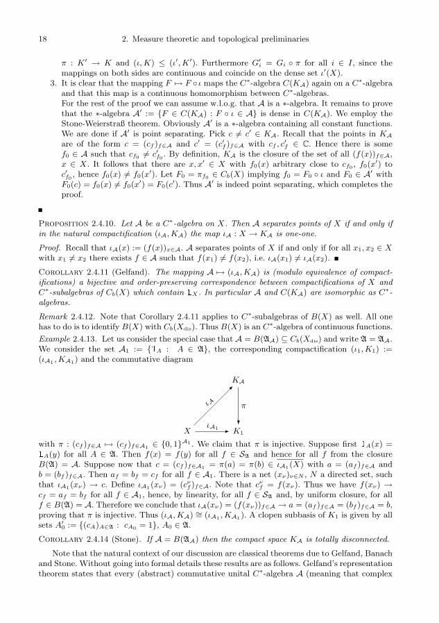
Proposition 2.4.10. Let A be a C∗-algebra on X. Then A separates points of X if and only ifin the natural compactification (ιA,KA) the map ιA : X → KA is one-one.

Proof. Recall that ιA(x) := (f(x))x∈A. A separates points of X if and only if for all x1, x2 ∈ Xwith x1 6= x2 there exists f ∈ A such that f(x1) 6= f(x2), i.e. ιA(x1) 6= ιA(x2).

Corollary 2.4.11 (Gelfand). The mapping A 7→ (ιA,KA) is (modulo equivalence of compact-ifications) a bijective and order-preserving correspondence between compactifications of X andC∗-subalgebras of Cb(X) which contain 1X . In particular A and C(KA) are isomorphic as C∗-algebras.

Remark 2.4.12. Note that Corollary 2.4.11 applies to C∗-subalgebras of B(X) as well. All onehas to do is to identify B(X) with Cb(Xdis). Thus B(X) is an C∗-algebra of continuous functions.

Example 2.4.13. Let us consider the special case that A = B(AA) ⊆ Cb(Xdis) and write A = AA.We consider the set A1 := 1A : A ∈ A, the corresponding compactification (ι1,K1) :=(ιA1 ,KA1) and the commutative diagram

KA

XιA1-

ιA

-

K1

π

?

with π : (cf )f∈A 7→ (cf )f∈A1 ∈ 0, 1A1 . We claim that π is injective. Suppose first 1A(x) =1A(y) for all A ∈ A. Then f(x) = f(y) for all f ∈ SA and hence for all f from the closureB(A) = A. Suppose now that c = (cf )f∈A1 = π(a) = π(b) ∈ ιA1(X) with a = (af )f∈A andb = (bf )f∈A. Then af = bf = cf for all f ∈ A1. There is a net (xν)ν∈N , N a directed set, suchthat ιA1(xν) → c. Define ιA1(xν) = (cνf )f∈A. Note that cνf = f(xν). Thus we have f(xν) →cf = af = bf for all f ∈ A1, hence, by linearity, for all f ∈ SA and, by uniform closure, for allf ∈ B(A) = A. Therefore we conclude that ιA(xν) = (f(xν))f∈A → a = (af )f∈A = (bf )f∈A = b,proving that π is injective. Thus (ιA,KA) ∼= (ιA1 ,KA1). A clopen subbasis of K1 is given by allsets A′0 := (cA)A∈A : cA0 = 1, A0 ∈ A.

Corollary 2.4.14 (Stone). If A = B(AA) then the compact space KA is totally disconnected.

Note that the natural context of our discussion are classical theorems due to Gelfand, Banachand Stone. Without going into formal details these results are as follows. Gelfand’s representationtheorem states that every (abstract) commutative unital C∗-algebra A (meaning that complex

2.5. The Stone-Cech compactification βX 19

conjugation is replaced by an abstract operation with corresponding properties) is isometricallyisomorphic to some C(K) where K is a suitable compact space. In this context K is also calledthe structure space or Gelfand compactum for A. By the Banach-Stone theorem, two compactspaces K1 and K2 are homeomorphic if and only if C(K1) ∼= C(K2) as unital Banach algebras.Furthermore, by Stone’s theorem, for every Boolean algebra B there is a totally disconnectedcompact space K, the so called Stone space associated to B, such that for the systems Cl(K)of all clopen subsets of K we have B ∼= Cl(K) as Boolean algebras. Two such spaces K1 andK2 are homeomorphic if and only if Cl(K1) ∼= Cl(K2). Finally, the Stone space of a Boolean setalgebra A is homeomorphic to the Gelfand compactum for B(A). For the interested reader werefer to [8] and [9].

2.5. The Stone-Cech compactification βX. We now apply the construction of the naturalcompactification for an algebra A, to the case A = Cb(X), i.e. to the algebra of all bounded andcontinuous f : X → C.

Definition 2.5.1. The maximal compactification (ιβ , βX) of a topological space X, correspond-ing to the algebra Cb(X) in the sense on Corollary 2.4.11, is denoted by (ιβ , βX) and is calledthe Stone-Cech compactification of X.

(ιβ , βX) is characterized uniquely up to equivalence by the universal property that for everycontinuous ϕ : X → K, K compact, there is a (unique) continuous ψ : βX → K with ϕ = ψ ιβ .To see this we may w.l.o.g. assume K = ϕ(X) such that (ϕ,K) is a compactification of X. Bythe maximality of (ιβ , βX) and Corollary 2.4.11 this just means that there is a ψ as claimed.For uniqueness assume that (ι,K) is another compactification of X with this universal property.Every f ∈ Cb(X) has a range contained in a compact set K0 ⊆ C. By the universal propertythere is a continuous ψ : K → K0 with ψ ι = f . Hence, again by Corollary 2.4.11 the algebracorresponding to (ι,K) contains Cb(X). Thus (ι,K) has to be maximal, i.e. equivalent (ιβ , βX).

Nevertheless, in order to obtain an interesting and rich structure one needs sufficiently manybounded and continuous functions.

Definition 2.5.2. X is called completely regular if it fulfills the following separation property:For every closed A ⊆ X and x ∈ X \ A there is a continuous f : X → [0, 1] with f(x) = 1 andf(a) = 0 for all a ∈ A. Such an f is called Urysohn function for A and x.

Under this assumption every Urysohn function gives rise to a compactification separatingtwo points x 6= y ∈ X, yielding that ιβ is injective. ιβ is even a homeomorphic embedding ofX into βX. To see this, it suffices to show that for x ∈ O ⊆ X, O open, there is an open setOβ ⊆ βX containing ιβ(x) such that ιβ(O) ⊇ Oβ ∩ ιβ(X). Take a Urysohn function f0 for x andA := X \O, recall that ιβ : x 7→ (f(x))f∈Cb(X) and observe that Oβ := (cf )f∈Cb(X) : cf0 > 0has the required properties.

Let us now consider the case of discrete X, i.e. Cb(X) = B(X). Then each 1A ∈ B(X),A ⊆ X, has a continuous representation in (ιβ , βX) which must be of the form 1A∗ with someclopen A∗ = ιβ(A) ⊆ βX. (Therefore the usual notation A∗ = A as a closure, though notrigorously correct in our setting, does not lead to contradictions.)

Conversely, every clopen set B ⊆ βX can be written as B = A∗ with A := ι−1β [B]. Further-

more such sets form a basis for the topology in βX: Let O ⊆ βX be open and x ∈ O. Then, bythe separation properties of compact spaces, there is an open set Ox such that x ∈ Ox ⊆ Ox ⊆ O.For Ax := ι−1

β [Ox] we obtain x ∈ A∗x ⊆ O. This shows that O =Sx∈O A

∗x can be written as a

union of clopen sets.

Let A = a, a ∈ X, be a singleton and x 6= ιβ(a). There is an open neighborhood O of x notcontaining ιβ(a). Thus the continuous representation of 1A in (ιβ , βX) has to take the constantvalue 0 on O, hence 1A∗ = 1ιβ(a). By continuity this shows that ιβ(a) is open, i.e. ιβ(a) isan isolated point in βX. A further consequence is that A∗∩ ιβ(X \A) = ∅ and A∗∩(X \A)∗ = ∅.


Since

βX = ιβ(X) = ιβ(A) ∪ ιβ(X \A) = ιβ(A) ∪ ιβ(X \A) = A∗ ∪ (X \A)∗

we conclude that Φ : A 7→ A∗ is an isomorphism of Boolean set algebras between P(X), thepowerset of X, and Cl(βX), the system of all clopen sets in βX.

Consider Fx := ι−1β [O] : x ∈ O ⊆ βX,O open. Obviously Fx is a filter on X. For arbitrary

A ⊆ X, by A∗ ∪ (X \ A)∗ = βX, we have either x ∈ A∗ or x ∈ (X \ A)∗. In the first case thismeans A = ι−1

β [A∗] ∈ Fx, in the second case X \ A ∈ Fx. Thus Fx is an ultrafilter. Converselyevery ultrafilter F on X induces an ultrafilter Fβ on βX consisting of all Fβ ⊆ βX which containιβ(F ) for at least one F ∈ F . The compactness of βX guarantees that Fβ converges to somex ∈ βX which is possible only if F = Fx. This shows that the points in βX are in a naturalbijective correspondence with the ultrafilters on X.

We summarize the collected facts about βX.

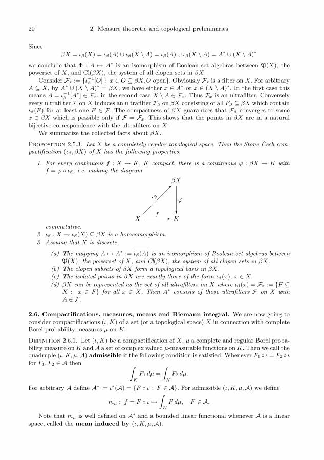
Proposition 2.5.3. Let X be a completely regular topological space. Then the Stone-Cech com-pactification (ιβ , βX) of X has the following properties.

1. For every continuous f : X → K, K compact, there is a continuous ϕ : βX → K withf = ϕ ιβ, i.e. making the diagram

βX

Xf -

ιβ

-

K

ϕ

?

commutative.

2. ιβ : X → ιβ(X) ⊆ βX is a homeomorphism.

3. Assume that X is discrete.

(a) The mapping A 7→ A∗ := ιβ(A) is an isomorphism of Boolean set algebras betweenP(X), the powerset of X, and Cl(βX), the system of all clopen sets in βX.

(b) The clopen subsets of βX form a topological basis in βX.

(c) The isolated points in βX are exactly those of the form ιβ(x), x ∈ X.

(d) βX can be represented as the set of all ultrafilters on X where ιβ(x) = Fx := F ⊆X : x ∈ F for all x ∈ X. Then A∗ consists of those ultrafilters F on X withA ∈ F .

2.6. Compactifications, measures, means and Riemann integral. We are now going toconsider compactifications (ι,K) of a set (or a topological space) X in connection with completeBorel probability measures µ on K.

Definition 2.6.1. Let (ι,K) be a compactification of X, µ a complete and regular Borel proba-bility measure onK andA a set of complex valued µ-measurable functions onK. Then we call thequadruple (ι,K, µ,A) admissible if the following condition is satisfied: Whenever F1 ι = F2 ιfor F1, F2 ∈ A then Z

K

F1 dµ =

ZK

F2 dµ.

For arbitrary A define A∗ := ι∗(A) = F ι : F ∈ A. For admissible (ι,K, µ,A) we define

mµ : f = F ι 7→ZK

F dµ, F ∈ A.

Note that mµ is well defined on A∗ and a bounded linear functional whenever A is a linearspace, called the mean induced by (ι,K, µ,A).

2.6. Compactifications, measures, means and Riemann integral 21

It is clear that for all compactifications (ι,K) of X and all µ we get an admissible quadrupleif we take A := C(K). In this case F1 ι = F2 ι with F1, F2 ∈ A is possible only for F1 = F2

(recall that ι(X) is dense in K). For our subsequent investigations the following similar statementfor A = Rµ is fundamental.

Proposition 2.6.2. For every compactification (ι,K) of X and every complete and regular Borelprobability measure on µ on K the quadruple (ι,K, µ,Rµ) is admissible. Hence

m(F ι) :=

ZK

F dµ

is a well defined mean on the algebra R∗µ.

Proof. W.l.o.g. we may assume that µ has full support, i.e. all nonempty open sets in K havepositive measure. Let f = F1 ι = F2 ι with Fi ∈ Rµ. First we assume that Fi = 1Ai forcertain µ-continuity sets Ai ∈ Cµ. The symmetric difference A := A1 4A2 is a µ-continuity setwith empty interior. We conclude that ∂A ⊆ A has zero measure and hence

R1A1dµ =

R1A2dµ.

By linearity this property extends to functions Fi ∈ SCµ and, using a standard approximationargument, to arbitrary Fi ∈ Rµ.

We have to compare compactifications also in a measure theoretic sense. For this reason wefix further notation.

Definition 2.6.3. Suppose that µi is a complete Borel probability measure on Ki, where (ιi,Ki)is a compactification of X, i = 1, 2. Then we write (ι1,K1, µ1) ≤ (ι2,K2, µ2) if (ι1,K1) ≤ (ι2,K2)via π : K2 → K1 which, in addition to being continuous is also measure preserving, i.e. wheneverA1 ⊆ K1 is µ1-measurable then its pre-image A2 := π−1[A1] is µ2-measurable with µ2(A2) =µ1(A1).

Remark 2.6.4. In the above situation we also could have defined the measure onK1 via µ1(A1) :=µ2(π−1[A1]). This construction is called pullback, and µ1 is often denoted by π µ2.

We know by Proposition 2.4.5 that every f : X → C which has a continuous representationF1 : K1 → C in the compactification (ι1,K1) has a continuous representation F2 := F1 π in(ι2,K2) whenever (ι1,K1) ≤ (ι2,K2) via π : K2 → K1. We get a similar assertion if we replacecontinuity by Riemann integrability.

Proposition 2.6.5. Suppose that f : X → C has a µ1-Riemann integrable representation F1 :K1 → C in the compactification (ι1,K1, µ1). Whenever (ι1,K1, µ1) ≤ (ι2,K2, µ2) via π thenF2 := F1 π is a µ2-Riemann integrable representation of f in (ι2,K2, µ2).

Proof. It is clear that F2 := F1 π is a realization of f whenever F1 is. It is immediate to checkthat disc(F2 π) ⊆ π−1[disc(F1)]. Thus one obtains

µ2(disc(F2) ≤ µ2(π−1[disc(F1)]) = µ1(disc(F1)) = 0.

Thus F2 is µ2-Riemann integrable whenever F1 is µ1-Riemann integrable.

Proposition 2.6.5 shows that (ι1,K1, µ1) ≤ (ι2,K2, µ2) implies F1 ι : F1 ∈ Rµ1 ⊆ F2 ι :F2 ∈ Rµ2. This observation is of particular interest if there exists a maximal (ι,K, µ).

Conversely, assume that a C∗-algebra A of bounded functions f : X → C and a mean m onA is given. Let (ιA,KA) be the natural compactification for A. By Proposition 2.4.9 the mappingι∗ : F → F ι is a bijection between C(KA) and A. Thus m′(F ) := m(F ι) is well definedand a mean on C(KA). By Riesz’ Representation Theorem 2.3.1 m′ induces a Borel probabilitymeasure µ on KA with m′(F ) =

RFdµ for all F ∈ C(KA) which is unique on the σ-algebra

of Borel sets and its µ-completion. So it is not surprising that the m-closure of A contains allf = F ι with F ∈ Rµ.


Proposition 2.6.6. Let A be a C∗-algebra on X and m a mean on A. Let (ιA,KA, µ) be thecompactification where (ιA,KA) is the natural compactification for A and µ is the complete andregular Borel measure on KA which satisfies

RF dµ = m(F ιA) for all F ∈ C(KA). Then

R∗µ := F ιA : F ∈ Rµ ⊆ A(m)

for the m-completion A(m)of A. Furthermore, if A separates points of X, then R∗µ = A(m)

.

Proof. Let F ∈ Rµ, then it is straight-forward to check that F ιA is in the m-closure of A, i.e.

R∗µ ⊆ A(m)

. Assume now that A separates points and take the real-valued function f ∈ A(m). By

definition, for every ε > 0 there are real-valued F1, F2 ∈ C(KA) such that F1 ιA ≤ f ≤ F2 ιAwith

R(F2 − F1)dµ ≤ ε. Observe

F[ := supF1ιA≤f

F1 ≤ F ≤ inff≤F2ιA

F2 =: F#, F1, F2 ∈ C(KA).

The fact that f is in the m-closure of A implies that every F with F[ ≤ F ≤ F# is µ-Riemannintegrable. Since A separates points of X the map ιA : X → KA is one-one, cf. Proposition2.4.10. Thus we can define a function F : KA → R via

F (k) =

f(x)

0

if k = ιA(x)

otherwise.

Then F := maxF , F [ is µ-Riemann integrable and satisfies F ιA = f . Hence R∗µ ⊇ A(m)

.

Remark 2.6.7. In any case R∗µ is a C∗-algebra. ι∗A : F 7→ F ιA is a bounded ∗-homomorphismwhich maps Rµ into B(X) and the image of every bounded ∗-homomorphism is again a C∗-algebra, cf. [8, Theorem I.5.5].

In the general case of a non point-separating algebra A ⊆ B(X) we can do a general con-struction: Consider the equivalence relation on X defined by x ≈ y if for every f ∈ A we havef(x) = f(y). Then A induces an algebra A/≈ ⊆ B(X/≈) which is isomorphic to A but pointseparating.

Example 2.6.8. Let X = a, b, c, A := f : X → C : f(a) = f(b) and consider the fapmδc. Then KA := α, β is a two element set and ιA(a) = ιA(b) =: α. The inclusion A =R∗δβ ⊂ A

mδc = B(X) is strict, showing that in the last statement of Proposition 2.6.6 thepoint-separation property can not be omitted.

However, the identity R∗µ = A(m)may hold even for certain non point separating algebras

A, e.g. if A consists of constant functions.

2.7. The set of all means. For an infinite discrete set X there is an abundance of means onthe algebra B(X) of bounded f : X → C. For a better understanding of the structure of theset of all means, compactifications turn out very useful. We start by restricting to very specialmeans, namely multiplicative ones. (A mean m defined on an algebra A of functions is calledmultiplicative if m(f1 ·f2) = m(f1)m(f2) for all f1, f2 ∈ A.) As a standard reference we mention[17].

Given a multiplicative mean m on B(X), let p = pm be the corresponding fapm, defined onthe whole power set A = P(X) of X. For every A ⊆ X multiplicativity of m yields pm(A) =m(1A) = m(1A · 1A) = m(1A)m(1A) = p2

m(A), hence pm(A) ∈ 0, 1.Conversely, every fapm p defined for all A ⊆ X and taking only the values 0 and 1 induces a

multiplicative mean on B(X): First check that in all four possible cases for p(A1), p(A2) ∈ 0, 1one gets p(A1∩A2) = p(A1)p(A2). This implies mp(f1 · f2) = mp(f1)mp(f2) whenever fi = 1Ai .By multiplicativity and distributivity this transfers to fi ∈ SA. Finally observe that B(X) is theuniform closure of SA to conclude by standard approximation arguments that mp is indeed amultiplicative mean on B(X).

23

Thus multiplicative means are in a one-one correspondence with fapm’s on the power settaking only the values 0 and 1. For an arbitrary such p the system Fp of all A ⊆ X withp(A) = 1 is closed under finite intersections, supersets and contains X, i.e. Fp is a filter. Sincefor each A either p(A) = 1 or p(X \A) = 1, Fp is an ultrafilter. Obviously also this argument isreversible: Every ultrafilter F on X induces a fapm pF by pF (A) = 1F (A) which takes only thevalues 0 and 1. Consider the Stone-Cech compactification βX as the space of ultrafilters on X,according to Proposition 2.5.3. Then the means m on B(X) transfer to positive linear functionalson C(βX) and thus, by Riesz’ Representation Theorem, to Borel probability measures on βX.The functionals, taking only the values 0 and 1, are point evaluations F 7→ F (y), F ∈ C(βX),corresponding to Dirac measures δy concentrated in the point y ∈ βX. As an ultrafilter, ycontains exactly those A ⊆ X with p(A) = 1. Note that, in the set of all sub-probability Borelmeasures, normalized point measures are exactly the extreme ones, i.e. they can be representedas a convex combination only in the trivial way. In the weak-*-topology the set of all sub-probability measures is compact. Thus, by the Krein-Milman Theorem (cf. for instance [40]),an arbitrary Borel measure on βX is in the weak-*-closure of the convex hull of certain pointmeasures. Going back to X and means on X we thus have:

Proposition 2.7.1. The set of all means on B(X), X discrete, is given by the convex hullof all multiplicative means on X. The multiplicative means on X are in a natural bijectivecorrespondence with the points of the Stone-Cech compactification βX.

Indlekofer has systematically used the relation between means and fapm’s on N or Z withprobability measures on the Stone-Cech compactification in probabilistic number theory (cf. forinstance [24]).

In Section 2.4 we have seen that for f : X → C, X discrete, there is a smallest continuousrepresentation which we called the natural one and which is unique up to equivalence. Lookingfor Riemann integrable representations, also a measure has to be involved and thus the situationis more complicated. This has the consequence that there is not one unique (up to equivalence)smallest Riemann integrable representation. Nevertheless, at least for discrete X, one can easilyfind many minimal compactifications:

Example 2.7.2. Let X be discrete. For given bounded f : X → C equip K := f(X) with acompact topology and let ι : x 7→ f(x). Then (ι,K) is a compactification and F : K → C,k 7→ k is the only representation of f in (ι,K). This representation clearly is minimal, providedK carries an appropriate Borel probability measure µ. If K is finite, the discrete topology iscompact and does the job as well as any probability measure µ defined on P(K). In the infinitecase we define a compact topology on K by fixing any k0 ∈ K and taking as open sets all subsetsof K not containing k0 and all cofinite sets which contain k0. Note that all k ∈ K \ k0 areisolated points, hence every function is continuous in such k. The only possible discontinuitypoint is k0. Thus, provided µ(k0) = 0, we have Rµ = B(K). In particular F is µ-Riemannintegrable.

For many reasons this construction is not very satisfactory. One of them is that there is nocanonical choice of µ. The most natural way to find canonical measures is by invariance require-ments. In the forthcoming chapters we will be concerned with invariance mainly with respect togroup or semigroup operations, to some extent also with respect to a single transformation inthe sense of topological and symbolic dynamics.

3. Invariance under transformations and operations

3.1. Invariant means for a single transformation. At the end of the previous chapter wehave seen that there is an abundance of means on an infinite discrete set X. If X carries further

24 3. Invariance under transformations and operations

structure one asks for means and measures with certain interesting additional, namely invarianceproperties.

Definition 3.1.1. Let X be any nonempty set and T : X → X. Then UT : B(X) → B(X)is defined by f 7→ f T . A set A ⊆ B(X) is called T-invariant if UT (A) ⊆ A. Assume thatA is a T-invariant vector space and m is a mean on A. Then m is called T-invariant ifU∗T (m) = UT = m, i.e. if

m(f T ) = m(f)

for all f ∈ A. By M(A) we denote the set of all means on A, M(X) := M(B(X)), and byM(A, T ) the set of all T -invariant m ∈ M(A). For bijective T we call A resp. m two-sidedT-invariant if it is both, T - and T−1-invariant.

Note that in the two sided invariant case one has M(A, T ) = M(A, T−1). It is easy to checkthat M(A) and M(A, T ) are weak-*-closed subsets of the unit ball in B(X)∗, the dual spaceof the Banach space B(X). Thus, since by the Banach-Alaoglu Theorem the dual unit ball iscompact in this topology, M(A) and M(A, T ) are compact as well. More directly, compactnessbecomes clear from applying Tychonoff’s Theorem to

M(A) ⊆Yf∈A

z ∈ C : |z| ≤ ||f ||∞.

As a consequence, any sequence mn ∈M(A) has at least one accumulation point (accumulationmeasure) m ∈M(A). In particular the set MT,(mn) of accumulation means of the sequence (mn)is nonempty:

mn :=1

n

n−1Xk=0

mn(f T k) =1

n

n−1Xk=0

mn(UkT (f)) =1

n

n−1Xk=0

U∗Tk(mn)(f).

Proposition 3.1.2. MT,(mn) ⊆ M(A, T ). In particular there are T -invariant means. We cantake for instance the point evaluation mn := mδx : f 7→ f(x) for any x ∈ X.

Proof. Let m ∈MT,(mn). As m is an accumulation mean, for every ε > 0 and bounded f : X → Cthere is a sequence n1 < n2 < . . . such that both |m(f)−mnk (f)| ≤ ε and |m(f T )−mnk (f T )| ≤ ε for all k ∈ N. From the defining properties of mnk we obtain

|mnk (f T )−mnk (f)| = 1

nk

˛˛nk−1Xj=0

mnk (f T j+1 − f T j)

˛˛

=1

nk|mnk (f Tnk )−mnk (f)| ≤ 2

nk||f ||∞,

|m(f)−m(f T )| ≤ |m(f)−mnk (f)|+ |mnk (f)−mnk (f T )|+ |mnk (f T )−m(f T )|

≤ 2ε+2

nk||f ||∞.

As this is true for all k ∈ N and ε > 0 we obtain T -invariance of m.

We study now which values of m(f) are possible for m ∈M(T,A) and f ∈ A.

Proposition 3.1.3. Let T : X → X, A ⊆ B(X) a T -invariant vector space, f ∈ AR. Then theset m(f) : m ∈M(A, T ) coincides with the interval [a, b] where, with the short hand

a = limn→∞

infx∈X

sn(x) and b = limn→∞

supx∈X

sn(x), sn = sn,T,f :=1

n

n−1Xk=0

f T k. (3.1)

In particular this set does not depend on A.

3.2. Applications 25

Proof. Note first that m(sn) = m(f) for every m ∈ M(A, T ). For the proof it suffices to showthat, for every α ∈ R, there is an m ∈ M(A, T ) with m(f) = α if and only if the followingcondition is satisfied:

Condition(C): For all ε > 0 and n ∈ N there are x = x(ε, n), y = y(ε, n) ∈ X such thatsn(x) > α− ε and sn(y) < α+ ε.

Necessity of (C): Let m(f) = α with m ∈M(A, T ) and suppose, by contradiction, that (C)fails. Then there is an ε > 0 and an n ∈ N such that sn(x) ≤ α − ε for all x ∈ X (the casesn(x) ≥ α+ ε can be treated similarly), hence m(f) = m(sn) ≤ ||sn||∞ ≤ α− ε, contradiction.

Sufficiency of (C): Assume that (C) holds and consider the point measures mn := δx(1/n,n).With the notation of Proposition 3.1.2 this means mn(f) > α− 1

nfor all n. Use Proposition 3.1.2

to find an m′ ∈ MT,(mn) ⊆ M(A, T ). Then m′(f) ≥ α. Similarly one finds an m′′ ∈ M(A, T )with m′′(f) ≤ α. It follows that there is a λ ∈ [0, 1] such that

λm′(f) + (1− λ)m′′(f) = α.

Since M(A, T ) is convex m := λm′ + (1− λ)m′′ has the required properties.

Of particular interest are the functions f with a unique mean value.

Definition 3.1.4. Let T : X → X and A ⊆ B(X) be a T -invariant linear space. A functionf ∈ A is called A-almost convergent if m(f) has the same value for all m ∈ M(A, T ). Theset of all A-almost convergent f ∈ A is denoted by AC(A, T ), for A = B(X) we also writeAC(B(X), T ) = AC(T ). We write mA for the restriction of m ∈ M(A, T ) to AC(A, T ). IfAC(A, T ) = A we call T uniquely ergodic (with respect to A).

By definition, mA does not depend on m. It is clear that AC(A, T ) is a T -invariant uniformlyclosed linear space containing all constant functions. Furthermore AC(A, T ) = AC(T ) ∩ A.Finally, f ∈ AC(A, T ) with mA(f) = α if and only if f ∈ A and, for all xn ∈ X,

limn→∞

sn,T,f (xn) =1

n

n−1Xk=0

f(T k(xn)) = α.

The obvious way to define T -invariance of a set algebra A on X or a finitely additive measure pdefined on A is to require that 1A : A ∈ A ⊆ B(X) resp. mp as defined in Section 2.2 is T -invariant. Since 1AT = 1T−1[A] this is the case if and only if T−1[A] ∈ A resp. p(T−1[A]) = p(A)for all A ∈ A. From Proposition 3.1.3 we get:

Proposition 3.1.5. The possible values p(A) for T -invariant fapm p are given by the interval[a, b] where

a = limn→∞

infx∈X

dn(x) and b = limn→∞

supx∈X

dn(x), dn(x) =1

n

˛k : T k(x) ∈ A, 0 ≤ k < n

˛.

In particular, p(A) takes the same value for all T -invariant p if and only if a = b.

3.2. Applications.

3.2.1. Finite X. Let X be finite, T : X → X and A = B(X) = CX . For every x ∈ Xthere is a minimal m ≥ 0 and a minimal k > n such that T k(x) = Tm(x). We call Cx :=Tm(x), Tm+1(x), . . . , T k−1(x) the cycle (cyclic attractor) induced by x and Bx = B(Cx) :=y ∈ X : Cy = Cx the basin of Cx. It is clear that Cx ⊆ Bx, the Bx forming a partition.Cx = Bx if and only if the restriction of T to this set is bijective. Furthermore the sn = sn,T,fdefined by

sn(x) =1

n

n−1X1

f(T k(x))


converge to a function f which, on each C = Cx, takes the constant value

mC(f) :=1

|C|Xy∈C

f(y).

It is clear that mC ∈M(B(X), T ) for each cycle C. The same holds for all convex combinations.We claim that, conversely, every m ∈ M(B(X), T ) is of this type, i.e. m =

PC λCmC with

0 ≤ λC ≤ for all C andPC λC = 1. To see this, define λC := m(1B(C)) and observe that

f =XC

mC(f)1B(C).

This implies

m(f) = m(sn) = m(f) =XC

mC(f)m(1B(C)) =XC

λCmC(f).

The uniqueness of the λC follows since the mC are linearly independent. This gives an obviousdescription of almost convergent functions: f ∈ AC(B(X), T ) if and only if mC(f) takes thesame value for all cycles C.

In terms of measures this means that every T -invariant p is a convex combination of theergodic measures pC defined by pC(A) := |A∩C|

|C| . This is the finite version of the ergodic decom-

position given by Birkhoff’s Ergodic Theorem (cf. for instance [55]). Infinite X would have tobe treated in this context, but we do not go further into this direction.

3.2.2. X = Z, T : x 7→ x+ 1. First note that whenever A ⊆ B(Z) is two sided T -invariant thenT -invariance of a mean m or a fam p implies invariance with respect to all translations on theadditive group Z. In Section 3.6 we will focus on this aspect. Here we want to apply our analysisfrom Section 3.1. For this reason we have to consider the quantities

sN,f (n) :=1

N

n+N−1Xk=n

f(k)

and, for real valued f , the corresponding lower and upper limits

m∗(f) := limN→∞

infn∈Z

sN,f (n) and m∗(f) := limN→∞

supn∈Z

sN,f (n).

For f = 1A these values m∗(A) := m∗(1A) and m∗(A) := m∗(1A) are known as lower Banachdensity resp. upper Banach density of A. The possible values of T -invariant measures aregiven by

m(f) : m ∈M(T,A) = [m∗(f),m∗(f)],

henceAC(A, T ) = f ∈ A : m∗(f) = m∗(f).

The restriction of m∗ and m∗ to AC(Z) := AC(B(X), T ) is known as Banach density anddenoted by mB .

We have already mentioned that the set AC(Z) of almost convergent f on Z is a linear spaceand, furthermore, uniformly closed. Having the results about compactifications and complexvalued functions in mind, we ask whether AC(Z) is an algebra as well. But this is not the caseas the following example shows.

Example 3.2.1. Consider the sets A = 2Z of even numbers and B = (B1 ∪ B2) ∪ (−B1 ∪ −B2)with

B1 =

∞[n=1

((2n− 1)!, (2n)!] ∩ 2Z,

B2 =

∞[n=1

((2n)!, (2n+ 1)!] ∩ (2Z + 1).

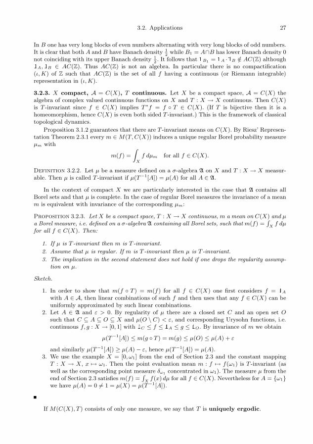
3.2. Applications 27

In B one has very long blocks of even numbers alternating with very long blocks of odd numbers.It is clear that both A and B have Banach density 1

2while B1 = A∩B has lower Banach density 0

not coinciding with its upper Banach density 12. It follows that 1B1 = 1A ·1B /∈ AC(Z) although

1A,1B ∈ AC(Z). Thus AC(Z) is not an algebra. In particular there is no compactification(ι,K) of Z such that AC(Z) is the set of all f having a continuous (or Riemann integrable)representation in (ι,K).

3.2.3. X compact, A = C(X), T continuous. Let X be a compact space, A = C(X) thealgebra of complex valued continuous functions on X and T : X → X continuous. Then C(X)is T -invariant since f ∈ C(X) implies T ∗f = f T ∈ C(X). (If T is bijective then it is ahomeomorphism, hence C(X) is even both sided T -invariant.) This is the framework of classicaltopological dynamics.

Proposition 3.1.2 guarantees that there are T -invariant means on C(X). By Riesz’ Represen-tation Theorem 2.3.1 every m ∈M(T,C(X)) induces a unique regular Borel probability measureµm with

m(f) =

ZX

f dµm for all f ∈ C(X).

Definition 3.2.2. Let µ be a measure defined on a σ-algebra A on X and T : X → X measur-able. Then µ is called T -invariant if µ(T−1[A]) = µ(A) for all A ∈ A.

In the context of compact X we are particularly interested in the case that A contains allBorel sets and that µ is complete. In the case of regular Borel measures the invariance of a meanm is equivalent with invariance of the corresponding µm:

Proposition 3.2.3. Let X be a compact space, T : X → X continuous, m a mean on C(X) and µa Borel measure, i.e. defined on a σ-algebra A containing all Borel sets, such that m(f) =

RXf dµ

for all f ∈ C(X). Then:

1. If µ is T -invariant then m is T -invariant.

2. Assume that µ is regular. If m is T -invariant then µ is T -invariant.

3. The implication in the second statement does not hold if one drops the regularity assump-tion on µ.

Sketch.

1. In order to show that m(f T ) = m(f) for all f ∈ C(X) one first considers f = 1A

with A ∈ A, then linear combinations of such f and then uses that any f ∈ C(X) can beuniformly approximated by such linear combinations.

2. Let A ∈ A and ε > 0. By regularity of µ there are a closed set C and an open set Osuch that C ⊆ A ⊆ O ⊆ X and µ(O \ C) < ε, and corresponding Urysohn functions, i.e.continuous f, g : X → [0, 1] with 1C ≤ f ≤ 1A ≤ g ≤ 1O. By invariance of m we obtain

µ(T−1[A]) ≤ m(g T ) = m(g) ≤ µ(O) ≤ µ(A) + ε

and similarly µ(T−1[A]) ≥ µ(A)− ε, hence µ(T−1[A]) = µ(A).3. We use the example X = [0, ω1] from the end of Section 2.3 and the constant mapping

T : X → X, x 7→ ω1. Then the point evaluation mean m : f 7→ f(ω1) is T -invariant (aswell as the corresponding point measure δω1 concentrated in ω1). The measure µ from theend of Section 2.3 satisfies m(f) =

RXf(x) dµ for all f ∈ C(X). Nevertheless for A = ω1

we have µ(A) = 0 6= 1 = µ(X) = µ(T−1[A]).

If M(C(X), T ) consists of only one measure, we say that T is uniquely ergodic.


Corollary 3.2.4. Let M(C(X), T ) = m. For every f ∈ C(X)

sn,T,f (x) :=1

n

n−1Xk=0

f(T k(x))→ m(f), uniformly in x ∈ X,

in particular, the uniform closure of the convex hull of the T -orbit contains the constant functionm(f) · 1X .

Proof. By Proposition 3.1.3 we know that

limn→∞

„infx∈X

sn,T,f (x)

«= m(f) = lim

n→∞

„supx∈X

sn,T,f (x)

«,

i.e. for every ε > 0 and large enough n we have supx∈X |sn,T,f (x)−m(f)| < ε.

If T is uniquely ergodic, m(f)1X is the only constant function in the uniform closure of theconvex hull of the T -orbit. For a arbitrary constant λ ∈ C in this closure we have

λ = m(λ1X) = limk→∞

m(f Tnk ) = m(f), whenever f Tnk → λ1X .

3.2.4. Shift spaces and symbolic dynamics. We now consider a special case of the situationtreated in Section 3.2.3. Let A be a finite set. In this context A is called an alphabet and itsmembers are called symbols. Furthermore let X be a closed subset of the compact space AZ

which is shift invariant, i.e. σ(X) = X for the shift σ : (ak)k∈Z 7→ (ak+1)k∈Z. Such dynamicalsystems (X,σ) are also called subshifts and are the main objects of symbolic dynamics.

The importance of this apparently simple objects is due to the abundance of σ-invariantclosed subsets X of AZ by which a quite big class of dynamical systems can be represented ina reasonable way. Assume that Y is a compact space, T : Y → Y a continuous transformation,Y = Y0 ∪ Y1 ∪ . . . ∪ Ys−1 (pairwise disjoint union), s ∈ N, a finite partition of Y and F : Y →0, 1, . . . , s− 1, y 7→ i if y ∈ Yi.

Note that F is in general (in particular for connected Y ) not continuous but, if the Yi arecontinuity sets w.r.t. an appropriate measure on Y , Riemann integrable. Therefore we must notexpect that the induced mapping y 7→ x(y) := (F (T ky))k∈Z is continuous. But we may considerthe closure X of its image which is shift invariant. In many interesting cases of a metrizable Ythere is a continuous surjection ϕ : X → Y such that y = ϕ(x) whenever x = x(y). One saysthat (Y, T ) is a factor of (X,σ) and we have the following commutative diagram

Xϕ - Y

X

σ

? ϕ - Y.

T

?

Example 3.2.5 (Sturmian sequence). Let Y = R/Z, α ∈ Y and T be the homeomorphismy 7→ y + α (rotation). Consider the partition of Y into two segments Y0 = [0, α) + Z andY1 = [α, 1) + Z. Hence A = 0, 1. For the T -orbit x(0) of y = 0, i.e. x(0) = (ak)k∈Z withak = 1 if kα ∈ Y1 and ak = 0 if kα ∈ Y0 it turns out that X is the closure of the shift orbitσk(x(0)) : k ∈ Z in 0, 1Z of x(0) in 0, 1Z. The two sided sequence x(0) is an example of aso called Sturmian sequence, a class providing some of the most simple but typical examples ofHartman functions, the main topic of the forthcoming chapters.

In order to understand invariant means or, equivalently by Riesz’ Representation Theorem2.3.1 and Proposition 3.2.3, invariant measures on shift spaces X ⊆ AZ, note that every invariantBorel probability measure on X is uniquely determined by its values on cylinder sets S =[b0, . . . , bn−1] = (ak)k∈Z : ak = bk, k = 0, . . . , n − 1. Thus it suffices to consider functionsf = 1S for such S and apply the arguments from Section 3.1. For instance the numbers a, b

3.3. Compactifications for transformations and actions 29

in Proposition 3.1.3 can be described in terms of relative frequencies of blocks (b0, . . . , bn−1) insymbolic sequences x ∈ X.

3.2.5. The free group F (x, y). Let X = F (x, y) denote the group with two free generators xand y. As usual we assume each member w ∈ F (x, y) to be a reduced word built up from thefour allowed symbols x, y, x−1, y−1, including the empty word w = ∅. Denote by Wx all reducedwords ending with the symbol x; Wx−1 ,Wy and Wy−1 are defined analogously. Consider thetransformation T1 : w 7→ wx−1. In particular we have T1(Wx) = Wx ∪Wy ∪Wy−1 ∪∅. Assumem1 ∈M(T1, B(X)). Then, for the associated fapm p1 = mp1 we compute

0 = p1(T1(Wx))− p1(Wx) = p1(Wy ∪Wy−1 ∪ ∅). (3.2)

By symmetry, for T2 : w 7→ wy−1 we have T2(Wy) = Wy ∪Wx ∪Wx−1 ∪ ∅ and every m2 ∈M(T2, B(X)) satisfies

0 = p2(T2(Wy))− p2(Wy) = p2(Wx ∪Wx−1 ∪ ∅). (3.3)

In particular we have T1(Wx)\Wx∪T2(Wy)\Wy = X. Assume m ∈M(T1, B(X))∩M(T2, B(X)).The associated fapm p = mp satisfies

1 = p(X) = p (T1(Wx) \Wx ∪ T2(Wy) \Wy) (3.4)

≤ p(T1(Wx))− p(Wx) + p(T2(Wy))− p(Wy) = 0, (3.5)

contradiction. Thus there is no mean on B(X) which is both T1- and T2-invariant.Since T1 and T2 are group translations this shows that X = F (x, y) is not an amenable

group, see also Section 3.6.4. Together with the fact that F (x, y) can be realized as a group oforthogonal transformations of R3 this is the core of the celebrated Banach-Tarski paradox, see[54]. We will focus on (semi-)group structures systematically in Section 3.6.

3.3. Compactifications for transformations and actions. We have seen the importanceof compactifications for means and measures already in Chapter 2. The role of transformationsfor identifying interesting measures in terms of invariance properties was pointed out in Section3.1. We now combine both points of view by investigating the following setting.

Definition 3.3.1. Let X be a topological space, T : X → X continuous and (ι,K) a com-pactification of X. Then (ι,K) is called a compactification compatible with T and, vice versa,T a transformation compatible with (ι,K) if there is a continuous TK : K → K such thatι T = TK ι, i.e. making the diagram

Xι - K

X

T

? ι - K.

TK

?

commutative. TK is called a continuous extension of T in (ι,K).

Continuous extensions are unique and compatible with composition:

Proposition 3.3.2. Let TK and T ′K be continuous extensions of T : X → X in the compactifi-cation (ι,K) of X. Then TK = T ′K . Furthermore, if SK is a continuous extension of S : X → Xin (ι,K) then (S T )K = SK TK : K → K, is the continuous extension of S T : X → X.

Proof. The first statement follows since TK and T ′K are continuous and coincide on the denseset ι(X) ⊆ K. For the second statement observe

(SK TK) ι = SK (TK ι) = SK (ι T )

= (SK ι) T = (ι S) T = ι (S T )


and use the uniqueness of continuous extensions to obtain SK TK = (S T )K .

Note that from a certain point of view for continuous extensions of transformations T : X →X the situation is more complicated than for representations of complex valued f : X → C inthe sense of Section 3.5. This is due to the fact that there is no obvious analogue of Proposition2.4.9 which yields a natural compactification for f or even for a unital C∗-algebra A which isminimal. Proposition 2.4.9 was based on Proposition 2.4.5 yielding that for each compactifica-tion allowing a continuous representation every bigger compactification has the same property.The following example shows that this is not true for T : X → X.

Example 3.3.3. Let X = Z, T : k 7→ k + 1, α ∈ R \ Q, and consider the compactifications(ιi,Ki), i = 1, 2, given by K1 := T = R/Z, ι1 : k 7→ kα + Z, and K2 := [0, 1], ι2 : k 7→ kα :=kα − maxm ∈ Z : m ≤ kα. Obviously (ι1,K1) ≤ (ι2,K2) via π : K2 = [0, 1] → R/Z = K2,x 7→ x + Z. The compactification (ι1,K1) is compatible with T since T1 : x 7→ x + α is acontinuous extension of T in (ι1,K1). There is no continuous extension T2 of T in (ι2,K2). Letus prove this by contradiction, i.e. by assuming that such a T2 : [0, 1]→ [0, 1] exists. Since ι2(Z)is dense in [0, 1] we can find a sequence xn = knα = ι2(kn) such that xn → 1−α. Furthermorewe can arrange 0 ≤ xn < 1− α for all n ∈ N. Using T2 ι2 = ι2 T we get

T2(1− α) = limn→∞

T2(xn) = limn→∞

T2 ι2(kn) = limn→∞

ι2 T (kn) =

= limn→∞

ι2(kn + 1) = limn→∞

knα+ α = limn→∞

xn + α = 1.

We now pick another sequence yn = lnα = ι2(ln) such that yn → 1 − α but now with therequirement 1− α < yn ≤ 1 for all n ∈ N. Similarly, we get

T2(1− α) = limn→∞

T2(yn) = limn→∞

T2 ι2(ln) = limn→∞

ι2 T (ln) =

= limn→∞

ι2(ln + 1) = limn→∞

lnα+ α = limn→∞

yn + α− 1 = 0,

contradiction.

We see that taking bigger compactifications does not guarantee that we find continuousextensions. Nevertheless, for the Stone-Cech compactification (ιβ , βX), cf. Section 2.5, everythingworks. In particular the first statement of Proposition 2.5.3 applies to K = βX: For everycontinuous T : X → X the map ιβ T : X → βX is continuous. Therefore there is a continuousTβ : βX → βX such that Tβ ιβ = ιβ T .

Definition 3.3.4. Let X be a completely regular space and T : X → X be continuous. Then Tβ :βX → βX denotes the (unique) continuous extension of T in the Stone-Cech compactification(ιβ , βX) of X.

There is no obstacle to consider families of transformations instead of a single T . In order toproceed into this direction recall the notion of (semi)group actions.

Definition 3.3.5. Let S be a semigroup and X a set. A mapping α : S×X → X,(s, x) 7→ α(s, x)is called a semigroup action of S on X if α(s1, s2(x)) = α(s1s2, x) for all s1, s2 ∈ S and allx ∈ X.

This construction carries over in the obvious way to groups:

Definition 3.3.6. LetG be a semigroup andX a set. A mapping α : G×X → X,(g, x) 7→ α(g, x)is called a group action of G on X if it is a semigroup action of G considered as a semigroupand α(eG, x) = x, for the unit element eG ∈ G and all x ∈ X.

For a semigroup action the maps sα : x 7→ α(s, x) are self-maps of X. If we impose asemigroup structure on XX , the set of all maps f : X → X, by using the composition of mapsas semigroup operation, a semigroup action of S on X is nothing else than a homomorphism

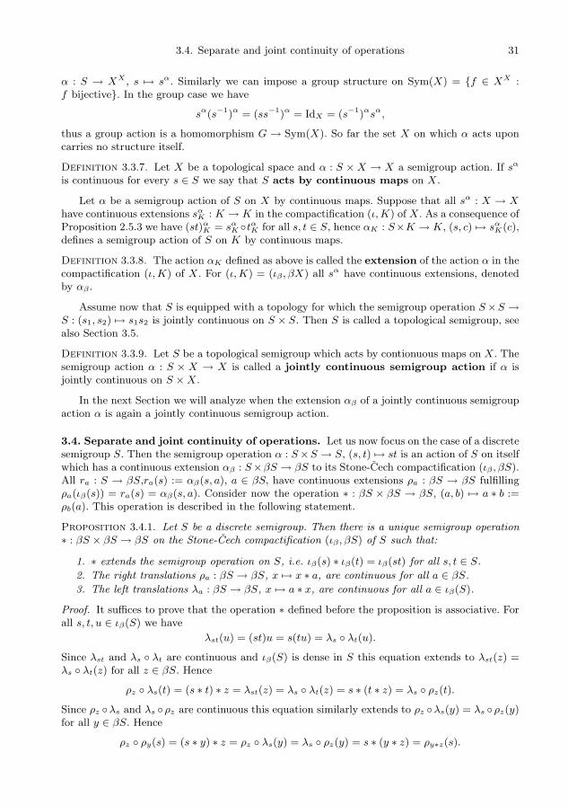
3.4. Separate and joint continuity of operations 31

α : S → XX , s 7→ sα. Similarly we can impose a group structure on Sym(X) = f ∈ XX :f bijective. In the group case we have

sα(s−1)α = (ss−1)α = IdX = (s−1)αsα,

thus a group action is a homomorphism G → Sym(X). So far the set X on which α acts uponcarries no structure itself.

Definition 3.3.7. Let X be a topological space and α : S ×X → X a semigroup action. If sα

is continuous for every s ∈ S we say that S acts by continuous maps on X.

Let α be a semigroup action of S on X by continuous maps. Suppose that all sα : X → Xhave continuous extensions sαK : K → K in the compactification (ι,K) of X. As a consequence ofProposition 2.5.3 we have (st)αK = sαK tαK for all s, t ∈ S, hence αK : S×K → K, (s, c) 7→ sαK(c),defines a semigroup action of S on K by continuous maps.

Definition 3.3.8. The action αK defined as above is called the extension of the action α in thecompactification (ι,K) of X. For (ι,K) = (ιβ , βX) all sα have continuous extensions, denotedby αβ .

Assume now that S is equipped with a topology for which the semigroup operation S×S →S : (s1, s2) 7→ s1s2 is jointly continuous on S × S. Then S is called a topological semigroup, seealso Section 3.5.

Definition 3.3.9. Let S be a topological semigroup which acts by contionuous maps on X. Thesemigroup action α : S × X → X is called a jointly continuous semigroup action if α isjointly continuous on S ×X.

In the next Section we will analyze when the extension αβ of a jointly continuous semigroupaction α is again a jointly continuous semigroup action.

3.4. Separate and joint continuity of operations. Let us now focus on the case of a discretesemigroup S. Then the semigroup operation α : S×S → S, (s, t) 7→ st is an action of S on itselfwhich has a continuous extension αβ : S×βS → βS to its Stone-Cech compactification (ιβ , βS).All ra : S → βS,ra(s) := αβ(s, a), a ∈ βS, have continuous extensions ρa : βS → βS fulfillingρa(ιβ(s)) = ra(s) = αβ(s, a). Consider now the operation ∗ : βS × βS → βS, (a, b) 7→ a ∗ b :=ρb(a). This operation is described in the following statement.

Proposition 3.4.1. Let S be a discrete semigroup. Then there is a unique semigroup operation∗ : βS × βS → βS on the Stone-Cech compactification (ιβ , βS) of S such that:

1. ∗ extends the semigroup operation on S, i.e. ιβ(s) ∗ ιβ(t) = ιβ(st) for all s, t ∈ S.

2. The right translations ρa : βS → βS, x 7→ x ∗ a, are continuous for all a ∈ βS.

3. The left translations λa : βS → βS, x 7→ a ∗ x, are continuous for all a ∈ ιβ(S).

Proof. It suffices to prove that the operation ∗ defined before the proposition is associative. Forall s, t, u ∈ ιβ(S) we have

λst(u) = (st)u = s(tu) = λs λt(u).

Since λst and λs λt are continuous and ιβ(S) is dense in S this equation extends to λst(z) =λs λt(z) for all z ∈ βS. Hence

ρz λs(t) = (s ∗ t) ∗ z = λst(z) = λs λt(z) = s ∗ (t ∗ z) = λs ρz(t).

Since ρz λs and λs ρz are continuous this equation similarly extends to ρz λs(y) = λs ρz(y)for all y ∈ βS. Hence

ρz ρy(s) = (s ∗ y) ∗ z = ρz λs(y) = λs ρz(y) = s ∗ (y ∗ z) = ρy∗z(s).


Once again, since ρz ρy and ρy∗z are continuous this equation extends to ρz ρy(x) = ρy∗z(x)for all x ∈ βS, hence

(x ∗ y) ∗ z = ρz ρy(x) = ρy∗z(x) = x ∗ (y ∗ z)

for all x, y, z ∈ βS.

For much more information about the algebraic structure of βS we refer to [23]. There onecan also find information about related constructions as the enveloping semigroup of a semigroupof continuous transformations etc. We are now going to show that ∗ is jointly continuous onlyin very special cases (which are not strikingly interesting). Not for maximizing generality but inorder to identify the natural context we use terminology from General Algebra.

Definition 3.4.2. For any set X, a function ω : Xn → X, n ∈ N, is called an n-ary operationon X. If (ι,K) is a compactification of X, ωK : Kn → K is called an extension of ω ifιω = ωK ιn with ιn : Xn → Xn, (x1, . . . , xn) 7→ (ι(x1), . . . , ι(xn)). (ι,K) is called compatiblewith ω and vice versa if a continuous extension ωK of ω exists.

Remark 3.4.3. If ω0 is an m-ary operation on X and ω1, . . . , ωm are n-ary operations on X thenω(x1, . . . , xn) := ω0(ω1(x1, . . . , xn), . . . , ωm(x1, . . . , xn)) defines an n-ary operation ω on X,called the composition of ω0 and the ωi, i = 1, . . . ,m. If all involved operations are continuousthen so is ω. Other (trivial) examples of continuous n-ary operations are the projections πni :(x1, . . . , xn) 7→ xi, 1 ≤ i ≤ n. A set Ω of operations on X which contains all projections and isclosed under composition is called a clone on X. Thus, for every family of continuous ni-aryoperations ωi on X, i ∈ I, all operations in the clone generated by the ωi are continuous as well.A standard reference on the clone of continuous functions is [50]. From this point of view thetraditional approach in General Algebra, namely to define a universal algebra as an object ofthe type (X, (ωi)i∈I), is intimately connected with the investigation of clones. In particular forinfinite X there is indeed much current research on clones on X, cf. [16]. But here we proceedin a different direction.

Recall that, by definition, a topological space is 0-dimensional if there exists a topologicalbasis of clopen sets.

Lemma 3.4.4. Let X be a 0-dimensional compact Hausdorff space and R ⊆ Xn a clopen subset.Then R =

Ski=1Ri is a finite union of generalized rectangles Ri = Ai,1 × . . .× Ai,n with clopen

Ai,j ⊆ X,i = 1, . . . , k, j = 1, . . . , n. The Ri can be taken pairwise disjoint and such that all theAi,j are from a fixed finite partition P = A1, . . . , Ak.

Proof. Pick x = (x1, . . . , xn) ∈ R. Since R is open and X has a clopen basis there are clopenneighborhoods Ax,i of xi such that Ax := Ax,1 × . . . × Ax,n ⊆ R. Hence R =

Sx∈RAx. This

covering is open. Since R, being a closed subset of X, is compact, finitely many Ri := Axi ,i = 1, . . . , k, form a covering as well. It is clear that by finite refinements, the Ri can be takenpairwise disjoint and all the resulting Ai,j from one finite partition.

This lemma yields a characterization of operations having a continuous extension in theStone-Cech compactification.

Theorem 1. Let X be discrete and ω : Xn → X an n-ary operation on X. Then ω has acontinuous extension in the Stone-Cech compactification (ιβ , βX) if and only if for every S ⊆ Xthe preimage is a finite union of rectangles, i.e.

ω−1[S] =

k[i=1

Ri with Ri = Ai,1 × . . .×Ai,n.

Proof. Necessity of the condition: Assume that ωβ is the continuous extension of ω in (ιβ , βX).S∗ = ιβ(S) (notation as in Proposition 2.5.3) is clopen, hence, by continuity of ωβ , ω−1

β [S∗] is

3.5. Compactifications for operations 33

clopen as well. So Lemma 3.4.4 applies, yielding that this set is a finite union of rectangles. Thisimmediately translates to the same property of ω−1[S].

Sufficiency of the condition: Assume that for ω : Xn → X all preimages ω−1[S], S ⊆ X, arefinite unions of rectangles. We have to construct a continuous extension ωβ of ω in (ιβ , βX). Weuse the ultrafilter description from Proposition 2.5.3. So let p1, . . . , pn be ultrafilters on X. Wedefine an ultrafilter p := ωβ(p1, . . . , pn) on X by letting F ⊆ X be a member of p if and only ifω(F1× . . .×Fn) ⊆ F for some sets Fi ∈ pi. It is straight forward to check that ∅ /∈ p, that F ∈ pand F ⊆ F ′ ⊆ X implies F ′ ∈ p and that F, F ′ ∈ p implies F ∩ F ′ ∈ p. But p is even maximal:For arbitrary F ⊆ X our assumption yields that R := ω−1[F ] can be taken as stated in Lemma3.4.4. Since for each j = 1, . . . , n, pj is an ultrafilter on X there is exactly one Akj ∈ p such thatAkj ∈ pj . For the rectangle R′ := Ak1 × . . .×Akn we either have R′ ⊆ R or R′ ⊆ X \R. In thefirst case this implies F ∈ p, in the second case X \ F ∈ p, showing that p is an ultrafilter.

Finally we have to prove that ωβ is continuous on (βX)n. We use Proposition 2.5.3 severaltimes. Take arbitrary ultrafilters p1, . . . , pn ∈ βX and any neighborhood U of p := ωβ(p1, . . . , pn).By the definition of the topology on βX there is a set F ⊆ X such that F ∈ p1 and U contains allultrafilters p with F ∈ p. By the definition of ωβ there are Fi ∈ pi such that ω(F1×. . .×Fn) ⊆ F .Each Fi defines a neighborhood Ui of pi consisting of all ultrafilters which contain Fi. It is clearthat ωβ(U1 × . . .× Un) ⊆ U , showing that ωβ is continuous.

Corollary 3.4.5. Let S be an infinite discrete group. Then there is no continuous extension ofthe group operation on S in (ιβ , βS).

Proof. Preimages of singletons are infinite but contain only singleton rectangles, thus can notbe finite unions of rectangles.

Similar arguments apply for many semigroups as N with addition or with multiplication orinfinite totally ordered sets with min or max as semigroup operation.

Definition 3.4.6. An n-ary operation ω : Xn → X is called essentially unary (dependingon the i-th component) if there is an f : X → X such that ω(x1, x2, . . . , xn) = f(xi) for allx1, . . . , xn ∈ Xn. ω is called locally essentially unary if there is a finite partition of X intosets Ai, i = 1, 2, . . . , k, such that the restriction of f to each rectangle R = Ai1 × . . . × Ain ,ij ∈ 1, 2, . . . , k is essentially unary.

Proposition 3.4.7. Let ω : Xn → X be locally essentially unary. Then there is a continuousextension ωβ of ω to (ιβ , βX).

Proof. As the reader checks easily, every locally unary operation ω satisfies the condition ofTheorem 1.

Continuing work of van Douwen [52], Farah was able to show in [10, 11] that the converseof Proposition 3.4.7 also holds true.

Proposition 3.4.8 (Farah). Let X be an infinite discrete set and assume that ω : Xn → X hasa continuous extension in (ιβ , βX). Then ω is locally essentially unary.

3.5. Compactifications for operations. We have seen in the previous section that manyinteresting binary operations can not be extended continuously to the Stone-Cech compactifi-cation. Nevertheless some ideas presented in Section 2.4 can be adapted. In order to be moreflexible it is useful to consider the following setting.

Definition 3.5.1. Let I be an index set, ni ∈ N and γi ⊆ P(1, 2, . . . , ni) for all i ∈ I. A semi-topological (general) algebra of type τ = ((ni)i∈I , (γi)i∈I) is a topological space X togetherwith a family of ni-ary operations ωi : Xni → X for which (xj1 , . . . , xjs) 7→ ωi(x1, . . . , xni) iscontinuous for all j1, . . . , js ∈ γi and all fixed xi ∈ X, i /∈ j1, . . . , js. This semitopologicalalgebra is called a topological algebra if furthermore 1, . . . , ni ∈ γi for all i ∈ I. In this caseone might omit the information contained in the γi and consider τ to be given by the τ = (ni)i∈I .


Example 3.5.2 (Semitopological algebras).• Topological groups are groups considered as topological algebras of type τ = (2, 1), re-

quiring joint continuity of the binary operation as well as continuity of the operationx 7→ x−1.

• Topological groups can also be seen as topological algebras of type τ = (2, 1, 0) if oneprefers to emphasize that the neutral element may be considered as a 0-ary operation.

• Topological semigroups are semigroups which are topological algebras of type τ = (2).

• Semitopological semigroups are semigroups considered as semitopological algebras of type(2, 1, 2), i.e. the semigroup operation is continuous in each component but notnecessarily jointly continuous. Similarly the type of left and right topological semigroupsis τ = (2, γ) with γ = i with i = 1 resp. i = 2.

The value of the rather technical concept of a semitopological algebra gets clear by consid-ering compactifications of general algebras.

Definition 3.5.3. Let X and K be (semi)topological algebras of type τ . If (ι,K) is a compact-ification of the set X such that each operation on K extends the corresponding operation on Xwe call (ι,K) a τ-compactification of X. In the case of topological groups, (semi)topologicalsemigroups etc. these compactifications are also called group, (semi)topological (semi)group etc.compactifications in the obvious way.

Later we will discuss the special cases of group, semigroup and semitopological semigroupcompactifications in more detail. In the general context the following observations hold.

Proposition 3.5.4.1. The direct product of a family of (semi)topological algebras of type τ is again a (semi)topo-

logical algebra of type τ .

2. Every (semi)topological algebra of type τ has a maximal τ -compactification.

Proof. The first statement is obvious. For the second statement the product compactification, cf.Definition 2.4.6, of all (semi)topological compactifications of type τ has the required properties.To justify this construction it suffices to show that there is a set S of compactifications of Xsuch that for every τ -compactification (ι,K) of X there is an equivalent compactification in S.Since |K| ≤ |βX| one can take for S the set of all compactifications (ι,K) of X with K ⊆ βX(as a set, not necessarily as a topological subspace or subalgebra).

Example 3.5.5.1. For a topological group G the maximal group compactification is called the almost periodic

or Bohr compactification and denoted by (ιb, bG).

2. For a semitopological semigroup S the maximal semitopological semigroup compactifica-tion is called the weak almost periodic compactification and denoted by (ιw, wS),see also Section 4.2. For the realization of wS as space of filters in the spirit of Proposition2.5.3 we refer to [4].

3.6. Invariance on groups and semigroups.

3.6.1. The action of a semigroup by translations. With every (semi)group S comes anatural action, namely the action of S by right translations.

Definition 3.6.1. Let S be a semitopological semigroup. Then S acts on B(S) by right trans-lations in the following way (notation as in Proposition 3.4.1):

R : S ×B(S)→ B(S), Rs(f)(t) := f(ρs(t)) = f(ts).

For every s ∈ S the map Rs is a bounded linear operator. As for the left translations

L : S ×B(S)→ B(S), Ls(f)(t) := f(λs(t)) = f(st)

3.6. Invariance on groups and semigroups 35

we have LsLt = Lts the map (s, f) 7→ Lf is not a semigroup action, but merely an ”anti”-actionof S on B(S). However, in the group case we can define an action Λ : G × B(G) → B(G) viaΛs(f)(t) = f(λs−1t) after all.

In the sequel we use compatibility with respect to these translations to single out a uniquemeasure or mean on certain algebras A ⊆ B(S). We will mainly focus on the group case. As incontrast to the previous sections this section will be less self-contained. As standard references(which also extensively treat the semigroup case) we mention [5, 6, 18, 34, 39, 40, 41].

3.6.2. Means.

Definition 3.6.2. Let A ⊆ B(S) be a ∗-algebra which is invariant under translations. A meanm ∈M(A) is left (right) invariant, if m(f) = m(Lsf) (m(f) = m(Rsf)) for all s ∈ S and f ∈ A.A mean which is both left and right invariant is called bi-invariant, or, simply invariant.

It is a nontrivial task to find conditions on A which ensure the existence of an invariant mean.It turns out that the closure of the convex hull of the orbits with respect to various topologiesplay an important role.

Proposition 3.6.3. Let S be a semitopological semigroup and A ⊆ B(S) a C∗-algebra such that

1. for each f ∈ A, co(Lsf : s ∈ S) contains a constant,

2. for each f ∈ A, co(Rsf : s ∈ S) contains a constant,

where co indicates the closure of the convex hull w.r.t uniform convergence. Then there exists amean m ∈M(A) which is bi-invariant. Furthermore m is unique.

The proof of this assertion can be found for example in [6]. It is a general principle in thetheory of function spaces on semigroups that constants in convex closures are intimately linkedto invariant means, see [5, Chapter 2]. Proposition 3.6.3 states that if we can find constants inthe uniform closures of the convex hull, there exists already a corresponding bi-invariant meanwhich is unique.

Having Proposition 3.6.2 at hand, we can establish the existence and uniqueness of an in-variant mean for (weak) almost periodic functions. Recall the notion of almost periodicity:

Definition 3.6.4. A bounded function f : S → C on a semitopological semigroup S is called(weak) almost periodic, if the set of left translations Lsf : s ∈ S is relatively compact inthe norm (weak) topology. Let us denote the algebra of almost periodic functions by AP (S) andthe algebra of weak almost periodic functions by W(S).

Evidently AP (S) ⊆ W(S). Weakly almost periodic functions may be characterized using thefollowing double limit criterion.

Proposition 3.6.5 (Grothendieck). Let S be a semitopological semigroup. A bounded functionf : S → C is weakly almost periodic if and only if

limn→∞

limm→∞

f(tnsm) = limm→∞

limn→∞

f(tnsm)

whenever (tn)∞n=1, (sm)∞m=1 ⊆ S are sequences such that the involved limits exist.

Using weak compactness of the translation orbit it is easy to check that weakly almost peri-odic functions satisfy the double limit condition. The complete proof can be found for instancein [25].

Remark 3.6.6 (Weak almost periodicity).

• This definition of (weak) almost periodicity does not depend on the given topology on Ssince the norm (weak) topology on Cb(S) coincides with the relative topology inheritedfrom the norm (weak) topology on B(S) = Cb(Sdis). The statement is obvious for thenorm topology; for the weak topology it follows from the Hahn-Banach Theorem.


• For any (weak) almost periodic function the right orbit Rsf : s ∈ S is relatively (weak)compact as well. However, in the weak case left and right orbit closures will in general notcoincide, while for almost periodic functions this always is the case.

• One can show that the set of (weak) almost periodic functions is a C∗-algebra. Its struc-ture space (see also Section 2.4) is a topological group (semitopological semigroup). Thestructure space coincides with the Bohr compactification in the almost periodic caseresp. with theweak almost periodic compactification in the weak case.

Before we go on, we quote the celebrated fixed point Theorem of C. Ryll-Nardzewski whichis vital to the theory of almost periodicity

Proposition 3.6.7 (Ryll-Nardzewski). Let X be a Banach space and K ⊆ X a weakly compactconvex set. Let S be a semigroup which acts on K by affine mappings, i.e. for each s ∈ S thereis a linear operator As : X → X and an element xs ∈ X such that Ts := xs +Ax and such thatTtTs = Tts for all s, t ∈ S. If, furthermore, infs,t∈S ‖Tsx− Ttx‖ > 0 for every x ∈ K, then thereexists a common fixed-point.

Proof. See the original paper [43] for a probabilistic or [18] for a geometric proof.

Proposition 3.6.8. Let S be a semitopological semigroup. There exists a unique invariant meanon W(S) and hence also on AP (S).

We only give a sketch of the argument for the case where S = G is a group. We willemploy the Ryll-Nardzewski fixed-point Theorem to show that W(S) meets the requirementsof Proposition 3.6.3. Observe that a function f : S → S satisfying Lsf = f for all s ∈ S hasto be constant. The weak closure of the convex hull of a weakly compact set is again weaklycompact (Krein-Smullyan Theorem). So for f ∈ W(S) the set K := co(w)(Lsf : s ∈ S) is againweakly compact. As K is convex, the norm closure and the weak closure coincide (Hahn-BanachTheorem). The action of S by the translations Ls leaves the set K invariant, in fact S acts bylinear isometries. Thus we can use the Ryll-Nardsewski Theorem to conclude that there exists acommon fixed-point, i.e. a constant.

Example 3.6.9.• Let χ : S → C be a (semi-)character, i.e. a continuous (semi-)group homomorphism which

satisfies |χ(s)| = 1. Then χ is almost periodic. For the invariant mean on AP (S) we have

m(χ) = m(Lsχ) = χ(a)m(χ).

Thus, if χ is not the constant character 1S , then m(χ) = 0.• Let S be locally compact. Every f ∈ C0(S) is weakly almost periodic and m(f) = 0 for

the unique mean m on W(S).• Let S = G be a locally compact abelian (LCA) group. Then the Fourier-transform µ :G→ C of a Borel measure µ on G

µ(χ) :=

ZG

χdµ,

is weakly almost periodic and m(µ) = µ(eG) for the unique mean m on W(G) andeG the neutral element of G. By Bochner’s Theorem every positive definite function isweakly almost periodic. Recall that a function f : G → C is positive definite if for allχ1, . . . , χn ∈ G the matrix (f(χiχj))

ni,j=1 ∈ Cn×n is positive definite.

3.6.3. Measures. Proposition 3.6.8 takes a particularly nice form if S = G is a compacttopological group.

Proposition 3.6.10 (Haar measure). Let G be a compact topological group. Then there exists aregular Borel probability measure µ on G which is invariant under left- and right-translations,i.e. µ(A) = µ(gA) = µ(Ag) for every Borel set A ⊆ G and g ∈ G. This measure is unique andcalled the Haar measure.

3.6. Invariance on groups and semigroups 37

Proof. For compact G and continuous f : G→ C the map Lf : G→ B(G), g 7→ Lgf is contin-uous in the norm (weak) topology on G. Thus the norm (weak) closure of co (Lgf : g ∈ G) iscompact, i.e. f is (weak) almost periodic; AP (G) =W(G) = Cb(G). Proposition 3.6.8 togetherwith Riesz’ Representation Theorem 2.3.1 yields the existence of a unique left-invariant measureµm. Note that µm(G) = m(1G) = 1, so µ is a probability measure.

Inversion g 7→ g−1 turns any left invariant measure (mean) on G into a right invariantmeasure (mean). Since the unique mean on AP (G) is bi-invariant the left invariant Haar measureon a compact group is also right invariant.

Remark 3.6.11. If G is only locally compact we can still construct a left invariant measure. Inthis setting however, uniqueness holds only up to a multiplicative constant and left invariancedoes in general not imply right invariance. For a rigorous treatment of the Haar measure werefer to [22, 48]

We can use the Haar measure to give an alternative approach to the unique invariant meanon the (weak) almost periodic functions. As the Bohr compactification (ιb, bG) of a topologicalgroup G is compact, there exists the Haar measure µb on bG. bG is the structure space of theC∗-Algebra AP (G), thus there is an isomorphism C(bG) ∼= AP (G) given by F 7→ F ι, seeSection 2.4. Consequently m(F ι) :=

RbGFdµb defines an invariant mean on AP (G), which, by

uniqueness of the Haar measure, is the unique invariant mean on AP (G).

Corollary 3.6.12. Let G be a topological group and f ∈ AP (G). If m(|f |) = 0 for the uniqueinvariant mean m on AP (G), then f = 0.

Proof. As the Haar measure gives positive measure to open sets in bG the equality

0 = m(|F ι|) =

ZbG

|F |dµb, F ∈ C(bG)

can only hold if F = 0.

Corollary 3.6.13. Let G be a topological group and let (C1, ι1), (C2, ι2) be group compactifi-cations of G. If (C1, ι1) ≤ (C2, ι2) via π : C2 → C1 then µ1 = π µ2, where µ1 resp. µ2 is theHaar measure on C1 resp. C2. In particular Proposition 2.6.5 applies.

Proof. Using continuity of π and density of ιi(C) ∈ Ci it is straight-forward to check that π µ2

is an invariant Borel measure on C1, hence it must be the Haar measure.

3.6.4. Amenability. Finally we will drop any uniqueness assumptions and focus on (semi)-groups such that there exists at least one invariant mean.

Definition 3.6.14. A discrete (semi)group S is called amenable if there exists a bi-invariantmean on B(S).

In the group case one can use the inversion g 7→ g−1 to show that existence of a one-sidedinvariant mean is equivalent to the existence of a bi-invariant mean. Indeed, let ml,mr : B(X)→C be left resp. right-invariant. For bounded f : G→ G the function Mlf(g) := ml(Rgf) is againbounded. Then m(f) := mr(Mlf) defines a bi-invariant mean. Furthermore, if G carries a locallycompact topology then the existence of an invariant mean on UCB(G), the algebra of uniformlycontinuous functions, implies the existence of an invariant mean on B(G) and vice versa. Fordetails we refer to [18, 34].

As we have seen in the previous section every group which admits a compact group topologyis amenable as the Haar measure defines an invariant mean on Cb(G). Among many other moreor less remarkable properties amenable groups have interesting dynamical behavior.

Proposition 3.6.15 (Markov-Kakutani). Let S be amenable. If S acts on a compact convexsubset K of a topological vector space X by affine mappings, then there exists a common fixedpoint.

38 4. Hartman measurability

The proof of this statement can be found in [18]. Note that the classical Markov-Kakutanifixed-point theorem is stated for the case S = Z, or, slightly more general, for abelian S.

The class Am of amenable groups is closed under elementary group theoretical constructions,i.e. if G is amenable, then so is every subgroup and homomorphic image of G. Similarly, let G1

and G2 be amenable, then G1 ×G2 is amenable, also the extension of an amenable group by anamenable group is amenable. Finally, also directed unions of amenable groups are amenable.

It is trivial that every finite group is amenable and it is well-known that every abelian groupis amenable. The class ElAm of elementary amenable groups is defined as follows: all finitegroups and all abelian groups belong to ElAm and ElAm is closed under taking subgroups,homomorphic images, finite direct products, extensions and direct unions. One might ask whetherElAm = Am. The answer to this question is negative. For details see [34].

In Section 3.2.5 we have seen that the free group F2 := F (x, y) is not amenable. Consequentlyno group containing F2 as a subgroup (such as SO(n) for n ≥ 3) can be amenable. Define the classNFree of groups which do not contain F2 as subgroup. The so called von Neumann conjecturestates that AM = NFree. However, this long standing conjecture was proven to be wrong byOl’shanskii, for details see again [34].

We conclude this detour to amenable groups with the notion of extreme amenability. Agroup is called extremely amenable if there exists a multiplicative invariant mean. Extremelyamenable groups arise as transformation groups of infinite dimensional Hilbert spaces. They areintimately linked to concentration of measure phenomena; compact groups which are extremelyamenable must be trivial (uniqueness of the Haar measure), but also locally compact groups cannever be extremely amenable, see [13, 51].

4. Hartman measurability

4.1. Definition of Hartman functions. The following definition fixes the main objects forthe rest of the paper.

Definition 4.1.1. Let G be a topological group. We call a bounded function f : G → CHartman measurable or a Hartman function if f can be extended to a Riemann integrablefunction on some group compactification. By H(G) we denote the set of Hartman functions, byH(G) the system of Hartman sets

ι∗−1b [A] : A ∈ Cµb(bG).

According to Proposition 2.6.5 such a compactification can always be taken to be the max-imal one, i.e. the Bohr compactification (ιb, bG). The Haar measure on bG is denoted by µb.Let Cµb(bG) denote the µb-continuity sets on the Bohr compactification, see Definition 2.3.2.Furthermore, it is easy to verify that H(G) is a set algebra on G. We define a fapm p on H(G)via p(ι∗−1

b [A]) := µb(A). p is well-defined by Proposition 2.6.2.

Proposition 4.1.2. The following assertions are equivalent:

1. f ∈ H(G), i.e. by definition f = F ι with F ∈ RµK (K), RµK (K) denoting the set ofall F : K → C which are Riemann-integrable w.r.t. the Haar measure µK on K, for somegroup compactification (ι,K) of G.

2. f = F ιb with F ∈ Rµb(bG).

3. f ∈ B(H(G).

Furthermore, if ιb : G→ bG is one-one (1), (2) and (3) are equivalent to

4. f ∈ AP (G)(m)

, the m-completion of the almost periodic functions with respect to theunique invariant mean m.

4.1. Definition of Hartman functions 39

Proof. (1)⇔(2): Apply Proposition 2.6.5.

(2)⇔(3): Consider the map ι∗b : F 7→ F ιb which sends a function defined on the Bohrcompactification bG to a function defined on the group G. ι∗b maps Rµb(bG), the set of Riemannintegrable functions on bG (Definition 2.3.4) onto H(G). Thus H(G) = ι∗bRµb(bG). The mapι∗b : Rµb(bG) → B(G) is a bounded homomorphism of ∗-algebras as the reader may quicklyverify. Consequently its image, H(G), is a C∗-algebra, see [8, Theorem I.5.5]. In particular H(G)is closed.

Recall that Cµb(bG) denotes the set algebra of µb-continuity sets on the Bohr compactifica-tion, cf. Definition 2.3.2. We then have the inclusions SH ⊆ H(G) ⊆ B(H(G)). The first inclusionis valid since due to linearity of ι∗b every f ∈ SH is of the form F ιb for some Cµb -simple functionF . The second inclusion is true by the following argument: f ∈ H(G) if there are Cµb -simplefunctions Fn such that limn→∞ ‖Fn ι∗b − f‖∞ = 0. Every function Fn ι∗b is H-simple, thus fis in the uniform closure B(H(G)). Since H(G) is closed we have H(G) = SH = B(H(G)) usingthe notation of Section 2.1.

(3)⇔(4): Apply Proposition 2.6.6.

In [19] Hartman has used the m-closure of almost periodic functions to define a class of func-tions called ”R-fastperiodisch” (”R-almost periodic”). According to [19] this nomenclature wassuggested by C. Ryll-Nardzewski. In our terminology the R-almost periodic functions coincidewith H(R), the Hartman functions on the reals.

The equivalence of (1) and (4) in Proposition 4.1.2 for G = Zn,Rn has independently beenobtained by J.-L. Mauclaire (oral communication). In [28, 29] J.-L. Mauclaire used extensionsof arithmetic functions to (semi)group compactifications to prove number-theoretic results.

While the inclusion H(G) ⊆ AP (G)(m)

is always valid, the converse does not hold true. Thecrucial property is injectivity of the map ιb : G → bG. Topological groups where ιb is one-oneare called maximally almost periodic.

Example 4.1.3. Let G1 be a topological group such that bG1 = e is trivial (such groups existin abundance, cf. [15, 35, 37], they are called minimally almost periodic) and G2 = T, the torus.Denote by µ the Haar measure on T. Consider G := G1×G2. Then ιb : G→ bG is the projectiononto the second factor ιb : (x, y) 7→ y. Consider A = AP (G) and m the unique invariant meanon AP (G). Then Rµb(G) = C(e × T), i.e. a function f : G1 × G2 → C belongs to H(G) iff(x, y) = F (y) for a function F ∈ H(T). Let F : T→ R be Riemann integrable such that

F[ := supF1≤FF1∈C(T)

F1 6= infF2≥FF2∈C(T)

F2 =: F ].

We can take for instance F = 1A, where A is the Cantor middle-third set (in this case F[ = 0and F ] = F ). Pick any y0 ∈ T such that α := F[(y0) < F ](y0) =: β and pick any non-constantfunction F0 : G1 → [α, β]. Define

f(x, y) =

F (y) for y 6= y0F0(x) for y = y0.

Then F ∈ AP (G)m

(since F[(y) ≤ f(x, y) ≤ F ](y)), but F /∈ H(G).

Proposition 4.1.4. H(G) is a translation invariant C∗-subalgebra of B(G) and there exists aunique invariant mean on H(G).

Proof.

Translation invariance is a consequence of the fact that ιb is a group homomorphism. InProposition 4.1.2 we have already seen that H(G) is a C∗-algebra.

Every mean m on H(G) lifts to a mean mb on Rµb(bG) via the definition mb(F ) := m(F ι∗b)for F ∈ Rµb(bG). For invariant m one has mb(F ) =

RbGFdµb for all continuous F : bG → bG

(Riesz’ Representation Theorem 2.3.1 and uniqueness of the Haar measure). Since Rµb(bG) is


the µb-closure of C(bG), mb is not only unique on C(bG) but also on Rµb(bG). This settles theuniqueness of m. On the other hand

m(F ιb) :=

ZbG

Fdµb, F ∈ Rµb(bG)

defines such an invariant mean on H(G).

In light of Proposition 4.1.2 the fapm p on H(G) resp. the mean m on H(G) has a nicecompleteness property.

Corollary 4.1.5. Let G be a topological group such that ιb : G→ bG is one-one

1. Let A ∈ H(G) be a null-set, i.e. p(A) = 0. If B ⊆ A then B ∈ H(G).2. Let f ∈ H(G) be a function with zero absolute mean-value, i.e. m(|f |) = 0. If f : G → C

is such that |g| ≤ |f | then g ∈ H(G).

4.2. Definition of weak Hartman functions. We need some results concerning the weakalmost periodic compactification (ιq, wS) of a semitopological semigroup S. Recall from Section3.5 that a semitopological semigroup S is a semigroup where all left translations λs : S → S andall right translations ρs : S → S are continuous.

Definition 4.2.1. Let S be a semitopological semigroup. By Proposition 3.5.4 there exists amaximal compactification (ιw, wS) which is a semitopological semigroup. (ιw, wS) is called theweak almost periodic compactification of S.

wS is a compact semitopological semigroup which contains S as dense sub-semigroup.

Corollary 4.2.2. Let S be an abelian semitopological semigroup. Then wS, the weak almostperiodic compactification of S, is also abelian.

Proof. For every s ∈ S the continuous maps λιw(s), ριw(s) : wS → wS coincide on the dense setιw(S). Therefore λιw(s) = ριw(s). For arbitrary x ∈ wS and s ∈ S we have

λx(ιw(s)) = ριw(s)(x)!= λιw(s)(x) = ρx(ιw(s)),

thus also λx and ρx coincide on a dense set and therefore are equal.

Definition 4.2.3. Let S be a semigroup. A subset I ⊆ S of is called a (two-sided) ideal ifλs(I) ⊆ I and ρs(I) ⊆ I for every s ∈ S. The by K(S) we denote the kernel of S, i.e. theintersection of all ideals in S.

From now on we will stick to the special case that S = G is an algebraically an abeliangroup. Here the kernel K(G) has particularly nice properties.

Proposition 4.2.4. Let G be a semitopological abelian group. Then the kernel K(G) is a compacttopological group.

The proof of this assertion can be found in [5, 41].Let e ∈ G denote the neutral element of the group K(wG). Then K(wG) = e+wG and the

mapping ρ : wG→ K(wG) defined via x 7→ e+ x is a continuous retraction, i.e. ρ(x) = x for allx ∈ K(wG).

Proposition 4.2.5. Let G be an abelian topological group and (ιw, wG) the weakly almost peri-odic compactification of G. Then the compactification (ρ ιw,K(wG)) is equivalent to the Bohrcompactification of G.

Proof. Note that (ρ ιw,K(wG)) is a group compactification. We show that it has the universalproperty of the Bohr compactification. Each almost periodic function f on G may be extendedto a continuous function F on wG. Consider the function F −F ρ. Since F ρ may be regardedas a continuous function on the group compactification (ρ ιw,K(wG)) the function |F −F ρ|induces a nonnegative almost periodic function on G. Since this function vanishes on K(wG)

4.2. Definition of weak Hartman functions 41

the induced almost periodic function has zero mean-value (note that the mean-value is givenby integration over K(wG) with respect to µb). By Corollary 4.1.5 and continuity this impliesF = F ρ. Thus we have f = F ιw = (F ρ) ιw. So F ρ is a continuous extension of f on(ρ ιw,K(wG)).

Similarly one proves that for an arbitrary semitopological semigroup compactification (ι, C)of G the kernel K(C) is a compact topological group and coincides with ρ(C) = e+C, where e isthe neutral element of K(C) and ρ the retraction defined as above. In this setting, (ρ ι,K(C))constitutes a group compactification of G.

Proposition 4.2.6. Let G be an abelian topological group and (ι, C) a semitopological semigroupcompactification. Then there exists a unique translation invariant Borel measure on C.

Proof. Suppose µ is an invariant measure on C, then µ(C) = µ(e+C) = µ(K(C)) implies that µis supported on the compact group K(C). Consequently µ|K(C) coincides with the Haar measureon K(C). Thus

µ(A) = µb(A ∩K(C)), (4.1)

where µb denotes the Haar measure on K(C). This settles the uniqueness of µ. Since equation(4.1) indeed defines a translation invariant Borel measure also the existence is guaranteed.

Let us use the framework of semigroup compactifications to define weak Hartman functions:

Definition 4.2.7. Let G be an abelian topological group and f : G → C a bounded function.Then f is called weak Hartman measurable or a weak Hartman function if there exists asemitopological semigroup compactification (ι, C) of G and an F ∈ RµC (C) such that f = F ιfor the unique translation invariant measure µC on C. The set of all weak Hartman functionson G is denoted by Hw(G).

It is almost, but not quite, entirely analog to the strong case to check that Hw(G) is atranslation invariant C∗-subalgebra of B(G) on which a unique invariant mean exists. Further-more the universal property of the weakly almost periodic compactification (ιw, wG) impliesthat a bounded function f is weak Hartman if there exists a µw-Riemann integrable functionF ∈ R(wG) = Rµw (wG), µw denoting the unique translation invariant measure on wG, suchthat f = F ι. From Definition 4.2.7 it is also obvious that Hw(G) ⊇ H(G) ∪W(G).

Definition 4.2.8. Let G be an abelian topological group. By Hw0 (G) we denote the set of allweak Hartman functions f , such that |f | has zero mean value.

Hw0 (G) is a closed ideal of H(G). We will now identify the corresponding quotient space.Given any µw-Riemann integrable function F : wG→ C we can write

F = (F − F ρ| z =:F0

) + F ρ| z =:Fh

.

Note that the retraction ρ : wG→ wG is measure-preserving:

ρ µw(A) = µw(ρ−1[A])

= µw(x ∈ wG : e+ x ∈ A)= µb(x ∈ wG : x = e+ x and e+ x ∈ A)

= µb(A ∩K(wG)) = µw(A)

Thus both F0 and Fh are µw-Riemann integrable. The induced weak Hartman function f :=F ιw can be written as the sum f = f0 + fh where f0 := F0 ιw is a weak Hartman functionwith zero mean-value and fh := Fh ιw is an ordinary Hartman function. This decomposition isunique. So we have proved:


Theorem 2. Let G be an abelian topological group and denote by Hw(G) and Hw0 (G) the spaceof weak Hartman functions resp. the space of weak Hartman functions with zero mean value.Then Hw(G) = Hw0 (G)⊕H(G).

4.3. Compactifications of LCA groups. In the following sections we will deal with locallycompact abelian (LCA) groups. If H is a subgroup of the topological group G, we will denotethis by H ≤ G. By Gd we mean the group G equipped with the discrete topology. We will usestandard notation such as G for the Pontryagin dual, χ for characters, H⊥ for the annihilator ofa subgroup and ϕ∗ for the adjoint of a homomorphism without further ado and refer the readerinstead to standard textbooks on this topic such as [1, 22, 48].

Similarly to Proposition 2.4.9 where we used a function algebra A to construct a compact-ification we will now use a group of characters. Let H ≤ Gd be an (algebraic) subgroup of thedual of G. H induces a group compactification (ιH ,KH) of G in the following way:

ιH : g 7→ (χ(g))χ∈H , KH := ιH(G) ≤ TH

and for every such H ≤ Gd the kernel of ιH coincides with the annihilator H⊥ ≤ G. Remarkably,also the converse is true.

Proposition 4.3.1. Let G be an LCA group and let (ι, C) be a group compactification of G.Then there exists a unique subgroup H ≤ Gd such that (ι, C) and (ιH ,KH) are equivalent,namely H = ι∗(C).

Proof. As ι : G → C has dense image, the adjoint homomorphism ι∗ : C → G is one-one. LetH := ι∗(C) ≤ G and consider the group compactification (ιH ,KH). Note that for g ∈ G wehave, due to injectivity of ι∗,

(χ(ι(g)))χ∈C = (ι∗(χ)(g))χ∈C = (η(g))η∈H = ιH(g).

Define π : C → TC via c 7→ (χ(c))χ∈C . Then π is a continuous homomorphism and maps thedense subgroup ι(G) ≤ C onto the dense subgroup ιH(G) ≤ KH . As C is compact π(C) isclosed and thus contains KH . On the other hand π−1[KH ] is closed since π is continuous and socontains C. Thus π maps C onto KH . Since ιH = π ι this implies (ι, C) ≥ (ιH ,KH). If π(c) = 0then χ(c) = 0 for all χ ∈ C. Thus c = 0 and π must be one-one. So (ι, C) ∼= (ιH ,KH) via π, cf.Definition 2.4.3.

4.4. Realizability on LCA Groups. Let us turn now towards the realizability of Hartmanfunctions as Riemann integrable functions, cf. Definition 2.4.1. It follows from Theorem 4 in[56], that every f ∈ H(Z) which is a characteristic function can be realized in a metrizablecompactification. We are going to generalize this result. As a corollary we prove that metricrealizability of every f ∈ H(G) is possible precisely for LCA groups with separable dual. Firstwe have to establish some useful concepts.

4.4.1. Preparation.

Definition 4.4.1. Let G be an LCA-group. The topological weight κ(G) is defined as thecardinal number

κ(G) = min|I| : (Oi)i∈I is an open basis of G.

Note that this minimum exists (and is not merely an infimum) since cardinal numbers arewell-ordered. The topological weight behaves well to products, i.e. for infinite G we have κ(G×H) = maxκ(G), κ(H) and κ(GI) = κ(G) · |I|. For H ⊆ G we clearly have κ(H) ≤ κ(G).

From the theory of LCA-groups it is known that κ(G) = κ(G), see [22, §24.14]. Thetopological weight of the group compactification KH can thus be computed very easily viaκ(KH) = κ(KH) = κ(Hd) = |H|.

4.4. Realizability on LCA Groups 43

Definition 4.4.2. Let G be an LCA-group. The co-weight c(G) is defined as min|H| : H ≤G and H = G.

We collect some facts concerning the co-weight:

1. c(G) ≤ ℵ0 ⇔ G has separable dual.2. c(G) <∞ ⇔ G is finite.3. If H is a closed subgroup of G, then c(H) ≤ c(G).

The statements (1) and (2) are obvious. For the sake of completeness we give the argument for(3): By duality H and G/H⊥ are isomorphic LCA groups. Let G0 ≤ G be a subgroup of G with|G0| = c(G). Then H0 := G0 + H⊥ is a subgroup of G/H⊥ and |H0| ≤ |G0|. As the canonicalprojection πH⊥ : G→ G/H⊥ is continuous and onto, dense sets are mapped onto dense sets. Sopick G0 ≤ G which is dense with |G0| = c(G) to conclude c(H) ≤ |πH⊥(G0)| ≤ |G0| = c(G).

Definition 4.4.3. Let G be an LCA-group and f ∈ H(G) a Hartman function. The weight off , κ(f), is defined by

κ(f) := minκ(K) : f can be realized on (ι,K).

By virtue of Proposition 4.3.1 we can compute κ(f) as the minimum of all |H| such that fcan be realized on (ιH ,KH). We want to prove the following:

Theorem 3. Let G be an LCA group, then

maxκ(f) : f ∈ H(G) = c(G),

i.e. every Hartman measurable function on G can be realized on a compactification whose topo-logical weight is at most c(G), and this is best possible.

Corollary 4.4.4. Let G be an LCA group, then the following are equivalent

1. G is separable,

2. Every f ∈ H(G) can be realized on a metrizable compactification

Proof. Separability of G is equivalent to c(G) ≤ ℵ0.

The rest of this Section is devoted to the proof of Theorem 3.

4.4.2. Estimate from above.

Lemma 4.4.5. Let G be an LCA group. Then there exists an injective group compactification ofG, i.e. a group compactification (ι, C) such that ι : G→ C is one-one. Furthermore

minκ(C) : (ι, C) is injective = c(G).

Proof. The result follows from the fact that any group compactification is equivalent to some(ιH ,KH) with H ≤ G and that ker ιH = H⊥. Thus ιH is injective if H⊥ = 0 and this isequivalent to H being dense in G. Thus c(G) ≥ |H| = κ(KH) = κ(C) and equality is obtainedif |H| = c(G) and (ι, C) = (ιH ,KH).

In the following let us call a group compactification (ι, C) of an LCA group a finite dimen-sional compactification if C ≤ Ts for some s ∈ N. (If (ι, C) ∼= (ιH ,KH) this is equivalent to|H| ≤ s.)

Lemma 4.4.6. Let G be an LCA group and T ⊆ G a Hartman set. For every ε > 0 thereare Hartman sets Tε and T ε, realized on a finite dimensional compactification (ι, C) such thatTε ⊆ T ⊆ T ε, m(T ε \ Tε) < ε.

Proof. We proceed similar to [56, Theorem 2]. Let M ⊆ bG be a µb-continuity-set realizing T ,i.e. T = ι−1

b [M ]. Use the inner regularity of the Haar measure on bG to find a compact innerapproximation K ⊂Mo with µb(M \K) = µb(M

o \K) < ε2.


Recall that one can construct the Bohr compactification as (ιGd ,KGd), see Proposition 4.3.1.

As bG = KGd⊆Qχ∈G χ(G) one can obtain a basis of open sets (Bi)i∈I in bG by restricting the

standard basis of the product space to the subspace bG. The sets Bi can be chosen to be finiteintersections of sets of the form

Dχ0;a,b := (αχ)χ∈G ∈ bG : αχ0 ∈ (a, b)where (a, b) denotes an open segment in T and such that the basis (Bi)i∈I consists of µb-continuity sets.

We can cover K by finitely many sets of the form Oj = Bij ∩Mo, j = 1, . . . n with ij ∈ I.

Each Oj is a µb-continuity set and induces a Hartman set Tj = ι−1b [Oj ] on G that may be realized

on a finite dimensional group compactification (ιj , Cj), i.e. Cj ≤ Tsj . Let (ι0, C0) denote thesupremum of all (ιj , Cj), j = 1, . . . , n. It is easy to check that C0 ≤ Ts0 with s0 =

Pnj=1 sj and

that Tε = ι−1b

“Snj=1Oj

”is a Hartman set which can be realized in (ι0, C0), see Definition 2.4.6.

In a similar way one finds an outer approximation T ε which can be realized in some com-

pactification (ι0, C0) with C0 ≤ Ts0. Then we can take the supremum (ι, C) of (ι0, C0) and

(ι0, C0) and s = s0 + s0.

Lemma 4.4.7. Every Hartman set T on an infinite LCA group G can be realized on a groupcompactification with topological weight c(G).

Proof. We follow the lines of [56, Theorem 4]. Let T be a Hartman set and (T1/n)∞n=1, (T1/n)∞n=1

sequences of Hartman sets as in Lemma 4.4.6, approximating T from inside resp. outside. Let(ι, C) be the supremum of all involved at most countably many finite dimensional compactifica-tions. As κ(Ts) = ℵ0 for every s ∈ N, the topological weight of C can not exceed ℵ0 ·ℵ0 = ℵ0. ByLemma 4.4.5 we can find an injective group compactification, covering (ι, C) and having topo-logical weight maxc(G),ℵ0 = c(G). For notational convenience we call this compactificationagain (ι, C).

Denote by Mn resp. Mn the µC continuity-sets in C that realize the Hartman sets T1/n resp.

T 1/n. Thus M∞ :=S∞n=1M

n is open, M∞ :=

T∞n=1M

n is closed and ι−1[M∞] ⊆ T ⊆ ι−1[M∞].Let M := M∞ ∪ ι(T ). Since ι is one-one the preimage of M under ι coincides with the givenHartman set T . Furthermore

µC(∂M) ≤ µ(M∞ \M∞) = limn→∞

µ(Mn \Mn) = 0

shows that M is a µC-continuity set.

Corollary 4.4.8. Let G be an infinite LCA group and f ∈ H(G) with f(G) finite. Then f can berealized in a group compactification (ι, C) with topological weight c(G) by a simple µC-continuityfunction.

Proof. By assumption f =Pni=1 αi1Ti . It is clear that the Ti can be taken to be Hartman sets.

By Lemma 4.4.7 Ti, i = 1, . . . , n can be realized on a compactification (ιi, Ci) with κ(Ci) = c(G).The supremum (ι, C) of the (ιi, Ci) has again topological weight c(G) and, as a consequence ofProposition 2.4.5, each Ti and hence f can be realized in (ι, C).

Now we can prove the first part of Theorem 3, namely κ(f) ≤ c(G) for every f ∈ H(G):

Proof. First consider the finite (compact) case: If G is compact then every f ∈ H(G) can berealized on (idG, G). Hence κ(f) ≤ κ(G) = κ(G) = |G| = c(G).

Now we show that on an infinite LCA group G every f ∈ H(G) can be realized on a groupcompactification with topological weight not exceeding c(G). W.l.o.g. we may assume that f isreal-valued. By Proposition 4.1.2 f can be realized in the maximal compactification (ιb, bG) bysome F b ∈ Rµb(bG), i.e. f = F b ιb. By Lemma 2.3.3 there is a sequence of simple µb-continuityfunctions F bn on bG converging to F b uniformly. Consider the Hartman functions fn = F bnιb andnote that each fn takes only finitely many values. Corollary 4.4.8 guarantees that each fn can

4.4. Realizability on LCA Groups 45

be realized on a group compactification (ιn, Cn) with κ(Cn) = c(G) by simple µCn -continuityfunctions F 0

n , i.e. fn = F 0n ιn. The supremum of countably many group compactifications of

topological weight c(G) has a topological weight not exceeding ℵ0 · c(G) = c(G). By technicalconvenience we use Lemma 4.4.5 to get an injective group compactification (ι, C) with κ(C) =c(G) covering all (ιn, Cn). For each n let πn : C → Cn denote the canonical projection, i.e.ιn = πn ι. Consider the functions Fn = F 0

n πn which are in RµC (C) by Proposition 2.4.5 andin fact simple µC-continuity functions.

C

Gιn -

ι

-

Cn

πn

? F 0n - C.

Fn

-

In order to realize f in (ι, C) by F ∈ RµC (C) we have to define F (x) = f(g) wheneverx = ι(g) for some g ∈ G. Since ι is one-one F is well-defined on ι(G). For x ∈ C \ ι(G) we define

F (x) = lim supι(g)→x

F (ι(g)).

It remains to show that F is µC-Riemann integrable. For each n ∈ N let Fn =Pkni=1 αi1An,i be

a representation of Fn with pairwise disjoint continuity sets An,i, i = 1, . . . , kn. The open setsUn =

Skni=1A

on,i have full µC-measure. Thus the dense Gδ-set U =

Tn∈N Un has full µC-measure

as well. If we can prove the following claim, we are done.

Claim. Each x ∈ U is a point of continuity for F .

Fix x ∈ U and ε > 0. We are looking for an open neighborhood V ∈ U(x) (U(x) denoting thefilter of neighborhoods of x) such that ι(g1), ι(g2) ∈ V implies |f(g1)− f(g2)| < ε. This sufficesto guarantee |F (x1) − F (x2)| ≤ ε for all x1, x2 ∈ V , in particular |F (x1) − F (x)| ≤ ε, yieldingcontinuity of F in x. To find such a V note that, by construction, the Fn converge uniformlyto F on the dense set ι(G). Choose n ∈ N in such a way that |Fn(ι(g)) − F (ι(g))| < ε

2for all

g ∈ G. There is a unique i ∈ 1, . . . , kn such that x ∈ An,i. The set V := An,i has the desiredproperty: For ι(g1), ι(g2) ∈ V we have Fn(ι(g1)) = Fn(ι(g2)) and

|f(g1)− f(g2)| = |F (ι(g1))− Fn(ι(g1))|+ |Fn(ι(g2))− F (ι(g2))| < ε.

4.4.3. Estimate from below. In this section we are concerned with the construction of aHartman function with κ(f) = c(G) for a given infinite group G.

Lemma 4.4.9. Let G be an uncountable LCA-group. Then there exists a subset A ⊆ G such that1A can be realized only in injective group compactifications of G.

Proof. Let α→ gα be a bijection between the set of all ordinals α < |G| and G\0. By choosingfor each α elements of the co-sets of the subgroup 〈gα〉 generated by gα we find (for each α)

x(i)α ∈ G with |I| ≤ |G| such that

G =[i∈I

“〈gα〉+ x(i)

α

”, α < |G|,

is a disjoint union. As G is uncountable and 〈gα〉 is at most countable we must have |I| = |G|.We start with the construction of A: Assume, by transfinite induction, that for given α0 < |G|we have already constructed elements xα, yα, α < α0 such that yα ∈ 〈gα〉 + xα with xα = x

(i)α

for some i = i(α) ∈ I and such that all the xα, yα with α < α0 are pairwise distinct. To find yα0

we first observe thatN1 := yα, xα : α < α0 ⊆

[α<α0

〈gα〉+ xα,


hence we have |N1| ≤ |α0| · ℵ0 < |G|. Therefore, by the cardinality of

G =[i∈I

“〈gα0〉+ x(i)

α0

”,

there are |G| many indices i ∈ I with 〈gα0〉+ x(i)α0 disjoint from yα, xα : α < α0. Pick such an

i = i(α0) and xα0 = x(i)α0 , yα0 = y

(i)α0 ∈ 〈gα0〉+ x

(i)α0 with xα0 6= yα0 . Let A = xα : α < |G|.

Note that by its very definition yα /∈ A for all α < |G|. Suppose A can be realized in somenon-injective group compactification (ι, C), i.e. there exists a set M ⊆ C such that ι−1[M ] = A.As ι is not injective, there exists some gα ∈ ker ι, gα 6= 0. Then 〈gα〉 ⊆ ker ι. As yα ∈ 〈gα〉+ xαwe have ι(yα) = ι(xα) ∈M , i.e. yα ∈ ι−1[M ] = A. Contradiction.

Remark 4.4.10. For countable G we could use a similar and even simpler construction. However,we will use a different approach for this case.

Lemma 4.4.11. Let G be an infinite LCA group. Then there exists a closed subgroup G0 ≤ Gsuch that c(G0) = c(G) and G0 is a Hartman null-set.

Proof. First we distinguish two cases and employ in each of them the existence of a nontrivialclosed subgroup with zero Hartman measure.

1. There exists a χ ∈ G such that χ(G) is infinite. The annihilator G0 := χ⊥ is a Hartmannull-set. To see this consider the preimage of the singleton 0 in the group compactifica-tion (χ,T).

2. All characters are torsion elements, i.e. χ(G) is finite for every χ ∈ G. Pick a sequenceof pairwise (algebraically) independent characters χn and consider G0 :=

T∞i=1χi

⊥ andthe group compactification (ι, C) :=

W∞i=1(χi,Zmi) with mi = |χi(G)|. As C is infinite,

every singleton in C has zero µC-measure. Therefore G0 = ι−1[0] is a Hartman null-set.

As G0 ≤ G is a closed subgroup c(G0) ≤ c(G). Let H be a dense subgroup of G0 with|H| = c(G0). Any η ∈ H can be extended from a character on G0 to a character η on the wholeof G. Let us denote the set of these extended characters by H. Note that as H is infinite thesubgroup

H0 :=

H for G as in case (1)

〈H ∪ χi : i ∈ N〉 for G as in case (2)

has the same cardinality as H. We show that H0 is dense in G by computing its annihilator.Pick any g ∈ G such that g ∈ H⊥0 . If g ∈ G0 we have in particular χ|G0(g) = 0 for every χ ∈ Hand thus η(g) = 0 for every η ∈ H. As H is dense in G0 we have g = 0. Thus H⊥0 ∩G0 = 0.On the other hand, by its very definition, H⊥0 ≤ G0. So H⊥0 = 0 and thus H0 = G. This givesthe reverse inequality c(G) ≤ |H0| = |H| = c(G0).

By proving the next statement we conclude the remaining part of Theorem 3.

Proposition 4.4.12. Let G be an LCA group. Then there exists a Hartman function f ∈ H(G)such that κ(f) = c(G).

Proof.

1. Finite G: Let G = χ1, . . . χn and take f = χ1 + . . .+ χn. Then κ(f) = n = c(G).2. Countable G: |G| = ℵ0 implies c(G) = ℵ0. Note that every countable LCA group is

discrete. Thus G is isomorphic to a closed subgroup of Tℵ0 . In particular G is uncountable.Consider any sequence (χi)

∞i=1 of pairwise (algebraically) independent characters on G

and define the almost periodic function

f =

∞Xi=1

χi2n

47

on G. Denoting by mG the unique invariant mean on AP (G), we see that

Γ(f) := 〈χ ∈ G : mG(f · χ) 6= 0〉 = 〈χi : i ∈ N〉.

Then, by [27, Corollary 13], we have Γ(f) ⊆ H for any compactification (ιH ,KH) on whichf can be realized. As f can only be realized on compactifications (ιH ,KH) with infiniteH we conclude κ(f) ≥ |H| = ℵ0 = c(G).

3. Uncountable G: Take G0 ≤ G as in Lemma 4.4.11 and let f := 1A for the set A ⊆ G0

from Lemma 4.4.9. As G0 has zero Hartman measure Corollary 4.1.5 implies f ∈ H(G). Byconstruction for every compactification (ι, C) where f can be realized ι must be injectiveon G0, hence κ(f) ≥ c(G0) = c(G).

5. Classes of Hartman functions

5.1. Generalized jump discontinuities. The concept of generalized jump discontinuities isuseful for comparing Hartman functions and weakly almost periodic functions. In the presentsection we do not need the group setting.

Definition 5.1.1. Let X,Y be topological spaces. A function f : X → Y has a generalizedjump discontinuity (g.j.d.) at x ∈ X if there are (disjoint) open sets O1 and O2, such thatx ∈ O1 ∩O2 but f(O1) ∩ f(O2) = ∅.

Example 5.1.2.1. The function f1(x) = 1»

0,12

«(x) on X = [0, 1] has a g.j.d. at x = 12. The function f2(x) =

112

ff(x) has no g.j.d.

2. The function f : [0, 1]→ R

f(x) =

sin`

1x

´x 6= 0

0 x = 0

has a g.j.d. at 0. To see this, consider the open set O1 := f−1[( 12, 1]] and the open set

O2 := f−1[[−1,− 12)].

3. Generalizing the first example, let X be compact and µ be a finite complete regular Borelmeasure on X and A a µ-continuity set. Then the characteristic function 1A has g.j.d.son ∂(A) ∩ ∂(Ac), the common boundary of A and its complement.

4. Let X be compact and µ a finite complete regular Borel measure with supp(µ) = X. Iff : X → R is constant µ-a.e. then f has no g.j.d.

Proposition 5.1.3. Let X be a topological space. Denote by J(X) all bounded functions f :X → R having a g.j.d. Then J(X) ⊆ B(X) is open in the topology of uniform convergence.

Proof. Let f ∈ J(X). Then there exist disjoint open sets O1 and O2 with ∂O1 ∩ ∂O2 6= ∅but f(O1) ∩ f(O2) = ∅. Let ε := d(f(O1), f(O2)) > 0 and suppose ‖f − g‖∞ < ε

8. Then

d(f(Y ), g(Y )) < ε4

for any set Y ⊆ X, hence

|d(g(O1), g(O2))− d(f(O1), f(O2))| < ε2.

In particular d(g(O1), g(O2)) > 0, i.e. g has a g.j.d.

Lemma 5.1.4. Let X be compact and µ a finite complete regular Borel measure with supp(µ) = X.Let f, g ∈ Rµ(X) be Riemann integrable functions.

1. If f and g coincide on a dense set, then they coincide on a co-meager set of full µ-measure.

48 5. Classes of Hartman functions

2. If f and g coincide on a dense set and f has a g.j.d. at x ∈ X, then also g has a g.j.d. atx ∈ X.

Proof.

1. By Proposition 2.3.6 it suffices to show [f = g] := x ∈ X : f(x) = g(x) ⊇ X \(disc(f) ∪ disc(g)). Let x ∈ X be a point of continuity both for f and g, U ⊆ X aneighborhood of x such that y ∈ U implies |f(y) − f(x)| < ε

2and |g(y) − g(x)| < ε

2. As

[f = g] is dense in X we can pick yε ∈ U ∩ [f = g]. Thus

|f(x)− g(x)| ≤ |f(x)− f(yε)|+ |g(yε)− g(x)| < ε.

Since ε > 0 was arbitrary this implies f(x) = g(x).2. Choose O1 and O2 according to the definition of a g.j.d. of f at x. By 1. f and g coincide

on a dense set of common continuity points. Thus for every x ∈ X and U ∈ U(x) we canpick xUi ∈ U ∩Oi, i = 1, 2, which are both points of continuity for f and g and such thatf(xUi ) = g(xUi ), i = 1, 2. Pick open neighborhoods OUi of xUi such that OUi ⊆ U ∩Oi and

diam(g(OUi )) < 13

dist(f(O1), f(O2)), i = 1, 2.

Consider the open sets Ui :=SU∈U(x)O

Ui , i = 1, 2. Then g(U1) is separated from g(U2)

and xUi ∈ Ui for all U ∈ U(x). This implies x ∈ Ui, i = 1, 2, proving that x is a g.j.d. for g.

Corollary 5.1.5. Let X be compact and µ a finite complete regular Borel measure, supp(µ) =X. Let f, g be simple Cµ-functions (see Definition 2.3.2). If f and g coincide on a dense set,then they coincide on an open set of full µ-measure.

Proof. Lemma 5.1.4 implies that [f = g] has full µ-measure. Since f and g are simple Cµ-functions [f = g] is a µ-continuity set. Thus [f = g] and [f = g] have the same µ-measureµ(X).

Proposition 5.1.6. Let X be compact and µ a finite complete regular Borel measure withsupp(µ) = X. Let f ∈ Rµ(X) \ J(X), i.e. f is Riemann integrable without a g.j.d. Then thereexists a unique continuous function fr ∈ C(X), the regularization of f , such that f and frcoincide on X \ disc(f).

Proof. For Riemann-integrable f the set X \ disc(f) is dense in X by Proposition 2.3.6. Hencethere is at most one continuous fr with fr(x) = f(x) for x /∈ disc(f) .

Let x ∈ disc(f). For each U ∈ U(x), the neighborhood system U of x, y ∈ U \ disc(f) andε > 0 pick an open neighborhood O = O(U, ε, y) ∈ U(y) such that O ⊆ U and diam(f(O)) < ε.Let

O(U, ε) :=[

y∈U\disc(f)

O(U, ε, y).

Claim. The set Λ(x) consists of exactly one point λx, where

Λ(x) :=\ε>0

\U∈U(x)

f(O(U, ε)).

Λ(x) 6= ∅ by the finite-intersection property of the compact sets f(O(U, ε)), U ∈ U(x),ε > 0. Suppose by contradiction that λ1, λ2 ∈ Λ(x) and λ1 6= λ2. Consider the open setsOi :=

SO(U, ε, y), i = 1, 2, where the union is taken over all triples (U, ε, y) with U ∈ U(x),

ε < |λ1−λ2|4

and y ∈ U \ disc(f) such that |f(y)− λi| < ε. By construction we have x ∈ O1 ∩O2

and f(O2) ∩ f(O2) = ∅. Hence x is a g.j.d. of f . Contradiction.

Claim. fr : X → R, fr(x) =

f(x) for x /∈ disc(f)λx for x ∈ disc(f)

is continuous.

5.2. Hartman functions that are weakly almost periodic 49

It is immediate to check that disc(fr) ⊆ disc(f). Suppose by contradiction that there existsx ∈ disc(fr) ⊆ disc(f). Then an inspection of the argument above shows that x would be a g.j.d.for f .

Note that for f : X → R meeting the requirements of Proposition 5.1.6 we have

‖fr‖∞ = supx∈X|fr(x)| = sup

x∈X\disc(f)

|fr(x)| = supx∈X\disc(f)

|f(x)|

≤ supx∈X|f(x)| = ‖f‖∞.

Thus the mapping f 7→ fr is continuous w.r.t. the topology of uniform convergence on its domainof definition, i.e. on Rµ(X) \ J(X) ⊆ B(X).

Corollary 5.1.7. Let X be compact and µ a finite complete regular Borel measure, supp(µ) =X. For f ∈ Rµ(X) the following assertions are equivalent:

1. There exists g ∈ C(X) such that f and g coincide on a co-meager set of full µ-measure.2. f has no g.j.d.

Proof. (1) ⇒ (2): Suppose f has a g.j.d. at x ∈ X. Pick open sets O1 and O2 according to the

definition of a g.j.d. at x. Next, pick nets x(i)ν ν∈Ni , where (Ni,≤) are directed sets, such that

x(i)ν ∈ Oi ∩ [f = g], lim

ν∈Ni= x, i = 1, 2.

This gives the desired contradiction

f(O1) 3 limν∈N1

f(x(1)ν ) = lim

ν∈N1g(x(1)

ν )

= limν∈N2

g(x(2)ν ) = lim

ν∈N2f(x(2)

ν ) ∈ f(O2).

(2)⇒ (1): The statement follows from Proposition 5.1.6 and Lemma 5.1.4.

5.2. Hartman functions that are weakly almost periodic. Recall the notion of weakalmost periodicity from Sections 2.7 and 4.2.

Theorem 4. Let G be a topological group and f ∈ H(G) ∩ W(G) a weakly almost periodicHartman function. Let (ι, C) be a group compactification on which f can be realized by F ∈RµC (C). Then F : C → C has no g.j.d.

Proof. Assume, by contradiction, that f ∈ H(G) ∩ W(G) can be realized on the group com-pactification (ι, C) by F ∈ RµC (C), where F has a g.j.d. at x0 ∈ C. Pick O1, O2 ⊆ C as in thedefinition of a g.j.d. at x0.

Pick a net (gν)ν∈N in G, where(N ,≤) is a directed set, in such a way that ι(gν) ∈ O1 andlimν∈N ι(gν) = x0. W.l.o.g. we take (gν)ν∈N to be a universal net, i.e. for every A ⊆ G (gν)ν∈Nstays eventually in A or G \A. Furthermore we define

ϕN : f 7→ limν∈N

f(gν) (= limν∈N

δgν (f)),

where δgν denotes the evaluation functional at the point gν . By universality of (gν)ν∈N , ϕN iswell-defined and a bounded linear functional on B(G). Since x0 ∈ O2 for every neighborhoodV ⊆ C of e, the neutral element of the group C, we can find a neighborhood U ⊆ C of x0 ∈ Cand a g = gU,V ∈ G such that ι(gU,V ) ∈ V and ι(gµ) · U ⊆ O2. All such pairs (U, V ) form adirected set M′ equipped with the order (U1, V1) ≤ (U2, V2) :⇔ U1 ⊇ U2 and V1 ⊇ V2. The net(gµ′)µ∈M′ has the property that for every µ′ ∈M′ the net (ι(gνgµ′))ν∈N stays eventually in O2.

Pick a directed subset (M,) such that (gµ)µ∈M is a universal refinement of net (gµ′)µ∈M′ .Then limµ∈M ι(gµ) = e ∈ C. As f is weakly almost periodic, the closure of the left-translationorbit

OL(f) = (Lgf : g ∈ G)


is weakly compact in B(G). This implies that there exists f0 ∈ B(G) in the weak closure ofOL(f) such that weak-limµ∈M Lgµf = f0. Consider the evaluation functionals δgν ∈ B(G)∗:

δgν (f0) = f0(gν) = limµ∈M

Lgµf(gν) = limµ∈M

f(gνgµ) = limµ∈M

F (ι(gνgµ)).

As limµ∈M ι(gµ) = e ∈ C for fixed ν ∈ N the net (ι(gνgµ))µ∈M stays in O1 eventually. Henceδgν (f0) ∈ F (O1) and thus ϕN (f0) = limν∈N f0(gν) ∈ F (O1). Let us now compute the value ofthe functional ϕN at f0 directly:

ϕN (f0) = limµ∈M

ϕN (Lgµf) = limµ∈M

limν∈N

Lgµf(gν)

= limµ∈M

limν∈N

f(gνgµ) = limµ∈M

limν∈N

F (ι(gνgµ)).

Thus ϕN ∈ F (O1) ∩ F (O2). Contradiction.

Remark 5.2.1. The proof of Theorem 4 employs the same argument (but regarding nets insteadof sequences), that may be used to establish the easy direction of Grothendieck’s Double LimitTheorem 3.6.5.

Corollary 5.2.2. Let G be an infinite LCA group. Then there exists a Hartman function whichis not weakly almost periodic. In particular H(G) 6=W(G).

Proof. Let (ι, C) be any infinite metrizable compactification of G. (This can be obtained bytaking pairwise distinct characters χn, n ∈ N, and ι : g 7→ (χn(g))n∈N, C := ι(G) ≤ TN.) Itsuffices to find two disjoint open µC-continuity sets O1 and O2 in C with a common boundarypoint x ∈ ∂O1∩∂O2. Then x is a g.j.d. for F = 1O1 and, by Theorem 4, f = F ι ∈ H(G)\W(G).

Let d : C × C → [0, 1) be a bounded metric which generates the topology of C. We employthe fact that for every x ∈ C there are open balls B(r, x) := y ∈ C : d(x, y) < r with centerx and arbitrarily small radius r > 0 which are µC-continuity sets, see [26, Example 1.3], or anargument similar to the proof of our Proposition 4.4.6.

Construction of O1, O2: Pick any x ∈ C. We define two sequences of disjoint open µC-

continuity sets“O

(1)j

”∞j=0

and“O

(2)j

”∞j=0

. Let O(1)0 and O

(2)0 be any two disjoint open balls which

are µC-continuity sets, separated from x and have µC measure smaller than 12. We proceed by

induction: Suppose we have already defined O(1)0 , . . . , O

(1)n and O

(2)0 , . . . , O

(2)n such that

µ

n[j=0

O(i)j

!< 1

2(1− 1

2n) and 0 < dist

n[j=0

O(i)j , x

!< 1

2n, i = 1, 2.

Letr < min

ndist

“O

(i)j ,”

: j = 0, . . . , n and i = 1, 2o

and pick distinct x1, x2 ∈ B(r, x) and ρ < min˘r2, 1

2n+1

¯such that O

(i)n+1 := B(ρ, xi), i = 1, 2,

are µC-continuity sets of µC-measure less than 12n+1 . Choosing Oi :=

S∞j=0O

(i)j , i = 1, 2, we

obtain two disjoint open sets O1, O2 ⊆ C with the required properties.

The converse problem, namely to find weakly almost periodic functions that are not Hartmanmeasurable appears to be harder. We content ourselves with the special case G = Z. The keyingredient for our example are ergodic sequences. These sequences were extensively studied byRosenblatt and Wierdl in their paper [36]. Also in the context of Hartman measurability ergodicsequences were already mentioned in [45].

Example 5.2.3 (Ergodic sequences). A sequence nk of nonnegative integers is called ergodic iffor every measure preserving system (X,T, µ) with ergodic transformation T : X → X and everyµ-integrable f

limN→∞

1

N

N−1Xk=0

f Tnk (x) =

ZX

fdµ

5.3. Hartman functions without generalized jumps 51

for µ-almost every x ∈ X holds true. Birkhoff’s ergodic theorem (cf. [55]) states that nk = k is anergodic sequence. It is known ([45, Theorem 11] and the examples therein) that there are otherergodic sequences, such as (k log k)k∈N, which can not be Hartman measurable. On the otherhand 0-1 sequences with the property that the length between consecutive 1s tends to infinitywhile the length of consecutive 0s stays bounded are weakly almost periodic, [5, Theorem 4.2].Thus E ⊆ W(Z) \ H(Z), where E is the set of all ergodic sequences on Z.

Problem 5.2.4. Construct f ∈ W(G)\H(G) on more general LCA, or even arbitrary topologicalgroups.

5.3. Hartman functions without generalized jumps. Theorem 4 motivates us to furtherinvestigate Hartman functions having no g.j.d. First we show that the property of having a g.j.d.does not depend on the particular compactification.

Proposition 5.3.1. Let G be a topological group and f ∈ H(G) a Hartman function. Let F1 ∈Rµ1(C1) and F2 ∈ Rµ2(C2) be realizations of f on the group compactifications (ι1, C1) resp.(ι2, C2). If F1 has a g.j.d., then F2 also has a g.j.d.

Proof. Let x ∈ G be a g.j.d. for F1. Suppose (ι1, C1) ≥ (ι2, C2), i.e. that there is a continuoussurjection π : C1 → C2 with ι2 = π ι1 and f = F1 ι1 = F2 ι2. Thus F1 and F2 π coincideon ι1(G). (Note that the right triangle in the diagram does not necessarily commute on the

C1

Gι2 -

ι1

-

C2

π

? F2 - C.

F1

-

whole set C1.) Hence Lemma 5.1.4.1 implies that F1 = F2 π µ1-a.e. and Lemma 5.1.4.2 impliesthat F2 π has a g.j.d. at x ∈ C1 whenever F1 has a g.j.d. at x ∈ C1. Pick disjoint open setsO1, O2 ⊆ C1 according to the definition of a g.j.d. for F2 π at x ∈ C2, i.e. x ∈ O1 ∩ O2 butF2 π(O1) ∩ F2 π(O2) = ∅. Thus π(O1) and π(O2) are disjoint. Since π is an open mapping,π(O1) and π(O2) are open sets and such that π(x) ∈ π(O1)∩π(O2). Thus π(x) is a g.j.d. for F2.

In the general case let π be the canonical projection bG→ C1 and define F b := F1 π. It iseasy to check that if F1 has a g.j.d. at x ∈ C1, then F b has a g.j.d. at every point of π−1[x].Moreover F b, F1 and F2 induce the same Hartman function f on G. Now apply the first part ofthis proof to the two functions F b and F2.

This result shows that being realized by a function with a g.j.d. is an intrinsic property of aHartman function and does not depend on the particular realization. In virtue of this result wecan consider the set of all Hartman functions such that one (and hence all) realizations lack ag.j.d.

Definition 5.3.2. Let G be a topological group. Let

Hc(G) := f ∈ H(G) : ∀(ι, C) f = F ι with F ∈ RµC (C)

implies that F has no g.j.d.= f ∈ H(G) : ∃(ι, C) f = F ι with some F ∈ RµC (C)

without any g.j.d..

In the next section we will see that Hc(G) enjoys nice algebraic and topological properties.

5.4. Hartman functions with small support. Similar to the situation of g.j.d.s for differentrealizations of a Hartman function also the property of vanishing outside a meager null set doesnot depend on the special choice of the realization.


Proposition 5.4.1. Let G be a topological group and f ∈ H(G) a Hartman function. Let F1 ∈Rµ1(C1) and F2 ∈ Rµ2(C2) be realizations of f on the group compactifications (ι1, C1) resp.(ι2, C2). If [F1 6= 0] is a meager µ1-null set, then [F2 6= 0] is a meager µ2-null set.

Proof.

1. First consider the case where (ι1, C1) ≤ (ι2, C2) via π : C2 → C1. By assumption [F1 6= 0]is a meager µ1-null set. Use Lemma 5.1.4.1 to see that [F2 = F1 π] is a co-meager set offull µ2-measure. Thus π−1[[F1 6= 0]]4[F2 6= 0] is a meager µ2-null set. This implies

µ2([F2 6= 0]) = µ2(π−1[[F1 6= 0]]) = µ1([F1 6= 0]) = 0.

Next we show that [F2 6= 0]) is meager. Indeed, π : C2 → C1 is open, closed, continuous andsurjective. Thus one easily verifies that preimages of meager sets are meager, in particularif [F1 6= 0] is meager in C1, then π−1[[F1 6= 0]] is meager in C2. Since π−1[[F1 6= 0]] and[F2 6= 0] differ at most on a meager µ2-null set [F2 6= 0] is meager, proving the claim.

2. Suppose (ι1, C1) ≥ (ι2, C2). We use again that π : C1 → C2 is an open and continuoussurjection of compact spaces to conclude that π[[F1 6= 0]] is meager in C2 whenever [F1 6= 0]is meager in C1. The rest of the proof is analog to the first case.

In the general case the property of vanishing outside a meager null-set transfers first by 1. from(ι1, C1) to (ιb, bG) and then by 2. from (ιb, bC) to (ι2, C2).

We define the set of those Hartman functions all realizations of which vanish outside a meagernull set.

Definition 5.4.2. Let G be a topological group. Let

H0(G) := f ∈ H(G) : ∀(ι, C) f = F ι with F ∈ RµC (C)

implies that [F 6= 0] is a meager µC-null set = f ∈ H(G) : ∃(ι, C) f = F ι with some F ∈ RµC (C)

such that [F 6= 0] is a meager µC-null set .

Proposition 5.4.3. Let G be a topological group. H0(G) and Hc(G) are translation invariantC∗-subalgebras of B(G). Furthermore, Hc(G) contains all constant functions.

Proof. By their definition it is clear that H0(G) and Hc(G) are subalgebras of B(G), invariantunder translations and that Hc(G) contains all constants. It remains to prove that H0(G) andHc(G) are closed in the topology of uniform convergence.

1. Let R0(bG) := f ∈ Rµb(bG) : [f 6= 0] is a meager µb-null set. Note that R0(bG) is aclosed subalgebra of Rµ(bG) (due to the fact that a countable union of meager null setsis again a meager null set). Since ι∗b : Rµb(bG) → B(G) is a continuous homomorphismof C∗-algebras and ι∗b(R0(bG)) = H0(G) (Definition 5.4.2), H0(G) is closed ([8, TheoremI.5.5]).

2. J(bG), the set of all bounded functions on bG having a g.j.d. , is open in the topology ofuniform convergence (Proposition 5.1.3). Thus C(bG) ⊕ R0(bG), the set of all boundedfunctions on bG without a g.j.d. (Corollary 5.1.7), is closed (Proposition 5.1.3). Hc(G) =ι∗b(C(bG)⊕R0(bG)) by [8, Theorem) I.5.5], thus Hc(G) is closed.

The last part of this section is devoted to the relations of the algebras H0, Hc and AP . Notethat AP (G) ∩ H0(G) = 0. This is due to the fact that f ∈ H0(G) implies m(|f |) = 0, whichis impossible for a nonzero almost periodic function.

Lemma 5.4.4. Let G be a topological group. Then H0(G) ⊆ Hc(G).

5.4. Hartman functions with small support 53

Proof. It suffices to show that for every F ∈ RµC (C) on a group compactification (ι, C) such

that F ι ∈ H0(G) there are no two distinct open sets O1, O2 ⊆ C with F (O1)∩F (O2) = ∅. As[F 6= 0] is a µC-null set (Proposition 5.4.1) the set [F = 0] is dense in C, i.e. 0 ∈ F (O1)∩F (O2).

Proposition 5.4.5. Let G be a topological group. For every f ∈ Hc(G) there exists a uniquealmost periodic function fa ∈ AP (G) and a unique function f0 ∈ H0(G) such that f := fa + f0.Furthermore if f ≥ 0, then fa ≥ 0.

Proof. Let F be a realization of f on a group compactification (ι, C). Using Proposition 5.1.6we can decompose F = F r + (F −F r), the first summand being continuous and the second onehaving support on a meager µC-null set.

Existence: Let fa := F ι ∈ AP (G) and f0 := (F − F r) ι ∈ H0(G). By constructionf = fa + f0.

Uniqueness: Suppose f = f(1)a + f

(1)0 = f

(2)a + f

(2)0 with f

(1)a , f

(2)a ∈ AP (G) and f

(1)0 , f

(2)0 ∈

H0(G). This implies f(1)a − f (2)

a = f(1)0 − f (2)

0 ∈ AP (G) ∩ H0(G) = 0, i.e. f(1)a = f

(2)a and

f(1)0 = f

(2)0 .

Positivity: Let f ≥ 0. We claim that F ≥ 0 outside disc(F ). To see this, let x ∈ C be a pointof continuity for F and suppose by contradiction that F (x) < 0. Pick an open neighborhood Vof x such that F (y) < 0 for any y ∈ V . As ι(G) is dense in C there exists an element ι(g) ∈ Vwith F (ι(g)) = f(g) ≥ 0. Contradiction. F and F r coincide on the dense set C \ disc(F ). Bycontinuity of F r we have F r ≥ 0, implying fa ≥ 0.

An immediate consequence is:

Theorem 5. Let G be a topological group. Then Hc(G) = AP (G) ⊕ H0(G). Furthermore themapping P : Hc → AP (G) defined via f 7→ fa, where f = fa + f0 is the decomposition fromProposition 5.4.5, is a bounded positive projection with ‖P‖ = 1 and m(Pf) = m(f) for theunique invariant mean m on H(G).

Recall from Example 4.1.3 that a topological group G is called minimally almost periodic(map) if AP (G) consists only of the constant functions. G is called maximally almost periodic(MAP) if AP (G) separates the points of G, cf. Proposition 4.1.2. Every LCA group is maximallyalmost periodic.

Corollary 5.4.6. Let G be a topological group. The following assertions are equivalent:

1. Hc(G) = H0(G),

2. G is minimally almost periodic.

Proof. For map G the Bohr compactification bG = 0 consists of only one element.

Problem 5.4.7. For which topological groups is the inclusion Hc(G) ⊇ H(G) ∩ W(G) strict?Construct f ∈ Hc(G) \ (H(G) ∩W(G)).

Lemma 5.4.8. Let G be a non compact topological group and let (ιb, bG) be the Bohr compacti-fication of G.

1. If G is MAP then µb(ιb(K)) = 0 for every σ-compact K ⊆ G.

2. If G is an LCA group and ιb(G) is µC-measurable then µb(ιb(G)) = 0.

Proof.

1. First suppose that K is compact. We inductively construct a sequence (gi)∞i=1 ⊆ G such

that giK ∩ gjK = ∅ for i 6= j: Suppose that (giK)ni=1 is a family of pairwise disjoint sets;we prove that there exists gn+1 ∈ G such that (giK)n+1

i=1 is also a family of pairwise disjointsets. Suppose by contradiction that for every g ∈ G there is a j such that gjK ∩ gK 6= ∅.Then g ∈ gjKK−1. So G =

Snj=1 gjKK

−1 would be compact. Contradiction.


Since G is MAP, ιb is one-one. The sets (ιb(giK))∞i=1 form an infinite sequence of pairwisedisjoint translates of the compact (and thus measurable) set ιb(K) ⊆ bG. If µb(ιb(K)) > 0then

1 = µb(bG) ≥∞Xi=1

µb(ιb(giK)) =

∞Xi=1

µb(ιb(K)) =∞.

Contradiction. Consequently µb(ιb(K)) = 0. If K is σ-compact the assertion follows fromthe σ-additivity of µb.

2. Follows from the fact that ιb(G) has zero outer µb-measure, see [14, 53].

If we replace in Lemma 5.4.8 the Bohr compactification by an arbitrary compactification(ι, C) the measurability condition on the set ι(G) becomes crucial.

Example 5.4.9. Consider the compact group T = R/Z and any fixed irrational α ∈ T. By Zorn’sLemma there is a maximal subgroup G of T with α /∈ G. G equipped with the discrete topologyis an LCA group. Let ι : G → T be the inclusion mapping and C = T, then (ι, C) is a groupcompactification of G, distinct from the Bohr compactification. Let µC be the Haar measure onC. Assume, by contradiction, that G is a µC-measurable null set in T. Consider the measurepreserving mappings ϕk : T → T, x 7→ kx, k ∈ Z. Then all sets ϕ−1

k [α + G] are measurableµC-null sets. Pick any x ∈ T. If x /∈ G then, by the maximality property of G, α = kx + g forsome k ∈ Z \ 0, g ∈ G. This implies ϕk(x) ∈ α+G, i.e. x ∈ ϕ−1

k [α+G]. We conclude that

T = G ∪[

k∈Z\0

ϕ−1k [α+G]

is the countable union of µC-null sets, hence 1 = µC(C) = 0, contradiction.

Let us by F0(G) denote the set of all bounded (not necessarily continuous or even measurable)complex valued functions f : G→ C vanishing at infinity, i.e. f ∈ F0(G) if for every ε > 0 thereis a compact set K ⊆ G with |f(x)| < ε for all x ∈ G \K. As usual C0(G) denotes the set of allcontinuous f ∈ F0(G).

Theorem 6. Let G be a MAP group. Then C0(G) ⊆ H(G). If G is not compact then evenF0(G) ⊆ H0(G).

Proof. In the first step we show F0(G) ⊆ H(G). If G is compact there is nothing to prove.Suppose G is not compact. Let f ∈ F0(G) and define F : bG→ C by

F (x) :=

f(g) if x = ιb(g), g ∈ G

0 else.

Then f = F ιb. It suffices to consider f such that 0 ≤ f ≤ 1. For every ε > 0 there exists acompact set Kε ⊆ G such that f(x) < ε for x ∈ G \Kε. By Lemma 5.4.8, we have µb(A) = 0,where A = ιb(Kε). Regularity of the Haar measure implies that we can find an open set O ⊃ Asuch that µb(O) < ε. Let h be an Urysohn function for A and bG \ O, i.e. h : bG → [0, 1] iscontinuous with h = 1 on A and h = 0 on bG\O. Consider the continuous function gε := h+ε1bG.Since 0 ≤ F ≤ gε and Z

bG

gεdµb ≤ µb([h > 0]) + ε ≤ 2ε,

Proposition 2.3.3 implies F ∈ Rµ(bG). Hence f is a Hartman function. It remains to showthat [F 6= 0] is a meager µb-null set. For each n ∈ N the set [f ≥ 1/n] is compact. Henceιb([f ≥ 1/n]) = [F ≥ 1/n] is a compact µb-null set and therefore nowhere dense. Thus [F 6= 0] =S∞n=1[|F | ≥ 1/n] is a meager µb-null set and f ∈ H0(G).

Corollary 5.4.10. Hartman functions f ∈ H(G) need not be measurable with respect to thecompletion of the Haar measure on G.

5.5. Hartman functions on Z 55

Proof. As a counterexample take G = R with the Lebesgue measure and any set A ⊂ [0, 1]which is not Lebesgue measurable. Then f = 1A is a Hartman function by Theorem 6 but notLebesgue measurable.

As a further consequence of Theorem 6 we get the following supplement to Corollary 5.2.2.

Corollary 5.4.11. Let G be a non-discrete MAP group. Then H0(G)\W(G) 6= ∅. In particularthe inclusion C0(G) ⊂ H0(G) is strict.

Proof. Let f := 10. Then f ∈ H0(G) (trivially for compact G, otherwise by Theorem 6). Sincef is not continuous f /∈ W(G). (Recall that every weakly almost periodic f has a representationf = F ιw with F : wG→ C continuous on the weakly almost periodic compactification (ιw, wG)and thus is continuous.)

The following example shows that also for the integers the space C0(Z) of functions vanishingat infinity is a proper subspace of H0(Z).

Example 5.4.12. Let T = tn : n ∈ N be a lacunary set of positive integers, i.e. t1 < t2 < t3 <. . . with lim supn→∞

tntn+1

= ε < 1. Then 1T ∈ H0(Z) \ C0(Z).

Proof. By [45, Theorem 9] for each n ∈ N there exists an n-dimensional compactification (ιn, Cn)and a compact µCn -continuity set Kn ⊆ Cn with µn(Kn) ≤ 4nεn such that ι−1

n [Kn] ⊇ T .Furthermore we can arrange (ιn, Cn) ≤ (ιn+1, Cn+1) and π−1

n+1,n[Kn] ⊇ Kn+1, where πn+1,n :Cn+1 → Cn is the canonical projection, i.e. ιn = πn+1,n ιn+1. Let (ι, C) :=

W∞n=1(ιn, Cn) and

let πn : C → Cn be the canonical projection onto Cn. Thus K :=T∞n=1 π

−1n [Kn] is a compact

µC-null set (hence a µC-continuity set) with ι−1[K] ⊇ T . This shows 1T ∈ H0(Z). Since T ⊆ Zis infinite, we have 1T /∈ C0(Z).

5.5. Hartman functions on Z. For locally compact groups G it is very easy to see thatC0(G) ⊆ W(G). A much harder problem is finding functions in W(G) \ (AP (G) ⊕ C0(G)), seefor instance [42].

Topological groups with the property W(G) = A(G)⊕C0(G) are called minimally w.a.p.A famous example, due to M. Megrelishvili, is H+[0, 1], the group of all orientation-preservingself-homeomorphisms of the closed unit interval [0, 1] endowed with the compact-open topology,see [30]. For minimally w.a.p. groups our Theorem 6 implies W(G) ⊆ H(G). However, it isknown that non-compact LCA groups are never minimally w.a.p., see [7].

Problem 5.5.1. Find a non-trivial topological group G (necessarily not minimally w.a.p.) suchthat W(G) ⊆ H(W ).

Throughout the rest of this section all results are stated for the case G = Z. A quick way toobtain f ∈ (W ∩H0) \ (AP ⊕ C0) is implicated by the following result.

Proposition 5.5.2. Let (tn)∞n=1 ⊆ Z be a lacunary sequence of positive integers, i.e.

lim supn→∞

tntn+1

= ε < 1.

Let T := tn : n ∈ N ⊆ Z, then 1T ∈ (W ∩H0) \ (AP ⊕ C0).

Proof. According to our example 5.4.12 f = 1T is a member of H0. Since T is a lacunary set[5, Theorem 4.2] implies f ∈ W. Furthermore, lim infk→±∞ = 1 implies f /∈ C0 and f /∈ AP .Suppose by contradiction that f = fa + f0 where fa ∈ AP and f0 ∈ C0. Then

0 = dens(T ) = m(f) = m(fa) +m(f0)

implies m(fa) = 0. As fa(k) ≥ 0 for all but finitely many k this implies fa = 0. Contradiction.

The main objective of this Section is now to illustrate a further method to construct functionsf ∈ (W ∩H0) \ (AP ⊕ C0).


5.5.1. Fourier-Stieltjes transformation. Let us recall some facts about the Fourier trans-formation of measures on LCA groups. Let G be an LCA group. ByM(G) we denote the set ofall finite complex Borel measures on G. Recall that M(G) can be regarded as the dual C0(G)∗

of the Banach space C0(G). The canonical pairing C0(G)× C0(G)∗ → C is given by

〈f, µ〉 :=

ZG

f(x)dµ(x).

Also recall that we convolute two measures µ, ν ∈M(G) according to the formula

〈f, µ ∗ ν〉 =

ZG×G

f(x+ y)d(µ⊗ ν)(x, y).

The Fourier-Stieltjes transform µ 7→ µ assigns to a measure µ ∈ M(G) the uniformly con-tinuous function

µ(χ) :=

ZG

χ(x)dµ(x)

defined on the dual group G. The map µ 7→ µ is a continuous homomorphism of the convolutionalgebra (M(G), ∗) into the function algebra (UCB(G), ·) of uniformly continuous functions onG. The set µ : µ ∈ M(G), of all Fourier-Stieltjes transforms, is called the Fourier-Stieltjesalgebra and denoted by B(G). It is well known (see [5, 39]) that for non-compact LCA groupsG the inclusions

AP (G) ⊂ B(G) ⊂ W(G)

hold and are strict.

Proposition 5.5.3. Let G be a locally compact group. The following assertions hold:

1. If µ is discrete, then µ is almost periodic,

2. If µ is absolutely continuous with respect to the Haar measure on G, then µ ∈ C0(G) ⊆W0(G) (for G = T this is the Riemann-Lebesgue Lemma),

3. mG(µ) = µ(0G) for the unique invariant mean mG on G. In particular µ has zeromean-value whenever µ is atomless.

Proof. See [39, Section 1.3].

Recall that an LCA group, by Pontryagin’s duality theorem, is algebraically and topologicallyisomorphic to its bi-dual.

Lemma 5.5.4. Let G be a discrete LCA group and (νn)∞n=1 ⊆ M(G) a bounded sequence ofdiscrete measures. Then the following assertions are equivalent:

1. The sequence (νn)∞n=1 ⊆ AP (G) converges pointwise to a bounded function f : G→ C.

2. The sequence (νn)∞n=1 of discrete measures converges weak-* to a measure µ ∈M(G).

In this case f = µ, the Fourier-Stieltjes transform of the measure µ.

Proof. (1) ⇒ (2): Let fn := νn. By weak-*-compactness of the unit ball in C0(G)∗ = M(G)we can find a weak-*-limit-point µ of the set νn : n ≥ 0. Due to compactness of G, for everyx ∈ G the map µ 7→

RGχ(x)dµ(χ) is a weak-*-continuous functional defined onM(G). Thus for

every x ∈ G and ε > 0 there exist infinitely many nk, k ∈ N, (depending of course on x) suchthat

|µ(x)− fnk (x)| =˛ZG

χ(x)dµ(χ)−ZG

χ(x)dνnk (χ)

˛< ε.

Using that fn(x)→ f(x) pointwise, we obtain

|µ(x)− f(x)| ≤ |µ(x)− fnk (x)|+ |fnk (x)− f(x)| < 2ε.

5.5. Hartman functions on Z 57

Thus limn→∞ fn(x) = µ(x). Let µ be another weak-*-limit point of the set νn : n ∈ N. On acompact space weak-*-convergence of measures implies pointwise convergence of their Fourier-Stieltjes transforms. Thus ˆµ and µ coincide. Hence µ = weak-*- limn→∞ νn = µ.

(2) ⇒ (1): By compactness of G, for every x ∈ G the mapping µ 7→ µ(x) =RGχ(x)dµ(χ) is

a weak-*-continuous functional. Thus fn := νn converges pointwise.

5.5.2. Example. In the following we will investigate the function

f(k) =

∞Yj=1

cos2„

2πk

3j

«defined on the group G = Z of integers and the proof of Theorem 7 below. For its formulationwe use the singular measure µ3 concentrated on the ternary Cantor (middle-third) set in thenatural way. To be more precise: Let λ be the Lebesgue measure on [0, 1). Consider the λ-almosteverywhere uniquely defined mapping ϕ : [0, 1)→ [0, 1) with

ϕ :

∞Xi=1

ai2i7→

∞Xi=1

2ai3i,

ai ∈ 0, 1, and the canonical inclusion ι : [0, 1) → T = R/Z, x 7→ x + Z. Then µ3 = (ι ϕ) λ(notation as in Proposition 2.4.5).

Theorem 7. Let f : Z→ [0, 1] be given by

f(k) =

∞Yj=1

cos2„

2πk

3j

«Then the following statements hold:

1. f ∈ (H0 ∩W) \ (AP ⊕ C0).

2. mZ(f) = 0 for mZ the unique invariant mean on H(Z).

3. f can be realized by a Riemann integrable function on the 3-adic compactification Z(3).

4. f is the Fourier-Stieltjes transform of the singular measure µ3 corresponding to the ternaryCantor set canonically embedded into T.

Proof. Everything will follow from Lemma 5.5.5, 5.5.7 and 5.5.8.

We have to fix some notation and then prove the auxiliary statements. We will construct afunction on Z using discrete measures on Z = T. Note that T is algebraically and topologicallyisomorphic to the interval [0, 1) equipped with addition modulo 1.

For α ∈ [0, 1) let us denote by δχα ∈ M(Z) the probability measure which is concentratedon the character χα : k 7→ exp (2πikα). We define recursively discrete probability measuresνn ∈M(Z) by ν0 := δχ1/2 and

νn := νn−1 ∗1

2

“δχ−1/3n + δχ1/3n

”.

Note that νn → µ3 in the weak-*-topology of M(Z). Using the fact that (νn ∗ νn−1) = νnνn−1

and δχα(k) = χα(k) = exp (2πikα) one easily computes νn(k) =Qnj=1 cos

`2π k

3j

´.

Lemma 5.5.5. Let

fn := νn(k) =

nYj=1

cos

„2π

k

3j

«.

Then fn converges pointwise to µ3, the Fourier-Stieltjes transform of the singular measure µ3

concentrated on the ternary Cantor set. In particular limn→∞ fn is weakly almost periodic andhas zero-mean value.


Proof. Each fn is a product of finitely many periodic factors with rational periods, so fn isperiodic. We show that the functions fn converge pointwise. Observe that limj→∞ cos

`2π k

3j

´= 1

for fixed k ∈ N. All terms of this sequence are non-negative provided j ≥ log3(2k) =: j(k). Thus„fj(k)+n(k)

fj(k)(k)

«∞n=1

is a monotonically decreasing sequence of non-negative real numbers, hence its

limit exists. By Lemma 5.5.4 we know that

f(k) := limn→∞

fn(k) =

∞Yj=1

cos

„2π

k

3j

«is the Fourier-Stieltjes transform of the measure µ = µ3 ∈ M(Z). Since µ3 has no atoms,Proposition 5.5.3 implies that f = cµ3 ∈ W(Z) and that mZ(f) = 0 for the unique invariantmean mZ on W(Z).

The same considerations apply to the discrete measures νn ∗ νn, the non-negative periodicfunctions

fn(k) := f2n(k) =

nYj=1

cos2„

2πk

3j

«and the limit f = f2 = (µ3 ∗ µ3) , which is weakly almost periodic with zero-mean value.

Lemma 5.5.6. The periodic functions fn : Z→ [0, 1] defined via

fn(k) := f2n(k) =

nYj=1

cos2„

2πk

3j

«have the mean value mZ(fn) = 1

2n, where mZ is the unique invariant mean on AP (Z).

Proof. By Proposition 5.5.3 it suffices to compute (νn ∗ νn) (0). We leave the elementarycalculation to the reader.

Lemma 5.5.7. Let f = limn→∞ fn be as above. Then f /∈ (AP ⊕ C0).

Proof. f satisfies the functional equation f(3k) = f(k), k ∈ Z. This implies

f(3k) = f(0) = 1.

Thus both f , f /∈ C0. As f ≥ 0 but mZ(f) = 0 we have f /∈ AP by Corollary 3.6.12.

Suppose there exists a representation f = fa+f0 ≥ 0 with non-trivial fa ∈ AP and f0 ∈ C0.Furthermore let

fa = maxfa, 0| z :=f+

a ≥0

+ minfa, 0| z :=f−a ≤0

.

Note that f+a , f

−a ∈ AP as AP is a lattice. mZ(fa) = mZ(f) = 0 implies mZ(f+

a ) = −mZ(f−a ).As f−a is a non-positive almost periodic function mZ(f−a ) < 0. Thus there exists ε > 0 such thatfor all N ∈ N

inf|k|≥N

fa(k) = inf|k|≥N

f−a (k) ≤ −ε < 0.

Note that f−a (k0) 6= 0 implies f+a (k0) = 0. Let N0 be such that |f0(k)| < ε

2for |k| ≥ N0. Thus

there exists k0 ≥ N0 such that

f(k0) = fa(k0) + f0(k0) = f−a (k0) + f0(k0) ≤ −ε+ ε2

= − ε2< 0.

This contradicts f ≥ 0.

Consider the compact group of 3-adic integers Z(3)realized as projective limit of the pro-

jective system of cyclic groups Cn := Z/3nZ and mappings πn (reducing k mod 3n+1 to k mod

59

3n):

Z(3)

0 π0

Z/3Z π1

κn−1

. . . πn−1

Z/3nZ πn

κn

.............

The projective limit Z(3):= lim← Cn of this system can be identified with a certain closed sub-

group of the compact groupQ∞n=1 Cn. Regarding Cn as the set 0, 1/3n, . . . , 1 − 1/3n with

addition modulo 1, one easily checks that for each integer k ∈ Z the sequence ι(k) := (k/3n)∞n=1

defines an element of the projective limit Z(3). The mapping ι : Z → Z(3)

is a (continuous)

homomorphism. Hence (ι,Z(3)) is a group compactification of Z, the so called 3-adic compacti-

fication. Note that each (Cn, ιn) is a group compactification of Z, where ιn is reduction modulo

3n. Furthermore (Cn, ιn) ≤ (Cn+1, ιn+1) via πn and (Cn, ιn) ≤ (ι,Z(3)) via κn for each n ∈ N.

By construction every 3n-periodic function f : Z→ C can be realized by a continuous functionF : Cn → C.

Lemma 5.5.8. Let f = limn→∞ fn be as above. Then f ∈ H0 and f can be realized in the 3-adicintegers.

Proof. Since every 3n-periodic function can be realized by a continuous function on Cn, wecan in particular realize fn :=

Qnj=1 cos2

`2π k

3j

´. Consequently there exists a unique continuous

function Fn on the 3-adic integers Z(3)such that fn = Fn ι.

Since for x ∈ ι(Z) the sequence of (Fn(x))∞n=1 is decreasing (note that 0 ≤ cos2`2π k

3j

´≤ 1),

(Fn(x))∞n=1 is decreasing for every x ∈ Z(3)by continuity of Fn. In particular the limit F (x) :=

limn→∞ Fn(x) exists and F ι = f . We show that F is Riemann integrable on Z(3): For each

n ∈ N we have 0 ≤ F ≤ Fn. Lemma 5.5.6 and uniqueness of the invariant mean mZ on AP yieldZZ(3)

Fndλ = mZ(fn) =1

2n

for the normalized Haar measure λ on Z(3). Thus Proposition 2.3.3 implies that F is Riemann

integrable on Z(3).

Finally, suppose F has a g.j.d. Then Theorem 4 implies f /∈ W contradicting Lemma 5.5.5.Thus f ∈ Hc. By Proposition 5.1.6 we can find unique functions fa ∈ AP and f0 ∈ H0 suchthat f = fa + f0. As f ≥ 0 we have fa ≥ 0. mZ(fa) = mZ(f) = 0 implies fa = 0. So, indeedf = f0 ∈ H0.

Problem 5.5.9. Construct functions f1 ∈ B \ H and f2 ∈ H \ B.

Problem 5.5.10. How are B and W ∩H related? Is there a reasonable condition on functionsin B that implies Hartman measurability?

6. Summary

The following diagram summarizes some of our results concerning the space H = H(G) ofHartman functions on a topological group G. Recall the following function spaces:

60 6. Summary

AC . . . almost convergent functions, see Definition 3.1.4AP . . . almost periodic functions, see Definition 3.6.4W . . . weakly almost periodic functions, see Definition 3.6.4

B . . . Fourier-Stieltjes algebra, see Section 5.5.1H . . . Hartman functions, see Definition 4.1.1Hw . . . weak Hartman functions, see Definition 4.2.7Hc . . . Hartman functions realized without g.j.d.,

see Definition 5.3.2H0 . . . Hartman functions realized by functions supported

on a meager null set, see Definition 5.4.2C0 . . . continuous functions vanishing at infinity, see pp. 54

Inclusions indicated by | are proper (at least for certain groups G, e.g. for G = Z). For spacesconnected by : we did not prove strict inclusions.

AC •

Hw •

W +H•

.............

W • • H

W∩H •

B • •

......................... Hc = AP ⊕H0.......................... H0 • • AP ⊕ (B ∩H0)

B ∩H0 •

.......................... • AP ⊕ C0

C0 • • AP

0 •

Fig. 1. Spaces of Hartman measurable functions

61

References

[1] David L. Armacost, The structure of locally compact abelian groups, Monographs and

Textbooks in Pure and Applied Mathematics, vol. 68, Marcel Dekker Inc., New York,

1981.

[2] Mathias Beiglbock, Strong characterizing sequences of countable groups, J. Number Theory

127 (2007), 145–152.

[3] Mathias Beiglbock, Christian Steineder, and Reinhard Winkler, Sequences and filters of

characters characterizing subgroups of compact abelian groups, Topology Appl. 153 (2006),

no. 11, 1682–1695.

[4] John F. Berglund and Neil Hindman, Filters and the weak almost periodic compactification

of a discrete semigroup, Trans. Amer. Math. Soc. 284 (1984), no. 1, 1–38.

[5] John F. Berglund, Hugo D. Junghenn, and Paul Milnes, Analysis on semigroups, Canadian

Mathematical Society Series of Monographs and Advanced Texts, John Wiley & Sons Inc.,

New York, 1989, Function spaces, compactifications, representations, A Wiley-Interscience

Publication.

[6] Robert B. Burckel, Weakly almost periodic functions on semigroups, Gordon and Breach

Science Publishers, New York, 1970.

[7] Ching Chou, Minimally weakly almost periodic groups, J. Funct. Anal. 36 (1980), no. 1,

1–17.

[8] Kenneth R. Davidson, C∗-algebras by example, Fields Institute Monographs, vol. 6, Amer-

ican Mathematical Society, Providence, RI, 1996.

[9] Nelson Dunford and Jacob T. Schwartz, Linear operators. Part I, Wiley Classics Library,

John Wiley & Sons Inc., New York, 1988, General theory, With the assistance of William

G. Bade and Robert G. Bartle, Reprint of the 1958 original, A Wiley-Interscience Publi-

cation.

[10] Ilijas Farah, Functions essentially depending on at most one variable, J. Combin. Theory

Ser. A 94 (2001), no. 1, 169–177.

[11] , Dimension phenomena associated with βN-spaces, Topology Appl. 125 (2002),

no. 2, 279–297.

[12] Sophie Frisch, Milan Pasteka, Robert F. Tichy, and Reinhard Winkler, Finitely additive

measures on groups and rings, Rend. Circ. Mat. Palermo (2) 48 (1999), no. 2, 323–340.

[13] Apostolos A. Giannopoulos and Vitali D. Milman, Concentration property on probability

spaces, Adv. Math. 156 (2000), no. 1, 77–106.

[14] Irving Glicksberg, Uniform boundedness for groups, Canad. J. Math. 14 (1962), 269–276.

[15] Helge Glockner and Karl-Hermann Neeb, Minimally almost periodic abelian groups and

commutative W ∗-algebras, Nuclear groups and Lie groups (Madrid, 1999), Res. Exp.

Math., vol. 24, Heldermann, Lemgo, 2001, pp. 163–185.

[16] Martin Goldstern and Michael Pinsker, A survey of clones on infinite sets, Algebra Uni-

versalis (2008), http://www.arxiv.org/math.RA/0701030.

[17] Edmond E. Granirer, Exposed points of convex sets and weak sequential convergence, Amer-

ican Mathematical Society, Providence, R.I., 1972, Applications to invariant means, to

existence of invariant measures for a semigroup of Markov operators etc., Memoirs of the

American Mathematical Society, No. 123.

[18] Frederick P. Greenleaf, Invariant means on topological groups and their applications, Van

Nostrand Mathematical Studies, No. 16, Van Nostrand Reinhold Co., New York, 1969.

[19] Stanis law Hartman, Uber Niveaulinien fastperiodischer Funktionen, Studia Math. 20 (1961),

62 6. Summary

313–325.

[20] , R-fastperiodische Funktionen, Studia Math. (Ser. Specjalna) Zeszyt 1 (1963),

39–40.

[21] , Remarks on equidistribution on non-compact groups, Compositio Math. 16 (1964),

66–71 (1964).

[22] Edwin Hewitt and Kenneth A. Ross, Abstract harmonic analysis. Vol. I, second ed.,

Grundlehren der Mathematischen Wissenschaften [Fundamental Principles of Mathemat-

ical Sciences], vol. 115, Springer-Verlag, Berlin, 1979, Structure of topological groups,

integration theory, group representations.

[23] Neil Hindman and Dona Strauss, Algebra in the Stone-Cech compactification, de Gruyter

Expositions in Mathematics, vol. 27, Walter de Gruyter & Co., Berlin, 1998, Theory and

applications.

[24] Karl-Heinz Indlekofer, Number theory—probabilistic, heuristic, and computational approaches,

Comput. Math. Appl. 43 (2002), no. 8-9, 1035–1061.

[25] Stefan Kremp, An elementary proof of the Eberlein-Smulian theorem and the double limit

criterion, Arch. Math. (Basel) 47 (1986), no. 1, 66–69.

[26] Lauwerens Kuipers and Harald Niederreiter, Uniform distribution of sequences, Wiley-

Interscience [John Wiley & Sons], New York, 1974, Pure and Applied Mathematics.

[27] Gabriel Maresch, Filters and subgroups associated with Hartman measurable functions,

Integers 5 (2005), no. 3, A12, 17 pp. (electronic).

[28] Jean-Loup Mauclaire, Integration et theorie des nombres, Travaux en Cours. [Works in

Progress], Hermann, Paris, 1986, With a preface by S. Iyanaga.

[29] , Integration and number theory, Prospects of mathematical science (Tokyo, 1986),

World Sci. Publishing, Singapore, 1988, pp. 97–125.

[30] Michael G. Megrelishvili, Every semitopological semigroup compactification of the group

H+[0, 1] is trivial, Semigroup Forum 63 (2001), no. 3, 357–370.

[31] Milan Pasteka, The measure density on Dedekind domains, Ricerche Mat. 45 (1996), no. 1,

21–36.

[32] , Submeasures and uniform distribution on Dedekind domains, Atti Sem. Mat. Fis.

Univ. Modena 45 (1997), no. 2, 357–372.

[33] Milan Pasteka and Robert F. Tichy, Distribution problems in Dedekind domains and sub-

measures, Ann. Univ. Ferrara Sez. VII (N.S.) 40 (1994), 191–206 (1996).

[34] Alan L. T. Paterson, Amenability, Mathematical Surveys and Monographs, vol. 29, Amer-

ican Mathematical Society, Providence, RI, 1988.

[35] Dieter Remus, Topological groups without nontrivial characters, General topology and its

relations to modern analysis and algebra, VI (Prague, 1986), Res. Exp. Math., vol. 16,

Heldermann, Berlin, 1988, pp. 477–484.

[36] Joseph M. Rosenblatt and Mate Wierdl, Pointwise ergodic theorems via harmonic analysis,

Ergodic theory and its connections with harmonic analysis (Alexandria, 1993), London

Math. Soc. Lecture Note Ser., vol. 205, Cambridge Univ. Press, Cambridge, 1995, pp. 3–

151.

[37] Sheldon Rothman, The von Neumann kernel and minimally almost periodic groups, Trans.

Amer. Math. Soc. 259 (1980), no. 2, 401–421.

[38] Walter Rudin, Real and complex analysis, third ed., McGraw-Hill Book Co., New York,

1987.

[39] , Fourier analysis on groups, Wiley Classics Library, John Wiley & Sons Inc., New

York, 1990, Reprint of the 1962 original, A Wiley-Interscience Publication.

63

[40] , Functional analysis, second ed., International Series in Pure and Applied Math-

ematics, McGraw-Hill Inc., New York, 1991.

[41] Wolfgang Ruppert, Compact semitopological semigroups: an intrinsic theory, Lecture Notes

in Mathematics, vol. 1079, Springer-Verlag, Berlin, 1984.

[42] , On signed a-adic expansions and weakly almost periodic functions, Proc. London

Math. Soc. (3) 63 (1991), no. 3, 620–656.

[43] Czes law Ryll-Nardzewski, On fixed points of semigroups of endomorphisms of linear spaces,

Research and Exposition in Mathematics, vol. 13, Univ. California Press, Berkeley, Calif.,

1967.

[44] Jurgen W. Sander, On the independence of Hartman sequences, Monatsh. Math. 135

(2002), no. 4, 327–332, Dedicated to Edmund Hlawka on the occasion of his 85th birthday.

[45] Jorg Schmeling, Endre Szabo, and Reinhard Winkler, Hartman and Beatty bisequences,

Algebraic number theory and Diophantine analysis (Graz, 1998), de Gruyter, Berlin, 2000,

pp. 405–421.

[46] Christian Steineder, Subword complexity and projection bodies, Adv. Math. (2008), to

appear.

[47] Christian Steineder and Reinhard Winkler, Complexity of Hartman sequences, J. Theor.

Nombres Bordeaux 17 (2005), no. 1, 347–357.

[48] Markus Stroppel, Locally compact groups, EMS Textbooks in Mathematics, European

Mathematical Society (EMS), Zurich, 2006.

[49] Michel Talagrand, Closed convex hull of set of measurable functions, Riemann-measurable

functions and measurability of translations, Ann. Inst. Fourier (Grenoble) 32 (1982), no. 1,

vi, 39–69.

[50] Walter Taylor, The clone of a topological space, Research and Exposition in Mathematics,

vol. 13, Heldermann Verlag, Berlin, 1986.

[51] Vladimir Uspenskij, Compactifications of topological groups, Proceedings of the Ninth

Prague Topological Symposium (2001), Topol. Atlas, North Bay, ON, 2002, pp. 331–346

(electronic).

[52] Eric K. van Douwen, Prime mappings, number of factors and binary operations, Disserta-

tiones Math. (Rozprawy Mat.) 199 (1981), 35 pp. (1982).

[53] Nicholas Th. Varopoulos, A theorem on the Bohr compactification of a locally compact

Abelian group, Proc. Cambridge Philos. Soc. 61 (1965), 65–68.

[54] Stan Wagon, The Banach-Tarski paradox, Encyclopedia of Mathematics and its Appli-

cations, vol. 24, Cambridge University Press, Cambridge, 1985, With a foreword by Jan

Mycielski.

[55] Peter Walters, An introduction to ergodic theory, Graduate Texts in Mathematics, vol. 79,

Springer-Verlag, New York, 1982.

[56] Reinhard Winkler, Ergodic group rotations, Hartman sets and Kronecker sequences, Monatsh.

Math. 135 (2002), no. 4, 333–343, Dedicated to Edmund Hlawka on the occasion of his

85th birthday.

[57] , Hartman sets, functions and sequences - a survey, Advanced Studies in Pure

Mathematics 49 (2007), 517–543.

Date post:	19-Mar-2022
Category:	Documents
Upload:	others
View:	6 times
Download:	0 times

Compacti cations, Hartman functions and (weak) almost ...

Documents