93

CHAPTER 7

Comparative phylogeography and modes of speciation in the

genus Naso

7.1 Introduction

In the previous chapter the genetic structure and evolutionary history of a widely

distributed species, N. vlamingii, was examined. Gene flow was shown to occur among all

populations, even across ocean basins.

In this chapter, I examine the population structure of two additional species pairs, which

were each previously thought to be a single species as widely distributed as is N. vlamingii.

However, the two species were recently re-described as consisting of 2 species each, on the

basis of colour and morphological differences. Each of the species pairs has an Indian

Ocean and an Pacific Ocean representative. In chapter 3, the members of these species pairs

were confirmed to be genetically distinct yet closely related sister species.

Here, I use comparative phylogeography to examine (a) the level of genetic differentiation,

which can be used to infer level of gene flow among populations of each species, (b) the

effect which long evolutionary histories (all four species) may have had on the population

structure (including diversity indices) and (c) explore modes of speciation in the genus

Naso.

The sister species N. lituratus (Forster, 1801) and N. elegans (Rüppell 1829) were recently

re-described (Randall 2001). Previously these two species had been considered a single

widely distributed Indo-Pacific species, N. lituratus, despite one earlier suggestion that

94

these are distinct sister species based on distinct colour patterns on the dorsal and caudal

fins (Smith 1966; Smith and Heemstra 1986).

Likewise, the sister species N. tuberosus (Lacèpede, 1801) and N. tonganus (Valenciennes,

1835) were previously considered a single widely distributed Indo-Pacific species, N.

tuberosus. The validity of N. tonganus as a species, previously included in the synonymy of

N. tuberosus, was recognised by Johnson (Johnson 2002) due to the presence of distinct

markings on the body.

All four species are specialists, foraging on benthic matter (macroscopic algae) therefore,

adult species are closely reef-associated (cf. to being semi-pelagic as is N. vlamingii). Both

pairs occur allopatrically and are segregated by ocean basins. Naso elegans is recorded

from the Indian Ocean (Oman to Cocos Keeling) and N. lituratus from the Pacific Ocean

and from reefs off the coast of Western Australia (WA). Naso tuberosus occurs in deep

water (> 30m) in the west Indian Ocean (Seychelles, Mauritius), and it appears to be

common but less abundant than N. lituratus – N. elegans. The sister species to N.

tuberosus, N. tonganus, occurs in the west Pacific Ocean, and is quite abundant on the

Great Barrier Reef (GBR), but less abundant elsewhere in the Pacific. It also occurs at

depths > 30m off reef fronts and in deep channels between reefs.

Life history studies of N. lituratus and N. tonganus (studies previous to 2002 referred to

this species as N. tuberosus) indicate that both species may reach ages of 20-30 years

(Choat and Robertson 2002). Both species are broadcast spawners (gonochoristic) and the

larvae of the 2 sister pairs probably have an extended pelagic larval duration (PLD) of 69 –

90 days (Wilson and McCormick 1999).

95

The approximate age of the ancestral lineages giving rise to the 2 pairs of sister taxa is

5.6 – 4.7 MY for N. lituratus – N. elegans, and 7.2 – 6.0 MY for N. tuberosus – N.

tonganus (cf. lineages are more recent, approx. 10 MY, than the ancestral lineage giving

rise to N. vlamingii). These lineages arose during the late Miocene/early Pliocene. Drastic

sea level fluctuations characterised this period, as did re-occurring glaciations and

oscillating sea temperatures (Hallam 1984; Pickering 2000; Zachos et al. 2001a).

Furthermore, modern coral reefs and present ocean currents were already established at this

time and ocean productivity was high (Zachos et al. 2001a).

Given these features, I would expect all four species to display (a) high levels of

intraspecific gene flow, with low or no genetic differentiation between populations, (b)

high diversity indices, reflecting their relatively deep evolutionary histories and (c)

evidence of allopatric speciation following periods of isolation.

I use sequences of the rapidly evolving mt d-loop region (used in chapter 6) to evaluate

these expectations.

7.2 Materials & Methods

7.2.1 Sampling

7.2.1.1 N. lituratus – N. elegans

All specimens used in this study were collected by spearing throughout the Indo-Pacific

Ocean.

96

Overall, 155 individuals of Naso lituratus were collected from a wide geographic range,

encompassing Hawaii to the west Pacific Ocean (WPO) and including the east Indian

Ocean (EIO) as shown (Figure 7.1).

Seventy-one N. elegans individuals were collected from the West Indian Ocean (WIO) and

East Indian Ocean (EIO) as shown (Figure 7.1).

During sample collection on Cocos Keeling, fin clippings of both species were accidentally

placed together into a single container of salt-saturated 20% DMSO (mixed sample) as N.

lituratus was not known to occur there. Subsequently, after realizing that both species co-

occur there, tissue samples (fin) of each species were collected and stored in separate

containers.

97

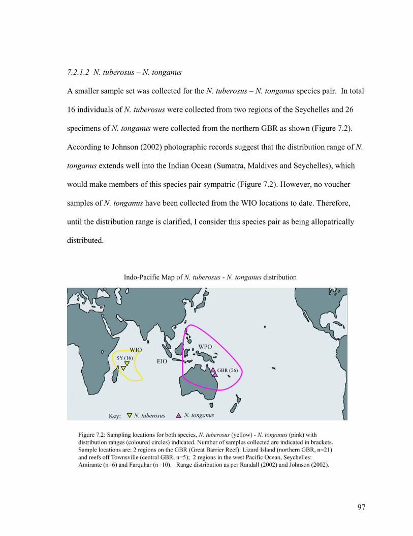
7.2.1.2 N. tuberosus – N. tonganus

A smaller sample set was collected for the N. tuberosus – N. tonganus species pair. In total

16 individuals of N. tuberosus were collected from two regions of the Seychelles and 26

specimens of N. tonganus were collected from the northern GBR as shown (Figure 7.2).

According to Johnson (2002) photographic records suggest that the distribution range of N.

tonganus extends well into the Indian Ocean (Sumatra, Maldives and Seychelles), which

would make members of this species pair sympatric (Figure 7.2). However, no voucher

samples of N. tonganus have been collected from the WIO locations to date. Therefore,

until the distribution range is clarified, I consider this species pair as being allopatrically

distributed.

98

7.2.2 Laboratory methods:

DNA extractions, PCR and direct sequencing followed protocols outlined previously in

Chapter 2.

7.2.3 Population genetic analyses

Analytical methods followed the same procedures as described in Chapter 6.

The combined species for each sister pair were analysed using a phylogenetic approach. A

ML tree (50 bootstrap replicates, outgroup-rooted with N. unicornis) was generated to

examine if the two species of a pair segregated into distinct clades and to determine if there

is geographic subdivision within species.

Population genetic analyses were used to investigate genetic differentiation, from which

levels of gene flow between populations of each species could be inferred. Pairwise Fst

comparisons were obtained for each population sampled, using AMOVA implemented in

Arlequin 2.1 (Schneider et al. 2000). To examine if any of the four species have

experienced isolation by distance (IBD), pairwise comparative Fst values of populations

were related to the pairwise geographic distances (km) between the same population pairs

(using Mantel test), using the software IBD V.1.4 (Bohonak 2002).

Haplotype (h) and percent nucleotide (π) diversities were calculated as previously

described (Chapters 5 & 6).

7.2.3.1 N. lituratus – N.elegans

The best ML topology consisting of both species pairs is illustrated.

Separate haplotype trees were generated for N. lituratus and N. elegans.

99

For this purpose, populations of N. lituratus were grouped into 5 regions: (1) WA (Western

Australia), (2) Cocos Keeling Island, (3) GBR, (4) northern PNG (Kimbe Bay, including

samples from the Solomon Islands, the Philippines and Taiwan) and (5) Hawaii (see Figure

7.1). This grouping was maintained for the analyses of AMOVA (gene flow), IBD

(isolation by distance), nucleotide - and haplotype diversity indices.

The N. elegans populations were also grouped into 5 regions for the haplotype tree and for

analyses of AMOVA, IBD and the diversity indices. Three of the 5 regions were in the

Seychelles: (1) Amirante (south of Mahe), (2) Mahe (main Island, north) and (3) Farquhar

(south of Amirante, north of Madagascar) (4) Oman and (5) Cocos Keeling Island (Figure

7.1).

7.2.3.2 N. tuberosus – N. tonganus

Likewise, the best ML tree consisting of both species pairs is presented.

A combined haplotype tree was obtained for N. tuberosus and N. tonganus due to small

sample size. The population of N. tuberosus was grouped into 2 regions in the Seychelles:

(1) Amirante (south of Mahe the main Island) and (2) Farquhar (north of Madagascar)

(Figure 7.2). The N. tonganus populations were grouped into 2 regions on the GBR: (1)

Lizard Island (northern GBR) and (2) Reefs off Townsville (central GBR) (Figure 7.2).

These groupings were maintained for both species to examine AMOVA, IBD and diversity

indices.

100

7.3 Results

7.3.1 N. lituratus – N. elegans sister species

A total of 355bp from the 3’ end of the tRNA-Pro gene and the 5’ end of the control region

were used for all analyses. The transition to transversion ratio was 2.4:1 and 3.3:1for N.

lituratus and N. elegans respectively. Of 229 or 193 polymorphic sites, 177 and 112 were

parsimony informative for N. lituratus and N. elegans respectively. The control region

(mtDNA) was A-T rich (72%) for both species as has been previously reported for fish

species (e.g. McMillan and Palumbi 1997).

The substitution model, GTR + I + Γ, was used in the ML analysis for the combined

species N. lituratus – N. elegans. A total of 71 ML trees were obtained, but only the best

tree (lnL -8279.501) was used (Figure 7.3). The rooted tree (Figure 7.3) generated two

distinct clades with high bootstrap support including individuals of both species from

Cocos Keeling. Furthermore, all individuals of the mixed sample set from Cocos Keeling

Island (n = 21), where both species co-occurred, segregated into one or other of the distinct

sister clades. Seven of the mixed-up sample set turned out to be N. elegans, and 14 grouped

into the N. lituratus clade.

Within each species clade, there was no segregation into distinct geographic regions,

despite the presence of 2 major clades for which bootstrap support however, was lacking.

Each major clade contained additional sub-clades in both species groups, indicating

substantial genetic divergence within species, though bootstrap support was again lacking

for clades (Figure 7.3).

101

102

Furthermore, there was no evidence of gene flow between the sister species N. lituratus and

N. elegans (Φst =0.75), further indication that these species are distinct and probably

reproductively isolated.

This lack of geographic structure became especially clear when examining the haplotype

trees (reduced no. of sites, 300bp see Figure 7.5 & 7.6) (N. lituratus and N. elegans

respectively). Both haplotype trees had a very limited number of shared haplotypes for the

full data set (355bp, not shown).

7.3.1.1 N. lituratus

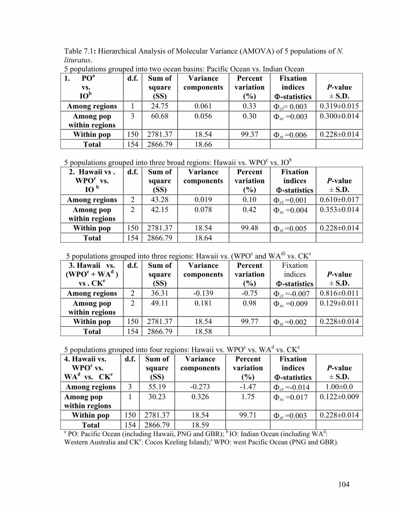
The AMOVA analysis supported the lack of geographic subdivision, evident from

inspection of the data, among regions, among populations within regions and within

populations (Table 7.1).

More than 99.4% of the observed sequence variation was within populations (Table 7.1).

Accordingly, there was almost no genetic differentiation among regions or among

populations within regions, as indicated by small, non-significant Φ-statistics (Table 7.1).

Overall, no geographic subdivision was detected and the average Φst for all regions was

0.005 with P=0.228, indicating high levels of gene flow between regions.

Comparative pairwise Fst values among the 5 populations also suggested high levels of

gene flow (Table 7.2) between all regions. Furthermore, there was no effect of isolation by

distance (either for the comparison of genetic distance: Fst and geographic distance (km) or

by log transforming both genetic and geographic distances; in both cases p>0.33). This

again supported the lack of geographic subdivision.

103

104

Table 7.1: Hierarchical Analysis of Molecular Variance (AMOVA) of 5 populations of N. lituratus. 5 populations grouped into two ocean basins: Pacific Ocean vs. Indian Ocean 1. POa vs. IOb

d.f. Sum of square

(SS)

Variance components

Percent variation

(%)

Fixation indices

Φ-statistics

P-value ± S.D.

Among regions 1 24.75 0.061 0.33 Φct= 0.003 0.319±0.015Among pop

within regions 3 60.68 0.056 0.30 Φsc =0.003 0.300±0.014

Within pop 150 2781.37 18.54 99.37 Φst =0.006 0.228±0.014Total 154 2866.79 18.66

5 populations grouped into three broad regions: Hawaii vs. WPOc vs. IOb

2. Hawaii vs . WPOc vs.

IO b

d.f. Sum of square

(SS)

Variance components

Percent variation

(%)

Fixation indices

Φ-statistics

P-value ± S.D.

Among regions 2 43.28 0.019 0.10 Φct =0.001 0.610±0.017Among pop

within regions 2 42.15 0.078 0.42 Φsc =0.004 0.353±0.014

Within pop 150 2781.37 18.54 99.48 Φst =0.005 0.228±0.014Total 154 2866.79 18.64

5 populations grouped into three regions: Hawaii vs. (WPOc and WAd) vs. CKe

3. Hawaii vs. (WPOc + WAd )

vs . CKe

d.f. Sum of square

(SS)

Variance components

Percent variation

(%)

Fixation indices

Φ-statistics

P-value ± S.D.

Among regions 2 36.31 -0.139 -0.75 Φct =-0.007 0.816±0.011Among pop

within regions 2 49.11 0.181 0.98 Φsc =0.009 0.129±0.011

Within pop 150 2781.37 18.54 99.77 Φst =0.002 0.228±0.014Total 154 2866.79 18.58

5 populations grouped into four regions: Hawaii vs. WPOc vs. WAd vs. CKe

4. Hawaii vs. WPOc vs. WAd vs. CKe

d.f. Sum of square

(SS)

Variance components

Percent variation

(%)

Fixation indices

Φ-statistics

P-value ± S.D.

Among regions 3 55.19 -0.273 -1.47 Φct =-0.014 1.00±0.0 Among pop within regions

1 30.23 0.326 1.75 Φsc =0.017 0.122±0.009

Within pop 150 2781.37 18.54 99.71 Φst =0.003 0.228±0.014Total 154 2866.79 18.59

a PO: Pacific Ocean (including Hawaii, PNG and GBR); b IO: Indian Ocean (including WAd: Western Australia and CKe: Cocos Keeling Island);c WPO: west Pacific Ocean (PNG and GBR).

105

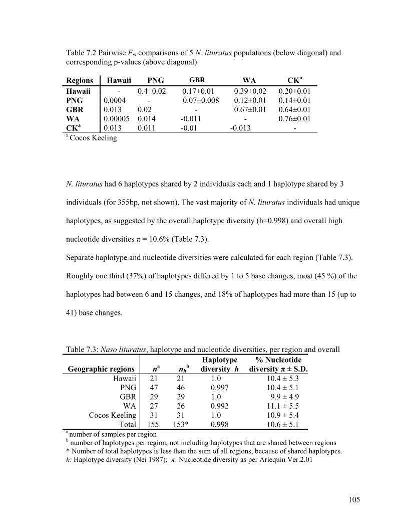
Table 7.2 Pairwise Fst comparisons of 5 N. lituratus populations (below diagonal) and corresponding p-values (above diagonal). Regions Hawaii PNG GBR WA CKa

Hawaii - 0.4±0.02 0.17±0.01 0.39±0.02 0.20±0.01 PNG 0.0004 - 0.07±0.008 0.12±0.01 0.14±0.01 GBR 0.013 0.02 - 0.67±0.01 0.64±0.01 WA 0.00005 0.014 -0.011 - 0.76±0.01 CKa 0.013 0.011 -0.01 -0.013 - a Cocos Keeling

N. lituratus had 6 haplotypes shared by 2 individuals each and 1 haplotype shared by 3

individuals (for 355bp, not shown). The vast majority of N. lituratus individuals had unique

haplotypes, as suggested by the overall haplotype diversity (h=0.998) and overall high

nucleotide diversities π = 10.6% (Table 7.3).

Separate haplotype and nucleotide diversities were calculated for each region (Table 7.3).

Roughly one third (37%) of haplotypes differed by 1 to 5 base changes, most (45 %) of the

haplotypes had between 6 and 15 changes, and 18% of haplotypes had more than 15 (up to

41) base changes.

Table 7.3: Naso lituratus, haplotype and nucleotide diversities, per region and overall

Geographic regions

na

nhb

Haplotype diversity h

% Nucleotide diversity π ± S.D.

Hawaii 21 21 1.0 10.4 ± 5.3 PNG 47 46 0.997 10.4 ± 5.1 GBR 29 29 1.0 9.9 ± 4.9 WA 27 26 0.992 11.1 ± 5.5

Cocos Keeling 31 31 1.0 10.9 ± 5.4 Total 155 153* 0.998 10.6 ± 5.1

a number of samples per region b number of haplotypes per region, not including haplotypes that are shared between regions * Number of total haplotypes is less than the sum of all regions, because of shared haplotypes. h: Haplotype diversity (Nei 1987); π: Nucleotide diversity as per Arlequin Ver.2.01

106

7.3.1.2 N. elegans

Similar results were obtained from analyses of N. elegans populations. The haplotype tree

showed a lack of population genetic structure for N. elegans (Figure 7.6). Samples from all

locations were dispersed throughout the haplotype tree.

The AMOVA results for N. elegans were similar to those for N. lituratus and again

indicated a lack of geographic subdivision. High levels of gene flow were indicated by an

average Φst for all 5 regions of -0.0007, P=0.48, and no significant difference amongst

regions, among populations within regions or within populations relative to the total

sample, was recognized (Table 7.4). Again, more than 97.6% of the observed sequence

variation was within populations (Table 7.4). Due to the limited number of samples from

Oman, they were excluded from further AMOVA analyses. The 4 regions still had a low

overall Φst (0.008, P=0.271), indicating high levels of gene flow. An exception was the

Amirante population of the Seychelles, which showed restricted gene flow among regions

(Amirante vs. Mahe, Farquhar and Cocos Keeling) p<0.05 (Table 7.4).

This was also suggested, but not significantly (Φst =0.03, P=0.09), when only the two

populations of the same sample size (Amirante vs. Cocos Keeling) were compared. It

appears that the population of Amirante is different from the other populations from the

Seychelles. However, gene flow amongst populations of the Seychelles only (Φst = 0.02,

P=0.21) was reduced, compared to levels of gene flow across the Indian Ocean (see overall

Φst values above).

107

108

Table 7.4: Hierarchical Analysis of Molecular Variance (AMOVA) of 4 populations of N. elegans. 4 populations grouped into two broad regions: WIOa vs. EIOb

1. WIOa vs. EIOb

d.f. Sum of square

(SS)

Variance components

Percent variation

(%)

Fixation indices

Φ-statistics

P-value ± S.D.

Among regions 1 19.70 -0.116 -0.62 Φct =-0.006 0.251±0.015Among pop

within regions 2 43.22 0.222 1.18 Φsc =0.012 0.215±0.011

Within pop 62 1153.97 18.61 99.44 Φst =0.006 0.271±0.016Total 65 1216.88 18.72

4 populations grouped into two regions: Amirante (Seychelles) vs. remaining 2 sites of Seychelles and Cocos Keeling Island

2. Amirante vs. rest

d.f. Sum of square

(SS)

Variance components

Percent variation

(%)

Fixation indices

Φ-statistics

P-value ± S.D.

Among regions 1 35.24 0.81 4.25 Φct =0.04 0.00±0.00* Among pop

within regions 2 27.67 -0.35 -1.85 Φsc =-0.02 0.815±0.01

Within pop 62 1153.97 18.61 97.60 Φst =0.02 0.271±0.016Total 65 1216.88 19.07

a WIO: West Indian Ocean: 3 regions of Seychelles: Mahe, Amirante and Farquhar b EIO: East Indian Ocean (Cocos Keeling Island) * p≤0.05, significantly different

The pairwise Fst comparisons among all 5 populations produced no significant differences

(p<0.05) between haplotypes (Table 7.5). However, it appears that pairwise Fst values

between Amirante - Farquhar and Amirante - Cocos Keeling were marginally higher,

indicating somewhat reduced gene flow, compared to the remaining populations, which

demonstrated high levels of gene flow.

This however, was not an effect due to isolation by distance, because the Mantel test

produced no significant difference, either when using the untransformed pairwise Fst

comparison of populations to the pairwise geographic distances (km), nor by log

transforming both matrices (p>0.7, data not shown).

109

Table 7.5: Pairwise Fst comparisons for 5 N. elegans populations (below diagonal) and corresponding p-values ± S.D. (above diagonal). Regions Oman Amirante Farquhar Mahe CKa

Oman - 0.31±0.011 0.68±0.014 0.87±0.01 0.97±0.006 Amirante 0.006 - 0.1 ±0.01 0.28±0.01 0.09±0.010 Farquhar -0.07 0.04 - 0.66±0.01 0.62±0.013 Mahe -0.08 0.01 -0.03 - 0.83±0.012 CKa -0.07 0.03 -0.01 -0.03 - a CK: Cocos Keeling

In N. elegans, only 2 haplotypes were each shared by 2 individuals (for the full data set,

355bp, not shown). All remaining haplotypes were unique (h = 0.999) and the overall

nucleotide diversity was also very high (10.4%) (Table 7.6). Again, as with N. lituratus,

there is high genetic diversity due to many base changes between haplotypes; 32% of

haplotypes differed by 1 to 5 base changes and 45% differed by 6 to 15 changes amongst

haplotypes. The remaining 23% had more than 16 (up to 46) substitutions.

Table 7.6: Naso elegans, haplotype and nucleotide diversity indices, per region and for the overall sample Geographic regions

na

nh

b Haplotype diversity h

% Nucleotide diversity π ± S.D.

Seychelles, Mahe 8 8 1.0 11.6 ± 6.4 Seychelles, Amirante 22 21 1.0 9.4 ± 4.8 Seychelles, Farquhar 14 14 1.0 10.1 ± 5.2

Oman 5 4 0.9 9.0 ± 5.6 Cocos Keeling 22 21 0.996 11.4 ± 5.8

Total 71 69 0.999 10.4 ± 5.1 a number of samples per region, b number of haplotypes per region, h: Haplotype diversity as per Nei (1987), π: Nucleotide diversity as per Arlequin Ver.2.001.

110

7.3.2 N. tuberosus – N. tonganus sister species

For all analyses 332bp of the control region were used. N. tuberosus had 77 polymorphic

sites, of which 53 were parsimony-informative. There was a transition to transversion ratio

of 3.5:1. N. tonganus had 90 polymorphic sites with 31 being parsimony-informative, and a

transition to transversion ratio of 2.5:1. The d-loop region was A-T rich (71%) for both

species as has been reported previously in this study and for other fish species (e.g.

McMillan and Palumbi 1997).

The TVM + Γ (no invariable sites) substitution model was used in the ML analysis, for the

combined species N. tuberosus – N. tonganus. In total, 44 trees were obtained, but only the

best tree (lnL -2358.52) was used (Figure 7.7). The rooted tree contained two distinct

clades with high bootstrap support. Within each clade however, no segregation of the

samples by locality was observed, a result that was also supported by the haplotype tree

(Figure 7.8).

There was no evidence of gene flow between the species (Fst 0.71).

AMOVA analyses also produced results indicating high levels of gene flow amongst

locations and within locations (Table 7.7). All of the variation (100%) was within

populations relative to the total sample.

The pairwise Fst comparisons between the two species populations produced the same

result as the Φst values in the AMOVA (Table 7.7) indicating extensive gene flow among

locations within regions.

111

112

113

Table 7.7: Hierarchical Analysis of Molecular Variance (AMOVA) of 2 populations each for N. tuberosus (A) and N. tonganus (B). Two locations for N. tuberosus: Amirante vs. Farquhar (Seychelles) A) Amirante

vs. Farquhar

d.f. Sum of square

(SS)

Variance components

Percent variation

(%)

Fixation index

Φ-statistics

P-value ± S.D.

Among regions 1 8.22 -0.05 -0.65 Within pop 14 120.97 8.64 100.65 Φst =-0.006 0.507±0.014

Total 15 106.94 8.58

Two locations for N. tonganus: Lizard Island vs. Townsville B) Lizard Island vs. Townsville

d.f. Sum of square

(SS)

Variance components

Percent variation

(%)

Fixation index

Φ-statistics

P-value ± S.D.

Among regions 1 8.11 -0.22 -2.28 Within pop 24 237.51 9.90 102.28 Φst =-0.023 0.602±0.015

Total 25 245.62 9.67 All individuals had unique haplotypes (h = 1.0), but the nucleotide diversities were slightly

lower (Table 7.8) than was obtained for N. lituratus and N. elegans. The lower nucleotide

diversities for N. tuberosus and N. tonganus may be an artefact of the reduced number of

locations and individuals sampled per species compared to N. lituratus – N. elegans and N.

vlamingii.

Table 7.8: N. tuberosus – N. tonganus, haplotype and nucleotide diversities, per location and overall

Geographic regions

na

nh

b Haplotype diversity h

% Nucleotide diversity π ± S.D.

N. tuberosus Seychelles, Amirante

6

6

1.00

4.2 ± 2.6

Seychelles, Farquhar 10 10 1.00 5.8 ± 3.2 Total 16 16 1.00 5.3 ± 2.8

N. tonganus GBR, Lizard Island

21

21

1.00

6.4 ± 3.3

GBR, off Townsville 5 5 1.00 4.5 ± 2.9 Total 26 26 1.00 6.0 ± 3.1

a number of samples per region, b number of haplotypes, h: Haplotype diversity as per Nei (1987), π: Nucleotide diversity as per Arlequin Ver.2.001

A comparison of diversity indices and Φst values for all Naso species examined in this

thesis is listed in Table 7.9.

Table 7.9: Comparative haplotype (h) and percent nucleotide (π) diversities, and Φst (as a measure of gene flow) for d-loop of this study. Species n nh Region h % π Φst Source Naso vlamingii 25 25 GBR 1.0 13.9 This study 14 14 PNG 1.0 15.1 (Chapter 6) 10 10 Philippines 1.0 14.1 7 7 WA 1.0 14.7 21 21 Seychelles 1.0 13.9 Among Oceans 0.008 WIO vs rest 0.020 77 77 All regions 1.0 14.2 0.005 Naso lituratus 47 46 PNG 0.997 10.4 This study 29 29 GBR 1.0 9.9 (Chapter 7) 27 26 WA 0.992 11.1 31 31 Cocos Keeling Island 1.0 10.9 21 21 Hawaii 1.0 10.4 Among Oceans 0.006 Hawaii vs (WPOa+WA) vs CKb 0.002 155 153 All regions 0.998 10.6 0.005 Naso elegans 44 44 Seychelles 1.0 9.4-11.6 5 4 Oman 0.9 9.0 22 21 Cocos Keeling Isl. 0.996 11.4 Amirante vs rest (excl. Oman) 0.02 WIOc (excl. Oman) vs EIOd 0.006 71 68 All regions 0.999 10.4 -0.001 Naso tuberosus 6 6 Amirante, Seychelles 1.0 4.2 10 10 Farquhar, Seychelles 1.0 5.8 16 16 Seychelles 1.0 5.3 -0.006 Naso tonganus 21 21 Lizard Isl., northern GBR 1.0 6.4 5 5 Townsville, central GBR 1.0 4.5 GBR 1.0 6.0 -0.02 a WPO: west pacific Ocean (including PNG + GBR) b CK: Cocos Keeling Isl. c WIO: west Indian Ocean (Seychelles) d EIO: east Indian Ocean (Cocos Keeling Isl.)

114

115

7.4 Discussion

This chapter demonstrated that both pairs of sister species had comparable population

structures. High connectivity was apparent for each species, due to weak/absent genetic

differentiation among populations sampled. This was also shown for N. vlamingii (chapter

6). Although, each species segregated into a distinct clade, there was a total lack of

geographic structure within each species.

Fixation indices were low, hence gene flow was higher in all Naso species relative to other

reef fish species (see also Table 5.1 in chapter 5). Naso species seem to represent one

extreme (high levels of gene flow) on a scale of reef fish population connectivity.

All 4 species investigated in this chapter displayed high haplotype and nucleotide

diversities as well as weak/no genetic differentiation (hence high levels of gene flow)

among populations sampled. The species pairs best fit category I of Avise (2000)

suggesting deep divergences of allopatric lineages. However, each species individually is

best described by Avise’s (2000) category II. The long, unstable evolutionary histories

would support the deep divergences (similar to N. vlamingii), where isolated populations

(during periods of low sea level) came into secondary contact at times of elevated sea levels

due to gene flow.

Both species pairs arose during the late Miocene (approx. between 7 – 5MY, chapter 4),

which was a time of repeated extreme oscillations in sea level (up to 50m below present

sea-level), glaciations and fluctuating sea temperatures (Hallam 1984; Haq et al. 1987;

Zachos et al. 2001a).

116

When comparing all 5 Naso species examined in the phylogeographic part of this study, N.

vlamingii (which diverged ~ 18 MYA) had the highest nucleotide diversities (13.9 to

15.1%) of all Naso species investigated. This was also true when compared to other reef

fish species studied for the same gene region (Bernardi 2000; Terry et al. 2000; Bernardi et

al. 2001; Stepien et al. 2001; Bernardi et al. 2002; Ovenden et al. 2002; Bay et al. online)

(see Table 5.1).

Both N. lituratus and N. elegans also had high nucleotide diversities in all regions (ranging

between 9.4% and 11.4%). Naso tuberosus and N. tonganus also had high nucleotide

diversities compared to other taxa, but these were the lowest of all the Naso species

investigated (4.2 to 6.4%). These lower values may be an artefact of relatively small sample

sizes compared to the other species studied or they may be real differences in substitution

rates. Additional sampling is required to resolve this issue.

To date, there is no record of a study examining surgeonfish (acanthurid) population

structure using the control region. However, Rocha et al. (2002) have used another mtDNA

marker (cyt b) for three Acanthurus species in the tropical Atlantic Ocean. These species

also had high haplotype diversities (h=0.7 – 0.94), but they had low nucleotide diversities

(π= 0.0 – 0.6%). The 3 Acanthurus species had an average PLD (planktonic larval

duration) of 52 days (Rocha et al. 2002). Two of the three species demonstrated strong (Φst

0.72, A. bahianus) to moderate (Φst 0.36, A. coeruleus) population genetic structure, whilst

the third species (A. chirurgus) had high levels of gene flow (Φst 0.002- 0.05) and lacked

population genetic structure, even across the plume of the Amazon Basin. The authors

attributed this lack of genetic segregation to the ability of A. chirurgus to tolerate low

117

salinity levels at the muddy bottom of the Atlantic Ocean when they cross the Amazon

barrier, which often forms a biogeographic barrier to species (Rocha et al. 2002). Although

these diversity indices are for cyt b, two separate studies have demonstrated that nucleotide

diversities for sequence data from cyt b are between 5 and 7 times lower than nucleotide

diversities obtained from sequence data of the control region (Bowen and Grant 1997;

Grant and Bowen 1998; Bernardi et al. 2001). In the first of these studies, Bowen & Grant

(1997) examined both cyt b and d-loop sequence data for the same temperate marine

species of sardines (Sardinops) from 5 regions worldwide. Nucleotide diversities for d-loop

were on average 4.3 times as high as those obtained from cyt b. In the second of these

studies, Bernardi et al. (2001) reported an average rate that was 5.8 times as fast for d-loop

than for cyt b in the damselfish D. trimaculatus. If nucleotide diversities obtained from cyt

b sequences are “corrected” by a factor of between 5 and 7, it is possible to compare

nucleotide diversities (π) between these markers. If such a “correction” is applied to the cyt

b nucleotide diversities of the Acanthurus species of Rocha et al (2002), then the nucleotide

diversity would range from 0.0-3.6%. Even these nucleotide diversity values for

Acanthurus species are low compared to nucleotide diversities of Naso species in this

study, which ranged from 4.2 to 15.1%. This is true, despite the fact that they are from the

same family and display similar life history traits, such as extended dispersal abilities,

relatively short generation times (compared to their longevity) and extended life spans, all

of which increase genetic homogeneity by reducing genetic differentiation among

populations. Acanthurus species are probably more recent than Naso species (Clements et

al. 2003, phylogeny and timing of divergence this study), which may explain the observed

reduced nucleotide diversity.

118

It appears that an allopatric mode of speciation operated for both species pairs (N. lituratus

– N. elegans and N. tuberosus – N. tonganus) studied here, because sister taxa in each

species pair occur in different ocean basins. Species have presumably diverged while

geographically isolated. Even if they do co-occur, as is the case with N. lituratus – N.

elegans in Cocos Keeling, probably due to range expansion, they are readily

distinguishable as separate species based on colour patterns (Randall 2002). This

distinctiveness of both species pairs was also supported by molecular phylogenetic analysis

of the genus (chapter 3). They appear to be reproductively isolated, as they are genetically

distinct in sympatry. The extreme conditions of the Miocene must have isolated ancestral

lineages of the four examined Naso species for sufficient periods of time to achieve

reproductive isolation in allopatry. The time since divergence of these two species pairs (N.

lituratus – N. elegans ~ 5.2MY and N. tuberosus – N. tonganus ~ 6.6MY) suggests an

unstable evolutionary history as was found for N. vlamingii. Tectonic events (continental

drift) and subsequent geographic isolation at times of reduced sea level most likely drove

the speciation.

This stands in strong contrast to the lack of speciation (even cryptic) observed for N.

vlamingii (Chapter 6). Why is it then that the sister taxa N. lituratus – N. elegans speciated

in allopatry (over “short” evolutionary time, approx. 6MY) but N. vlamingii did not over a

much longer evolutionary period (approx. 18MY)?

Certain traits may have contributed to differences effecting the speciation process between

N. lituratus – N. elegans and N. vlamingii. Despite the fact that all Naso species share an

extensive dispersal capability as larvae, two traits, dietary and habitat use as adults may

have contributed to the difference. Naso vlamingii, a generalist with a semi-pelagic habitat

119

use, is probably better equipped to utilise different habitats (e.g. deeper and offshore

movements/migrations) and food sources (omnivore), therefore may also be better able to

adjust/adapt to changing conditions compared to the sister taxa. Whereas the sister taxa, N.

lituratus – N. elegans, are more restricted by their dietary habit (feeding exclusively on

algae) and need to live and stay close to coral reefs. This restriction may also affect the

ability of dispersive larvae to persist to maturity when settling to different habitats. Further

sampling of individuals from e.g. the central Pacific Ocean may help to elucidate this point.

In summary, all species had weak genetic differentiation (high levels of gene flow) among

populations across their distribution range and high diversity indices. This suggests that all

species have had a lengthy, unstable evolutionary history with repeated (at low sea levels)

cycles of isolation and lineage divergence, followed by re-mixing (secondary contact) at

times of elevated sea levels.

This study confirms that putative sister species of Naso examined here are reproductively

isolated (no gene flow), despite the extensive dispersal capabilities of their larvae. Even

when they co-occur (N. lituratus and N. elegans in Cocos Keeling), they do not interbreed

or hybridise. Given their allopatric distributions, it is likely that speciation occurred in

allopatry at times of low sea level stand.