International Journal of Mathematics Trends and Technology-Volume 19 number 1. March 2015

Comparative Study of Bisection andNewton-Rhapson Methods of

Root-Finding Problems

ABDULAZIZ G. AHMADagarbaahmad@yahoo.com

Department of Mathematics

National Mathematical Center Abuja, Nigeria

Abstract-This paper presents two numerical techniques of root-finding problems of a non-linear equations with the assumption that a solution exists, the rate of convergence of Bisectionmethod and Newton-Rhapson method of root-finding is also been discussed. The software pack-age, MATLAB 7.6 was used to find the root of the function, f(x) = cosx−x∗exp(x) on a closeinterval [0, 1] using the Bisection method and Newton’s method the result was compared. Itwas observed that the Bisection method converges at the 14th iteration while Newton methodsconverge to the exact root of 0.5718 with error 0.0000 at the 2nd iteration respectively. It wasthen concluded that of the two methods considered, Newton’s method is the most effectivescheme. This is in line with the result in our Ref.[9].

Keywords:-Convergence, Roots, Algorithm, MATLAB Code, Iterations, Bisection method,Newton-Rhapson method and function

1 INTRODUCTION

An expression of the form f(x) = a0xn + a1x

n−1 + ... + an−1 + an, where a′s are costants(a0 6= 0) and n is a positive integer, is called a polynomial of degree n in x. if f(x) containssome other functions as trigonometric, logarithmic, exponential etc. then, f(x) = 0 is calleda transcendental equation. The value of α of x which satisfies f(x) = 0 is called a root off(x) = 0, and a process to find out a root is known as root finding. Geometrically, a root isthat value of (x) where the graph of y = f(x) crosses the x-axis.The root finding problem is one of the most relevant computational problems. It arises ina wide variety of practical applications in Sciences and Engineering. As a matter of fact,the determination of any unknown appearing implicitly in scientific or engineering formulas,gives rise to root finding problem [1]. Relevant situations in Physics where such problems areneeded to be solved include finding the equilibrium position of an object, potential surface ofa field and quantized energy level of confined structure [2]. The common root-finding methodsinclude: Bisection and Newton-Rhapson methods etc. Different methods converge to the rootat different rates. That is, some methods are faster in converging to the root than others. Therate of convergence could be linear, quadratic or otherwise. The higher the order, the fasterthe method converges [3]. The study is at comparing the rate of performance (convergence) ofBisection and Newton-Rhapson as methods of root-finding.Obviously, Newton-Rhapson method may converge faster than any other method but when

ISSN: 2231-5373 http://www.ijmttjournal.org page 1

International Journal of Mathematics Trends and Technology-Volume 19 number 1. March 2015

we compare performance, it is needful to consider both cost and speed of convergence. Analgorithm that converges quickly but takes a few seconds per iteration may take more timeoverall than an algorithm that converges more slowly, but takes only a few milliseconds periteration [5].In comparing the rate of convergence of Bisection and Newton’s Rhapson methods[8] used MATLAB programming language to calculate the cube roots of numbers from 1 to25, using the three methods. They observed that the rate of convergence is in the followingorder: Bisection method < Newton’s Rhapson method. They concluded that Newton methodis 7.678622465 times better than the Bisection method.

2 BISECTION METHOD

The Bisection Method [1] is the most primitive method for finding real roots of function f(x) = 0where f is a continuous function. This method is also known as Binary-Search Method andBolzano Method. Two initial guess is required to start the procedure. This method is basedon the Intermediate value theorem:Let function f(x) = 0 be continuous between a and b. For definiteness, let f(a) and f(b) haveopposite signs and less than zero. Then the first approximations to the root is x1 = 1

2(a+ b). if

f(x1) = 0 otherwise, the root lies between a and x1 0r x1 and b according as f(x1) is positiveor negative. Then we Bisect the interval as before and continue the process until the root isfound to the desired accuracy.

Algorithm of Bisection Method for root-findingInput:

i f(x) is the given function

ii a, b the two numbers such that f(a)f(b) < 0

Output:An approximatin of the root of f(x) = 0 in [a, b], for k = 0, 1, 2, 3... do untill satisfied.

i ck = ak+bk2

ii Test if ck is desired root. if so, stop.

iii If ck is not the desired root, test if f(ck)f(ak) < 0. if so, set bk + 1 = ck and ak + 1 = ck.otherwise ck = bk + 1 = bk

End

Stopping Criteria for Bisection MethodThe stopping criteria as suggested by [5]: that let e be the error tolerance, that is we wouldlike to obtain the root with an error of at most of e. Then, accept x = ck as root of f(x) = 0.if any of the following criteria satisfied

1 |f(ck)|≤e (i.e the functional value is less than or equal to the tolerance).

ii | ck−1−ckck|≤e (i.e the relative change is less than or equal to the tolerance).

iii b−a2k|≤e (i.e the length of the interval after k iterations is less than or equal to tolerance).

ISSN: 2231-5373 http://www.ijmttjournal.org page 2

International Journal of Mathematics Trends and Technology-Volume 19 number 1. March 2015

iv The number of iterations k is greater than or equal to a predetermined number, say N .

Theorem 1: The number of iterations, N needed in the Bisection method to obtain an accu-racy of is given by: N≥ log(b−a)−log(e)

log2

Proof :Let the interval length after N iteration be b−a2N

. So to obtain an accuracy of b−a2N≤e.

That is → −Nlog2≤log( eb−a) → Nlog( e

b−a) N≥−log(e

b−a)

log2Therefore N≥ log(b−a)−log(e)

log2

Note: Since the number of iterations, N needed to achieve a certain accuracy depends uponthe initial length of the interval containing the root, it is desirable to choose the initial interval[a, b] as small as possible.

MATLAB code of Bisection Method

function root = bisection23(fname,a,b,delta,display)

% The bisection method.

%

%input: fname is a string that names the function f(x)

% a and b define an interval [a,b]

% delta is the tolerance

% display = 1 if step-by-step display is desired,

% = 0 otherwise

%output: root is the computed root of f(x)=0

%

fa = feval(fname,a);

fb = feval(fname,b);

if sign(fa)*sign(fb) > 0

disp(’function has the same sign at a and b’)

return

end

if fa == 0,

root = a;

return

end

if fb == 0

root = b;

return

end

c = (a+b)/2;

fc = feval(fname,c);

e_bound = abs(b-a)/2;

if display,

disp(’ ’);

disp(’ a b c f(c) error_bound’);

disp(’ ’);

disp([a b c fc e_bound])

end

while e_bound > delta

if fc == 0,

ISSN: 2231-5373 http://www.ijmttjournal.org page 3

International Journal of Mathematics Trends and Technology-Volume 19 number 1. March 2015

root = c;

return

end

if sign(fa)*sign(fc) < 0 % a root exists in [a,c].

b = c;

fb=fc;

else % a root exists in [c,b].

a = c;

fa = fc;

end

c = (a+b)/2;

fc = feval(fname,c);

e_bound = e_bound/2;

if display, disp([a b c fc e_bound]), end

end

root = c;

Example: I solve f(x) = cosx − xexp(x) = 0 at [0, 1] using Bisection method with aid ofthe MATLAB Code.

Solution: Input from the MATLAB command window.

>> fname = @(x)(cos(x)-x*exp(x));

>> a=0;

>> b=1;

>> display=1;

>> delta=10^-4;

>> root = bisection23(fname,a,b,delta,display)

Table 1

n a b c f(c) error_bound

1 0 1.0000 0.5000 0.0532 0.5000

2 0.5000 1.0000 0.7500 -0.8561 0.2500

3 0.5000 0.7500 0.6250 -0.3567 0.1250

4 0.5000 0.6250 0.5625 -0.1413 0.0625

5 0.5000 0.5625 0.5313 -0.0415 0.0313

6 0.5000 0.5313 0.5156 0.0065 0.0156

7 0.5156 0.5313 0.5234 -0.0174 0.0078

8 0.5156 0.5234 0.5195 -0.0054 0.0039

ISSN: 2231-5373 http://www.ijmttjournal.org page 4

International Journal of Mathematics Trends and Technology-Volume 19 number 1. March 2015

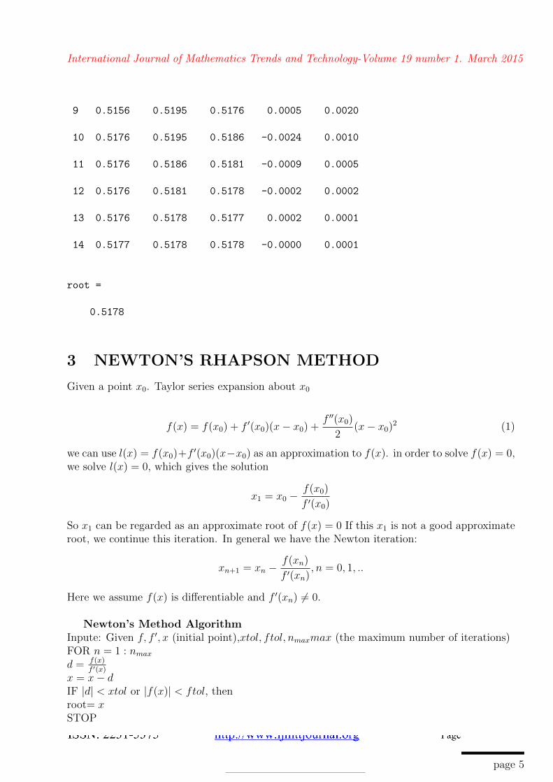
9 0.5156 0.5195 0.5176 0.0005 0.0020

10 0.5176 0.5195 0.5186 -0.0024 0.0010

11 0.5176 0.5186 0.5181 -0.0009 0.0005

12 0.5176 0.5181 0.5178 -0.0002 0.0002

13 0.5176 0.5178 0.5177 0.0002 0.0001

14 0.5177 0.5178 0.5178 -0.0000 0.0001

root =

0.5178

3 NEWTON’S RHAPSON METHOD

Given a point x0. Taylor series expansion about x0

f(x) = f(x0) + f ′(x0)(x− x0) +f ′′(x0)

2(x− x0)2 (1)

we can use l(x) = f(x0)+f ′(x0)(x−x0) as an approximation to f(x). in order to solve f(x) = 0,we solve l(x) = 0, which gives the solution

x1 = x0 −f(x0)

f ′(x0)

So x1 can be regarded as an approximate root of f(x) = 0 If this x1 is not a good approximateroot, we continue this iteration. In general we have the Newton iteration:

xn+1 = xn −f(xn)

f ′(xn), n = 0, 1, ..

Here we assume f(x) is differentiable and f ′(xn) 6= 0.

Newton’s Method AlgorithmInpute: Given f, f ′, x (initial point),xtol, ftol, nmaxmax (the maximum number of iterations)FOR n = 1 : nmax

d = f(x)f ′(x)

x = x− dIF |d| < xtol or |f(x)| < ftol, thenroot= xSTOP

ISSN: 2231-5373 http://www.ijmttjournal.org page 5

International Journal of Mathematics Trends and Technology-Volume 19 number 1. March 2015

ENDENDroot= xStopping criteria

1. |xn+1 − xn| < xtol

2. |f(xn+1)| < ftol

3. the maximum number of criteria reached

Failure of Newton’s Rhapson Method Newton’s method does not always works well.It may not converge.

• If f ′(xn) = 0 the method is not defined.

• If f ′(xn) approximate to 0 then there may be difficulties. The new estimate xn + 1 maybe a much worse approximation to the solution than xn is.

Convergence Analysis of Newton’s Method Def. Quadratic convergence (QC). Asequence xn is said to have QC to a limit x if

limn=∞

|xn+1 − x||xn − x|2

= c, (2)

where c is some finite non-zero constant.Newton iteration:

xn+1 = xn −f(xn)

f ′(xn)(3)

Suppose xn converges to a root r of f(x) = 0. Taylor series expansion about xn is

f(r) = f(xn) + f ′(xn)(r − xn) +f ′′(zn)

2(r − xn)2 (4)

where zn lies between xn and r.But f(r) = 0, and dividing by f ′(xn)

0 =f(xn)

f ′(xn)+ (r − xn) +

f ′′(zn)

2f ′(xn)(r − xn)2

The first term on the RHS is xn − xn+1, so

r − xn+1 = cn(r − xn)2, cn = f ′′(zn)2f ′(xn)

Writing the error en = r − xn, we see

en+1 = cn(en)2

Since xn approached r, and zn is between xn and r, we see zn appraoched r and so

limn=∞

|en+1||en|2

= limn=infty

|cn| =f ′′(r)

2f ′(r)= cn,

ISSN: 2231-5373 http://www.ijmttjournal.org page 6

International Journal of Mathematics Trends and Technology-Volume 19 number 1. March 2015

assuming that f ′(r) 6= 0.So the convergence rate of Newton method is usually quadratical. At the (n + 1)th step, thenew error is equal to cn times the square of the old error. Also we can show f(xn) usuallyconverges to 0 quadratically.

MATLAB code of Newton’s Rhapson

function root=newton24(fname,fdname,x,xtol,ftol,n_max,display)

% Newton’s method.

%

%input:

% fname string that names the function f(x).

% fdname string that names the derivative f’(x).

% x the initial point

% xtol and ftol termination tolerances

% n_max the maximum number of iteration

% display = 1 if step-by-step display is desired,

% = 0 otherwise

%output: root is the computed root of f(x)=0

%

n = 0;

fx = feval(fname,x);

if display,

disp(’ n x f(x)’)

disp(’-------------------------------------’)

disp(sprintf(’%4d %23.4e %23.4e’, n, x, fx))

end

if abs(fx) <= xtol

root = x;

return

end

for n = 1:n_max

fdx = feval(fdname,x);

d = fx/fdx;

x = x - d;

fx = feval(fname,x);

if display,

disp(sprintf(’%4d %23.4e %23.4e’,n,x,fx))

end

if abs(d) <= xtol | abs(fx) <= ftol

root = x;

return

end

end

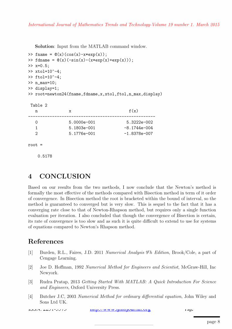
Example: I solve f(x) = x− cosx = 0 at [0, 1] using Newton Rhapson method with aid ofthe MATLAB Code.

ISSN: 2231-5373 http://www.ijmttjournal.org page 7

International Journal of Mathematics Trends and Technology-Volume 19 number 1. March 2015

Solution: Input from the MATLAB command window.

>> fname = @(x)(cos(x)-x*exp(x));

>> fdname = @(x)(-sin(x)-(x*exp(x)+exp(x)));

>> x=0.5;

>> xtol=10^-4;

>> ftol=10^-4;

>> n_max=10;

>> display=1;

>> root=newton24(fname,fdname,x,xtol,ftol,n_max,display)

Table 2

n x f(x)

-----------------------------------------------------

0 5.0000e-001 5.3222e-002

1 5.1803e-001 -8.1744e-004

2 5.1776e-001 -1.8378e-007

root =

0.5178

4 CONCLUSION

Based on our results from the two methods, I now conclude that the Newton’s method isformally the most effective of the methods compared with Bisection method in term of it orderof convergence. In Bisection method the root is bracketed within the bound of interval, so themethod is guaranteed to converged but is very slow. This is sequel to the fact that it has aconverging rate close to that of Newton-Rhapson method, but requires only a single functionevaluation per iteration. I also concluded that though the convergence of Bisection is certain,its rate of convergence is too slow and as such it is quite difficult to extend to use for systemsof equations compared to Newton’s Rhapson method.

References

[1] Burden, R.L., Faires, J.D. 2011 Numerical Analysis 9th Edition, Brook/Cole, a part ofCengage Learning.

[2] Joe D. Hoffman, 1992 Numerical Method for Engineers and Scientist, McGraw-Hill, IncNewyork.

[3] Rudra Pratap, 2013 Getting Started With MATLAB: A Quick Introduction For Scienceand Engineers, Oxford University Press.

[4] Butcher J.C, 2003 Numerical Method for ordinary differential equation, John Wiley andSons Ltd UK.

ISSN: 2231-5373 http://www.ijmttjournal.org page 8

International Journal of Mathematics Trends and Technology-Volume 19 number 1. March 2015

[5] Kendalle E. Atkinson, 2004 An Introduction To Numerical Analysis, John Wiley and SonsLtd UK.

[6] Radhey S. Gupta, 2009 Element of Numerical Analysis, Macmillan India Ltd.

[7] Chadha, N.M, 2014 Lecture Note On MATLAB, Sharda University.

[8] Cleve B. Moler, Numerical Computing With MATLAB, PHI Leraning, Rimjhim houseDelhi, 2013.

[9] Noreen, Jamil, A Comparison of Iterative Methods for the Solution of Non-Linear Systemsof equations,Int. J. Emerg. Sci., 3(2), 119-130, June 2013

ISSN: 2231-5373 http://www.ijmttjournal.org page 9