62
Prepared by: Kiwa GASTEC at CRE Prepared for: Warwick University Contract Number: 30197 Date: March 2014 Comparative testing of a gas absorption heat pump on the dynamic test rig
| Date post: | 16-Sep-2018 |
| Category: |
Documents |
| Upload: | truongngoc |
| View: | 224 times |
| Download: | 0 times |

Prepared by: Kiwa GASTEC at CRE Prepared for: Warwick University Contract Number: 30197 Date: March 2014
Comparative testing of a gas
absorption heat pump on the
dynamic test rig
Warwick University 30197
© Kiwa Ltd 2014
Comparative testing of a gas absorption heat pump on the
dynamic test rig
Prepared by
Name Helen Charlick
Position Energy Consultant
Name Mark Crowther
Position Director and General Manager
Name Tim Dennish
Position Principal Consultant
Name James Thomas
Position Energy Consultant
Approved by
Name Iain Summerfield
Position Principal Consultant
Date March 2014
Commercial in Confidence
Kiwa GASTEC at CRE Kiwa Ltd The Orchard Business Centre Stoke Orchard Cheltenham GL52 7RZ UK Telephone: +44 (0)1242 677877 Fax: +44 (0)1242 676506 E-mail: [email protected] Web: www.kiwa.co.uk

Warwick University 30197
© Kiwa Ltd 2014
Executive Summary
The performance of gas absorption heat pumps has been compared to the more
established technologies of air source heat pumps and conventional condensing boilers for
the purposes of space heating.
This test programme used Kiwa’s unique Dynamic Heat Load Test Rig. This rig combines
testing of real hardware in a software simulation loop, which provides realistic and
reproducible heating loads over a period of 24 hours, allowing different heating
technologies to easily be compared.
Three technologies were compared – a gas absorption heat pump (GAHP), an electric air
source heat pump (ASHP) and a combination condensing gas boiler. Two simulated
houses were used as the test basis: one with average UK heat demand and one with a
substantial heat demand, representing a very large property.
The results indicate that the daily energy consumption of a property strongly depends upon:
The ability of the system to operate bimodally or unimodally whilst giving acceptable
internal temperatures. This is a function of appliance operating temperature, and kW
output rating at this temperature.
o Bimodal – heating pattern where the heating appliance is enabled twice a
day: between 07:00 to 09:00 and 16:00 to 23:00. This is as per SAP and is
used in the dynamic test rig program.
o Unimodal – heating appliance is enabled for one period a day from 07:00 -
23:00.
o Continuous – heating appliance is enabled for 24 hours a day.
External temperature
System water temperature (especially return)
The instantaneous and average efficiency of the appliance
Primary fuel use (assuming electricity is supplied from a combined cycle gas turbine* with
an efficiency of 47.7%1) is a strong function of both electric and gas usage of the device,
not just the gas.
Beyond this the work demonstrates the sheer complexity of trying to compare the heat
required, the gas plus electricity used and primary energy equivalence of both small and
large houses. Different heating patterns with different appliances and different heat emitter
temperatures will markedly affect both the reported efficiency and the actual energy used. A
somewhat higher efficiency for the appliance may not save primary energy, if the
technology used to obtain the high efficiency results in the building remaining at a higher
average temperature and thus using more primary energy.
The following tables compare total carbon emissions to maintain a property at the declared
average internal temperatures (shown in brackets) when the external temperatures are 0⁰C

Warwick University 30197
© Kiwa Ltd 2014
and 7⁰C . For comparison UK field trials show average internal temperatures in the range
17.7⁰C 2.
Daily carbon emissions (kgCO2e/day)
(Average internal temperature (°C))
Small house (300W/K) Large house (700W/K)
External temp 0⁰C Boiler ASHP Boiler GAHP
Bimodal Rads 60⁰C N/T N/T N/T N/T
Bimodal Rads 45⁰C N/T N/T N/T N/T
Unimodal Rads 60⁰C 27.5 (19.0)
29.0 (17.7)
61.7 (18.5)
60.6 (18.4)
Unimodal Rads 45⁰C 26.9 (18.9)
N/T N/T N/T
Continuous Rads 60⁰C N/T 34.2 (20.8)
N/T N/T
Continuous Rads 45⁰C 30.5 (20.9)
30.5 (20.8)
65.0 (20.9)
63.1 (20.8)
External temp 7⁰C Boiler ASHP Boiler GAHP
Bimodal Rads 60⁰C 17.9 (18.8)
N/T 37.5 (18.2)
37.1 (18.2)
Bimodal Rads 45⁰C N/T N/T N/T N/T
Unimodal Rads 60⁰C 20.0 (20.3)
17.4 (19.5)
N/T N/T
Unimodal Rads 45⁰C 19.4 (20.0)
N/T 42.4 (19.8)
40.2 (19.8)
Continuous Rads 60⁰C N/T 19.3 (20.9)
N/T N/T
Continuous Rads 45⁰C N/T 16.4 (20.9)
N/T N/T
Key: N/T = Not tested as would not be realistic of operation of the appliance in the field.
Reasons for this may include: there would be insufficient heat output from the appliance to meet the heat
demand of the house, the radiators would be too small to deliver sufficient energy to the house, or the
appliance would cycle too frequently.
The equivalent CO2 emissions were calculated, assuming emissions factors of
0.5173 kgCO2e/kWh for electricity and 0.1841 kgCO2e/kWh for gas3. The ASHP could not
achieve the 60°C radiator temperatures. More detailed notes are given in the results.
As expected, for the larger property the GAHP has lower carbon emissions than the gas
boiler, and in the smaller property the ASHP and gas boiler are finely balanced. It is this
complication of heating operating mode (i.e. bimodal, unimodal or continuous) and
seasonal variation in heat demand as produced by mCHP that caused the introduction
within SAP of PAS 674. This tests appliance performance at 10, 30 and 100% of output and
then integrates over the year. It can be argued a similar technique should be applied to heat
pumps.
Warwick University 30197
© Kiwa Ltd 2014
Some generalisations are possible:
A bimodal heating pattern saves energy over unimodal heating, and unimodal
heating saves energy over continuous heating, however the internal temperature
achieved may not be sufficient (at all external temperatures) when using bimodal
heating. Unfortunately there is an element of personal preference in this, but it
should be made clear to householders that (where it is technically possible) bimodal
heating does reduce daily energy consumption and thus energy consumption,
irrespective of energy source.
Lower temperature emitters (or more correctly emitters with low water return
temperatures) reduce fuel use.
Mixing electricity and gas energy consumptions is complex unless reference is
made to primary energy. Thus quoting the efficiency of a GAHP (which has a
significant electrical consumption) just on gas input energy does not provide a
realistic reference point compared with (for example) a gas boiler (which has a very
small electrical consumption). It is often useful to use emissions of carbon dioxide
as a proxy for primary energy.
In the case of the smaller house, the balance of carbon emissions between the gas boiler
and the ASHP becomes fine with the ASHP showing an advantage at 7°C, and the gas
boiler an advantage at 0°C. However both are dependent upon radiator temperature – with
radiators designed at 45°C (i.e. an 3.1 oversize factor on their normal rating) and an
external temperature of 7°C, the ASHP carbon saving does become more significant – up
to 15%.
Compared with ASHPs, GAHPs have the advantage of being able to deliver heat in large
quantities and at higher temperatures, which may allow then to be retrofitted in existing
installations with fewer modifications to the property. However, truly domestic scale GAHPs
are still in development. The unit tested here was really suitable for very large domestic or
commercial applications.
* This assumes that all the electricity consumed is generated by combined cycle gas turbine which is the most efficient type of
fossil fuel power station. With the current mix of coal generation in the UK, the primary energy consumption of the ASHP (and
also the GAHP), will be higher.

Warwick University 30197
© Kiwa Ltd 2014
Table of Contents
1 Introduction .................................................................................................................. 1
2 Description of test programme...................................................................................... 2
2.1 Dynamic heat loss test rig ..................................................................................... 2
2.1.1 Introduction .................................................................................................... 2
2.1.2 Rig Description ............................................................................................... 3
2.2 Detailed Test Regime ............................................................................................ 6
2.3 Appliance Specifications ....................................................................................... 7
3 Results ......................................................................................................................... 8
3.1 Gas boiler in Large House (700W/K) ..................................................................... 8
3.2 Gas boiler in Small House (300W/K) ................................................................... 14
3.3 ASHP in Small House (300W/K) ......................................................................... 22
3.4 GAHP in Large House ......................................................................................... 33
4 Discussion .................................................................................................................. 43
4.1 Difference between laboratory, dynamic rig and field data................................... 43
4.2 Primary Energy and Carbon Emissions ............................................................... 43
4.3 Timed heating ..................................................................................................... 50
5 Conclusions ................................................................................................................ 52
6 Further work ............................................................................................................... 53
References ........................................................................................................................ 56
Warwick University 30197
© Kiwa Ltd 2014 1
1 Introduction
Recent government programmes have concentrated on investigations of the performance
of electric air source heat pumps. However, the domestic scale gas-fired heat pump has
arrived on the continent in the past few of years, and these appliances appear to offer
promising performance. There are two types:
The absorption process, which is currently marketed by Robur, Buderus and
Potterton. These are air source units (which are essentially badged versions of the
same product) which use the ammonia water absorption pair and have claimed
efficiencies of up to 148% (on a gross CV basis)5. A reasonable output rating in the
UK climate is about 28kW i.e. similar to a modern combi gas boiler, however the
units currently on sale have outputs of 36kW and are targeted at commercial
applications.
The adsorption process, which is currently marketed by Vaillant and Viessmann.
These are ground or solar assisted water sourced units which use the heat of
adsorption of a refrigerant onto a solid (water/zeolite pair). They currently have
outputs of less than 10kW. A more refined air source version of this product
(ammonia/carbon pair) is currently being developed by the Warwick University spin
off company, Sorption Energy. They claim efficiencies of approaching 140%6.
The main advantage of gas-fired heat pumps is the improvement in thermal efficiency whilst
using essentially the same infrastructure as an existing gas boiler. The electricity supply
requires no upgrade and the existing gas supply pipeline only has to be relocated to
outside. Such gas units might play a major part in the UK’s carbon reduction strategy in the
model proposed by National Grid7. They should also be capable of operating on biogas
and/or hydrogen.
At this time there have been few tests undertaken on gas-fired heat pumps in the UK, and
they are currently only sold to the commercial market, rather than the domestic market. So
it was thought prudent to begin UK testing of the gas-fired heat pump in comparison to
other heating appliances.
The dynamic heat load test rig developed by Kiwa is recognised as being a reliable,
reproducible and low cost alternative to early stage field trials. This has been used in this
test program to give real information on the current leading EU gas absorption heat pump
compared with a condensing gas boiler in a large house, a condensing gas boiler in a small
house and an electric air source heat pump.
It is appreciated that this is only a snapshot of current performance; however, speaking to
manufacturers, there is clearly a feeling that some interest from government (in the form of
RHI) could really stimulate research and development in this market.

Warwick University 30197
© Kiwa Ltd 2014 2
2 Description of test programme
Three appliances were tested under a range of conditions using simulations of suitably
sized houses:
a) 28kW condensing gas combi boiler in large (700W/K) house [base case].
b) 28kW condensing gas combi boiler in small (300W/K) house [base case].
c) Gas absorption heat pump (GAHP) in the large house.
d) Electric air source heat pump (ASHP) in the small house.
External temperatures were set at 0°C and 7°C which are the same temperatures as those
specified in the ASHP test standards8. Radiator temperature is an important variable in the
use of heat pumps so flow temperatures of 60°C and 45°C were used for all four appliances
(where possible). The radiators were appropriately sized for the different flow temperatures,
ie larger radiator areas were used at the lower flow temperature and vice versa.
Different heating patterns were used for each flow temperature and ambient temperature
condition to examine cycling, start up and shut down efficiencies.
2.1 Dynamic heat loss test rig
2.1.1 Introduction
The Dynamic Heat Load Test Rig (DHLTR) has been designed to allow domestic wet
central heating appliances to be evaluated in conditions that reflect ‘real-life’ usage. The rig
is constructed in such a way that both the appliance and its associated controls are tested
in combination, this allows for the fact that the control system and system commissioning
may play a significant role in the overall efficiency of any installed system.
The rig is designed to run over a 24 hour cycle, reproducing the behaviour of the system
under test within a simulated property of known thermal characteristics, but in a controlled
manner. Thus experiments are similar to those done in matched pair test houses, but with a
much greater degree of control over the conditions.
The tests carried out on this rig are entirely different to those done to the existing boiler /
Micro-CHP / heat pump testing standards. In these tests only a relatively limited range of
operation is examined. Boiler Efficiency Directive (BED) compliance tests are very short
duration, with the boiler controls disconnected, and using fixed water return temperatures of
60ºC at 100% input and 30ºC at 30% input. In contrast, the dynamic nature of the tests with
this rig ensures the appliance is operated in a way that would be encountered in normal
use.
During the DHLTR tests, the appliance is therefore not running under stable, optimal
conditions and this can lead to lower efficiencies. Previous studies indicate the difference in

Warwick University 30197
© Kiwa Ltd 2014 3
efficiencies between laboratory results (using testing standards) and field trial (‘real world’)
data can be as high as 5-8%9.
2.1.2 Rig Description
The rig is based around a wet central heating system of the Y-plan design. The bulk of the
rig is two copper water cylinders. One of these is plumbed in conventionally as a domestic
hot water (DHW) cylinder. The second tank contains the equivalent volume of water as the
heating system being simulated. The cooling load, to represent the heat loss from the
household radiators and pipework, is simulated in hardware using a plate heat exchanger.
The pipework includes a range of different control systems encountered in household
heating systems, such as pumps, manual bypass loops, automatic bypass loops and
thermostatically controlled valves (TRV). Provision is made for control system hardware
such as timers/programmers, room thermostats, outside temperature sensors and remote
TRV modules. These items can be installed into up to three separate temperature
controlled enclosures.
The hardware is linked using a computer program that simulates the thermal characteristics
of a house and runs this simulation in real time:
Firstly, predicting the heat loss from the radiators and controlling this by adjusting the cooling water flow to the plate heat exchanger.
Secondly, the program predicts the heat lost from the building fabric.
Thirdly, by doing a heat balance over short time intervals to predict the current household average room temperature.
The room / outside temperatures are then transmitted to independent controllers that set
the temperatures in the temperature controlled enclosures in which physical thermostats
are located.
A hot water draw off pattern can also be programmed for a 24 hour period, simulating DHW
use in a property, although this was not used in this test programme.
The simulation of the house is based on the heat loss coefficient of the property under
scrutiny, along with an estimate of its thermal mass. Radiator area and water content were
calculated using appropriate estimations for the different flow temperatures. To this, an
outside temperature can be applied either as a constant value or as a profile, these tests
were undertaken with constant temperatures of 0°C and 7°C.
The photograph below shows the test rig itself with a condensing gas boiler installed.

Warwick University 30197
© Kiwa Ltd 2014 4
The graphs below show the DHLTR test of a condensing gas boiler in a simulated 4 bed
detached house, against data from the same boiler in the real property on an average
winter’s day, in order to demonstrate the accuracy of the simulation.
Condensing
Gas Boiler
Gas Meter
Heat Meters
Control Panel
Central heating flow meter
Main circulating pump
DHW cylinder Environmentally conditioned boxes:
Room temperature
Outside temperature
Room temperature
controlled by TRV
Air chiller system
Central heating water storage
Controlling and logging PCs
Gas pressure regulators
Expansion tank Cooling water flow meter

Warwick University 30197
© Kiwa Ltd 2014 5
Demonstration of accuracy of DHLTR
Results are reported including pumping power which was changed throughout the test
regime to achieve the desired flow rates for each test.
Flow/Return Temperature Comparision (40l water/ 16m2 Rad/ 20000kg)
0
10
20
30
40
50
60
70
00:00:00 04:48:00 09:36:00 14:24:00 19:12:00 00:00:00 04:48:00
Time
Tem
pera
ture
(ºC
)
Rig Flow T
Rig Return T
House Flow T
House Return T
House Temperature Comparision (40l water/ 16m2 Rad/ 20000kg)
13.0
14.0
15.0
16.0
17.0
18.0
19.0
20.0
21.0
00:00:00 04:48:00 09:36:00 14:24:00 19:12:00 00:00:00 04:48:00
Time
Te
mp
era
ture
(ºC
)
average
T Room C
T Room SP C
House (°C)
Rig (°C)
Rig SP (°C)
Warwick University 30197
© Kiwa Ltd 2014 6
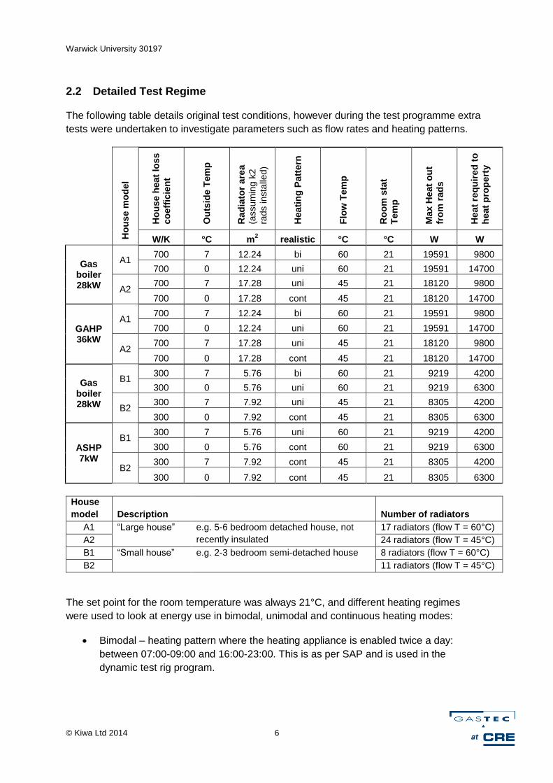
2.2 Detailed Test Regime
The following table details original test conditions, however during the test programme extra
tests were undertaken to investigate parameters such as flow rates and heating patterns.
Ho
use m
od
el
Ho
use h
eat
loss
co
eff
icie
nt
Ou
tsid
e T
em
p
Rad
iato
r are
a
(assum
ing
k2
rads insta
lled)
Heati
ng
Patt
ern
Flo
w T
em
p
Ro
om
sta
t
Tem
p
Max H
eat
ou
t
fro
m r
ad
s
Heat
req
uir
ed
to
heat
pro
pert
y
W/K °C m2 realistic °C °C W W
Gas boiler 28kW
A1 700 7 12.24 bi 60 21 19591 9800
700 0 12.24 uni 60 21 19591 14700
A2 700 7 17.28 uni 45 21 18120 9800
700 0 17.28 cont 45 21 18120 14700
GAHP 36kW
A1 700 7 12.24 bi 60 21 19591 9800
700 0 12.24 uni 60 21 19591 14700
A2 700 7 17.28 uni 45 21 18120 9800
700 0 17.28 cont 45 21 18120 14700
Gas boiler 28kW
B1 300 7 5.76 bi 60 21 9219 4200
300 0 5.76 uni 60 21 9219 6300
B2 300 7 7.92 uni 45 21 8305 4200
300 0 7.92 cont 45 21 8305 6300
ASHP 7kW
B1 300 7 5.76 uni 60 21 9219 4200
300 0 5.76 cont 60 21 9219 6300
B2 300 7 7.92 cont 45 21 8305 4200
300 0 7.92 cont 45 21 8305 6300
House
model Description
Number of radiators
A1 “Large house” e.g. 5-6 bedroom detached house, not
recently insulated
17 radiators (flow T = 60°C)
A2 24 radiators (flow T = 45°C)
B1 “Small house” e.g. 2-3 bedroom semi-detached house 8 radiators (flow T = 60°C)
B2 11 radiators (flow T = 45°C)
The set point for the room temperature was always 21°C, and different heating regimes
were used to look at energy use in bimodal, unimodal and continuous heating modes:
Bimodal – heating pattern where the heating appliance is enabled twice a day:
between 07:00-09:00 and 16:00-23:00. This is as per SAP and is used in the
dynamic test rig program.

Warwick University 30197
© Kiwa Ltd 2014 7
Unimodal – heating appliance is enabled for one period a day from 07:00 – 23:00.
Continuous – heating appliance is enabled for 24 hours a day.
For 24 hour testing it is important that the start and end conditions are the same; so to keep
the offset between the temperature of the property at the beginning and end to a minimum,
the starting temperature of the house was varied for each test. Calculations were performed
to find the optimum start temperature. The dynamic test rig was then left to operate in the
desired heating pattern for 24 hours.
The large house was a typical large and/or poorly insulated house that would use between
32,000 to 38,000kWh/y of heat depending upon the DHW demand. The small house is a
semi-detached moderately insulated house that might use 14,000 to 16,000kWh/y of heat
depending upon DHW demand. The gas boiler was sized at 28kW to provide a satisfactory
flow of instantaneous DHW for a shower.
2.3 Appliance Specifications
The following table shows, for the appliances under test, the manufacturers’ declared
thermal outputs and COP/efficiencies at specific external temperatures and flow
temperatures (shown in the table as A+7W50 = external air temperature of +7°C and water
flow temperature of 50°C). The gas boiler was a combi boiler. Boilers are tested according
to BED.
Efficiency (%) Thermal Power (kW)
Gas boiler
condensing mode 91.1* 30.3
non-condensing mode N/A 28
DHW mode N/A 33
GAHP
A+7W50 152 35.4
A+7W65 119 27.5
A-7W50 125 31.5
nominal output N/A 25.7
ASHP A+2W35 317 8.5
A+7W35 418 9.0
*This is the declared SEDBUK efficiency

Warwick University 30197
© Kiwa Ltd 2014 8
3 Results
Efficiency is calculated throughout this report using the following equations:
Efficiency of appliance = heat out from appliance / (gas in + electric in) (this is equivalent to the instantaneous efficiency or COP averaged over 24 hours)
Efficiency of system = heat out from radiators / (gas in + electric in) (this is equivalent to the system efficiency or SPFH4, assuming no buffer tanks or DHW use)
The electrical input includes all the pumps to reach the stated flow rate, the gas boiler has a
pump within the appliance box, however the other appliances require additional pumps
which run continuously no matter what the heating pattern. This will downgrade their
efficiency by 4-10% (see Section 4.1).
3.1 Gas boiler in Large House (700W/K)
Table 1: Results from gas boiler in the large house (700W/K)
Test
nu
mb
er
Ou
tsid
e T
(°C
)
Reg
ime
Flo
w (
m3/h
)
Flo
w T
(°C
)
Gas in
(k
Wh
)
Ele
ctr
ic in
(kW
h)
Heat
ou
t fr
om
ap
p (
kW
h)
Eff
icie
nc
y o
f
ap
plian
ce
*1
Heat
ou
t fr
om
rad
s (
kW
h)
Eff
icie
nc
y o
f
syste
m *
2
Mean
In
t T
(°C
)
080 7 Bi 1.0 60 196 3 196 99% 195 98% 18.2
083 0 Uni 1.0 60 325 4 317 97% 316 96% 18.5
092 *3 7 Uni 1.0 45 221 3 222 99% 221 99% 19.8
090 *3 0 Cont 1.0 45 342 4 342 99% 341 99% 20.9
*1 Equivalent to the instantaneous efficiency averaged over 24 hours.
*2 Assuming no domestic hot water (DHW) use.
*3 These tests have been corrected to allow for very high humidity and temperatures at the air inlet to the boiler, using the
methods described in the Good Laboratory Practice for full and part load efficiency measurement for boilers (Revision of the
document 1998-2000, Version 08, www.dgc.dk/labnet)

Warwick University 30197
© Kiwa Ltd 2014 9
Test number 080
Temperatures
Energy

Warwick University 30197
© Kiwa Ltd 2014 10
Test number 083
Temperatures
Energy

Warwick University 30197
© Kiwa Ltd 2014 11
Test number 092
Temperatures
Energy

Warwick University 30197
© Kiwa Ltd 2014 12
Test number 090
Temperatures
Energy
Warwick University 30197
© Kiwa Ltd 2014 13
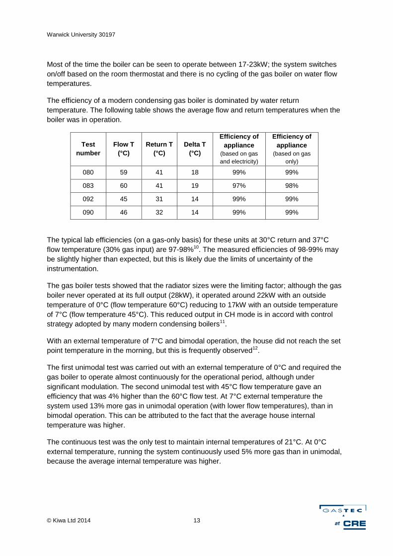
Most of the time the boiler can be seen to operate between 17-23kW; the system switches
on/off based on the room thermostat and there is no cycling of the gas boiler on water flow
temperatures.
The efficiency of a modern condensing gas boiler is dominated by water return
temperature. The following table shows the average flow and return temperatures when the
boiler was in operation.
Test
number
Flow T
(°C)
Return T
(°C)
Delta T
(°C)
Efficiency of
appliance
(based on gas
and electricity)
Efficiency of
appliance
(based on gas
only)
080 59 41 18 99% 99%
083 60 41 19 97% 98%
092 45 31 14 99% 99%
090 46 32 14 99% 99%
The typical lab efficiencies (on a gas-only basis) for these units at 30°C return and 37°C
flow temperature (30% gas input) are 97-98%10. The measured efficiencies of 98-99% may
be slightly higher than expected, but this is likely due the limits of uncertainty of the
instrumentation.
The gas boiler tests showed that the radiator sizes were the limiting factor; although the gas
boiler never operated at its full output (28kW), it operated around 22kW with an outside
temperature of 0°C (flow temperature 60°C) reducing to 17kW with an outside temperature
of 7°C (flow temperature 45°C). This reduced output in CH mode is in accord with control
strategy adopted by many modern condensing boilers11.
With an external temperature of 7°C and bimodal operation, the house did not reach the set
point temperature in the morning, but this is frequently observed12.
The first unimodal test was carried out with an external temperature of 0°C and required the
gas boiler to operate almost continuously for the operational period, although under
significant modulation. The second unimodal test with 45°C flow temperature gave an
efficiency that was 4% higher than the 60°C flow test. At 7°C external temperature the
system used 13% more gas in unimodal operation (with lower flow temperatures), than in
bimodal operation. This can be attributed to the fact that the average house internal
temperature was higher.
The continuous test was the only test to maintain internal temperatures of 21°C. At 0°C
external temperature, running the system continuously used 5% more gas than in unimodal,
because the average internal temperature was higher.

Warwick University 30197
© Kiwa Ltd 2014 14
3.2 Gas boiler in Small House (300W/K)
Table 2: Results from gas boiler in the small house (300W/K)
Test
nu
mb
er
Ou
tsid
e T
(°C
)
Reg
ime
Flo
w (
m3/h
)
Flo
w T
(°C
)
Gas in
(k
Wh
)
Ele
ctr
ic in
(kW
h)
Heat
ou
t fr
om
ap
p (
kW
h)
Eff
icie
nc
y o
f
ap
plian
ce
*1
Heat
ou
t fr
om
rad
s (
kW
h)
Eff
icie
nc
y o
f
syste
m *
2
Mean
In
t T
(°C
)
108 7 Bi 1.0 60 90 3 86 93% 86 93% 18.8
109 *3 7 Uni 1.0 60 101 3 97 93% 95 91% 20.3
106 0 Uni 1.0 60 141 3 133 93% 132 92% 19.0
099 7 Uni 1.0 45 97 3 96 96% 96 96% 20.0
103 0 Uni 1.0 45 137 3 136 97% 136 97% 18.9
188 0 Cont 1.0 45 148 6 148 96% 144 93% 20.9
*1 Equivalent to the instantaneous efficiency averaged over 24 hours.
*2 Assuming no domestic hot water (DHW) use.
*3 In addition to the original test regime, an extra test was undertaken at 7°C, under unimodal conditions.

Warwick University 30197
© Kiwa Ltd 2014 15
Test number 108
Temperatures
Energy

Warwick University 30197
© Kiwa Ltd 2014 16
Test number 109
Temperatures
Energy

Warwick University 30197
© Kiwa Ltd 2014 17
Test number 106
Temperatures
Energy

Warwick University 30197
© Kiwa Ltd 2014 18
Test number 099
Temperatures
Energy

Warwick University 30197
© Kiwa Ltd 2014 19
Test number 103
Temperatures
Energy
Warwick University 30197
© Kiwa Ltd 2014 20
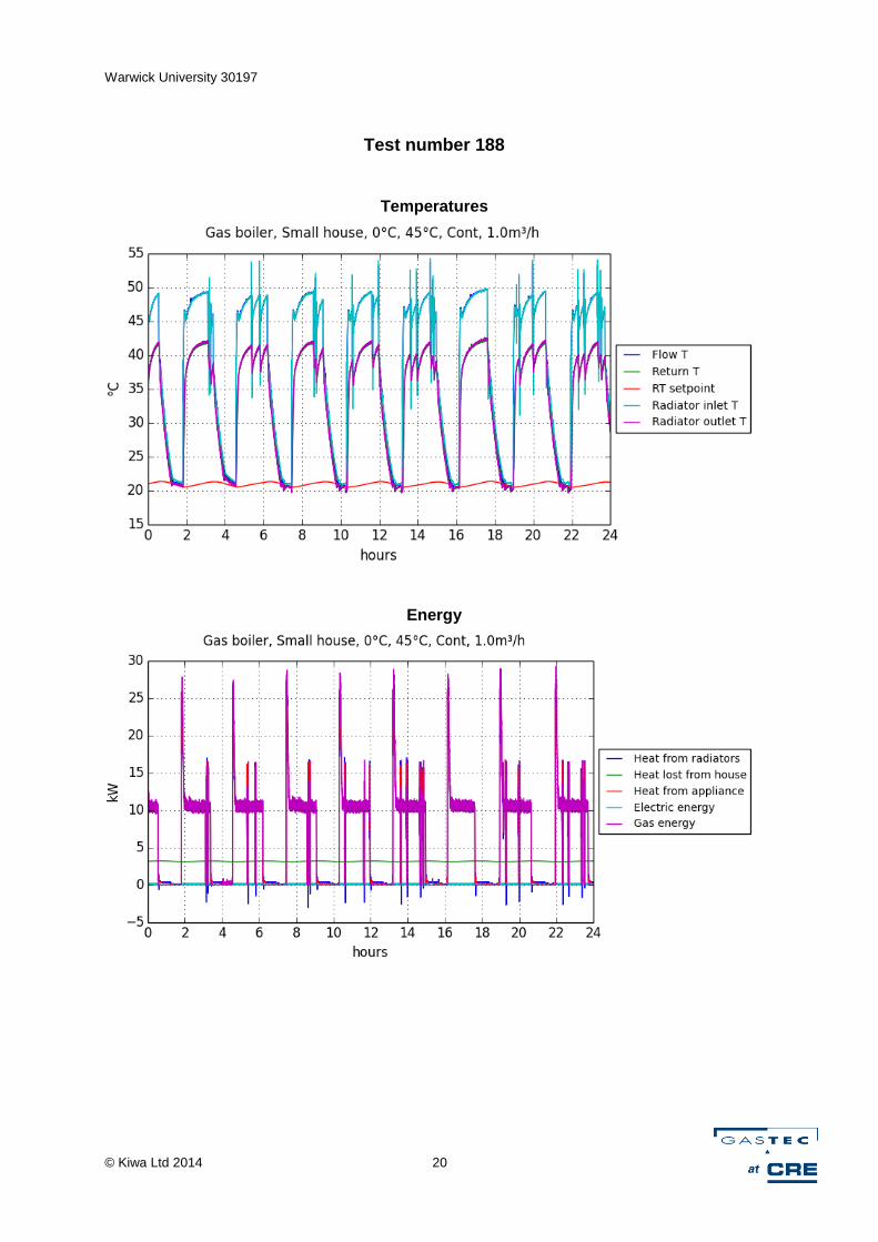
Test number 188
Temperatures
Energy

Warwick University 30197
© Kiwa Ltd 2014 21
Most of the time of boiler can be seen to operate between 10-14kW. In contrast with the
large house, when operated at a 45°C flow temperature, the boiler begins to cycle on water
flow temperature at a rate of 3 cycles/hour. The system also turned on/off more frequently
than in the large house. Both of these effects are expected, as in the smaller house there
will be a less water in the heating system, which will heat up more quickly; as the house has
a lower heat loss coefficient, it will also heat up more quickly.
The efficiencies were lower in these tests which may be as a result of the increased cycling.
Increased cycling leads to increased losses due to purging prior to ignition and loss of
unburnt gas during ignition. The radiator temperature for the 45°C tests can be seen to rise
to 50°C throughout each cycle before the gas boiler turned off and started back up again.
During start up the system efficiency was decreased as can be seen on the energy graph,
the gas boiler (pink, bottom graphs) ignites at ~28kW, and quickly falls to the limitation of
the radiator output (about 12kW).
This is the effect of cycling which decreases the efficiency and is more prevalent on warmer
days in spring and summer when the load is very light. As indicated above, the 28kW gas
boiler is designed to supply a shower and is not sized on central heating demand; it is
designed to modulate under normal CH use.
The radiator heat output was the limiting factor on this series of tests, with heat outputs
decreased to 15kW at 60°C and 12kW at 45°C.
House temperatures were limited both by radiator area and gas boiler output. Again with an
external temperature of 7°C, the house did not reach the set point temperature in the
morning.
Tests were carried out with outside air temperatures of 0 and 7°C and water temperatures
of 45 and 60°C. The efficiency was 4% lower when using flow temperatures of 60°C. As
expected the warmer day yielded higher average internal temperatures.
Continuous operation used 8% more gas than unimodal at 45°C and 5% more gas than
unimodal at 60°C. This is in good agreement with previous modelling of continuous and
unimodal operation, which suggested on average a 7-8% increase in gas use when moving
from unimodal to continuous heating13.

Warwick University 30197
© Kiwa Ltd 2014 22
3.3 ASHP in Small House (300W/K)
Table 3: Test results for ASHP in small house (300W/K)
Test
nu
mb
er
Ou
tsid
e T
(°C
)
Hu
mid
ity (
%)
Reg
ime
Flo
w (
m3/h
)
Flo
w T
(°C
)
Ele
ctr
ic in
(kW
h)
Heat
ou
t
fro
m a
pp
(kW
h)
24 h
Eff
icie
nc
y o
f
ap
plian
ce
*1
Heat
fro
m
rad
s (
kW
h)
24 h
Eff
icie
nc
y o
f
syste
m *
2
Mean
In
t T
(°C
)
115 7 — *4 Uni 1.0 60 34 97 289% 89 265% 19.5
124 0 60 Uni 1.0 60 56 140 251% 130 232% 17.7
120 7 — *4 Cont 1.0 60 37 110 295% 101 270% 20.9
122 0 59 Cont 1.0 60 66 162 245% 148 224% 20.8
132 7 58 Cont 1.0 45 32 105 330% 98 309% 20.9
129 *3
7 75 Cont 1.15 45 33 101 308% 96 293% 20.9
126 0 45 Cont 1.0 45 59 160 271% 150 254% 20.8
127 *3
0 47 Cont 1.15 45 57 152 266% 141 248% 20.7
*1 Equivalent to the instantaneous coefficient of the performance (COP) averaged over 24 hours.
*2 Equivalent to SPFH4, assuming there are no buffer tanks or domestic hot water (DHW) use.
*3 In addition to the original test regime, extra tests were undertaken with different flow rates.
*4 Measurement instrumentation issues, set point was 60%.

Warwick University 30197
© Kiwa Ltd 2014 23
Test number 115
Temperatures
Energy

Warwick University 30197
© Kiwa Ltd 2014 24
Test number 124
Temperatures
Energy

Warwick University 30197
© Kiwa Ltd 2014 25
Test number 120
Temperatures
Energy
Warwick University 30197
© Kiwa Ltd 2014 26
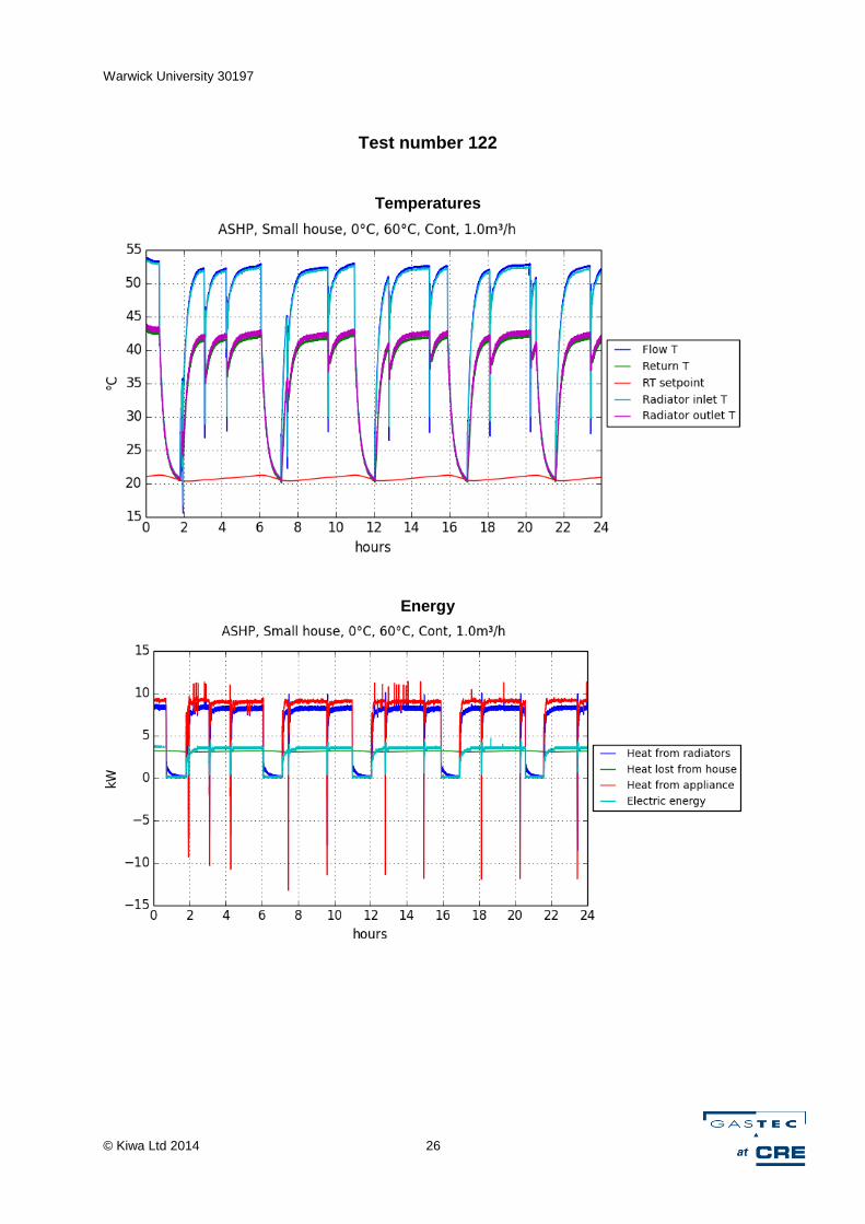
Test number 122
Temperatures
Energy

Warwick University 30197
© Kiwa Ltd 2014 27
Test number 132
Temperatures
Energy

Warwick University 30197
© Kiwa Ltd 2014 28
Test number 129
Temperatures
Energy

Warwick University 30197
© Kiwa Ltd 2014 29
Test number 126
Temperatures
Energy
Warwick University 30197
© Kiwa Ltd 2014 30
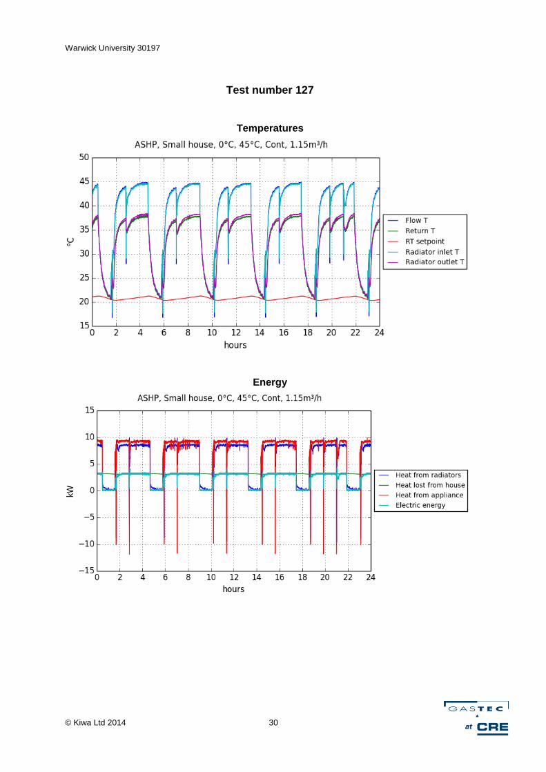
Test number 127
Temperatures
Energy

Warwick University 30197
© Kiwa Ltd 2014 31
The ASHP operated relatively continuously with heat output of 8-9kW, with little evidence of
cycling on water flow temperature. If the room temperature set point was reached then the
system switched on/off with a period of around 4-5 hours.
Defrost cycles are clearly visible as the electrical demand falls close to zero and the
appliance absorbs heat from the system (i.e. has a negative energy flow.) This defrosting is
very infrequent with an external temperature of +7⁰C, but is very evident at 0⁰C (for
example in test runs 124 and 127.)
The flow temperatures of 60°C required by a conventional radiator system were not
achieved with this ASHP (as anticipated). The highest temperature reached in the 60°C
(notional) tests was 54.3°C, with the mean flow temperature when the ASHP was running
(at 60°C notional) averaging between 48 and 49.8°C. This is because ASHPs do not
provide energy efficiently at high temperatures, to achieve high flow temperatures
supplementary/booster heaters would be required.
During the 45°C tests, it was found that the maximum temperature seen was 45.9°C while
the average temperature during operation was 42°C. This was because the ASHP took a
long time to get up to temperature. Attempting to reach these high water temperatures
inevitably reduces instantaneous COP.
It is interesting to compare these values with the manufacturer’s declared COP values; this
is shown in the figure below. In view of the difference in operating temperatures the results
are not unexpected. This does highlight that the effect of water flow temperature is
substantive.

Warwick University 30197
© Kiwa Ltd 2014 32
Comparison of manufacturer declared COP and experimental efficiencies
observed at different flow temperatures
Where multiple results exist at different flow rates these have been averaged
During the testwork, the ASHP was located in the temperature controlled environment
(‘blue box’) and the dynamic rig located within the adjacent laboratory building. This means
there was additional pipework, consisting of 2m in the blue box (at 0 or 7°C) +2.5m outside
(at ambient temperature) + 2m inside (at laboratory temperature 20°C). This appears to
equate to a difference in the delta T of 1°C, which is about 10kWh over the 24 hour test
period. This means the heat delivered to the radiators can be 0.8kW lower than the heat
supplied by the appliance. This is in many ways a reflection of reality in many ASHP
installations.
Defrost cycles were generally only observed when the external temperature was at 0°C,
however there was 1 defrost cycle on the unimodal 7°C cycle at flow temperature of
approaching 60°C, during the prolonged on-period.
The radiator sizes were not the limiting factors in these tests because the output was
generally approaching the ASHP manufacturer’s stated output of 8.5kW, so the output of
the ASHP was the limiting factor.
Warwick University 30197
© Kiwa Ltd 2014 33
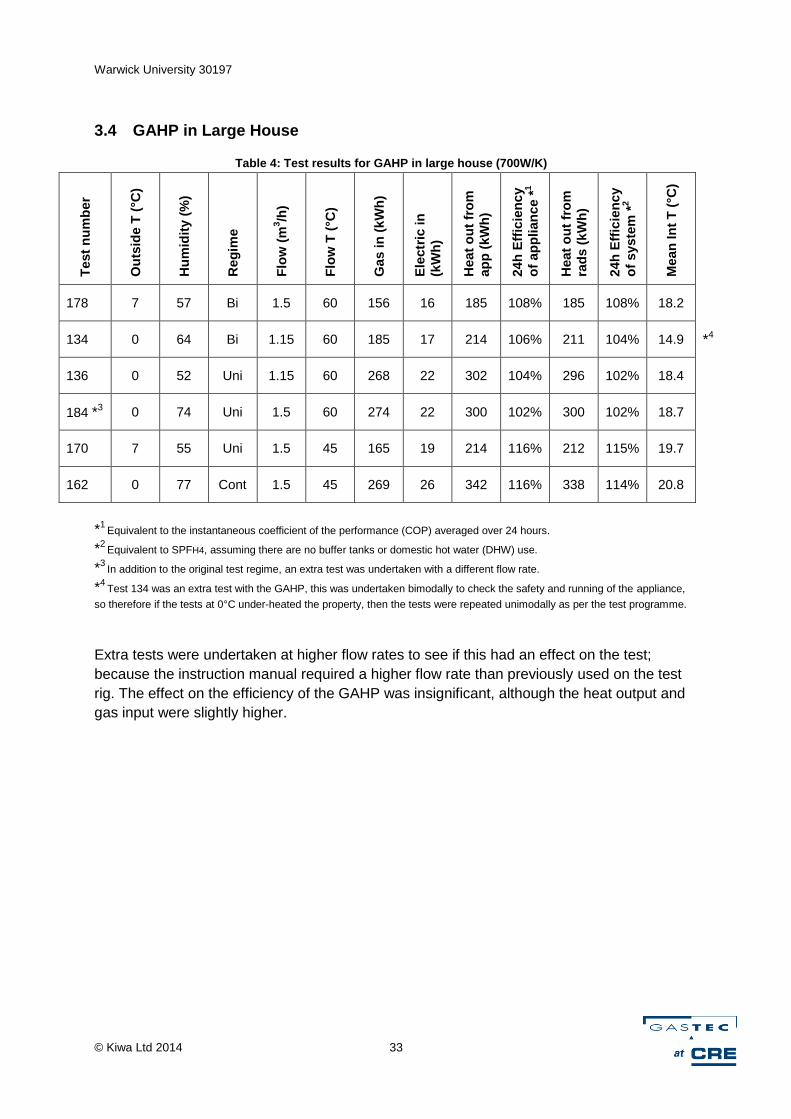
3.4 GAHP in Large House
Table 4: Test results for GAHP in large house (700W/K)
Test
nu
mb
er
Ou
tsid
e T
(°C
)
Hu
mid
ity (
%)
Reg
ime
Flo
w (
m3/h
)
Flo
w T
(°C
)
Gas in
(k
Wh
)
Ele
ctr
ic in
(kW
h)
Heat
ou
t fr
om
ap
p (
kW
h)
24h
Eff
icie
ncy
of
ap
plian
ce
*1
Heat
ou
t fr
om
rad
s (
kW
h)
24h
Eff
icie
ncy
of
syste
m *
2
Mean
In
t T
(°C
)
178 7 57 Bi 1.5 60 156 16 185 108% 185 108% 18.2
134 0 64 Bi 1.15 60 185 17 214 106% 211 104% 14.9 *4
136 0 52 Uni 1.15 60 268 22 302 104% 296 102% 18.4
184 *3 0 74 Uni 1.5 60 274 22 300 102% 300 102% 18.7
170 7 55 Uni 1.5 45 165 19 214 116% 212 115% 19.7
162 0 77 Cont 1.5 45 269 26 342 116% 338 114% 20.8
*1 Equivalent to the instantaneous coefficient of the performance (COP) averaged over 24 hours.
*2 Equivalent to SPFH4, assuming there are no buffer tanks or domestic hot water (DHW) use.
*3 In addition to the original test regime, an extra test was undertaken with a different flow rate.
*4 Test 134 was an extra test with the GAHP, this was undertaken bimodally to check the safety and running of the appliance,
so therefore if the tests at 0°C under-heated the property, then the tests were repeated unimodally as per the test programme.
Extra tests were undertaken at higher flow rates to see if this had an effect on the test;
because the instruction manual required a higher flow rate than previously used on the test
rig. The effect on the efficiency of the GAHP was insignificant, although the heat output and
gas input were slightly higher.

Warwick University 30197
© Kiwa Ltd 2014 34
Test number 178
Temperatures
Energy

Warwick University 30197
© Kiwa Ltd 2014 35
Test number 134
Temperatures
Energy

Warwick University 30197
© Kiwa Ltd 2014 36
Test number 136
Temperatures
Energy

Warwick University 30197
© Kiwa Ltd 2014 37
Test number 184
Temperatures
Energy

Warwick University 30197
© Kiwa Ltd 2014 38
Test number 170
Temperatures
Energy
Warwick University 30197
© Kiwa Ltd 2014 39
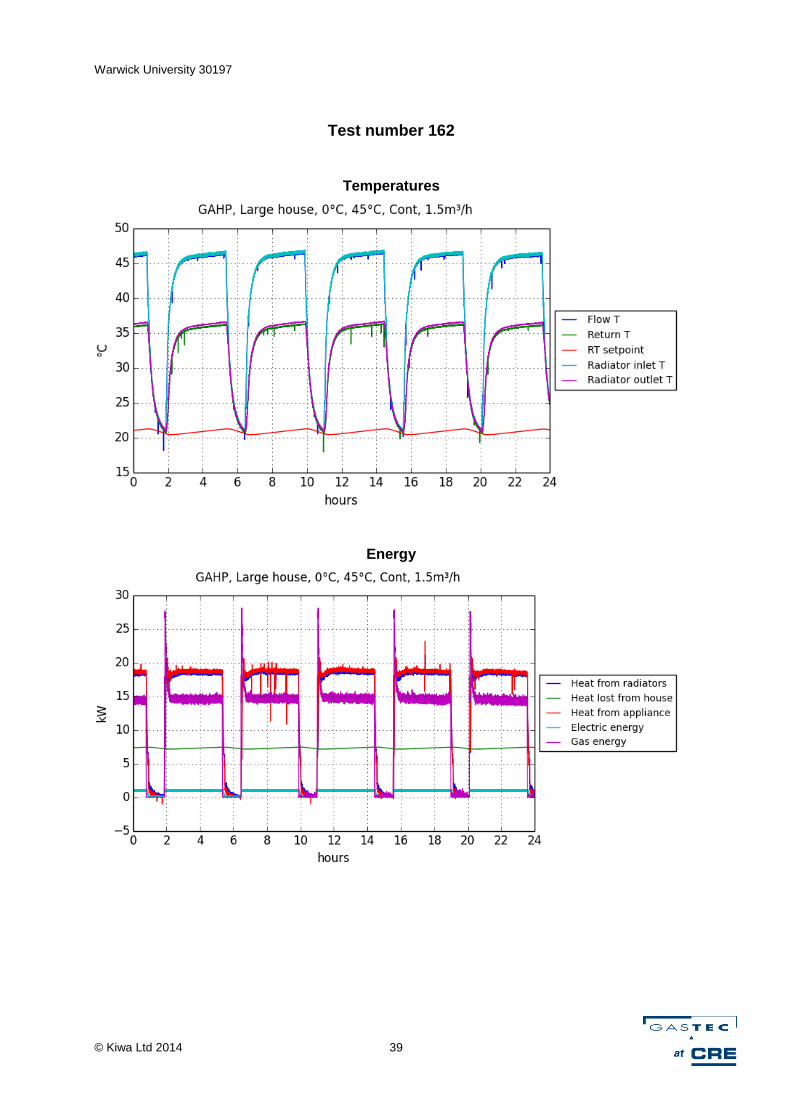
Test number 162
Temperatures
Energy

Warwick University 30197
© Kiwa Ltd 2014 40
The GAHP typically operated in the gas input range 14-22kW. There was no evidence of
cycling on water flow temperature. If the room temperature set point was reached then the
system switched on/off with a period of around 4-5 hours.
The radiator water flow rate for the GAHP was limited to a maximum of 1500l/h compared
to the recommended flow rate of 3000l/h, however the flow rate was higher than the
minimum 1000l/h. The flow rate was increased from 1150 to 1500l/h during the test for one
set of conditions (see tests 136 and 184), the effect on efficiency was insignificant.
The radiators were the limiting factor in the GAHP tests; at 14.9°C the internal temperature
could not be judged as acceptable in the bimodal tests at 0°C.
The efficiency was higher at lower flow temperatures than at higher flow temperatures. The
external temperature had less effect on the efficiency compared with an ASHP. The
manufacturer declared efficiencies for the GAHP are compared with the experimentally
determined efficiencies below.
The manufacturer declares efficiencies based on gas input (gross basis), so for comparison
purposes electricity use has been excluded from these efficiencies. Including electricity
would take on average 10% (expressed as percentage points) off these vales. This is an
argument for requiring manufacturers of GAHP to report efficiency including electricity.
Comparison of manufacturer declared efficiency and experimental
efficiencies observed at different flow temperatures
Efficiency calculated based on gas input (gross basis), neglecting electricity input
Where multiple results exist at different flow rates these have been averaged

Warwick University 30197
© Kiwa Ltd 2014 41
The efficiencies observed during testing at water flow temperatures of 60°C were consistent
with the manufacturer’s declared performance. At flow temperatures of 45°C, the efficiency
did not increase as much as predicted by the manufacturer data.
One reason for this reduced performance could be the gap (as discussed in Section 2.1.1)
between performance in laboratory testing (to a testing standard) and performance in the
‘real world’, and the associated lower efficiencies often observed there, due to the non-ideal
conditions experienced by the appliance.
It could be also argued the unit was oversized for the house size used during testing,
however this is a complex issue. There are advantages in using over-sized heat producers
as they allow bimodal heating (which as demonstrated in Section 3.2 can save significant
amounts of energy). By these criteria the unit was not unreasonably oversized when
compared to standard UK practice.
Table 5 compares the GAHP heating this 700W/K house to the 28kW gas combi boiler
heating the smaller 300W/K house (although in practice such boilers are usually down-rated
as low as 18kW when operating in central heating mode11).
Table 5: Comparison of load factors for GAHP and gas boiler
Large house
GAHP Small house Gas boiler
HLC W/K 700 300
Average internal temp C 19 19
Average outside temp C 2* 2*
Average heat load kW 11.9 5.1
Bimodal operating hours hours/day 9 9
Property demand kWh/day 286 122
Average heat output required kW 31.7 13.6
Design output of appliance in CH mode
kW 36 18
Ratio of design output to heat demand
113% 132%
* Chosen as an arbitrary cold day where the householder might not have switched to unimodal or
continuous heating.
The validity of this table can be demonstrated by comparing the similar unimodal operation
of the gas boiler and GAHP at both 0°C external temperature and radiators at 60°C (tests
083 and 136) and 7°C external temperature and radiators at 45°C (tests 092 and 170).
The energy flow graphs of the GAHP during start-up are similar to those of the gas boiler,
so it is suggested that the efficiency of the GAHP will be lower if the cycling is frequent,
because of purge etc. The GAHP however was not observed to cycle on flow temperature

Warwick University 30197
© Kiwa Ltd 2014 42
in any of the test programmes and typical operating times were 2 hours on and 2 hours off.
Such a control strategy is definitely beneficial.
The ability of a GAHP to provide large quantities of heat (like a boiler) is clearly
advantageous to bimodal heating of large properties and thus they could be ideal for
retrofitting into large and/or poorly insulted properties. There is however the complication
that achieving higher efficiencies requires low or even better very low water flow
temperatures. The latter necessitates underfloor heating or very large radiators, and
anecdotally there is an issue with consumer resistance to radiators (which intrinsically must
have high surface heat transfer coefficient and high thermal mass) that feel cold to the
touch, i.e. are operating at below body heat14.

Warwick University 30197
© Kiwa Ltd 2014 43
4 Discussion
4.1 Difference between laboratory, dynamic rig and field data
The measured efficiencies on the dynamic test rig for the gas boiler are significantly higher
than the seasonal efficiencies seen in field trials (which are typically 86±2%9) because:
field trials include DHW production, generally at poor efficiencies of ~70 to 75%
in a domestic property the gas boiler may not be correctly sized to the load and
radiators
this gas boiler had good modulation
the water flow temperatures of 60°C and 45°C are significantly lower than the 70-
80°C conventionally used in traditional radiator systems
higher water return temperatures due to spill back
The ASHP efficiency is lower on the dynamic test rig than in laboratory field tests. This is
partly due to the dynamic test rig requiring two pumps to achieve the flow rates expected.
These pumps equate to 110W with the standard flow rates, and 190W for the higher flow
rates. They run continuously no matter what the heating pattern. This has a significant
impact on the efficiency of the ASHP, downgrading the efficiency by 4-10%. Other effects
could be:
higher water flow/return temperatures than employed in the standard – laboratory
tests are undertaken at 35°C, the dynamic rig tests were undertaken at 45°C and
higher
effect of defrost
With the GAHP there is a significant discontinuity between the results observed here and
those achieved in the EN tests at the lower emitter temperature. Interestingly, data from
Kiwa Gastec in the Netherlands indicates efficiencies of 120% are typical for field
installations of GAHP15. A few reasons for this could be:
the dynamic operation
higher water flow/return temperatures than employed in the standard
the pumps account for 2-4% of the difference in efficiency, depending on whether
the field installation includes pumps
effect of defrost
4.2 Primary Energy and Carbon Emissions
The primary energy (in kWh) has been calculated from the gas and electricity consumption,
assuming electricity is supplied from a combined cycle gas turbine with an efficiency of
47.7%1. This is used to produce a heat to energy ratio (the efficiency) and a heat to primary
energy ratio for each different set of conditions.
This assumes that all the electricity consumed is generated by combined cycle gas turbine
which is the most efficient type of fossil fuel power station. With the current mix of coal

Warwick University 30197
© Kiwa Ltd 2014 44
generation in the UK, the primary energy consumption of the ASHP (and also the GAHP),
may be higher.
The equivalent CO2 emissions (per kWh of heat output) were also calculated, assuming
emissions factors of 0.5173 kgCO2e/kWh for electricity and 0.1841 kgCO2e/kWh for gas3.

Warwick University 30197
© Kiwa Ltd 2014 45

Warwick University 30197
© Kiwa Ltd 2014 46

Warwick University 30197
© Kiwa Ltd 2014 47

Warwick University 30197
© Kiwa Ltd 2014 48

Warwick University 30197
© Kiwa Ltd 2014 49
The following tables compare total carbon emissions to maintain a property at the declared
average internal temperatures (shown in brackets) when the external temperatures are 0⁰C
and 7⁰C. For comparison UK field trials show average internal temperatures in the range
17.7⁰C 2.
Daily carbon emissions (kgCO2e/day)
(Average internal temperature (°C))
Small house (300W/K) Large house (700W/K)
External temp 0⁰C Boiler ASHP Boiler GAHP
Bimodal Rads 60⁰C N/T N/T N/T N/T
Bimodal Rads 45⁰C N/T N/T N/T N/T
Unimodal Rads 60⁰C 27.5 (19.0)
29.0 (17.7)
61.7 (18.5)
60.6 (18.4)
Unimodal Rads 45⁰C 26.9 (18.9)
N/T N/T N/T
Continuous Rads 60⁰C N/T 34.2 (20.8)
N/T N/T
Continuous Rads 45⁰C 30.5 (20.9)
30.5 (20.8)
65.0 (20.9)
63.1 (20.8)
External temp 7⁰C Boiler ASHP Boiler GAHP
Bimodal Rads 60⁰C 17.9 (18.8)
N/T 37.5 (18.2)
37.1 (18.2)
Bimodal Rads 45⁰C N/T N/T N/T N/T
Unimodal Rads 60⁰C 20.0 (20.3)
17.4 (19.5)
N/T N/T
Unimodal Rads 45⁰C 19.4 (20.0)
N/T 42.4 (19.8)
40.2 (19.8)
Continuous Rads 60⁰C N/T 19.3 (20.9)
N/T N/T
Continuous Rads 45⁰C N/T 16.4 (20.9)
N/T N/T
Key: N/T = Not tested as would not be realistic of operation of the appliance in the field.
Reasons for this may include: there would be insufficient heat output from the appliance to meet the heat
demand of the house, the radiators would be too small to deliver sufficient energy to the house, or the
appliance would cycle too frequently.
The equivalent CO2 emissions were calculated, assuming emissions factors of
0.5173 kgCO2e/kWh for electricity and 0.1841 kgCO2e/kWh for gas16. The ASHP could not
achieve the 60°C radiator temperatures. More detailed notes are given in the results.
Inspection of the results shows the extreme complexity of the values with both bimodal
operation and lower radiator temperatures lowering emissions, but in so doing making
comparison between heating systems very difficult.

Warwick University 30197
© Kiwa Ltd 2014 50
The report highlights the need to consider 5 factors when assessing the performance of a
heating system:
1. The ability of the system to operate bimodally, unimodally or continuously whilst
giving acceptable internal temperatures
2. System water temperature (especially return)
3. The instantaneous and average efficiency of the appliance in terms of both gas and
electricity
4. Ability to respond to external temperature
5. The carbon emissions of the above operating regime
To give undue weight to any one of these factors (for example appliance efficiency) is likely
to only yield part of the picture.
In the large house the GAHP used slightly less primary energy than the gas boiler to give
the same notional comfort level. The electricity use of the GAHP was higher than the
electricity use of the gas boiler especially once both circulating pumps were added in. On
the continuous test, the GAHP used 26kWh of electricity compared with 4kWh of electricity
used by the gas boiler, but the overall efficiency of the system was 114% with the GAHP
compared with 99% with the boiler. In terms of primary energy use, the ratio of heat to
primary energy was 106% with the GAHP compared with 98% with the gas boiler, and the
carbon emissions were 0.184kgCO2e/kWh with the GAHP compared with
0.190kgCO2e/kWh with the gas boiler.
Both the GAHP and gas boiler in the large house were limited by the radiators in the 7°C
bimodal test. The room temperature averaged 18.2°C for this test; the gas boiler and GAHP
had similar outputs from the radiators to achieve this, however the GAHP was more
efficient than the gas boiler.
In the large house, the GAHP had thermal efficiencies between 8-17 percentage points
higher (13 percentage points higher on average) than the gas boiler. In terms of carbon
emissions the reduction was only 1-5% (3% on average). The reason for the small
reduction in carbon emissions is the proportionally higher carbon footprint of electricity.
For the large house the ASHP was not tested as it had insufficient output to match the
property. In reality, a number of ASHP units would likely be used in combination to fully
satisfy the heat demand, although standard domestic wiring might be insufficient to meet
the electrical requirements of this set-up.
4.3 Timed heating
During bimodal heating the property is heated morning and evening as is typical in the UK.
House temperatures are limited either by radiator area and/or heating appliance output.
With an external temperature of 7°C the house does not reach the set point temperature in
the morning. This is typical and is consistent with previous laboratory tests12. The set up
(i.e. gas boiler, radiators and time clock settings) maintains a mean internal temperature

Warwick University 30197
© Kiwa Ltd 2014 51
above 18.2°C throughout the day. This is typical when compared to that seen in real
properties9.
In the small house boiler test, continuous operation used 8% more gas than unimodal at
45°C and 5% more gas than unimodal at 60°C.
This demonstrates that:
Switching the gas boiler off for 15 hours/day (i.e. bimodal operation) makes
worthwhile savings in daily energy use, if the property can still be comfortably lived
in.
Operating the gas boiler in the small house at 45°C rather than 60°C makes 4%
difference to gas demand and efficiency.
Daily gas use is dominated by average house temperature and average gas boiler
efficiency but the latter (on a modern condensing gas boiler) is constrained (for
central heating production) in a relatively narrow range around 90 to 95%.
In the case of the smaller house, the balance of carbon emissions between the gas boiler
and the ASHP becomes fine with the ASHP showing an advantage at 7°C, and the gas
boiler an advantage at 0°C. However both are dependent upon radiator temperature – with
radiators designed at 45°C (i.e. a 3.1 oversize factor on their normal rating) and an external
temperature of 7°C, the ASHP carbon saving does become more significant – up to 15%.

Warwick University 30197
© Kiwa Ltd 2014 52
5 Conclusions
The GAHP was compared against a broadly similar sized condensing gas boiler; the same
gas boiler was used for comparisons with the ASHP as this would represent the common
situation of a condensing combination gas boiler, where the output rating is determined by
the instantaneous hot water demand rather than the space heating demand.
Compared with ASHPs, GAHPs have the advantage of being able to deliver heat in large
quantities and at higher temperatures, which may allow installations in existing installations
with fewer modifications to the property. However, truly domestic scale GAHPs are still in
development. The unit tested here might have been better suited to very large houses or
commercial applications, although strictly the GAHP was no more oversized than the typical
gas combi boiler in a typical property.
All of the systems have to be viewed holistically. Just measuring efficiency is not really
meaningful. This insight explains the widespread differences in energy consumption
between apparently similar properties.
This work highlights the fact that using different heating patterns with different appliances
can markedly affect both the reported efficiency and the actual energy used. A higher
efficiency for the appliance may not save primary energy, if the methodology used to obtain
the high efficiency results in the building remaining at a higher average temperature and
thus using more primary energy.
In terms of actual energy used and primary energy used, high quality, well installed ASHPs
show themselves to be an effective method of reducing energy use and carbon emissions
in central heating applications with primary energy savings over a the gas combi of up to
20% at 0°C with radiators at 60°C, and rising to 32% at 7°C with radiators at 45°C, over the
scenarios studied. It should be noted however that in conjunction with these savings, there
may be a change in the average internal temperature of the house. Further changes may
also be required such as the installation of additional radiators to enable lower flow and
return temperatures to be used. This may result in changes to the level of comfort
experienced by the householder. The large scale introduction of this technology is also
limited by both grid capacity and installed cost.
In the interim GAHPs should have a role to play in saving energy and balancing the
demand between gas and electric over the coming years with primary energy savings over
a the gas combi of up to 6% at 0°C with radiators at 60°C, and rising to 10% with radiators
at 7°C with radiators at 45°C, over the scenarios studied. Design, installation and control
have been shown to be important and this should also be considered. Further development
of GAHPs should result in improved performance as the technology matures and also
optimisation for UK conditions (climate and usage patterns) could bring benefits.
The data shows that there is still much to be understood about heat sources, emitters and
optimum operating regime.
Warwick University 30197
© Kiwa Ltd 2014 53
6 Further work
There are currently no small output GAHPs available in the UK so the technology could not
be tested in the smaller property, but the data would indicate that there should be primary
energy savings over the gas boiler. This would combine the potential benefits of rapid heat
up with higher efficiencies than gas boilers using the same infrastructure that is currently
established in the UK. They could even be regarded as merely a further step in the long
term development of the gas boiler from traditional open-flued, to high efficiency fan flued,
to fan flued condensing boiler and eventually to gas-fired heat pump.
This work has not touched upon the effect of radiative vs convective heat in relation to
householder comfort. Anecdotes and Dutch data17 provide some evidence that higher
temperature emitters permit lower air temperatures for the same level of “comfort”. This
may explain why some householders find bimodal heating (when the radiators are always
hotter morning and evening) more comfortable than might be expected.
It should be noted that this work also excluded the effect of DHW production. In general,
DHW is produced and supplied at relatively high temperatures (60°C to 65°C). Requiring
higher temperatures is likely to increase the primary energy use of all three technologies. It
is anticipated that the most affected technology would be the ASHP, due to the high flow
temperatures required for DHW which are often unachievable without supplementary
heaters. The GAHP has not been tested for DHW production so this cannot be compared to
the gas boiler.
This work modelled standard radiators; underfloor heating is conventionally associated with
continuous heating, although underfloor heating systems can use a night set back. The
lower flow temperatures required by underfloor heating could increase efficiencies but may
be significantly affected by DHW production. More work is required on the basis of primary
energy per property per year. There are also issues with the relative responsiveness of
radiators and underfloor heating in concrete screed.
When evaluating the relevance of laboratory testing standard results, it is useful to consider
the actual load factor experienced by an appliance in the UK. This load factor can be
calculated from the monthly degree day heating* requirement, shown in the figure below
* Degree days heating are a measure of the deficit between the average daily outside temperature and a ‘base temperature’
(below which the property requires no heating). More information is available at: www.vesma.com/ddd

Warwick University 30197
© Kiwa Ltd 2014 54
Typical UK monthly degree day heating requirement18
Design degree day values are typically 700 to 750 DDH in the UK. It can be seen from the
figure above that boiler load factors can be less than 10% for 4 months of the year, and less
than 30% for around 8 months of the year. Therefore it is vital that any technology new to
the UK can operate efficiently at low load or when only called upon to operate very
intermittently.
This is why PAS674, the UK test protocol for mCHP units, contains a requirement to test at
10% daily load (i.e. 2.4 hours/day). A very similar approach is developed within the new
BSEN14825:2013. (Air conditioners, and heat pumps... testing and rating at part load
conditions and calculation of seasonal performance). Whilst always assuming continuous
heating this allocates heating and cooling into temperature bins and then sums these to
produce an annual performance (termed a seasonal COP or SCOP). This standard does
endeavour to model the effect of load factor, but many of the measurements are non
mandatary so how accurately the results reflect reality is still to be proven. (It is noted that
that the GAHP tested is promoted as a base load unit, although this will tend to limit its
application, as many large heating systems which might incorporate such base load
appliances tend to operate with water temperatures above the 45°C necessary to obtain the
highest efficiencies.)
This whole area could benefit from further research and perhaps consideration of the
introduction of a 24 hour test programme that would test heat pumps at 100%, 30% and
10% of thermal rating to report their response to low loads. Although at first sight complex,
PAS67 does have the advantage of offering the manufacturer a range of recommended
operating regimes, e.g. bimodal, unimodal and continuous.
Many mCHP manufacturers have found that investigating performance under these
conditions yields considerable improvements in appliance performance; it has also saved
them from the poor publicity likely to arise from mCHP installations that operate
0
100
200
300
400
500
Jan
Fe
b
Ma
r
Apr
Ma
y
Jun
Jul
Aug
Sep
Oct
No
v
De
c
Mo
nth
ly d
eg
ree d
ay
heati
ng
req
uir
em
en
t

Warwick University 30197
© Kiwa Ltd 2014 55
disproportionately poorly at low load. There could be parallels with GAHPs here, as both
technologies have to establish equilibrium of their working fluids to achieve optimum output.

Warwick University 30197
© Kiwa Ltd 2014 56
References
1 Department of Energy & Climate Change. Digest of UK energy statistics 2013. ISBN 9780115155291. Table 5.10 Thermal
efficiency – Combined cycle gas turbine stations (2012 value) 2 Department of Energy & Climate Change. The Future of Heating: A strategic framework for low carbon heat in the UK. 29
th
March 2012 3 Department of Energy & Climate Change. Green Book supplementary guidance: valuation of energy use and greenhouse
gas emissions for appraisal. Tables 1-20: supporting the toolkit and the guidance. 16th September 2013. Table 1: Electricity
emissions factors to 2100 (2013 grid average, consumption-based, domestic value) and Table 2a: Converting fuel types to CO2 and CO2e (Natural Gas, kgCO2e/kWh, 2013 value)
4 PAS 67:2013. Laboratory tests to determine the heating and electrical performance of heat-led micro-cogeneration
packages primarily intended for heating dwellings. ISBN 9780580837104 5 Robur. E3 A product literature. December 2013. Up to 165% (net basis)
6 R.E. Critoph. Private correspondence. 2013
7 Redpoint Energy. Gas Future Scenarios Project – Final Report. A report on a study for the Energy Networks Association
Gas Futures Group. November 2010 8 BS EN 14511-2:2013. Air conditioners, liquid chilling packages and heat pumps with electrically driven compressors for
space heating and cooling 9 GASTEC at CRE, AECOM and EA Technology. In situ monitoring of efficiencies of condensing boilers and use of
secondary heaters trial – final report. June 2009. GaC3563 10 UK Product Characteristics Database. SEDBUK boiler efficiency data 11
Industry stakeholders. Private correspondence 12
GASTEC at CRE. Optimisation of boiler water flow temperatures using a dynamic test rig. June 2011. GaC3933 13
GASTEC at CRE. Comparison of Bimodal, Unimodal and Continuous Heating Patterns: GASTEC dynamic test rig
simulations. February 2009. GaC3563/200902/01 14
Industry stakeholders. Private correspondence 15
Kiwa Gastec Netherlands. Private correspondence 16
Department of Energy & Climate Change. Green Book supplementary guidance: valuation of energy use and greenhouse
gas emissions for appraisal. Tables 1-20: supporting the toolkit and the guidance. 16th September 2013. Table 1: Electricity
emissions factors to 2100 (2013 grid average, consumption-based, domestic value) and Table 2a: Converting fuel types to CO2 and CO2e (Natural Gas, kgCO2e/kWh, 2013 value)
17 Kiwa Gastec Netherlands. Private correspondence
18 V. Vesma. Degree Day Data. www.vesma.com/ddd


![Gas Absorption[1]](https://static.documents.pub/doc/80x56/577c86ba1a28abe054c263df/gas-absorption1.jpg)


