Comparative Valuation Dynamics in Models with Financing Restrictions * Lars Peter Hansen University of Chicago [email protected]Paymon Khorrami University of Chicago [email protected]Fabrice Tourre Northwestern University [email protected]June 27, 2018 Abstract This paper develops a theoretical framework to nest many recent dynamic stochastic general equilibrium economies with financial frictions into one common generic model. Our goal is to study the macroeconomic and asset pricing properties of this class of models, identify common features and highlight areas where these models depart from each other. In order to characterize the asset pricing implications of this family of models, we study their term structure of risk prices and risk exposures, the natural extension of impulse response functions in economic environments exhibiting non-linear behaviors. * First draft February 2018. We thank Joseph Huang for excellent research assistance, and Amy Boonstra for her unconditional support. We would like to gratefully acknowledge the Macro-Finance Modeling initiative for their generous financial support. For their feedback, we thank the conference participants at the 2nd Research Conference of the MMCN, seminar attendees at Northwestern University, and participants at the Economic Dynamics Working Group at the University of Chicago.
Transcript
Comparative Valuation Dynamics inModels with Financing Restrictions∗
This paper develops a theoretical framework to nest many recent dynamic stochastic
general equilibrium economies with financial frictions into one common generic model.
Our goal is to study the macroeconomic and asset pricing properties of this class of
models, identify common features and highlight areas where these models depart from
each other. In order to characterize the asset pricing implications of this family of
models, we study their term structure of risk prices and risk exposures, the natural
extension of impulse response functions in economic environments exhibiting non-linear
behaviors.
∗First draft February 2018. We thank Joseph Huang for excellent research assistance, and Amy Boonstrafor her unconditional support. We would like to gratefully acknowledge the Macro-Finance Modeling initiativefor their generous financial support. For their feedback, we thank the conference participants at the 2ndResearch Conference of the MMCN, seminar attendees at Northwestern University, and participants at theEconomic Dynamics Working Group at the University of Chicago.
In this paper, we develop a theoretical framework and diagnostic tools for comparing and con-
trasting dynamic macroeconomic models with financial frictions. The literature studying this
class of models has expanded considerably following the 2008 financial crisis, as researchers
are trying to understand how financial intermediaries facing different types of regulatory and
contractual constraints influence macroeconomic outcomes.1 To what extent do the existing
models differ in their macroeconomic and asset pricing implications? To what extent are
they similar? Those questions are the key drivers motivating our research and prompting us
to undertake a comparison exercise.
To perform comparisons in a systematic way, we pose a theoretical continuous-time dy-
namic stochastic general equilibrium model that nests several benchmark models from the
literature. We focus on a production economy with two types of agents having different
productivities, preferences, and financial constraints. We follow previous research by intro-
ducing a productive role for the financing of investments by one class of agents meant to
capture financial intermediaries and their managers. These agents are more productive and
more risk tolerant than households, but they also face financing restrictions. These restric-
tions include limits on short-sales, equity issuance, and leverage. The occasionally binding
nature of those constraints generate an important source of nonlinearity in our model. We
allow both agent types to hedge aggregate risk exposures in financial markets, but subject
to constraints. Finally, we augment standard productivity shocks with growth-rate shocks,
aggregate volatility shocks, and idiosyncratic volatility shocks.
This set of assumptions results in an economic environment that nests multiple models
within a common setup to support model comparisons. Although this general nesting model
is less analytically tractable and more computationally complex than any of the benchmark
1Beginning from the seminal “financial accelerator” papers of Kiyotaki and Moore (1997) and Bernanke,Gertler, and Gilchrist (1999), there has been explosive growth in the literature on macroeconomic dynamicsunder financial frictions. See Brunnermeier and Sannikov (2014), He and Krishnamurthy (2012, 2013, 2014),Adrian and Boyarchenko (2012), Moreira and Savov (2017), Phelan (2016), Di Tella (2017), and Klimenkoet al. (2016) for some of the core issues in continuous-time models. An even more developed asset pricing lit-erature that predates the continous-time macro literature explores similar frictions in endowment economies:e.g., Basak and Cuoco (1998), Basak and Croitoru (2000), Basak and Shapiro (2001), Gromb and Vayanos(2002), Kondor (2009), Garleanu and Pedersen (2011). This set of macro-finance models has been extendedto examine conventional monetary theory (Drechsler, Savov, and Schnabl (2018), Brunnermeier and Sannikov(2016a), Di Tella and Kurlat (2017)), unconventional monetary policy (Silva (2016)), macro-prudential poli-cies (Di Tella (2016), Caballero and Simsek (2017)), international capital flows (Brunnermeier and Sannikov(2015)), and the cross-section of asset prices (Dou (2016)). For the recent wave of related discrete-time mod-els, see Gertler and Karadi (2011), Gertler and Kiyotaki (2010), Mendoza (2010), Bianchi (2011), Gertler andKiyotaki (2015), Christiano, Motto, and Rostagno (2014). For empirical work linking financial intermediaryleverage and net worth to asset prices and macroeconomic conditions, see Adrian and Shin (2010), Adrianand Shin (2013), Adrian, Etula, and Muir (2014), He, Kelly, and Manela (2017), Muir (2017), Siriwardane(2016).
1
models from the literature, our nesting framework offers two important advantages. First,
performing comparisons across models is complicated by the fact that each model has its
own special auxiliary assumptions and its own calibration. By nesting several models, we
can hold fixed auxiliary assumptions and parameters, using only a single parameter to tran-
sition from one model to another. This simplifies the comparison exercise. Second, nesting
different models necessarily introduces interactions between their assumptions. For example,
by nesting models “A” and “B”, our model allows us to solve a version of model “A” with
some of the features from model “B”, say its shock or preference structure. These interac-
tions help us distinguish between various assumptions on financial frictions, and allow us to
uncover new mechanisms not previously explored by previous articles in this literature.
To perform comparisons, we focus our attention on the asset-pricing implications of our
model. Like most of the literature, we characterize asset prices by the model’s stochastic dis-
count factor (SDF). Unlike complete markets’ environments, our model features two SDFs,
arising from the different investment opportunity sets faced by the two investor types. Invest-
ment opportunity sets differ since the two types of agents have different productivities and
face potentially heterogeneous sets of constraints. We contrast these SDFs to understand the
effects of financial frictions onto the compensations for aggregate risks earned by our different
agents.
We characterize the dynamics of the SDFs through their short-run dynamics, but we
supplement these with horizon-dependent diagnostics as well. Short-run dynamics of an
SDF St are summarized by its drift and diffusion (µS, σS), which pin down locally risk-free
investment returns as well as local risk prices. But these short-run diagnostics miss potentially
interesting intermediate- and long-horizon asset return properties. We thus augment the
standard asset-pricing analysis with a computation of term structures of risk prices, which
represent Sharpe ratios for dividend strips with various maturities. Our term structures are
characterized using the recently-developed shock elasticities’ tool kit.2 They provide a useful
joint summary of a model’s state dynamics and asset prices at different horizons. Importantly,
they give us another diagnostic tool to help distinguish various models.
At the same time, shock elasticities can be interpreted as nonlinear impulse response func-
tions.3 For instance, shock exposure elasticities for a given cashflow give us the sensitivity
of such expected future cashflow to a normalized shock occuring today, and in the context
of linear models with a Gaussian shock structure, they are identical to impulse response
functions. Using those shock elasticities to parse the underlying economics of financial fric-
tions’ models can thus bring this literature somewhat closer to the traditional macroeconomic
2See Borovicka et al. (2011), Hansen (2012), Hansen (2013). An accessible review treatment is providedin the handbook chapter Borovicka and Hansen (2016).
3See Borovicka, Hansen, and Scheinkman (2014).
2
DSGE literature. Indeed, the macro-finance literature with frictions has until now mostly
focused on short-run dynamics and long-run averages. In a stationary equilibrium with state
vector Xt, short-run dynamics are described by drift and diffusion coefficients (µX , σX), while
long-run outcomes are characterized by the stationary distribution p(x). Less often studied
are medium-run transition distributions pt(x) and how they vary with time t. Because of
their impulse response interpretation, shock elasticities provide a concise way to summarize
a model’s medium-run dynamics. For example, in nonlinear environments like ours, shock
elasticities can be informative about the term structure of crisis and recovery probabilities,
among other things.
We cast our model in continuous time, consistent with many recent papers in this liter-
ature. Continuous-time models with Brownian information are tractable due to their local
normality and localized transition dynamics. These features often deliver quasi-analytical
expressions for decision rules, allowing numerical procedures to avoid maximization steps.
Such expressions remain available even when optimization problems involve financial con-
straints, as in our model. Even more important, localized transition dynamics imply a sparse
transition matrix for the numerically discretized model, which greatly reduces computational
costs. Finally, global solutions methods can be easier to implement in continuous time be-
cause occasionally-binding constraints and highly nonlinear dynamics in extreme parts of the
state space boil down to an analysis of boundary conditions. Global solutions allow us to
evaluate the importance of various models’ nonlinearities and constraints.
We view part of our contribution as delivering a robust numerical solution method for
a high-dimension non-linear stochastic general equilibrium model with occasionally-binding
financial constraints. The equilibrium of our model reduces to a pair of coupled, nonlinear,
second-order partial differential equations for agents’ value functions, which have dimension
equal to the number of state variables in the model. We solve these equations with an
implicit finite difference scheme. In doing so, we take the standard approach of inserting the
PDE nonlinearities into an iterative step, by augmenting the time-independent PDEs with
a false time-derivative. At each iterative step, the discretized implicit scheme yields a large
linear system to solve. The sparsity offered by continuous time delivers speed gains, but to
speed things up even further, we leverage parallelization techniques and high-performance
computing packages in C++.4 Occasionally-binding constraints partition the state space into
regions where constraints bind and where they are slack. Such partitions are endogenous
hyper-surfaces in our state space, and solving for them numerically is a notoriously hard
problem. We tackle this issue by employing another iterative procedure, embedded within
4For example, we have used Pardiso (https://www.pardiso-project.org/) for fast LU decompositionsof our linear system.
the time-iterations for the PDEs. In particular, we iterate back and forth between agents’
Euler inequalities and market clearing conditions until both equilibrium prices and these
endogenous hyper-surfaces converge.
2 General Model
The model presented below is set in continuous time, t ∈ [0,∞). It builds on the model of
Brunnermeier and Sannikov (2016b), adding heterogeneous recursive preferences, overlapping
generations of agents, an exogenous TFP growth rate, both aggregate and idiosyncratic
volatility shocks, and additional types of financial frictions.
Technology. There are two types of agents, experts and households, denoted by e and
h, respectively. Each group has a continuum of agents indexed by j; the sets of experts
and households are denoted by Je and Jh, respectively. Because of competition and homo-
geneity assumptions we introduce later, it suffices to consider a representative expert and a
representative household.
Each agent produces output with a constant returns-to-scale technology taking only
quality-adjusted capital as an input. In particular, an agent with kj,t units of capital produces
ajkj,t units of the unique consumption good. Within each group, agents’ productivities aj
are homogeneous, and abusing notation somewhat, we write these productivities as ah and
ae. We assume households are less productive than experts, ah ≤ ae.
Quality-adjusted capital is accumulated via investment net of depreciation, as well as
exogenous productivity gains. In addition, capital is subject to both aggregate and idiosyn-
cratic capital-quality shocks (sometimes interpreted as TFP shocks or stochastic depreciation
shocks). Mathematically, capital owned by agent j between t and t+ dt evolves as follows:
dkj,t = kj,t [(gt + ιj,t − δ) dt+√stσ · dZt +
√ςtdZj,t] , (1)
where gt is exogenous productivity growth, ιj,t denotes the investment rate, δ is depreciation,
{Zt}t≥0 is a d-dimensional standard Brownian motion with independent components, and
{Zj,t}t≥0 is a one-dimensional idiosyncratic Brownian motion, independent of Z and Z−j (i.e.,
the idiosyncratic Brownian shocks hitting all other agents in the economy). Importantly, note
that the law of motion for capital in (1) does not account for purchases and sales of capital,
which also may occur.
Investment is subject to adjustment costs, which are paid out of current period output.
By investing ιj,t, agent j pays Φ(ιj,t)kj,t, where Φ(·) is an increasing and convex function
satisfying Φ(0) = 0, Φ′(0) = 1. In applications, we set Φ(x) = φ−1[exp(φx) − 1], which has
4
the aforementioned properties.5
Exogenous States. The expected growth rate gt, aggregate stochastic variance st, and
idiosyncratic stochastic variance ςt all evolve exogenously according to
dgt = λg(g − gt)dt+√stσg · dZt (2)
dst = λs(s− st)dt+√stσs · dZt (3)
dςt = λς(ς − ςt)dt+√ςtσς · dZt (4)
Because Zt is a d× 1 vector, σg, σs, σς are d× 1 vectors. The processes (g, s, ς) are all mean-
reverting processes, so we must keep track of them as state variables. In particular, s and ς
are both Feller square root processes. Notice that g would be an Ornstein-Uhlenbeck process
if st were constant, while s adds stochastic volatility. Together, this setup is reminiscent
of long-run risk models (see for example Bansal and Yaron (2004)), with the inclusion of
production and idiosyncratic shocks.
Financial Markets. Capital is freely traded and has (quality-adjusted) price qt, which
evolves as
dqt = qt[µq,tdt+ σq,t · dZt]. (5)
The coefficient µq and the d×1 vector σq are determined in equilibrium. Adjustment costs on
investment create dynamics for qt. Despite the presence of financial frictions, to be described
shortly, financial markets are dynamically complete in this economy. Thus, define the unique
stochastic discount factor (SDF)
dSt = −St[rtdt+ πt · dZt]. (6)
In (6), r is the short-term interest rate, and π denotes the d×1 vector of risk prices associated
with each shock in Z. To ensure complete markets, we introduce zero-cost insurance contracts
(futures) associated with the aggregate shocks Zt, which have unit exposure and expected
returns π. Idiosyncratic shocks are not traded, but they “wash out” in the aggregate analysis.
5This setup is equivalent to one in which production is made by ajAj,tkj,t, where physical capital kj,tsatisfies
dkj,t = kj,t(ιj,t − δ)dt,
where the stochastic portion of agents’ TFPs Aj,t follows
dAj,t = Aj,t (gtdt+√stσ · dZt +
√ςtdZj,t) ,
and where adjustment costs are equal to Aj,tkj,tΦ(ιj,t). The efficiency units of capital are then kj,t := Aj,tkj,t.
5
Return-on-Capital. As a result of productivity differences, experts and households earn
different cash flows, hence different returns, from holding capital. In particular, the return is
defined by dRkj,t :=
ajkj,t−Φ(ιj,t)kj,tqtkj,t
dt+d(qtkj,t)
qtkj,t, so by Ito’s formula,
dRkj,t =
[aj − Φ(ιj,t)
qt+ ιj,t − δ + gt + µq,t + σK,t · σq,t
]︸ ︷︷ ︸
:=µR,j,t
dt+[σK,t + σq,t
]︸ ︷︷ ︸
:=σR,t
·dZt +√ςtdZj,t, (7)
where σK,t :=√stσ. Thus, expected returns for experts and households might differ due to
different dividend yieldsaj−Φ(ιj,t)
qt, and also potentially due to different investment rates ιj,t.
6
Overlapping Generations. To achieve a stationary wealth distribution in an economy
with a variety of financial frictions, we assume a “perpetual youth” overlapping generations
(OLG) structure, similar to Garleanu and Panageas (2015). All agents perish independently
at the Poisson rate λd. To keep the population size constant, newborn agents arrive at
the same rate λd. Among newborns, a fraction ν are designated as experts, while 1 − ν are
households. Dying agents’ wealth is pooled and redistributed equally to newborns, regardless
of their occupation designation (“unintended bequests”). To ensure that these bequests are
positive, we assume there are no markets to hedge these idiosyncratic death shocks, although
adding partial insurance markets would not significantly alter the analysis.
Preferences. Experts and households have continuous-time recursive preferences of Duffie
and Epstein (1992),
Uj,t = E[ ∫ ∞
0
ϕj(cj,t+s, Uj,t+s)ds | Ft], (8)
where the utility aggregator ϕj is defined as
ϕj(c, U) := ρj1− γj1− ψj
U(c1−ψj [(1− γj)U ]
−1−ψj1−γj − 1
). (9)
Within each group (households and experts), preferences are assumed identical. Hence,
let (ψe, γe, ρe) and (ψh, γh, ρh) denote the preference parameters of experts and households,
respectively. These parameters have the following interpretation: 1/ψj > 0 denotes the
elasticity of intertemporal substitution; γj > 0 denotes relative risk aversion; and ρj > 0
denotes the subjective discount rate.7 Third, because of the Poisson death rate λd, both ρe
and ρh should be interpreted as discounting inclusive of the death rate.
6In our set-up, since investment decisions are intra-temporal decisions, such decisions will follow a standard“q”-theory, and thus investment rates of the two types of agents will be identical in equilibrium.
7When ψj = γj , the preferences collapse to CRRA; when ψj = γj = 1, agents have logarithmic preferences.
6
Budgets, Constraints, and Optimization. In this subsection, we develop the optimiza-
tion problems of a representative expert and household. To economize on notation, we
subscript all individual-specific variables by their group label only, j ∈ {e, h}. This will
ultimately be justified by the constellation of competition and homogeneity assumptions
we introduce, by which it suffices to consider a representative expert and a representative
household.
Agents manage capital and produce, subject to some financial frictions. To describe the
frictions, it helps to first describe agents’ balance sheets. For a quantity of capital kj,t an
agent wants to purchase and hold between t and t+ dt, they need to raise qtkj,t in financing.
They use their personal net worth nj,t, equity issuances (1 − χj,t)qtkj,t, and risk-free short
term debt χj,tqtkj,t − nj,t. They owe short term creditors rtdt per unit of short term debt
issued, and pay out (rt + σR,t · πt)dt + σR,t · dZt +√ςtdZj,t per unit of equity issued. Note
that equity issuance is the only way for experts to reduce their exposure to idiosyncratic
shocks, since such shocks are not traded. Equity investors do not receive any compensation
for taking on idiosyncratic risk Zj,t since such risk is perfectly diversifiable. Finally, note
that there is a natural incentive for experts (i.e. the most productive agents) to hold capital
and sell equity, as opposed to simply holding a lower amount of capital: indeed, the experts
earn a dividend yield – and thus an expected return on their capital – that is greater than
households’, and are effectively engaged into a “carry” trade, since they can afford to pay a
risk price to households (on the equity they are issuing) that will sometimes be lower than
what they earn from holding and operating this productive capital.
Although agents may issue equity to finance capital purchases, they must retain a fraction
χj∈ [0, 1] of exposure to their assets. Hence, each agent faces the constraint
χj,t ≥ χj. (11)
We allow χe6= χ
h. This type of equity-issuance constraint, sometimes called a “skin-in-
the-game” constraint, can be derived from a primitive moral hazard problem. Alternatively,
such an equity constraint can be thought of as regulatory. Some papers, like He and Krish-
namurthy (2012, 2013), allow partial equity-issuance (i.e., 0 < χj< 1) and study how equi-
librium dynamics are asymmetric around the points where constraints bind. Other papers,
like Brunnermeier and Sannikov (2014), completely disallow equity-issuance (i.e., χj
= 1).
Appendix A.1 introduces additional leverage (sometimes referred to as Value-at-Risk) con-
In the case of the unitary elasticity of substitution (ψj = 1), the function ϕ takes the following form:
ϕj(c, U) := ρj(1− γj)U(
ln c− ln [(1− γj)U ]
1− γj
). (10)
7
straints that will be analyzed in later sections of our paper.
Finally, agents may hedge their risk exposures through positions θj,tnj,t in derivatives
markets that pay πtdt+ dZt per unit. This hedging is subject to the constraint
θj,t ∈ Θj. (12)
We again allow Θe 6= Θh. In this setup, incomplete hedging partially intertwines experts’
leverage and aggregate risk-taking decisions. Brunnermeier and Sannikov (2014) completely
intertwines these decisions (i.e., Θe = {0}), while Di Tella (2017) completely disentangles
them (i.e., Θe = Θh = Rd). Summarizing this discussion, figure 1 represents agents’ balance
sheets graphically.
Physical Capital
Risk FreeShort Term
Debt
NetWorth
ExternalEquity
Assets Liabilities
Physical Capital
Net Worth
Assets Liabilities
Risk FreeShort Term
Bonds
Equities
“Experts”
Der
ivat
ives
“Households”
Dividends
Interest
Figure 1: Balance sheets of experts and households.
The representative expert and household face the following dynamic budget constraints,
Competitive Equilibrium. A competitive equilibrium is a set of price and allocation
processes, i.e., (rt, πt, qt)t≥0 and (cj,t, nj,t, kj,t, χj,t, θj,t)j∈Je∪ Jh,t≥0, such that agents solve their
optimization problems, taking price processes as given, and the following market clearing
conditions hold.
• Goods market clearing: ∫Je∪ Jh
cj,tdj =
∫Je∪ Jh
(aj − Φ(ιj,t))kj,tdj. (17)
• Capital market clearing: ∫Je∪ Jh
kj,tdj = Kt. (18)
• Equity market clearing:∫Je∪ Jh
(1− χj,t)qtkj,tσR,tdj =
∫Je∪ Jh
θj,tnj,tdj. (19)
• Bond market clearing: ∫Je∪ Jh
(qtkj,t − nj,t)dj = 0. (20)
We will look for a symmetric equilibrium of the model, in which all agents within the same
class use the same strategy.
3 Equilibrium Characterization
Markov Equilibrium. Define experts’ net worth share wt :=∫Je nj,tdj/(qtKt).
8 The state
variables in this economy are (Kt, wt, gt, st, ςt). Because of the scaling property of the model,
all growing quantities scale with Kt. Thus, in the de-trended economy Xt := (wt, gt, st, ςt)
8The wealth distribution is a state variable in our model. However, given the homogeneity properties ofour model, it is sufficient to only keep track of the share of aggregate wealth in the hands of experts.
9
serves as a state variable. The state space is X := (0, 1) × R × R+ × R+. Conjecture the
following diffusive dynamics for X:
dXt = µX(Xt)dt+ σX(Xt)dZt,
where µX is a 4 × 1 vector, while σX is a 4 × d matrix. Three of the components of X are
specified exogenously, but the dynamics of w need to be determined in equilibrium.
Solution Method. In Appendix A.2, we apply a dynamic programming approach to solve
agents’ optimization problems, which delivers a pair of Hamilton-Jacobi-Bellman (HJB) equa-
tions. Each is a 4-dimensional second-order nonlinear partial differential equation (PDE) for
agents’ value functions. Next, in Appendix A.3, we use the market clearing conditions and
constraints to solve for all equilibrium objects, in terms of the state variables and the value
functions. By reinserting these equilibrium prices and dynamics in the HJB equations, the
entire equilibrium fixed point problem boils down to solving a pair of PDEs for agents’ value
functions. As a baseline numerical method, we implement an implicit finite difference scheme,
which augments the PDE with an artificial time-derivative (“false transient”) in order to it-
erate on the nonlinearities in the PDE system. More details on this procedure, as well as
comparisons with an explicit scheme, are contained in Appendix B.
In equilibrium, the presence of occasionally-binding constraints such as (11) manifest as
endogenous partitions of the state space X . These partitions are identified numerically using
the complementary slackness conditions from agents’ optimization problems. In general, at
parts of the state space where the constraints are slack, equilibrium dictates a first-order
nonlinear differential equation system for (q, χe, χh), which are the capital price and the
endogenous inside equity shares. When any of the constraints bind, the corresponding part of
this system becomes degenerate. Thus, the endogenous partitions are determined by solving
a system of variational inequalities defined by the equilibrium. We solve these variational
inequalities jointly with the value function PDEs. See Appendix B for more details.
Stochastic Discount Factors. The presence of financial frictions implies there are two
SDFs in this economy, one for experts and one for households. In analyzing the model, we
can examine the properties of shadow risk prices πe and πh corresponding to each of these
SDFs. Since households are always marginal in outside equity markets, we have π ≡ πh
always. See Appendix A.5 for details on the the derivations of these shadow risk prices.
Traditional and Non-Traditional Diagnostic Tools. Traditional model diagnostics in
this literature involve local state variable dynamics (µX , σX), local SDF dynamics (r, πe) and
10
(r, πh), capital prices q and their dynamics (µq, σq), and the ergodic distribution of Xt.
We also explore several non-traditional diagnostics based on shock elasticities, which are
methods to calculate term structures of risk exposures and risk prices. For example, the
shock-exposure elasticity for some cash flow {Gt}t≥0 answers the question: how risky is the
horizon-t strip Gt? The corresponding shock-price elasticity answers: what risk price is
associated with Gt? In our calculations in section 4, we analyze elasticities where G = C
is aggregate consumption in the economy, but also where G = Ce, Ch denotes experts’ or
households’ consumptions.
Shock elasticities are interesting objects because they incorporate horizon-dependence,
unlike local SDF dynamics, as well as state-dependence, unlike unconditional asset price
moments. Note also that the risk exposures and risk prices depend on what shock is under
consideration. We have multiple sources of risk (i.e., TFP shocks, growth rate shocks, aggre-
gate volatility shocks, idiosyncratic volatility shocks), and we examine shock elasticities to
each of these shocks.
These shock elasticities can also be thought of as counterparts to impulse response func-
tions, an equivalence that can be made precise in continuous-time Brownian environments.
A shock occurring at time 0 results in some expected change in the cash flow Gt and its ex-
pected excess return, which are the exact quantities shock-exposure and shock-price elastici-
ties deliver. This impulse response interpretation can bridge the gap between these financial
frictions models and conventional macroeconomic analysis. See Appendix C for more details
on shock elasticities.
4 Model Comparisons
Literature Nested. With this model setup, we are able to approximately nest several
models in the recent literature on macroeconomics with financial frictions. See Table 1. The
parameters βe, βh are defined by the leverage constraint (21) in the appendix, to be considered
in a later iteration of this paper.
Benchmark Model. We calibrate most parameters of the model to be broadly consistent
with annual calibrations of other papers in the literature. The Brownian shocks Zt have
dimension four. We assume the shocks to exogenous processes (g, s, ς) are independent, and
independent of the capital-quality shock to k. Thus, we set σ, σg, σs, and σς to each have
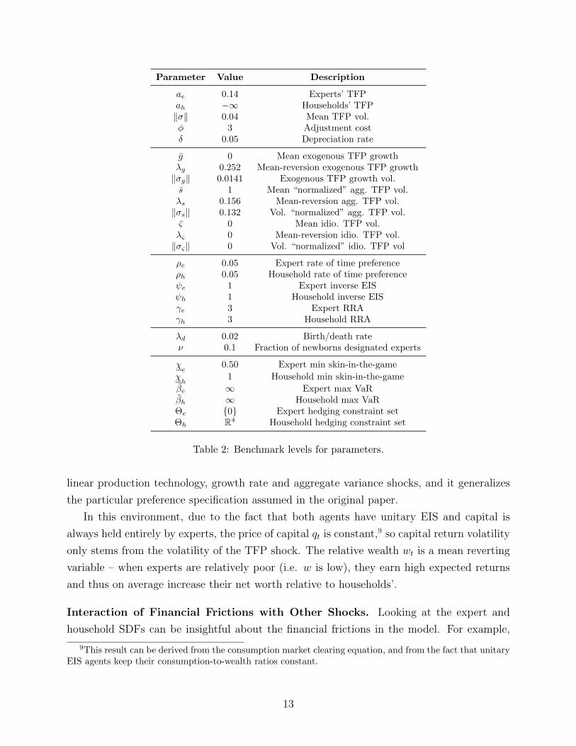
three zero entries and one non-zero entry. See Table 2 for benchmark values.
In our benchmark economic environment, households cannot produce any capital (ah =
−∞), meaning that all the capital in the economy will always be held and operated by
11
Paper Parameters Notes
Basak and Cuoco (1998) ah = −∞, χe
= 1, βe =∞,γh = ψh = 1, γe = ψe,σg = σs = σς = 0
We add production. We alsoadd OLG for stationarity.
He and Krishnamurthy (2013) ah = −∞, χe< 1, βe =∞,
γh = ψh = 1, γe = ψe,σg = σs = σς = 0
We add production. Theirhouseholds also have laborincome.
ρe 0.05 Expert rate of time preferenceρh 0.05 Household rate of time preferenceψe 1 Expert inverse EISψh 1 Household inverse EISγe 3 Expert RRAγh 3 Household RRA
λd 0.02 Birth/death rateν 0.1 Fraction of newborns designated experts
χe
0.50 Expert min skin-in-the-game
χh
1 Household min skin-in-the-game
βe ∞ Expert max VaRβh ∞ Household max VaRΘe {0} Expert hedging constraint setΘh R4 Household hedging constraint set
Table 2: Benchmark levels for parameters.
linear production technology, growth rate and aggregate variance shocks, and it generalizes
the particular preference specification assumed in the original paper.
In this environment, due to the fact that both agents have unitary EIS and capital is
always held entirely by experts, the price of capital qt is constant,9 so capital return volatility
only stems from the volatility of the TFP shock. The relative wealth wt is a mean reverting
variable – when experts are relatively poor (i.e. w is low), they earn high expected returns
and thus on average increase their net worth relative to households’.
Interaction of Financial Frictions with Other Shocks. Looking at the expert and
household SDFs can be insightful about the financial frictions in the model. For example,
9This result can be derived from the consumption market clearing equation, and from the fact that unitaryEIS agents keep their consumption-to-wealth ratios constant.
13
figure 2 shows expert and household risk prices to the TFP and aggregate volatility shocks,
as a function of experts’ wealth share (w) and stochastic variance (s).
Figure 2: Local risk prices πe and πh for the TFP shock (first row) and volatility shock (secondrow). The “single-agent” risk price, from an economy with χ
e= 0, is plotted alongside πe. Expected
growth g is held fixed at g.
As expected, experts’ TFP risk price (top left panel) is falling in their relative wealth and
rising in aggregate volatility. Households’ TFP risk price (top right panel) is approximately
the same as the risk price from a frictionless “single-agent” long-run risks model (e.g., Bansal
and Yaron (2004)), which corresponds to χe
= 0.10
Surprisingly, when their relative wealth is low enough, experts’ volatility risk price (bot-
tom left panel) switches from negative to positive, implying experts can be fond of volatility
shocks. This occurs because the experts’ expected returns on capital are strongly decreasing
and convex in w, inheriting the shape of their TFP risk price (see equation (75) in Appendix
A.5, which shows that TFP risk prices are proportional to w−1). Jensen’s inequality implies
that a positive volatility shock benefits experts. This force outweighs the standard volatility
aversion inherent in these preferences, which shows up in the negative household volatility
risk price (bottom right panel) and the “single-agent” volatility risk price. Importantly, this
insight is only available with the volatility shock introduced in the model: the TFP risk
prices are increasing in volatility for both experts and households, which might suggest a
10In addition, we describe a single-agent long-run risks model, and its analytical solution for the unitaryEIS case, in Appendix D.
14
distaste for volatility in the comparative static sense.
Occasionally-Binding Constraints. Given χe< 1, we might expect equity constraints
to be occasionally-binding, as in He and Krishnamurthy (2013). However, it turns out that
these constraints are always-binding unless experts and households differ in their preferences.
See figure 3, which illustrates this point in a one-dimensional model where w is the only state
variable (i.e., σg = σs = 0 so that g and s are non-stochastic). Thus, implicitly embedded in
some of the “auxiliary assumptions” of He and Krishnamurthy (2013) and other models are
assumptions about heterogeneous preferences.
Figure 3: Expert skin-in-the-game χ (top row) and expert risk prices πe (bottom row). Stationarydensities are shaded in the background. We set σg = σs = 0. In the plots in the right column, wereduce γe from 3 to 1. All other parameters are given in Table 2.
With partial equity issuance (χe< 1), experts’ financing constraint does not bind when
w is sufficiently high. Under symmetric preferences, a non-binding constraint implies local
Sharpe ratios earned by experts and households are equalized. In such an environment, the
wealth share w is locally deterministic, moving purely due to births and deaths, thus exiting
the unconstrained region in finite time. With homogeneous preferences, the ergodic density
of w resides exclusively in the constrained region (top left panel).
On the other hand, with heterogeneous preferences, the ergodic density can include both
the constrained and unconstrained region (top right panel). This results in much more
nonlinearity in experts’ risk prices than in the homogeneous preference case (bottom two
15
panels). Such a situation can materialize because the unconstrained region remains stochastic
(in the sense that σw 6= 0), as is standard in heterogeneous preference models.
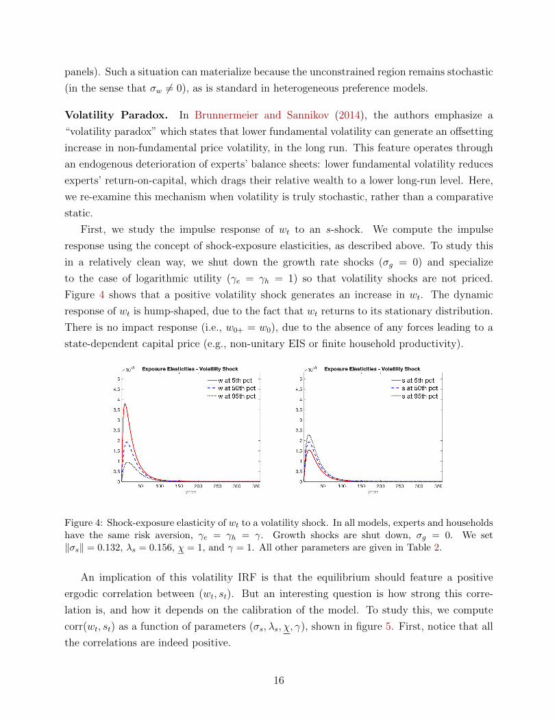
Volatility Paradox. In Brunnermeier and Sannikov (2014), the authors emphasize a
“volatility paradox” which states that lower fundamental volatility can generate an offsetting
increase in non-fundamental price volatility, in the long run. This feature operates through
an endogenous deterioration of experts’ balance sheets: lower fundamental volatility reduces
experts’ return-on-capital, which drags their relative wealth to a lower long-run level. Here,
we re-examine this mechanism when volatility is truly stochastic, rather than a comparative
static.
First, we study the impulse response of wt to an s-shock. We compute the impulse
response using the concept of shock-exposure elasticities, as described above. To study this
in a relatively clean way, we shut down the growth rate shocks (σg = 0) and specialize
to the case of logarithmic utility (γe = γh = 1) so that volatility shocks are not priced.
Figure 4 shows that a positive volatility shock generates an increase in wt. The dynamic
response of wt is hump-shaped, due to the fact that wt returns to its stationary distribution.
There is no impact response (i.e., w0+ = w0), due to the absence of any forces leading to a
state-dependent capital price (e.g., non-unitary EIS or finite household productivity).
Figure 4: Shock-exposure elasticity of wt to a volatility shock. In all models, experts and householdshave the same risk aversion, γe = γh = γ. Growth shocks are shut down, σg = 0. We set‖σs‖ = 0.132, λs = 0.156, χ = 1, and γ = 1. All other parameters are given in Table 2.
An implication of this volatility IRF is that the equilibrium should feature a positive
ergodic correlation between (wt, st). But an interesting question is how strong this corre-
lation is, and how it depends on the calibration of the model. To study this, we compute
corr(wt, st) as a function of parameters (σs, λs, χ, γ), shown in figure 5. First, notice that all
the correlations are indeed positive.
16
Figure 5: Ergodic correlations between(wt, st) for different values of param-eters (σs, λs, χ, γ). In all models, ex-perts and households have the samerisk aversion, γe = γh = γ. Growthshocks are shut down, σg = 0. Withthe exception of the parameter beingvaried, we set ‖σs‖ = 0.132, λs =0.156, χ = 1, and γ = 1. All otherparameters are given in Table 2.
Focusing on the top row shows that, as volatility shocks are larger (higher σs) or more
persistent (lower λs), the ergodic wealth-volatility correlation increases substantially. This
helps explain strength of the comparative static results of Brunnermeier and Sannikov (2014).
The bottom row shows that less equity-issuance (higher χ) or more risk-averse agents (higher
γ) raises the (wt, st) correlation. Intuitively, higher χ or higher γ both scale experts’ risk
compensations, amplifying the effect of a volatility shock.
Are Experts More Productive or Risk-Tolerant? Among many alternatives, we focus
on two competing hypotheses for why subsets of agents (“experts”) take larger amounts of
risk than others. Experts could be more productive managers of capital (ae > ah) or they
could simply be more risk-tolerant (γe < γh). The two models closest to this comparison are
Brunnermeier and Sannikov (2014) versus Garleanu and Panageas (2015).
Figure 6 shows the endogenous capital distribution κ := Ke,t/(Ke,t+Kh,t) as a function of
state variables (w, s), holding fixed g = g. Both models feature regions where κ ∈ (0, 1), but
the heterogeneous productivity model showcases a large part of the state space where experts
hold the entire capital stock. To understand this, consider the Merton portfolio k∗j =µR,j−rγjσR
for agent j. With higher productivity, experts obtain a discretely larger expected return
on capital than households (µR,e > µR,h) than households, so it is possible for households’
desired portfolio to be negative (k∗h < 0), leaving them on their no-shorting constraint. If
experts and households faced the same returns (µR,e = µR,h) but their risk aversions differed
(γe < γh), experts and households would both hold positive quantities of capital but at
different scales (k∗e > k∗h > 0).
In a model with heterogeneous productivity, when households finally do start holding
capital, capital prices fall sharply and risk compensations rise sharply, as seen in figure 7
17
Figure 6: Expert capital share κ as a function of wealth share w and stochastic variance s. Expectedgrowth g is held fixed at g. Left panel has more productive experts (ah = 0.7 < ae = 0.14,γe = γh = 3, ν = 0.01, λd = 0.04). Right panel has more risk-tolerant experts (ah = ae = 0.14,γe = 2 < γh = 8, ν = 0.10, λd = 0.02). Parameters (γe, γh, ν, λd) are chosen such that the long-runmean of wt is approximately the same in the two models. All other parameters are in Table 2.
(left panel). In contrast, a model with heterogeneous preferences features much smoother
and more gradual risk price dynamics. Importantly, this comparison is made holding the
wealth distribution relatively fixed across the two models (this is accomplished by varying
parameters (γe, γh, ν, λd) to adjust the densities of wt). In future analyses, we would like
to experiment with imposing additional observational constraints in our model comparisons
(e.g., similar average risk prices). Imposing observational constraints can impose strong
discipline on the models in searching for distinguishing features.
These observed differences between experts’ risk prices also show up in the shock-price
elasticities of these models. The bottom row of figure 8 illustrates the term structure of
experts’ TFP risk prices. When experts’ relative wealth is moderate (e.g., wt at its median),
the term structures between the models are similar. When experts are distressed (e.g., wt at
a low percentile), they look different: in the heterogeneous productivity model, the level of
the term structure rises dramatically, and it becomes more negatively-sloped.
The top row shows that risk exposures in the heterogeneous productivity model are also
higher when wt is low, whereas they are invariant to wt in the heterogeneous risk aversion
model. To generate a closer link between the models on this dimension, we would need to
calibrate non-unitary EIS in the heterogeneous risk aversion model, which we leave for a
future iteration.
Another interesting difference between these models is embedded in experts’ perception of
18
Figure 7: Experts’ TFP risk prices πe in models with heterogeneous productivity versus hetero-geneous risk aversion. Stationary densities are shaded in the background. Expected growth g isheld fixed at g. Left panel has more productive experts (ah = 0.7 < ae = 0.14, γe = γh = 3,ν = 0.01, λd = 0.04). Right panel has more risk-tolerant experts (ah = ae = 0.14, γe = 2 < γh = 8,ν = 0.10, λd = 0.02). Parameters (γe, γh, ν, λd) are chosen such that the long-run mean of wt isapproximately the same in the two models. All other parameters are in Table 2.
Figure 8: Shock-exposure and -price elasticities of aggregate consumption Ct to the TFP shock.Expected growth g is held fixed at g. Left column has more productive experts (ah = 0.7 <ae = 0.14, γe = γh = 3, ν = 0.01, λd = 0.04). Right column has more risk-tolerant experts(ah = ae = 0.14, γe = 2 < γh = 8, ν = 0.10, λd = 0.02). Parameters (γe, γh, ν, λd) are chosen suchthat the long-run mean of wt is approximately the same in the two models. All other parametersare in Table 2.
volatility shocks. Figure 9 shows shock-exposure and shock-price elasticities to a st-shock. In
normal times (e.g., wt at its median), the two models both produce similar volatility shock-
19
exposure and shock-price elasticities. The positive sign and shape of the volatility shock-
exposure elasticity are standard in long-run risk models: higher volatility of log consumption
leads to higher future expected consumption through a Jensen effect. The positive sign of
the volatility shock-price elasticity is due to the possibility of experts’ demanding a positive
volatility risk price, as in the discussion surrounding figure 2.
In bad times (e.g., wt at its 5th percentile), the sign of both the exposure and price
elasticities flip dramatically in the heterogeneous productivity model (left column). In such
times, households are now holding capital, and a positive volatility shock further increases
their desire to hold capital (this can also be seen in the left panel of figure 6). This leads
a strong decline in capital prices, output, and consumption. Without these forces, experts
liked volatility shocks, because their risk prices were strongly convex in wt. With capital
reallocation, πe is less strongly convex in wt, attenuating this force. More importantly, with
an expected decline in aggregate consumption, there is a direct negative impact of a positive
volatility shock.
Figure 9: Shock-exposure and -price elasticities of aggregate consumption to the volatility shock.Expected growth g is held fixed at g. Left column has more productive experts (ah = 0.7 <ae = 0.14, γe = γh = 3, ν = 0.01, λd = 0.04). Right column has more risk-tolerant experts(ah = ae = 0.14, γe = 2 < γh = 8, ν = 0.10, λd = 0.02). Parameters (γe, γh, ν, λd) are chosen suchthat the long-run mean of wt is approximately the same in the two models. All other parametersare in Table 2.
20
Differential Consumption Dynamics. Because of financial frictions, the dynamics of
experts’ and households’ consumptions can be very different. Figure 10 plots shock-exposure
elasticities for Ce and Ch in the previous heterogeneous productivity model. Again, these
can be thought of as nonlinear IRFs.
Figure 10: Shock-exposure elasticities for expert consumption Ce (left column) and householdconsumption Ch (right column). Expected growth g is held fixed at g. The parameters for thismodel coincide with the heterogeneous productivity model (ah = 0.7 < ae = 0.14, γe = γh = 3,ν = 0.01, λd = 0.04). All other parameters are in Table 2.
Because experts have leverage, their consumption responds much stronger to a positive
TFP shock (top row). As w falls, expert leverage rises, so their consumption is accordingly
more sensitive to a TFP shock. The growth rate shocks are shared perfectly in this economy,
in the sense that Ce and Ch respond identically to a g-shock (middle row). This occurs
because of the unitary EIS assumption of this model, something we plan to relax in the
future. Finally, volatility shocks generate highly asymmetric responses between experts and
households. In normal times (e.g., w at its median), one can see, by comparing the responses
of Ce and Ch, that the response of w := Ne/(Ne+Nh) ≡ Ce/(Ce+Ch) is qualitatively similar
21
to the IRFs in figure 4. As before, higher volatility improves experts’ investment opportunities
relative to households, which improves their future consumption. In bad times (e.g., w at
its 5th percentile), an increase in volatility lowers capital prices, which predominantly affects
experts, so their consumption drops in the short run.
5 Conclusion
In this paper, we develop a general macroeconomic model with financial frictions that en-
compasses many recent papers in the literature. By varying parameters in the model, we
compare implications of various financial frictions, preference constellations, and exogenous
state variables. By introducing a model more general than those in the literature, we are
also able to explore interactions between features of disparate models from the macro-finance
literature. So far, we have made a subset of the comparisons we are interested in.
Readers can experiment with some of the parameter constellations we have solved by vis-
return to “inside equity” whereas (1−χ)π ·σR represents experts’ payout to “outside equity”
held by households. Simply by accounting, these sum to the excess return on assets, and ∆e
can thus be interpreted as the bonus return per unit of inside equity, of which there are χ
units.
Finally, we substitute the optimal choices (32) and (36) back into the HJB equations.
When doing this substitution, we use the fact that µnh = r + σnh · π + βh∆h and that
µne = r + βe (∆e + σR · π). We also use the fact that σnh = βh√ς for households, and that
σne = βeσR and that σne = βe√ς for experts. For households, we obtain:
0 =ψh
1− ψhρ1/ψh
h ξ1−1/ψh
h − ρh1− ψh
+ r +1
2γh
(‖π‖2 + (γhβh
√ς)2)
+[µX +
1− γhγh
σXπ]· ∂X ln ξh
+1
2
[tr(σ′X∂XX′ ln ξhσX) +
1− γhγh
‖σ′X∂X ln ξh‖2]
(38)
Without idiosyncratic capital quality shocks (i.e. when ς = 0), the term γhβh√ς disappears
and we obtain the complete market, recursive preference HJB equation. For experts:
0 =ψe
1− ψeρ1/ψee ξ1−1/ψe
e − ρe1− ψe
+ r +1
2γe
(∆e + π · σR)2
‖σR‖2 + ς+[µX +
1− γeγe
(∆e + π · σR‖σR‖2 + ς
)σXσR
]· ∂X ln ξe
+1
2
[tr(σ′X∂XX′ ln ξeσX) +
1− γeγe
(σ′X∂X ln ξe)′[γeId + (1− γe)
σRσ′R
‖σR‖2 + ς
]σ′X∂X ln ξe
](39)
In the above, Id is the d × d identity matrix. Aside from the idiosyncratic risk that house-
30
holds are forced to bear, their HJB equation is a standard equation for a complete-markets
investor with recursive preferences. Experts HJB equation additionally has effects of finan-
cial frictions, including the presence of the bonus risk premium ∆e and the inability to hedge
aggregate risks associated with (g, s, ς). Boundary conditions for (38) and (39) will be dis-
cussed below. Note also that the same PDEs hold for unitary IES investors, except that the
term ψ1−ψρ
1/ψξ1−1/ψ − ρ1−ψ is replaced by ρ (ln ρ− ln ξ)− ρ.11
A.3 Solving for equilibrium dynamics
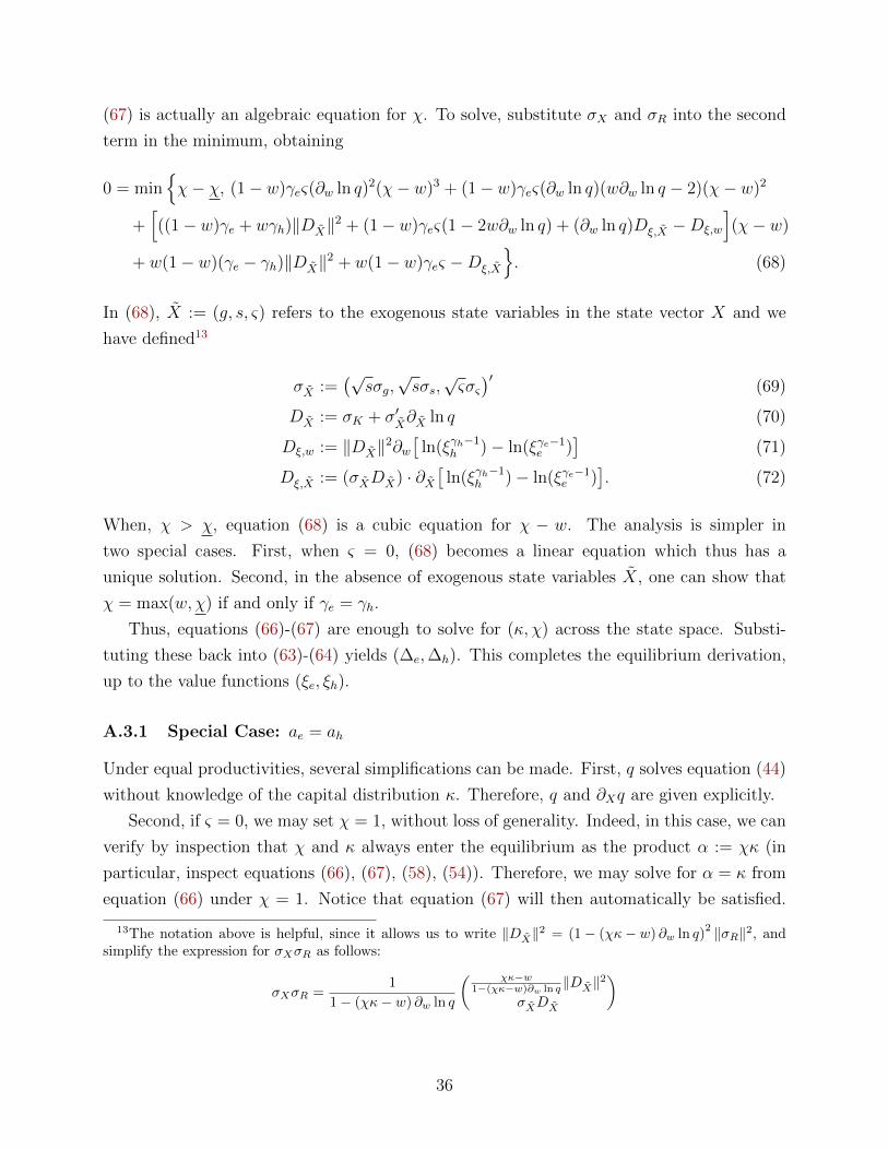
To characterize equilibrium, we must determine (i) q and its dynamics as a function of X;
(ii) r, π, ∆e and ∆h as a function of X; and (iii) the dynamics of X. Because of the
constraints χ ≥ χ and kh ≥ 0, the state space must be partitioned into regions in which
various constellations of constraints bind. To do this, define κt := Ke,tKt
to be the fraction
of capital managed by experts. There are 3 cases to consider, by considering the Euler
inequalities (31) and (35) for households and experts:12
• κ = 1 and χ > χ – In this case, all the capital is managed by experts, who are wealthy
enough that their skin-in-the-game constraint is not binding. In this region, we have:
µR,e − r = π · σR > µR,h − r
• κ = 1 and χ = χ – In this case, all the capital is managed by experts, but their
skin-in-the-game constraint is now binding. In this region, we have:
µR,e − r > π · σR > µR,h − r
• κ < 1 and χ = χ – In this case, experts’ net worth, compared to the aggregate wealth in
the economy, is too small, experts’ risk-bearing capacity is low and some of the capital
has to be held by household, whose productivity is lower than the experts’. In this
region, we have:
µR,e − r > µR,h − r ≥ π · σR11Note that this formula can easily be obtained using L’Hopital’s rule, noticing that:
limψ→1
ψρ1/ψξ1−1/ψ
1− ψ− ρ
1− ψ= ρ (ln ρ− ln ξ)− ρ
12This applies when ae > ah holds. If so, the case χ > χ and κ < 1 can be ruled out. Indeed, in such acase, agents’ Euler equations (31) and (35) imply that µR,e − r = µR,h − r, which contradicts (7). We needto consider this case when ae = ah, which is treated in subsection A.3.1.
31
In the absence of idiosyncratic capital quality shocks (i.e. when ς = 0), the last
inequality is actually an equality – i.e. µR,h − r = π · σR. In other words, since
households have no constraints, their expected return on capital must be equal to the
market compensation for aggregate risk.
Combining these conditions with the definitions of ∆e and ∆h in (37) and (34), we completely
summarize the constraints with the following complementary slackness conditions:
0 = min(1− κ,∆+h −∆h) (40)
0 = min(χ− χ,∆e) (41)
0 = (1− κ)(χ− χ)(ae − ah). (42)
We will use these conditions to determine where constraints bind.
Before considering the state space partitions coming from constraints, we make use of
some equilibrium conditions that apply across the state space. First, the goods market
clearing condition (17) implies
q(1− w)ρ1/ψhh ξ
1−1/ψhh + qwρ1/ψe
e ξ1−1/ψee = (1− κ)ah + κae − Φ(ι(q)). (43)
Equation (43) relates q and κ to the state variables, conditional on ξh and ξe. Notice that
the left-hand-side (as a function of q) is strictly increasing, while the right-hand-side is
strictly decreasing, yielding a unique q that satisfies the goods market clearing condition
above. Notice also that in the unitary IES case, when all the capital in the economy is held
by experts (i.e. κ = 1), the price of capital is constant, simply equal to the ratio of (a)
the dividend yield ae − Φ (ι(q)) divided by (b) a weighted average rate of time preference
wρe + (1 − w)ρh. With Φ(x) = φ−1[exp(φx) − 1], we use (28) in equation (43) to get the
following special case:
q =(1− κ)ah + κae + 1/φ
(1− w)ρ1/ψhh ξ
1−1/ψhh + wρ
1/ψee ξ
1−1/ψee + 1/φ
(44)
Next, the dynamics of aggregate capital are derived from time-differentiating the capital
market clearing condition (18), using the laws of motion for individual capital stocks in (1),
the common investment rate defined by (26), and the law of large numbers:
dKt
Kt
= µK,tdt+ σK,t · dZt (45)
µK,t := gt + ι(qt)− δ. (46)
32
To determine the dynamics of the wealth share wt, combine agents’ net worth dynamics
with their portfolio choices (i.e., combine (13) with (32) for households and with (36) for
experts), and the law of large numbers, to obtain evolutions for aggregate household and
expert net worths Nh,t :=∫Jhnj,tdj and Ne,t :=
∫Je nj,tdj:
dNh,t
Nh,t
=[rt − ρ1/ψh
h ξ1−1/ψhh − λd + σnh,t · πt + βh,t∆h,t +
(1− ν)λd1− wt
]dt+ σnh,t · dZt (47)
dNe,t
Ne,t
=[rt − ρ1/ψe
e ξ1−1/ψee − λd + σne,t · πt + βe,t∆e,t +
νλdwt
]dt+ σne,t · dZt. (48)
The terms containing λd represent contributions from OLG. Using risk choices (32) and (36),
combined with equity market clearing (19) and the definitions of w and κ, we have
σnh =1− χκ1− w
σR (49)
σne =χκ
wσR. (50)
By Ito’s formula, the wealth share w = NeNe+Nh
evolves as
dw = w(1− w)[dNe
Ne
− dNh
Nh
]− w(1− w)
[wd[Ne]
N2e
− (1− w)d[Nh]
N2h
+ (1− 2w)d[Ne, Nh]
NeNh
].
Using (47)-(48) and (49)-(50), and making several simplifications, the result is
µw = w(1− w)[ρ
1/ψhh ξ
1−1/ψhh − ρ1/ψe
e ξ1−1/ψee + βe∆e − βh∆h
]+ (χκ− w)σR · (π − σR) + λd(ν − w) (51)
σw = (χκ− w)σR. (52)
Together with the exogenous dynamics in (2), (3), and (4), the endogenous dynamics in
(51)-(52) fully describe the dynamics of Xt, i.e.,
µX =(µw, λg(g − g), λs(s− s), λς(ς − ς)
)′(53)
σX =(σw,√sσg,
√sσs,√ςσς
)′. (54)
By Ito’s formula, the dynamics of qt are
dq(Xt) =[µX(Xt) · ∂Xq(Xt) +
1
2tr(σX(Xt)
′∂XX′q(Xt)σX(Xt))]dt
+[σX(Xt)
′∂Xq(Xt)]· dZt. (55)
33
Since µX does not depend directly on µq, the drift term may be obtained simply from the
Ito’s formula expansion:
µq =1
q
[µX · ∂Xq +
1
2tr(σ′X∂XX′qσX)
]. (56)
On the other hand, σX depends on σq, constituting a two-way feedback loop. We can solve
this loop by substituting (54) into σq in (55), using σR = σK + σq:
σq =(χκ− w) (∂w ln q)
√sσ + (∂g ln q)
√sσg + (∂s ln q)
√sσs + (∂ς ln q)
√ςσς
1− (χκ− w)∂w ln q(57)
This is a d × 1 equation. Conditional on knowing χ and κ, if we know the price function q
across the state space, we know the capital price volatility vector σq, as well as the wealth
share volatility vector σw. Note that this generates capital return volatility equal to
σR =
√sσ + (∂g ln q)
√sσg + (∂s ln q)
√sσs + (∂ς ln q)
√ςσς
1− (χκ− w)∂w ln q. (58)
Finally, we solve for the stochastic discount factor coefficients (r, π). Time-differentiate
the bond market clearing condition (20), using the evolutions of Nh and Ne in (47) and (48),
and K in (45). By equating the drift terms:
r + (1− w)(σnh · π + βh∆h − ρ1/ψh
h ξ1−1/ψhh
)+ w
(σne · π + βe∆e − ρ1/ψe
e ξ1−1/ψee
)= µq + µK + σK · σq (59)
By equating the diffusion terms:
(1− w)σnh + wσne = σR. (60)
To solve for r, substitute (60) into (59) and rearrange:
Thus, the original PDE (79) is the stationary solution to the augmented PDE (80), i.e.,
∂tf = 0 holds in (80). The following method solves (80) iteratively until ∂tf ≈ 0.
Step 0: Initialization. Form a guess for φ0(x) := f(x, T ), which is the terminal condition.
Step k: Discretization, Linearization, Iteration. Generate a grid of time points {T, T −∆t, . . . }and a grid of space points X . Given a candidate function φk(x) for f(x, T − k∆t)
restricted to X , compute finite difference approximations to all derivatives. The time-
derivative is approximated with the backward difference
φk(x)− φk+1(x)
∆t≈ ∂tf(x, T − k∆t)
Denote the finite-difference approximations of the spatial derivatives by
∂xφk(x) ≈ ∂xf(x, T − k∆t)
∂xx′φk(x) ≈ ∂xx′f(x, T − k∆t).
Both ∂x and ∂xx′ are always computed using central differences, except at the boundaries
of X , where they are computed via central differences at the nearest interior point.
Using these approximations everywhere in (80), we can solve for φk+1 given φk via
Define q according to equation (44) with κ = 1. Using q and its derivatives
in place of q, as well as κ = 1 and y(l), compute A0, A1, A2, A3. Solve the
equation F (w, χ) = 0 for χ at each w. If ς = 0, then this equation is linear
and has a unique solution; otherwise, use any nonlinear solver with initial
guess χ = χ(l). Denote the solution by χ. If χ ≥ χ, set χ(l+1) = χ. Otherwise,
there are two cases:
• If F (w, χ) > 0, then set χ(l+1) = χ.
• If F (w, χ) < 0, then set χ(l+1) = +∞ (or some very large number).
iv. Use equation (63) to solve for ∆(l+1)e , then set ∆
(l+1)h by (64). Use κ(l+1) and
χ(l+1) but y(l) for everything else in this step.
v. Set q(l+1) by equation (44), using κ(l+1) and (ξ(n)e , ξ
(n)h ).
(c) Iterate on (b). When ‖κ(l+1) − κ(l)‖+ ‖χ(l+1) − χ(l)‖ is small, stop iterating.
(d) Put y(n) = y(l).
2. Outer loop: update value functions using PDEs. Update ξ(n+1)e , ξ
(n+1)h by iterat-
ing one time-step in their the PDEs (39) and (38). This involves augmenting the PDEs
with fictitious time derivatives, or “false transients”, as discussed in Appendix B.1. If
ψe = 1 or ψh = 1, replace ψ1−ψρ
1/ψξ1−1/ψ− ρ1−ψ by ρ (ln ρ− ln ξ)−ρ. All the coefficients
in the PDEs are computed using step-n objects.
B.3 Solving Linear Systems
The following algorithm summarizes our numerical solution of PDEs (39) and (38) for
ζk∈(e,h) := ln ξk∈(e,h), based on Appendixes B.1 and B.2.
42
Initialization: Start with guess functions ζ0k∈(e,h).
while supx‖ζtk(x)− ζt−1
k (x)‖ > ε or t = 0 do
(0) Update the iterator t = t+ 1;
(1) Refresh equilibrium quantities which are functions of ζt−1k ;
(2) Update the PDE coefficients, which depend on the updated equilibrium
quantities and ζt−1k . In this process, treat the non-linear terms of ζk as if
ζk = ζt−1k . Therefore, the only terms left unknown are linear terms of ζk;
(3) Construct the linear systems Atkζtk = btk as the finite difference representation
of the linear PDEs from (2);
(4) Solve Atkζtk = btk for ζtk using some linear system solver ;
end
When the algorithm finishes, we take the solutions from the final iteration in the while
loop as the solutions to the PDEs.
To do step (4), which involves solving Atkζ=k b
tk, we have taken two distinct approaches. As
a first option, we have leveraged the high-performance computing package Pardiso15 in C++
to perform an LU decomposition of the matrix Atk. In what follows, we call this, including
the use of the Pardiso package, the “LU approach.” This has two drawbacks. First, in each
iteration t, we need to perform LU decomposition for a brand new matrix, as the coefficients
of the PDEs get updated in each iteration. Second, finding the LU decomposition of Atkis costly, because of its dimensionality (it encodes a 4-dimensional finite difference scheme,
which is large, even considering its sparsity).
As a second option, we have solved Atkζ=k b
tk using the conjugate gradient method, which
is one example of a Krylov subspace method.
Conjugate Gradient Method. For an n × n symmetric positive definite matrix A, the
conjugate gradient (CG) method solves the linear system Ax = b by minimizing the quadratic
form:
min f(x) =1
2xTAx− xT b
The first order condition of this minimization problem is
∂xf(x) = Ax− b = 0
Therefore, if A is positive definite, solving the linear system is equivalent to finding the min-
Figure 11: Time Performance for CG vs LU Decomposition (implemented by Pardiso)
Test: Role of Time Step. The time step (∆t), used in iterating on the PDEs for ζk,
is an important numerical parameter. With CG, ∆t captures a trade-off between speed of
convergence in the VFI “outer loop” versus the CG “inner loop”. A higher ∆t reduces the
number of value function iterations (VFI) for {ζtk} to converge in the outer loop. On the
other hand, higher ∆t increases the number of CG inner loop iterations, as the initial guesses
for ζkt are less accurate. Figure 12 illustrates this trade-off.
Although the highest ∆t = 0.5 requires significantly more time in the beginning, it quickly
finds the right solution and the number of inner loop iterations decreases very fast (perhaps
aided by the smart guess approach). With ∆t = 0.01, the algorithm requires significantly
more outer loop iterations and the total time taken is longer. This test shows that, in this
case, reducing the number of iterations (higher ∆t) dominates very accurate guesses at all
iterations (lower ∆t).
45
(a) Time taken per outer loop iteration (b) Total time taken to solve model
Figure 12: Role of Time Step
46
C Shock Elasticities
Some recent papers have characterized shock-exposure and shock-price elasticities, arguing
that they is an alternative and useful way to depict asset prices in dynamic models.16 The
following discussion provides a short overview.
Setup and Definition. In the class of models we consider, there will always be a n-
dimensional state variable Xt following a diffusion
dXt = µX(Xt)dt+ σX(Xt)dZt (84)
There will also be an equilibrium stochastic discount factor St, which follows
d logSt = µS(Xt)dt+ σS(Xt) · dZt. (85)
Finally, any cash flow process {Gt} can be constructed from the Markov state {Xt} as
d logGt = µG(Xt)dt+ σG(Xt) · dZt. (86)
Assume this cash flow {Gt} is priced by the SDF {St}. Given these processes, we can
construct shock elasticities as follows. Define {Mt} be a logarithmic process analogous to
{Gt} and {St}:d logMt = µM(Xt)dt+ σM(Xt) · dZt.
Define the exponential martingale Hνs := exp
( ∫ s0ν(Xu)·dZu− 1
2
∫ s0|ν(Xu)|2du
), where ν(x) ∈
Rd and ‖ν(x)‖ = 1. Then, define the shock elasticity for process M at horizon t to be
εM(t, x) := lims↘0
1
slogE
[(Mt
M0
)Hνs | X0 = x
], (87)
By Girsanov’s theorem, Hνs acts to alter the distribution of shocks to which M is exposed
between times [0, s]. By altering the distribution of shocks, εM(t, x) measures a type of
non-linear impulse response, tracing the effect of this altered distribution over a horizon t.17
Interpretation as an Increase in Exposure. Equivalently, Hνs acts to perturb the shock
16See Borovicka et al. (2011), Hansen (2012), Hansen (2013). An accessible review treatment is providedin the handbook chapter Borovicka and Hansen (2016).
17This logic is made precise in Borovicka, Hansen, and Scheinkman (2014).
47
exposure of M near time 0. To see this equivalence, look at
logMt
M0
Hνs =
∫ s
0
[µM(Xu)−
1
2ν(Xu)
]du+
∫ s
0
[σM(Xu) + ν(Xu)
]· dZu
+
∫ t
s
µM(Xu)du+
∫ t
s
σM(Xu) · dZu.
On the interval [0, s], MHν has perturbed exposure σM(Xu) + ν(Xu) to the Brownian shock
dZu. For example, when M = G, we can think of MtHνs as a perturbed cash flow, which has
a vector ν of additional shock exposures near time 0. Then the function εM(t, x) traces out
the expected effect of this instantaneous increase in shock exposure over a horizon t. The
fact that ‖ν(x)‖ = 1 justifies the use of the term “elasticity”. We will typically take ν to be
a coordinate vector to interpret εM as the response of M to a particular shock.
Asset-Pricing. The shock-exposure elasticity is defined by εG and the shock-price elasticity
is defined by εG − εSG. The shock-exposure elasticity answers the question: how sensitive is
the expected cash flow Gt to an increase in its risk exposure at time 0?
The shock-price elasticity is slightly more nuanced. Because E[StGt] is the scaled price of
the cash flow Gt, and GHν is the perturbed cash flow, εSG is the sensitivity of the price to
an increase in the risk exposure of Gt. Since log(E[Gt]E[St]/E[StGt]) is a log expected excess
return, shock-price elasticities answer the question: how much are expected excess returns
required to increase with an increase in the exposure of Gt to a particular shock at time 0?
It is in units of Sharpe ratios, or risk prices, because Hν delivers a unit standard deviation
increase in the risk exposure of Gt. Thus, the shock-price elasticity is often interpreted as a
term structure of risk prices.
Computation. The shock elasticities are computed by applying Malliavin calculus, which
is beyond the scope of this Appendix. The result is (see the papers cited above)
εM(t, x) = ν(x) ·{σM(x) + σX(x) · ∂
∂xlogE
[(Mt
M0
)| X0 = x
]}. (88)
To compute each of the conditional expectations in (88) numerically, we solve a PDE de-
rived as follows. Define fM(t, x) := E[Mt
M0fM(0, Xt) | X0 = x]. Then, using the law of iterated
expectations, followed by the definition of fM , we have fM(t, x) = E[Mu
M0E[Mt
MufM(0, Xt) | Xu] |
X0 = x] = E[Mu
M0fM(t−u,Xu) | X0 = x]. Hence, {MtfM(T − t,Xt)}t∈[0,T ] is a martingale and
must have zero drift. Applying Ito’s formula gives a PDE for fM in (t, x), i.e.,
0 = −∂fM∂t
+(µM +
1
2‖σM‖2
)fM +
(µX + σM · σX
)∂fM∂x
+1
2‖σX‖2∂
2fM∂x2
. (89)
48
The initial condition is fM(0, x) ≡ 1, which allows us to recover the desired conditional
expectation. We obtain εM(t, x) by numerically differentiating fM(t, x) and substituting it
into (88). Note also that the term structure of interest rates can be obtained by solving PDE
(89) with M = S and taking r(t, x) := −1t
log fS(t, x).
We solve PDE (89) subject to boundary conditions at the boundaries of the domain of
Xt. These typically depend on the nature of the model, i.e., (µX , σX), as well as the process
(µM , σM). In models we consider, boundaries are inaccessible by Xt, so we impose zero first
derivatives at those boundaries.
Alternative Shock Elasticities. There is also a second type of shock elasticity, which
differs conceptually from the first type. While εM(t, x) measures the expected response of
Mt to a shock at time 0, we could also compute the expected response of Mt to a shock at
the same time t. Denote this elasticity by εM(t, x), which is computed by replacing Hνs in
(87) by Hνs := exp(
∫ t+st
ν(Xu) · dZu − 12
∫ t+st|ν(Xu)|2du). Because Hν is also a martingale
perturbation, this alternative shock elasticity shares some interpretations with the benchmark
shock elasticities, except the shock is presumed to impact M at some future time.
It turns out that we can compute this alternative shock elasticity via
εM(t, x) = ν(x) ·E[Mt
M0σM(Xt) | X0 = x]
E[Mt
M0| X0 = x]
, (90)
which requires solving the PDE (89) twice with initial conditions fM(0, x) ≡ σM(x) and
fM(0, x) ≡ 1, then taking the ratio to get εM .
49
D Long Run Risk Model with Production
In this case, the aggregate state vector Xt is simply (gt, st). Thus, the drift vector µX(X) and
the volatility matrix σX(X) are exogenously specified. We assume complete markets. We
show that if we know π(X), r(X), we can compute the (scaled) value function ξ(X). Indeed,
the PDE that ξ solves is the following:
0 =ψ
1− ψρ1/ψξ1−1/ψ − ρ
1− ψ+ r +
‖π‖2
2γ+[µX +
1− γγ
σXπ]· ∂X ln ξ
+1
2
[tr(σ′X∂XX′ ln ξσX) +
1− γγ‖σ′X∂X ln ξ‖2
](91)
We then show that if we know ξ(X), we can compute all the equilibrium objects π(X), r(X), q(X).
First, the consumption market clearing gives us q:
ρ1/ψξ1−1/ψ =a− Φ (ι(q))
q
In the above, ι(q) = (Φ′)−1(q). Using our specification for the adjustment cost function Φ,
we obtain:
q =a+ 1/φ
ρ1/ψξ1−1/ψ + 1/φ
Second, equalizing the drifts and volatilities of qK = N leads to:
µq + µK + σq · σK = µn − c
σq + σK = σn
Remember that we have:
µn = r + σn · π
σn =π
γ+
1− γγ
σ′X∂X ln ξ
c = ρ1/ψξ1−1/ψ
Finally, remember that:
µK = ι(q) + g − δ
σK =√sσ
50
Matching the volatility terms leads to:
σ′X∂X ln q +√sσ =
π
γ+
1− γγ
σ′X∂X ln ξ
⇒ π = γσ′X∂X ln q + (γ − 1)σ′X∂X ln ξ + γ√sσ
Matching the drift terms leads to the following expression for r:
r = µX · ∂X ln q +1
2
[tr (σ′X∂XX′ ln qσX) + |σ′X∂X ln q|2
]+ ι(q) + g − δ +
√sσ · (σ′X∂X ln q)
− ‖π‖2
γ+γ − 1
γπ · (σ′X∂X ln ξ) + ρ1/ψξ1−1/ψ
Reinjecting into (91), it can then be verified that the PDE that ξ satisfies is the following:
0 =ρ1/ψξ1−1/ψ − ρ
1− ψ+[µX + (1− γ)
√sσσX
]· ∂X ln (qξ) +
1
2tr (σ′X∂XX′ ln (qξ)σX)
+1− γ
2‖σ′X∂X ln (qξ) ‖2 + ι(q) + g − δ − γ
2‖σ‖2s
In the unitary IES case, the capital price is constant, equal to q = a+1/φρ+1/φ
. The risk price and
risk free rates take the familiar form:
π = (γ − 1)σ′X∂X ln ξ + γ√sσ
r = ρ+ ι(q) + g − δ −√sσ · π
Note that in that case, the PDE satisfied by ξ simplifies to:
ρ ln ρ− ρ ln ξ + ι(q) + g − δ − γ
2‖σ‖2s+
[µX + (1− γ)
√sσXσ
]· ∂X ln ξ
+1
2tr(σ′X∂XX′ ln ξσX) +
1− γ2‖σ′X∂X ln ξ‖2 = 0
Remember that the drift vector and volatility matrix take the following form:
µX =
(λg(g − g)
λs(s− s)
)(92)
σX =√s
(σ′g
σ′s
)(93)
51
Then guess that ln ξ(g, s) = α0 + αgg + αss, reinject to find 3 equations in 3 unknown
α0, αg, αs:
ρ ln ρ− ρα0 + ι(q)− δ + λggαg + λssαs = 0
−ραg + 1− λgαg = 0
−ραs −γ
2‖σ‖2 + (1− γ)σ · [αgσg + αsσs]− λsαs +
1− γ2‖αgσg + αsσs‖2 = 0
When γ 6= 1, αs is the root of a quadratic equation:
1− γ2‖σs‖2α2
s + [(1− γ)σs · (αgσg + σ)− (ρ+ λs)]αs +1− γ
2‖αgσg + σ‖2 − ‖σ‖
2
2= 0
We are interested in the root αs of this quadratic equation such that the implied long-run
risk-neutral measure induces stochastic stability. As argued by Hansen and Scheinkman
(2009), this is the right-most zero of the quadratic equation above. We obtain the following:
αg =1
ρ+ λg(94)
αs =
[(γ − 1)σs · (αgσg + σ) + ρ+ λs
(γ − 1)‖σs‖2
][√√√√1−‖αgσg + σ‖2 − ‖σ‖2
(γ−1)( (γ−1)σs·(αgσg+σ)+ρ+λs(γ−1)‖σs‖
)2 − 1
](95)
α0 =ρ ln ρ+ ι(q)− δ + λggαg + λssαs
ρ(96)
If γ = 1, the coefficient αs is instead equal to αs = −‖σ‖22(ρ+λs)
. In this particular model set-up,
risk-prices and risk-free rates take the following form:
π =√s [(γ − 1) (αgσg + αsσs) + γσ] (97)
r = ρ+ ι(q) + g − δ − s[γ‖σ‖2 + (γ − 1)σ · (αgσg + αsσs)
](98)
The expected excess return on capital is then the following:
Et [dRt − rtdt] = σR,t · πt= st [(γ − 1) (αgσg + αsσs) + γσ] · σ
52
With ψ = 1, the consumption-capital ratio is constant, so consumption dynamics d logCt =
µC,tdt+ σC,t · dZt are given by
µC = ι(q)− δ + g − 1
2s‖σ‖2 := µC0 + µCg(g − g) + µCs(s− s)
σC =√sσ :=
√sσC
Similarly, if St is the stochastic discount factor, d logSt = µS,tdt+ σS,t · dZt are given by
µS = −r − 1
2‖π‖2 := µS0 + µSg(g − g) + µSs(s− s)
σS = −π :=√sσS
In the above, we have introduced the constants µS0 , µC0 , µSg , µCg , µSs , µCs , σS: