Comparing brains and DNNs: Methods and findings

Martin Hebart

Laboratory of Brain and CognitionNational Institute of Mental Health

Bethesda, MD, USA

What information does a neuron represent?

BrainImage

What information does a neuron represent?

DNN BrainImage

Ponce et al, 2019, NeuronWalker et al, 2018, bioRxiv Bashivan et al, 2019, Science

Mouse V1 Monkey V4 Monkey IT

Overview

Comparing brains and DNNs: Overview

Methods and findings for comparing brains and DNNs

Practical considerations

Disclaimer / comments

• Presentation offers only incomplete overview

• Focus on methods and results, less interpretation

• More human data, more similarity-based methods

• Strong focus on vision

Comparing brains and DNNs: Overview

2. Extract

activation

estimate for

condition

3. Vectorize

(i.e. flatten)

pattern

1. Identify pattern

(e.g. region of

interest)

Brain (e.g. fMRI)

…

0.1 0.8

2.0

0.80.6

0.6

0.1

0.8

0.5

0.8

0.8

1.2

1.2

0.6 1.2

1.20.14. Get pattern for

all conditions

Comparing brains and DNNs: Overview

2. Extract

activation

estimate for

condition

3. Vectorize

(i.e. flatten)

pattern

1. Identify pattern

(e.g. region of

interest)

Brain (e.g. fMRI) DNN

…

1. Choose DNN

architecture and

layer

2. Push image

through DNN and

extract activation

at layer

3. Vectorize

(i.e. flatten)

pattern…

4. Get pattern for

all conditions

4. Get pattern for

all conditions

Comparing brains and DNNs: Overview

Brain (e.g. fMRI)

… …

DNN

n conditions

n conditions

p v

oxels

q u

nit

s

Comparing brains and DNNs: Overview

Brain (e.g. fMRI) DNN

p v

oxels

q u

nit

s

n conditions

Goal: Relate to

each other

n conditions

Overview of methods relating DNNs and brains

Decoding: h: Y X

Encoding: g: X Y

Y: Measurement (brain data)

S: Stimuli

X: Model (stimulus feature representation)

X = f(S)

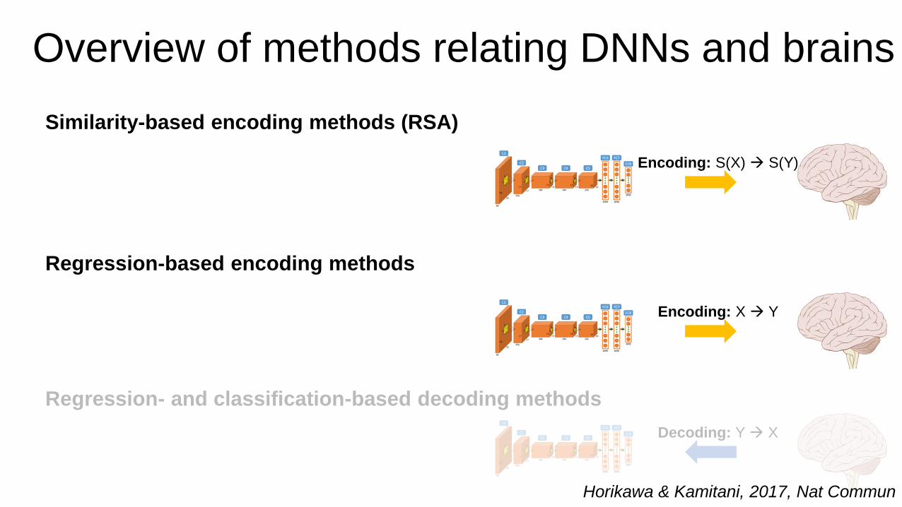
Overview of methods relating DNNs and brains

Encoding: S(X) S(Y)

Similarity-based encoding methods (RSA)

Regression-based encoding methods

Regression- and classification-based decoding methods

Decoding: Y X

Encoding: X Y

Horikawa & Kamitani, 2017, Nat Commun

Similarity-based encoding methods

Encoding: S(X) S(Y)

Vanilla representational similarity analysisp

vo

xels

q u

nit

s

n conditions n c

on

dit

ion

s

Brain (e.g. fMRI betas)

DNN layer activationsn conditions

1 - Pearson R

n conditions

1 - Pearson R

Brain RDM

n c

on

dit

ion

s

n conditions

DNN layer RDM

Extract lower

triangular part

and flatten

Extract lower

triangular part

and flatten

Brain RDV

DNN layer RDV

Spearm

an R

Brain-DNN

similarity

Results: Comparing DNN with MEG and fMRI

MEG (time-resolved) fMRI (searchlight)

Cichy, Khosla, Pantazis, Torralba & Oliva, 2016, Scientific Reports

• 118 natural objects with background

• custom-trained AlexNet

Advanced RSA: remixing and reweighting

Remixing: Does the layer contain a representation of the category that can be linearly read out?

1. Train classifier on layer for relevant categories using new images (e.g. >10 / category)

2. Apply classifier to original images and take output of classifier (e.g. decision values)

3. Construct RDM from output

Classifier

Advanced RSA: remixing and reweighting

Reweighting: Can the measured brain representational geometry be explained as a linear combination of feature representations at different layers?

1. Create RDV for each layer

2. Carry-out cross-validated non-negative multiple regression

3. Compare predicted DNN RDV to measured brain RDV

RDV1 RDV2 RDV3 RDV4 RDV5 RDV6 RDV7 RDV8

β2β1 β3 β4 β5 β6 β7 β8

Predicted DNN RDV

Results: Remixing & reweighting

remixing

remixing plus

reweighting

AlexNet, 92 objects

Khaligh-Razavi & Kriegeskorte, 2014, PLoS Comput Biol

brain response

Results: Remixing & reweighting

remixing

remixing plus

reweighting

AlexNet, 92 objects

Khaligh-Razavi & Kriegeskorte, 2014, PLoS Comput Biol

remixing

remixing plus

reweighting

brain response

Advanced RSA: variance partitioning to control for low-level features

Bankson*, Hebart*, Groen & Baker, 2018, Neuroimage

Can we tease apart low-level and high-level representations?

• 84 natural objects without background

• DNN: AlexNet

Optimal linear weighting of individual DNN units to maximize similarity

• In standard similarity analysis, all dimensions of the data (e.g. DNN units) contribute the same

• But: Some dimensions may matter more than others

• It is possible to optimize the weighting of each dimension to maximize the fit

• This can be done using cross-validated regression

unit 1 (less relevant)

unit 2

(re

levant)

RDM

unit 1 (less relevant)

unit 2

(re

levant)

adapted

RDM

Peterson, Abbott & Griffiths, 2018, Cognitive Science

𝑆 = 𝑋𝑊𝑋′

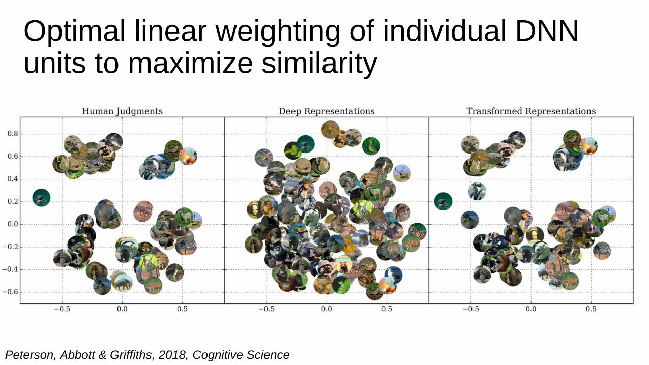
Optimal linear weighting of individual DNN units to maximize similarity

Peterson, Abbott & Griffiths, 2018, Cognitive Science

Regression-based encoding methods

Encoding: X Y

Simple multiple linear regressionp

vo

xels

n conditions

q u

nit

s

n conditions

DNN layer activationsBrain (e.g. fMRI betas)

Simple multiple linear regression

p voxels

n c

on

dit

ion

s

Brain (e.g. fMRI betas)

q units

n c

on

dit

ion

s

DNN layer activations

Simple multiple linear regression

voxel i

n c

on

dit

ion

s

y = X β ε+

q units

n c

on

dit

ion

s

•

Brain (e.g. fMRI betas) DNN layer activations

Repeat for each voxel (i.e. univariate method)

Brain (e.g. fMRI betas) DNN layer activations

Simple multiple linear regression

voxel i

n c

on

dit

ion

s

y = X β ε+

q units

n c

on

dit

ion

s

•

Problem: Often more variables (q units) than measurements (n conditions) no unique solution, unstable parameter estimates and overfitting

One solution: Regularization, i.e. adding constraints on the range of values β can take (e.g. Ridge regression, LASSO regression)

Another solution: Dimensionality reduction, i.e. projecting data to a subspace (e.g. Principal Component regression, Partial Least Squares)

Regularization in multiple linear regression

Formula for regression:

Error minimized for OLS regression:

Error minimized for ridge regression:

Error minimized for LASSO regression:

(y − 𝑋ß)²

𝑦 = 𝑋ß + ε

(y − 𝑋ß)² + λ𝑟 ß ²

Constrains range

of beta

(y − 𝑋ß)² + λ𝑙 ß

Requires optimization of regularization parameter 𝛌 (e.g. using cross-validation)

Advanced regularization: explicit assumptions on covariance matrix structure

Regularization in multiple linear regression

Formula for regression:

Error minimized for OLS regression:

Error minimized for ridge regression:

Error minimized for LASSO regression:

(y − 𝑋ß)²

𝑦 = 𝑋ß + ε

(y − 𝑋ß)² + λ𝑟 ß ²

Constrains range

of beta

(y − 𝑋ß)² + λ𝑙 ß

Requires optimization of regularization parameter 𝛌 (e.g. using cross-validation)

Advanced regularization: explicit assumptions on covariance matrix structure

quality of fit can be estimated using cross-validation(e.g. split-half or 90%-10% split)

Presence of many variables leads to potential for overfitting

Results: Regression-based encoding methods

Monkey V4 and IT

• 5760 images of 64

objects (8 categories)

• custom DNN “HMO”

Human visual cortex

Yamins et al., 2014, PNAS Güçlü & van Gerven, 2015, J Neurosci

Voxelwise prediction Most predictive layer

• 1750 images

• DNN: AlexNet variant

Building networks to model the brain

Recurrent models better capture core object recognition in ventral visual cortex

in both monkey recordings… … and humans (MEG sources)

Kietzmann, et al., 2018, bioRxivKar et al., 2019, Nat Neurosci

Practical considerations

Matlab users: Using MatConvNet

• Downloading pretrained models:

http://www.vlfeat.org/matconvnet/pretrained/

• Quick guide to getting started:

http://www.vlfeat.org/matconvnet/quick/

• Function for getting layer activations:

http://martin-hebart.de/code/get_dnnres.m

Python users: Using Keras

• Keras is very easy, but classic TensorFlow or PyTorch also work

• Running images through pretrained models:

https://engmrk.com/kerasapplication-pre-trained-model/

• Getting layer activations (still requires preprocessing images):

https://github.com/philipperemy/keract

If goal is maximizing brain prediction:

• Pick network with most predictive layer(s)

• Brain score?

If goal is using plausible model:

• Very common / better understood architectures: AlexNet and VGG-16

• Other architectures (e.g. ResNet, DenseNet) less common

What architecture should we pick?

Schrimpf, Kubilius et al., 2018, bioRxiv

If goal is to maximize brain prediction

Try all layers

If goal is using entire DNN as model of brain

Try all or some layers

If goal is using plausible model where layer progression mirrors progression in brain: some layers

Pick plausible layers

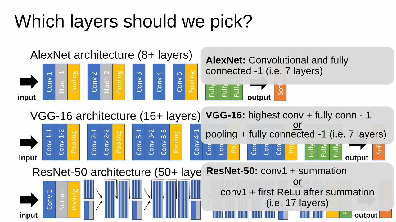
Which layers should we pick?

Which layers should we pick?

AlexNet architecture (8+ layers)C

on

v 1

No

rm 1

Poo

ling

Co

nv

2

No

rm 2

Poo

ling

Co

nv

3

Co

nv

4

Co

nv

5

Poo

ling

Fully

co

nn

Fully

co

nn

Fully

co

nn

Soft

max

input output

Co

nv

1-1

Co

nv

1-2

Poo

ling

Co

nv

2-1

Co

nv

2-2

Poo

ling

Co

nv

3-1

Co

nv

3-2

Co

nv

3-3

Poo

ling

Co

nv

4-1

Co

nv

4-2

Co

nv

4-3

Poo

ling

Co

nv

5-1

Co

nv

5-2

Co

nv

5-3

Poo

ling

Fully

co

nn

Fully

co

nn

Fully

co

nn

Soft

max

input output

VGG-16 architecture (16+ layers)

ResNet-50 architecture (50+ layers)

Co

nv

1

input

No

rm 1

Poo

ling

Poo

ling

Fully

co

nn

Soft

max

output

Which layers should we pick?

AlexNet architecture (8+ layers)C

on

v 1

No

rm 1

Poo

ling

Co

nv

2

No

rm 2

Poo

ling

Co

nv

3

Co

nv

4

Co

nv

5

Poo

ling

Fully

co

nn

Fully

co

nn

Fully

co

nn

Soft

max

input output

Co

nv

1-1

Co

nv

1-2

Poo

ling

Co

nv

2-1

Co

nv

2-2

Poo

ling

Co

nv

3-1

Co

nv

3-2

Co

nv

3-3

Poo

ling

Co

nv

4-1

Co

nv

4-2

Co

nv

4-3

Poo

ling

Co

nv

5-1

Co

nv

5-2

Co

nv

5-3

Poo

ling

Fully

co

nn

Fully

co

nn

Fully

co

nn

Soft

max

input output

VGG-16 architecture (16+ layers)

ResNet-50 architecture (50+ layers)

Co

nv

1

input

No

rm 1

Poo

ling

Poo

ling

Fully

co

nn

Soft

max

output

Should we include highest fully-connected layer (1000-D)?

Pro:• Output of computation from neural network at highest levelCon:• Emphasis of categories represented as classes, may introduce

positive or negative bias in results

My suggestion: Exclude layer

Which layers should we pick?

AlexNet architecture (8+ layers)C

on

v 1

No

rm 1

Poo

ling

Co

nv

2

No

rm 2

Poo

ling

Co

nv

3

Co

nv

4

Co

nv

5

Poo

ling

Fully

co

nn

Fully

co

nn

Fully

co

nn

Soft

max

input output

Co

nv

1-1

Co

nv

1-2

Poo

ling

Co

nv

2-1

Co

nv

2-2

Poo

ling

Co

nv

3-1

Co

nv

3-2

Co

nv

3-3

Poo

ling

Co

nv

4-1

Co

nv

4-2

Co

nv

4-3

Poo

ling

Co

nv

5-1

Co

nv

5-2

Co

nv

5-3

Poo

ling

Fully

co

nn

Fully

co

nn

Fully

co

nn

Soft

max

input output

VGG-16 architecture (16+ layers)

ResNet-50 architecture (50+ layers)

Co

nv

1

input

No

rm 1

Poo

ling

Poo

ling

Fully

co

nn

Soft

max

output

AlexNet: Convolutional and fully connected -1 (i.e. 7 layers)

VGG-16: highest conv + fully conn - 1or

pooling + fully connected -1 (i.e. 7 layers)

ResNet-50: conv1 + summationor

conv1 + first ReLu after summation(i.e. 17 layers)

Common preprocessing of images

My advice:

• Run studies on participants / animals using square images

• Resize and crop images to correct size before running toolbox function provides maximal control

• Make sure image normalization is implemented and correct

Original image 2. Crop to square

and keep 7/8th

1. Resize 3. Normalize (e.g. z-

score or subtract mean

image during training)

Reduction of model size

• Useful when predicting brain data from layers with many units• Makes more complex models possible at all

• increases computational speed

• can reduce overfitting

• Examples:• AlexNet Layer 1: 55×55×96 = 290,400 units

• VGG-16 / ResNet Layer 1: 112×112×64 = 802,816 units

Common approach: PCA compression

PCA compression of DNN layer

Step 1: Get ImageNet validation set of

50,000 images (possibly include test set of

150,000 images)

Step 2: Push images through network in

batches, extract layer activation, flatten and

store on hard drive

Step 3: Run incremental PCA or random projection (e.g. in scikit-learn), set number of PCs to a reasonable number (e.g. 1000)

PC1PC2

Step 4: Save PCA model, push new images through network, extract layer activation, flatten and apply transformation from PCA

Take-home messages

Comparing brains and DNNs is easy, but what to do with it is harder

Common methods to map DNNs and brains are regression-based and similarity-based encoding methods

DNNs often treated only loosely as brain model (e.g. taking all layers to predict activity in V1)

Even older models (e.g. AlexNet) perform well and are still common