Comparing Business Processes to Determine theFeasibility of Configurable Models: A Case Study

J.J.C.L. Vogelaar, H.M.W. Verbeek, B. Luka, and W.M.P van der Aalst

Technische Universiteit EindhovenDepartment of Mathematics and Computer Science

P.O. Box 513, 5600 MB Eindhoven, The Netherlands{h.m.w.verbeek,w.m.p.v.d.aalst}@tue.nl

Abstract. Organizations are looking for ways to collaborate in the area of pro-cess management. Common practice until now is the (partial) standardization ofprocesses. This has the main disadvantage that most organizations are forced toadapt their processes to adhere to the standard. In this paper we analyze andcompare the actual processes of ten Dutch municipalities. Configurable processmodels provide a potential solution for the limitations of classical standardiza-tion processes as they contain all the behavior of individual models, while onlyneeding one model. The question rises where the limits are though. It is ob-vious that one configurable model containing all models that exist is undesir-able. But are company-wide configurable models feasible? And how about cross-organizational configurable models, should all partners be considered or just cer-tain ones? In this paper we apply a similarity metric on individual models todetermine means of answering questions in this area. This way we propose anew means of determining beforehand whether configurable models are feasible.Using the selected metric we can identify more desirable partners and processesbefore computing configurable process models.

Key words: process configuration, YAWL, CoSeLoG, model merging

1 Introduction

The results in this paper are based on 80 process models retrieved for 8 different busi-ness processes from 10 Dutch municipalities. This was done within the context of theCoSeLoG project [1, 6]. This project aims to create a system for handling various typesof permits, taxes, certificates, and licenses. Although municipalities are similar in thatthey have to provide the same set of business processes (services) to their citizens, theirprocess models are typically different. Within the constraints of national laws and reg-ulations, municipalities can differentiate because of differences in size, demographics,problems, and policies. Supported by the system to be developed within CoSeLoG, in-dividual municipalities can make use of the process support services simultaneously,even though their process models differ. To realize this, configurable process modelsare used.

Configurable process models form a relatively young research topic [8, 12, 13, 3].A configurable process model can be seen as a union of several process models intoone. While combining different process models, duplication of elements is avoided by

2 J.J.C.L. Vogelaar, H.M.W. Verbeek, B. Luka, and W.M.P van der Aalst

matching and merging them together. The elements that occur in only a selection of theindividual process models are made configurable. These elements are then able to beset or configured. In effect, such an element can be chosen to be included or excluded.When for all configurable elements such a setting is made, the resulting process model iscalled a configuration. This configuration could then correspond to one of the individualprocess models for example.

Configurable process models offer several benefits. One of the benefits is that thereis only one process model that needs to be maintained, instead of the several individualones. This is especially helpful in case a law changes or is introduced, and thus allmunicipalities have to change their business processes, and hence their process models.In the case of a configurable process model this would only incur a single change.When we lift this idea up to the level of services (like in the CoSeLoG project [1, 6]),we also only need to maintain one information system, which can be used by multiplemunicipalities.

Configurable process models are not always a good solution however. In some casesthey will yield better results than in others. Two process models that are quite similarare likely to be better suited for inclusion in a configurable process model than twocompletely different and independent process models. For this reason, this paper strivesto provide answers to the following three questions:

1. Which business process is the best starting point for developing a configurable pro-cess model? That is, given a municipality and a set of process models for everymunicipality and every business process, for which business process is the config-urable process model (containing all process models for that business process) theless complex?

2. Which other municipality is the best candidate to develop configurable modelswith? That is, given a municipality and a set of process models for every municipal-ity and every business process, for which other municipality are the configurableprocess models (containing the process models for both municipalities) the lesscomplex?

3. Which clusters of municipalities would best work together, using a common con-figurable model? That is, given a business process and a set of process models forevery municipality and every business process, for which clustering of municipal-ities are the configurable process models (containing all process models for themunicipalities in a cluster) the less complex?

The remainder of this paper is structured as follows. Section 2 discusses the tech-niques used in this paper to answer the proposed questions. Section 3 then introduces the80 process models and background information about these process models. Section 4makes various comparisons to produce answers to the proposed questions. Finally, Sec-tion 5 concludes the paper.

Comparing Business Processes to Determine the Feasibility of Configurable Models 3

2 Preliminaries

2.1 YAWL

This paper presents several business processes modeled in YAWL (Yet Another Work-flow Language) [9]. YAWL allows for the basic components that are present in theprocess models obtained from the municipalities. It is a workflow language developedby the YAWL Foundation and based on the Workflow Patterns [4]. Figure 1 shows anannotated example YAWL model.

Fig. 1: An annotated example YAWL model

A YAWL model basically consists of conditions (circles), tasks (rectangles) andconnectors (arrows). The connectors indicate the flow of control in a YAWL model,where each undecorated task can only have one incoming and one outgoing connector.The YAWL model in Figure 1 should be read from left tot right. The element furthest tothe left is the start condition, which corresponds to the start of the process. The end ofthe process is located all the way to the right. A YAWL model can only have one startand one end condition.

A task can be a normal task (like “Fill in e-form”), or act as a branching node (like“Decide admissible”) in the process model. If the latter is the case, then the task has adecorator to indicate whether it is an AND-join (or -split), an XOR-join (or -split), or anOR-join (or -split). XOR-splits (like “Decide admissible”) introduce choice brancheswhere one of the offered choices can be followed, whereas XOR-joins (like “XORjoin”) merge alternative flows. AND-splits (like “Determine fees”) introduce parallelbranches, whereas AND-joins (like “AND join”) merge parallel branches. OR-splits(not present) introduce a (non-empty) subset of parallel branches, whereas OR-joins(not present) merge a subset of those branches by waiting until the remaining branchesare dead. Conditions (like “Waiting for payment”) can have multiple incoming or out-going connectors. This can be seen as an XOR-split/join, with the subtle differencethat this is an implicit choice [4]. It is also possible to give a task some extra meaningwhich is indicated by its decorations. A clock (like “No payment”) indicates that it is atimed task, which executes after some timer expires. A small triangle (like “XOR join”)indicates that it is an automatic task, which are mostly needed for routing purposes.

4 J.J.C.L. Vogelaar, H.M.W. Verbeek, B. Luka, and W.M.P van der Aalst

2.2 EPC models

Although the process models are presented as YAWL models, the metrics used in thispaper are typically defined on EPC (Event-driven Process Chain) models [10, 11, 16].For this reason, we also introduce EPC models.

An EPC model typically consists of functions (rectangles), events (hexagons), con-nectors (circles), and edges (arrows). Roughly spoken, EPC functions correspond toYAWL tasks, EPC events correspond to YAWL conditions, EPC connectors correspondto YAWL task decorations, and EPC edges correspond to YAWL connectors. In an EPCmodel, only connectors are allowed to have multiple input edges and/or multiple outputedges.

The conversion from a YAWL model to an EPC model is straightforward:

– A YAWL task is converted into an EPC fragment containing of a join connector, anevent, a function, a split connector, and a series of three connecting edges, where theYAWL task decorators determine the type of the EPC connectors.

– A regular YAWL condition is converted into an XOR-join connector, an XOR-splitconnector, and a connecting edge.

– The YAWL input condition is converted into an event, a (dummy) function, an XOR-split connector, and a series of two connecting edge, whereas the YAWL output con-dition is converted into an XOR-join connector, an event, and a connecting edge.

– A YAWL connector is converted into an edge.

Superfluous connectors and a possible dummy function at the start of the EPC modelwill be removed in a post-processing step. Figure 2 shows the annotated example YAWLmodel of Figure 1 converted into an EPC model.

2.3 Creating configurable models

For creating a configurable model from two different process models we use the ap-proach as described in [8]. This approach has been implemented in the “EPC merge”plug-in of the “ProM 5.2” toolkit [18, 17]. However, given the fact that we had a specificset of process models to work with, we tailored this plug-in to our needs.

When running the “EPC merge” plug-in on two EPC models, the user needs tospecify which functions of one EPC model match which functions of the second, andthe same for events. To help the user with this task, the plug-in offers a default matchwhich is based on the String-edit distance (SED) metric on the names of the functions(events): The function (event) with the smallest SED value will be selected by defaultas a match. However, in our set of YAWL models tasks were considered to be identicalif their names were identical. On the EPC level, this corresponds to the requirementthat function and event names should be identical modulo some trailing underscore andnumber, which are added by the YAWL editor automatically. As a result, two functionsnamed “Fill in e-form 11” and “Fill in e-form 36” should be considered to be identi-cal. Furthermore, we sometimes needed to duplicate a YAWL task, while the YAWLeditor does not allow for duplicate names. In such a case, we simply added a num-ber to the end of the task name. For example, “Fill in e-form” would become “Fill ine-form1”. The matching algorithm takes these trailing number also into account, and

Comparing Business Processes to Determine the Feasibility of Configurable Models 5

Fig. 2: The annotated example YAWL model converted into an EPC

6 J.J.C.L. Vogelaar, H.M.W. Verbeek, B. Luka, and W.M.P van der Aalst

is able to match “Fill in e-form 11” with “Fill in e-form1 36”. As some minor typoscould be present in the names of the YAWL models, we decided to allow for a singletypo. As a result, the SED value between two matching names was allowed to be atmost one. Hence, “Fill in eform 11” would be matched with “Fill in e-form1 36”. Fi-nally, there was no reason to match different joins and/or splits in the models, as therewas no guarantee that a correct match could be found for these dummy functions anddummy events. As a result, we decided to remove any match from a function or eventsthat was named like “AND join 11”, “status change to XOR split1 36” etc.

2.4 Graph-edit distance similarity

This paper strives to give an answer to a couple of questions about models. To answerthese questions, the models need to be compared to each other. There has been extensiveresearch into the comparison of models on different levels and in different modelinglanguages [7, 19, 22]. In this paper we limit ourselves to using the Graph-Edit Distance(GED) similarity metric and the Structural process similarity (SPS) metric, which wereintroduced in [7].

The GED metric is a structural metric based on the minimal number of graph-editoperations needed to transform one graph into an other, taking node deletion, nodeinsertion, node substitution, edge deletion, edge insertion into account. Let M : (N1 9N2) be the partial injective mapping that induces the GED between two process modelsand let sn be the set of all inserted and deleted nodes, se be the set of all inserted anddeleted edges and let Sim(n,m) be a function that assigns a similarity score to a pairof nodes. As shown in [7], a similarity metric is gained from the graph-edit distancemetric by calculating:

simGED(G1, G2) = 1− snv + sev + sbv

3,

where:

snv =|sn|

|N1|+ |N2|;

sev =|se|

|E1| + |E2|;

sbv =2 ·Σ(n,m)∈M1− Sim(n,m)

|N1|+ |N2| − |sn|.

(1)

The “graph similarity” plug-in of ProM 5.2 was used (with default settings) to com-pare the different YAWL models to each other on the EPC level, that is, we first convertboth YAWL models to EPC models as described earlier, and compare the resulting EPCmodels instead.

2.5 Structural process similarity

The SPS metric also considers the EPC to be plain labeled graphs, but uses a combina-tion of:

Comparing Business Processes to Determine the Feasibility of Configurable Models 7

Syntactic similarity, which considers only the syntax of the labels,Semantic similarity, which abstracts from the syntax and looks at the semantics of the

words within the labels, andContextual similarity, which considers not only the labels of the elements themselves,

but also the context (surrounding nodes) in which these elements occur.

These metrics determine the similarity score between pairs of elements in the two mod-els. The overall metric has been implemented in the Process Similarity tool, which ispart of the Synergia toolset. For any two EPCs that are provided as input, the ProcessSimilarity tool calculates their SPS similarity, which is a decimal value between 0 and1, where 1 means that the processes are identical.

2.6 Control-flow complexity (CFC)

Aside from the comparison between models, the paper also strives to give complexitymeasures of individual models [15]. One of the metrics used is the control-flow com-plexity (CFC) as introduced in [5]:

CFC(GEPC) =∑

n∈NS

CFC(n)

where GEPC = (NF ∪NE ∪NC , E) is the corresponding EPC model with functionsNF , events NE , connectors NC , and edges E, and NS is the set of split nodes (NS ⊆NC). For a split node n ∈ NS with fan out k (number of output arcs):

CFC(n) =

1 if n is an AND-split;k if n is an XOR-split;2k if n is an OR-split.

The “EPC complexity analysis” plug-in of ProM 5.2 was used to determine theCFC metric. Again, we first convert the YAWL model at hand to an EPC model, anddetermine the CFC of the resulting EPC model instead. The CFC metric of the YAWLmodel as shown by Figure 1 yields 2 + 2 + 1 = 5, as in the resulting EPC model (seeFigure 2) both XOR-split connectors have CFC value 2 and the AND-split connectorhas CFC value 1.

2.7 Density

Another complexity metric used in this paper, is the density metric as discussed in [15].In general, for a graph G = (N,E) with nodes N and edges E, this metric correspondsto the number of actual arcs divided by the maximal number of possible arcs, which canbe computed as

Density(G) =|E|

|N | · (|N | − 1)

However, for an EPC model GEPC = (NF ∪NE ∪NC , E) with functions NF , eventsNE , connectors NC , and edges E we know that functions and events do not allow for

8 J.J.C.L. Vogelaar, H.M.W. Verbeek, B. Luka, and W.M.P van der Aalst

multiple input and/or output edges. Therefore, for computing the density metric we takeonly the connectors into account by using

Density(GEPC) =|E| − |NF | − |NE ||NC | · (|NC | − 1)

This metric is computed with the help of “EPC complexity analysis” plug-in ofProM 5.2, and in a similar way. However, the density metric as returned by this plug-indoes not correspond to the density metric as defined in [15]. Instead, it corresponds tothe density metric as defined in [14]. Luckily, from the former density metric we couldquite easily compute the latter density metric. The density metric of the YAWL modelshown by Figure 1 yields 38−14−15

6·5 = 0.3.

2.8 Cross-connectivity (CC)

A third density metric is the cross-connectivity metric (CC) as defined in [20]. Thismetric computes the maximal weights for any path between every two nodes, and di-vides this by the number of paths between every two nodes. The weight of a path equalsthe product of the weight of the nodes on this path, where:

– the weight of an XOR connector equals 1d (where d is the degree of the node, that is,

the total number of input and output arcs of the node),– the weight of an OR connector equals 1

2d+1+ 2d−2

2d−1 ·1d , and

– the weight of every other node (functions, events, AND connectors) equals 1.

In contrast to the other two complexity metrics, which are assumed to be better if lower,the CC metric is assumed to be better if higher.

This metric is computed as well by the “EPC complexity analysis” plug-in of ProM5.2. However, the computation by this plug-in for computing this metric suffers fromtwo problems: it runs out of space, and it runs out of time. The first problem was solvedby a rearrangement of the algorithm, whereas the second problem was tackled by impos-ing a weight threshold to any path under consideration: A path will only be extended ifits current weight exceeds this threshold. The CC metric of the YAWL model as shownby Figure 1 yields approx. 0.1169.

2.9 k-means clustering

k-means clustering is a standard technique to partition a data set into k clusters. First,k initial cluster centers are determined (randomly) and each data element is assigned tothe closest of these centers. The center of each cluster is recomputed (take the averageof all its data elements) and the data elements are again assigned to the closest of thesecenters. This is repeated several times to find k cluster centers with minimal distancesto elements corresponding to these centers. We will use k-means clustering to find pro-cesses and municipalities that are most similar, and we will use “Weka 3.6.5” to do thisclustering with the following parameters:

Scheme:weka.clusterers.SimpleKMeans -N 3 -A ”weka.core.EuclideanDistance-R first-last” -I 500 -S 10

Comparing Business Processes to Determine the Feasibility of Configurable Models 9

that is, find 3 clusters, use Euclidian distance, do 500 iterations, and use 10 as the initialseed.

3 YAWL models

We collected 80 YAWL models in total. These YAWL models were retrieved fromthe ten municipalities, which are partners in the CoSeLoG project: Bergeijk, Bladel,Coevorden, Eersel, Emmen, Gemert-Bakel, Hellendoorn, Oirschot, Reusel-de Mierdenand Zwolle. In the remainder of this paper we will refer to these municipalities as MunA

to MunJ (these are randomly ordered).Five of the mentioned municipalities started working together in 2010. They share

a service center, which provides most of the IT-support the municipalities need. Theyalso share a social services provider. The remaining five municipalities also work to-gether in the IT-area, but to a lesser extent: They make use of a commonly developedsoftware system (hosted individually). This system is meant to handle the front-end ofall participating municipalities in a similar way, and gets expanded to provide compre-hensive workflow support. Needless to say, both these groups of municipalities couldgreatly benefit from the use of configurable models as they have to deliver the same setof services.

For every municipality, we retrieved the YAWL models for the same eight businessprocesses, which are run by any Dutch municipality. Hence, our process model collec-tion is composed of eight sub-collections consisting of ten YAWL models each. TheYAWL models were retrieved through interviews by us and validated by the municipal-ities afterwards.

The eight business processes covered are:

1. The processing of an application for a receipt from the people registration (3 vari-ants):a) When a customer applies through the internet: GBA1.b) When a customer applies in person at the town hall: GBA2.c) When a customer applies through a written letter: GBA3.

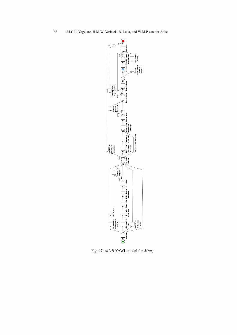
2. The method of dealing with the report of a problem in a public area of the munici-pality: MOR.

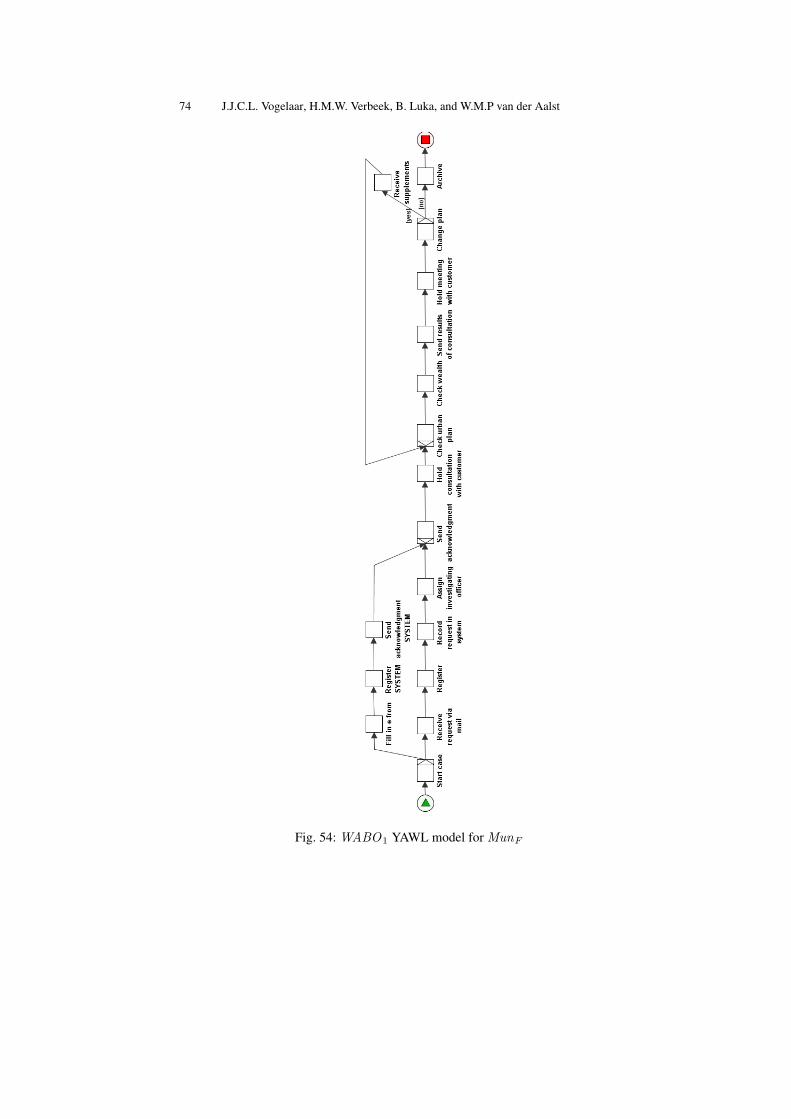
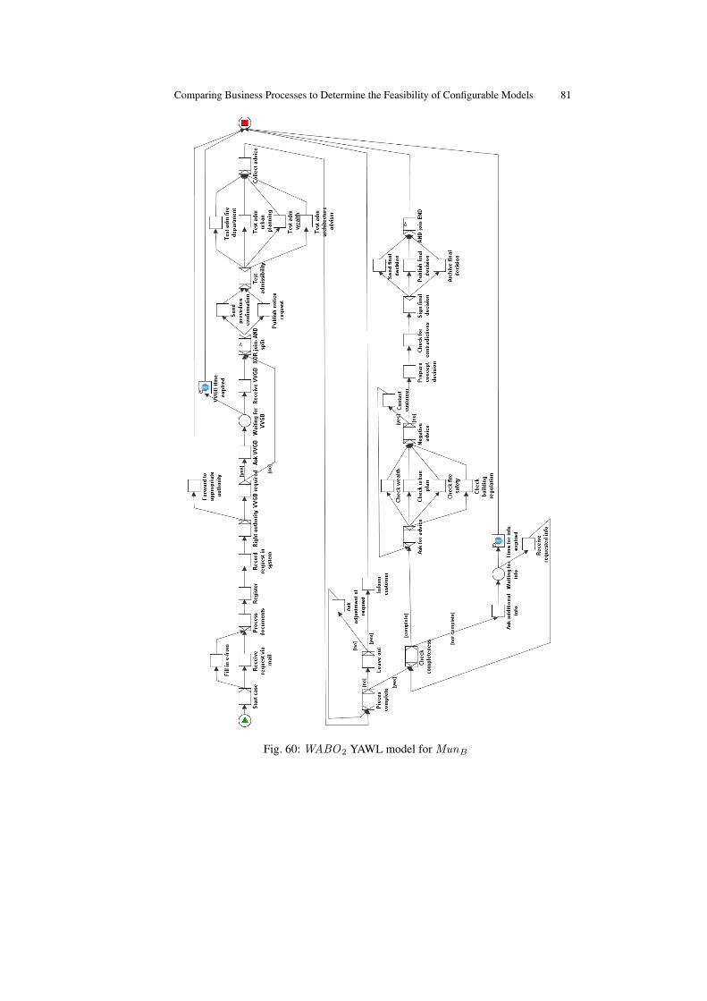
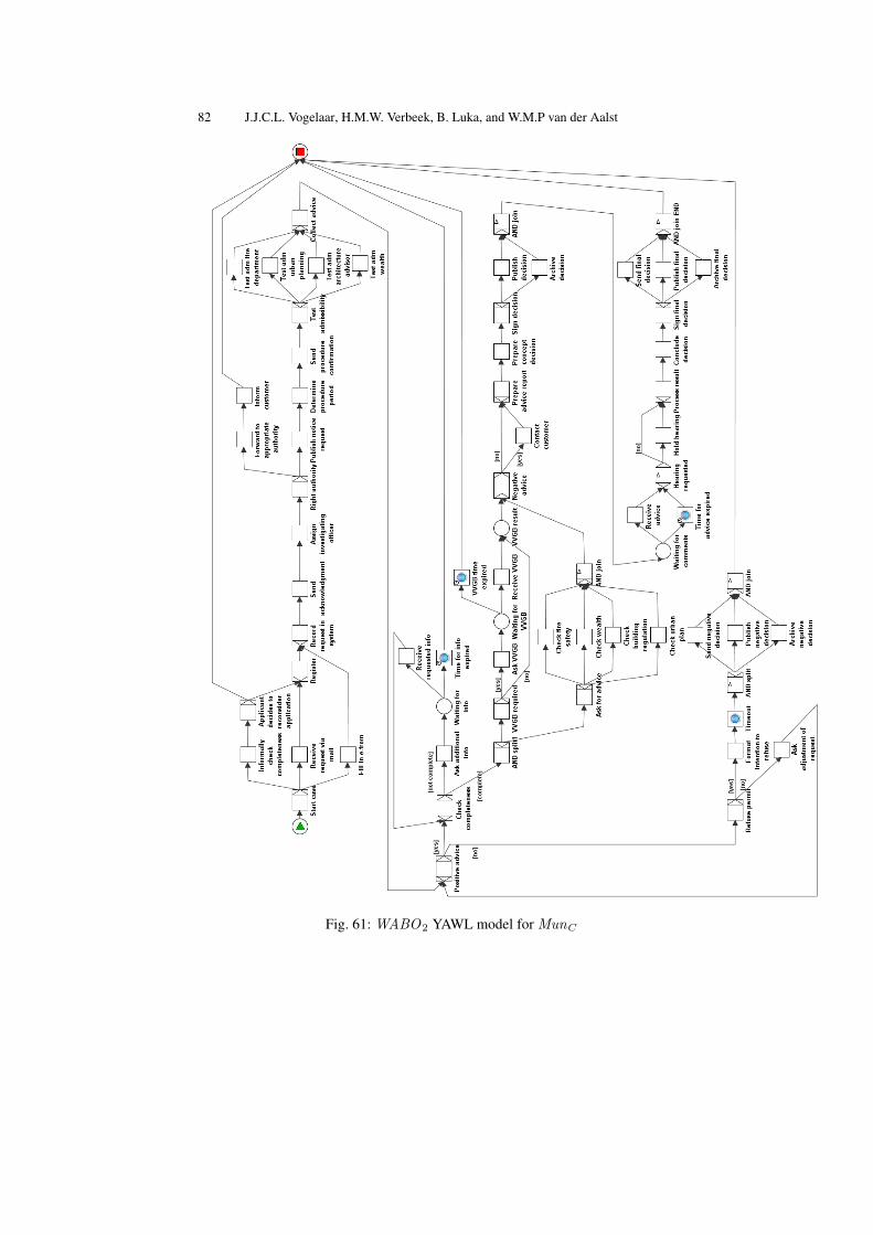
3. The processing of an application for a building permit (2 parts):a) The preceding process to prepare for the formal procedure: WABO1.b) The formal procedure: WABO2.

4. The processing of an application for social services: WMO .5. The handling of objections raised against the taxation of a house: WOZ .

To give an indication of the variety and similarity between the different YAWLmodels some examples are shown. Figure 3 shows the GBA1 YAWL model of MunE ,whereas Figure 1 showed the GBA1 YAWL model of MunG. The YAWL models ofthese two municipalities are quite similar. Nevertheless, there are some differences. Re-call that GBA1 is about the application for a certain document through the internet. Thedifference between the two municipalities is that MunE handles the payment throughthe internet (so before working on the document), while MunG handles it manually

10 J.J.C.L. Vogelaar, H.M.W. Verbeek, B. Luka, and W.M.P van der Aalst

Fig. 3: GBA1 YAWL model for MunE

after having sent the document. However, the main steps to create the document arethe same. This explains why the general flow of both models is about the same, withexception of the payment-centered elements.

Fig. 4: GBA2 YAWL model for MunE

People can apply for this document through different means too. Figure 4 shows theGBA2 YAWL model for MunE . This model seems to contain more tasks than eitherof the GBA1 models. This makes sense, since more communication takes place duringthe application. The employee at the town hall needs to gain the necessary informationfrom the customer. In the internet case, the customer had already entered the informa-tion himself in the form, because otherwise the application could not be sent digitally.As the YAWL model still describes a way to produce the same document, it is to be ex-pected that GBA2 models are somewhat similar to GBA1 models. Indeed, the generalflow remains approximately the same, although some tasks have been inserted. Thisis especially the case in the leftmost part of the model, which is the part where in theinternet case the customer has already given all information prior to sending the digitalform. In the model shown in Figure 4 the employee asks the customer for information inthis same area. This extra interaction also means more tasks (and choices) in the YAWLmodel.

Figure 5 shows the WOZ YAWL model for MunE , which is clearly different fromthe three GBA models. The WOZ model shown in Figure 5 is more time-consuming.Customers need to be heard and their objections need to be assessed thoroughly. Next,the grounds for the objections need to be investigated, sometimes even leading to ahouse visit. After all the checking and decision making has taken place, the decisionneeds to be communicated to the customer, several weeks or months later. The WOZ

Comparing Business Processes to Determine the Feasibility of Configurable Models 11

Fig. 5: WOZ YAWL model for MunE

Table 1: Complexity metrics GBA1 process

MunA MunB MunC MunD MunE MunF MunG MunH MunI MunJ

CFC 6 5 4 5 7 5 5 6 5 3Density 0.350 0.400 0.667 0.350 0.300 0.350 0.300 0.350 0.350 0.417

CC 0.078 0.205 0.172 0.167 0.108 0.180 0.117 0.078 0.180 0.184

models are quite a bit different from the GBA models, where information basicallyneeds to be retrieved and documented.

The remainder of this paper presents a case study of the 80 YAWL models (whichcan found in Appendix A), and compares them within their own sub-collections. Thisway, we show that the YAWL models for the municipalities are indeed different, but notso different that it justifies the separate implementation and maintenance of ten separatesoftware systems.

4 Comparison

This section compares all YAWL models from each of the sub-collections. As certainmodels are more similar than others, we want to give an indication on which processesare very similar, and which are more different. This similarity we will use as an indi-cation of which models have more or less complexity when merged into a configurablemodel. The higher the similarity between models, the lower we expect the complexityto be for the configurable models. Making a configurable model for equivalent models(similarity score 1.0) approximately results in the same model again (additional com-plexity approx. 0.0), since no new functionality needs to be added to any of the originalmodels.

First, we apply the complexity metrics as discussed earlier to all YAWL models.Second, we compare the models using the GED similarity metric as described in [7].Third and last, we answer the three questions as proposed earlier using these metrics.

4.1 Complexity

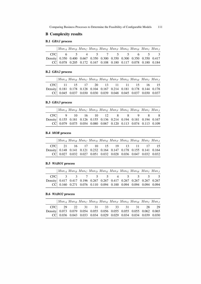
For every YAWL model, we calculated the CFC, density, and CC metric to get anindication of its complexity. The results can be found in Appendix B. As an example,

12 J.J.C.L. Vogelaar, H.M.W. Verbeek, B. Luka, and W.M.P van der Aalst

Table 2: Comparison of the business processes on the complexity metrics.

GBA1 GBA2 GBA3 MOR WABO1 WABO2 WMO WOZ

CFC 5.100 14.400 9.800 15.400 4.700 29.800 33.800 12.000Density 0.383 0.165 0.170 0.159 0.305 0.061 0.080 0.132

CC 0.147 0.038 0.088 0.035 0.119 0.034 0.024 0.064

Unified 5 15 9 17 5 30 33 13

Table 3: GED similarities GBA1 Process

MunA MunB MunC MunD MunE MunF MunG MunH MunI MunJ

MunA 1.000 0.837 0.817 0.883 0.845 0.803 0.667 1.000 0.942 0.698MunB 0.837 1.000 0.772 0.915 0.841 0.842 0.708 0.837 0.896 0.769MunC 0.817 0.772 1.000 0.807 0.799 0.798 0.665 0.817 0.798 0.664MunD 0.883 0.915 0.807 1.000 0.884 0.891 0.719 0.883 0.950 0.801MunE 0.845 0.841 0.799 0.884 1.000 0.851 0.732 0.845 0.908 0.858MunF 0.803 0.842 0.798 0.891 0.851 1.000 0.711 0.803 0.879 0.793MunG 0.667 0.708 0.665 0.719 0.732 0.711 1.000 0.667 0.717 0.723MunH 1.000 0.837 0.817 0.883 0.845 0.803 0.667 1.000 0.942 0.698MunI 0.942 0.896 0.798 0.950 0.908 0.879 0.717 0.942 1.000 0.793MunJ 0.698 0.769 0.664 0.801 0.858 0.793 0.723 0.698 0.793 1.000

Table 1 shows the complexity metrics for all GBA1 models. Figure 6 shows the relationbetween the CFC metric and the other two complexity metrics. Clearly, these relationsare quite strong: The higher the CFC metric, the lower the other two metrics. Althoughthis is to be expected for the CC metric, this is quite unexpected for the density metric.Like the CFC metric, the density metric was assumed to go up when complexity goesup, hence the trend should be that the density metric should go up when the CFC metricgoes up. Obviously, this is not the case. As a result, for the remainder of this paper wewill assume that the density metric goes down when complexity goes up.

Based on the strong relations as suggested in Figure 6 (CC(G) = 0.4611 ·CFC(G)−0.851 and density(G) = 1.1042 · CFC(G)−0.791) we can now transformthe other two complexity metrics to the scale of the CFC metric. As a result, we cantake the rounded average over the resulting three metrics and get a unified complexitymetric. Table 2 shows the average complexity metrics for all business processes. As thistable shows, the processes WABO2 and WMO are the most complex, and GBA1 andWABO1 the least complex.

4.2 Similarity

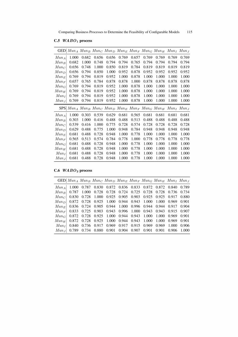
For every pair of YAWL models from the same sub-collection, we calculated the GEDand SPS metric to get an indication of their similarity. The results can be found inAppendix C. As an example, Table 3 shows the GED similarity metrics for the GBA1

YAWL models. In the table, the minimum is 0.664 and the maximum element (ex-cluding the main diagonal) is 1.000. Figure 7 shows the relation between the GED

Comparing Business Processes to Determine the Feasibility of Configurable Models 13

Fig. 6: Comparison of the CFC metric with the CC and Density metrics.

14 J.J.C.L. Vogelaar, H.M.W. Verbeek, B. Luka, and W.M.P van der Aalst

Fig. 7: Comparison of the GED metric with the SPS metric.

Comparing Business Processes to Determine the Feasibility of Configurable Models 15

Table 4: Average similarity values

GBA1 GBA2 GBA3 MOR WABO1 WABO2 WMO WOZ

GED 0.829 0.916 0.828 0.797 0.871 0.891 0.830 0.820SPS 0.646 0.759 0.632 0.556 0.774 0.725 0.546 0.615

Unified 0.632 0.778 0.624 0.554 0.739 0.735 0.583 0.607

and the SPS metric. Although the relation between these metrics (SPS(G1, G2) =2.0509 · GED(G1, G2) − 1.082) is a bit less strong as the relation between the com-plexity metrics, we consider this relation to be strong enough to unify both metrics intoa single, unified, metric. This unified similarity metric uses the scale of the SPS metric,as the range of this scale is wider than the scale of the GED metric. Table 4 shows theaverages over the values for the different similarity metrics for each of the processes.From this table, we conclude that the GBA2 models are most similar to each other,while the MOR models are least similar.

Recall that a configurable process model “contains” all individual process models.Whenever one wants to use the configurable model as an executable model, it needsto be configured by selecting which parts should be left out. The more divergent theindividuals are, the more complex the resulting configurable process model needs tobe to accommodate all the individuals. So, the more similar models are, the easier toconstruct and maintain the configurable model will most likely be.

As shown in Table 3, the similarity value for the GBA1 models for MunA andMunH equals 1.0. Merging these models into a configurable model, yields an equiva-lent model, which we find not so interesting. Taking a look at another high similarityvalue in the table, we construct the configurable GBA1 model for MunD and MunI . Thecomplexity metrics for the configurable model yield 7 (CFC), 0.238 (density), 0.091(CC), and 7 (unified). Similarly we construct a configurable model for the two least sim-ilar models: MunG and MunF . The resulting complexity values are 34 (CFC), 0.108(density), 0.026 (CC), and 28 (unified). These results are in line with our expectations,as the former metrics are all better than the latter.

To confirm these relation between similarity on the one hand and complexity on theother, we have selected 100 pairs of models (each pair from the same sub-collection),have merged every pair, and have computed the complexity metrics of the resultingmodel. Figure 8 shows the results: When similarity goes down, complexity tends to goup.

Based on the illustrated correlations, we assume that the unified similarity metricgives a good indication for the unified complexity of the resulting configurable model.Therefore, we use this metric to answer the three questions stated in the introduction.

4.3 Question 1: Which business process is the best starting point for developing aconfigurable process model?

To answer this question we select a specific business process P and compute the averagesimilarity between the YAWL model of process P in a selected municipality and all

16 J.J.C.L. Vogelaar, H.M.W. Verbeek, B. Luka, and W.M.P van der Aalst

Fig. 8: Unified similarity vs. unified complexity for 100 pairs of models.

Comparing Business Processes to Determine the Feasibility of Configurable Models 17

Table 5: Average similarity values per model

MunA MunB MunC MunD MunE MunF MunG MunH MunI MunJ

GBA1 0.631 0.612 0.560 0.703 0.645 0.641 0.354 0.631 0.715 0.442GBA2 0.766 0.821 0.667 0.602 0.807 0.771 0.751 0.821 0.725 0.821GBA3 0.530 0.513 0.486 0.607 0.550 0.587 0.678 0.551 0.678 0.664MOR 0.496 0.548 0.501 0.482 0.585 0.488 0.573 0.468 0.430 0.491

WABO1 0.501 0.483 0.602 0.776 0.818 0.662 0.818 0.818 0.818 0.818WABO2 0.646 0.419 0.730 0.800 0.746 0.741 0.800 0.800 0.750 0.644WMO 0.621 0.539 0.543 0.426 0.491 0.503 0.496 0.625 0.615 0.522WOZ 0.507 0.448 0.447 0.601 0.562 0.616 0.600 0.651 0.657 0.561

Table 6: Comparing WABO2 and WMO for MunD

WABO2 WMO

MunA 92 105MunB 72 112MunC 71 84MunE 51 95MunF 55 78MunG 32 85MunH 32 102MunI 34 102MunJ 64 82

Average 56 94

models of P in other municipalities. Take for example MunD. For the GBA1 process,the average value for MunD (that is, average distance to other municipalities) is:

0.735 + 0.777 + 0.670 + 0.741 + 0.818 + 0.430 + 0.735 + 0.898 + 0.526

9= 0.703

Table 5 shows the averages for each municipality and each business process. In this tablewe can see that for MunD the WABO2 process scores highest, followed by WABO1

and GBA1. Note that for ease of reference, we have highlighted the best (bold) andworst (italics) similarity scores per municipality. So, from the viewpoint of MunD,these three are the best candidates for making a configurable model. In a similar waywe can determine such best candidates for any of the municipalities.

We now construct configurable models for the WABO2 model for MunD and eachof the other municipalities and take the average complexity metrics for these. We dothe same for the WMO model. Table 6 shows the results. Although the complexitiesof the WABO2 models (30) and the WMO models (33) are quite similar, it is clearthat merging the latter yields worse scores on all complexity metrics than merging theformer yields. Therefore, we conclude that the better similarity between the WABO2

models resulted in a less-complex configurable model, while the worse similarity be-tween the MOR models resulted in a more-complex configurable model.

18 J.J.C.L. Vogelaar, H.M.W. Verbeek, B. Luka, and W.M.P van der Aalst

Table 7: Average similarity values per municipality

MunA MunB MunC MunD MunE MunF MunG MunH MunI MunJ

MunA 0.556 0.546 0.555 0.598 0.585 0.591 0.682 0.644 0.527MunB 0.556 0.508 0.538 0.559 0.547 0.512 0.595 0.591 0.525MunC 0.546 0.508 0.580 0.617 0.552 0.575 0.604 0.569 0.552MunD 0.555 0.538 0.580 0.638 0.630 0.642 0.702 0.717 0.619MunE 0.598 0.559 0.617 0.638 0.672 0.692 0.679 0.705 0.696MunF 0.585 0.547 0.552 0.630 0.672 0.675 0.651 0.671 0.651MunG 0.591 0.512 0.575 0.642 0.692 0.675 0.656 0.687 0.672MunH 0.682 0.595 0.604 0.702 0.679 0.651 0.656 0.801 0.664MunI 0.644 0.591 0.569 0.717 0.705 0.671 0.687 0.801 0.677MunJ 0.527 0.525 0.552 0.619 0.696 0.651 0.672 0.663 0.676

Table 8: Comparing MunH and MunA for MunD

MunH MunA

GBA1 13 13GBA2 29 38GBA3 47 34MOR 41 55

WABO1 12 16WABO2 32 92WMO 102 105WOZ 26 42

Average 38 49

From Table 5 we can also conclude that the GBA2, WABO1, and WABO2 pro-cesses are, in general, good candidates to start a configurable approach with, as theyturn out best for 5, 3, and 2 municipalities.

4.4 Question 2: Which other municipality is the best candidate to developconfigurable models with?

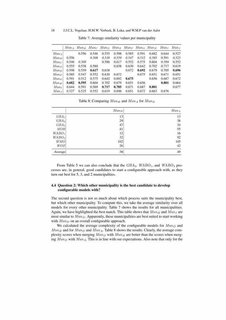
The second question is not so much about which process suits the municipality best,but which other municipality. To compute this, we take the average similarity over allmodels for every other municipality. Table 7 shows the results for all municipalities.Again, we have highlighted the best match. This table shows that MunH and MunI aremost similar to MunD. Apparently, these municipalities are best suited to start workingwith MunD on an overall configurable approach.

We calculated the average complexity of the configurable models for MunD andMunH and for MunD and MunA. Table 8 shows the results. Clearly, the average com-plexity scores when merging MunD with MunH are better than the scores when merg-ing MunD with MunA. This is in line with our expectations. Also note that only for the

Comparing Business Processes to Determine the Feasibility of Configurable Models 19

GBA3 process a configurable model with MunA might be preferred over a configurablemodel with MunH .

From Table 7 we can also conclude that MunI and MunE are preferred partners forconfigurable models, as MunI are the preferred partner for 3 of the municipalities.

4.5 Question 3: Which clusters of municipalities would best work together, usinga common configurable model?

The third question is a bit trickier to answer, but this can also be accomplished withthe computed metrics. To answer this question, we only need to consider the values inone of the comparison tables (see Appendix C). Let’s for example take Table 3. Thistable contains the similarity metrics for the GBA1 processes.e now want to see whichclusters of municipalities could best work together in using configurable models. Thereare different ways to approach this problem. One of the approaches is using the k-means clustering algorithm [2]. Applying this algorithm to the mentioned metrics, weobtain the clusters MunB +MunD +MunE +MunF +MunI , MunG +MunJ , andMunA +MunC +MunH .

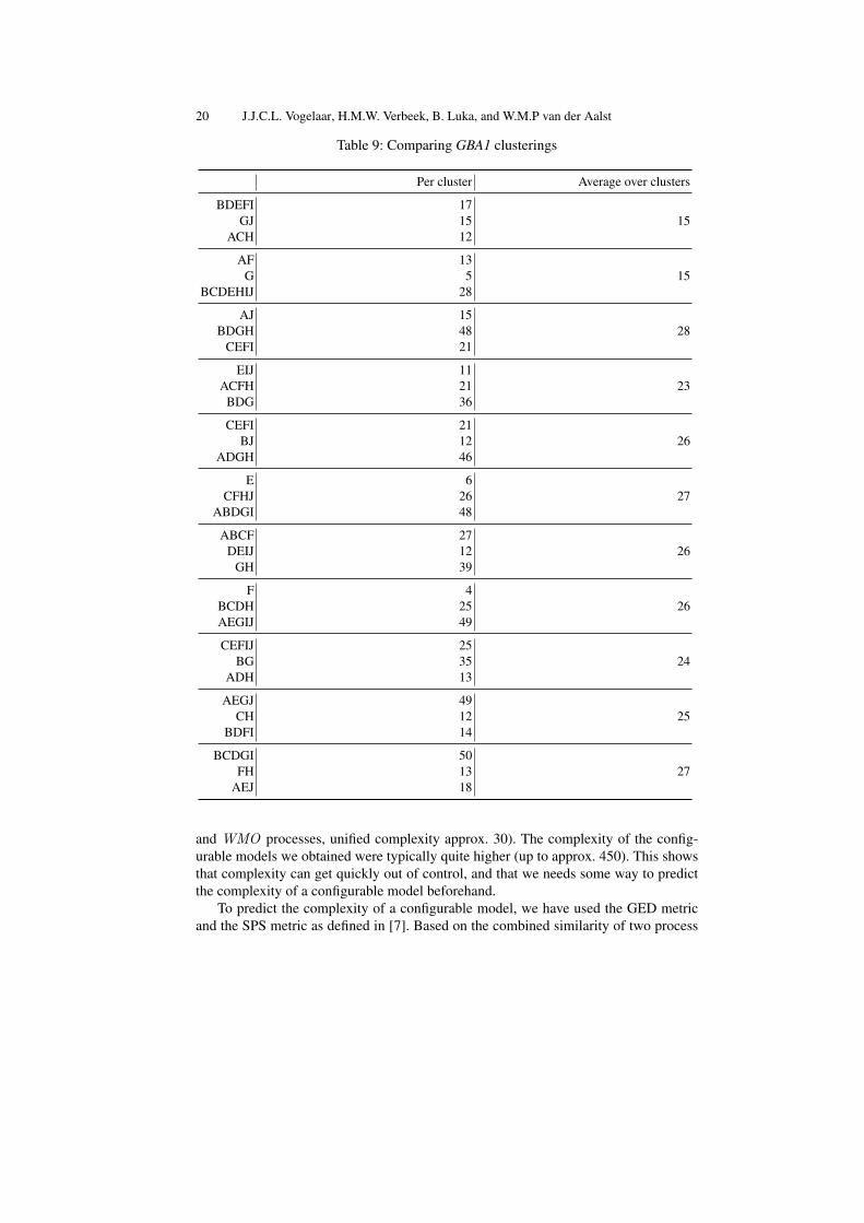
To further illustrate the correlation between the similarity and the complexity of aconfigurable model, we present Table 9, which shows the complexity metrics for theconfigurable models for the clusters obtained from the k-means clustering approach,and the metrics for the configurable models for the clusters in 10 random clusterings.Note that for sake of brevity we have simply used A for MunA etc. Observe that thecomplexity metrics for the suggested clustering are better than the metrics for any ofthe randomly selected clusters.

Table 10 shows the complexity for all processes, where cluster k is the cluster asselected by the k-means clustering technique and cluster 1 up to 10 are 10 randomlyselected clusters per process (see Appendix E for the cluster details). This table clearlyshows that the clusters as obtained by the k-means clustering technique are quite good.Only in the case of the GBA3 and WABO1 processes, we found a better clustering,and in case of the latter process the gain is only marginal.

5 Conclusion

First of all, in this paper we have shown that similarity can be used to predict the com-plexity of a configurable model. In principle, the more similar two process models are,the less complex the resulting configurable model will be.

We have used the control-flow complexity (CFC) metric from [5], the density metricfrom [15], and the cross-connectivity (CC) metric from [20] as complexity metrics. Wehave shown that these three metrics are quite related to each other. For example, whenthe CFC metric goes up, the density and CC go down. Based on this, we have been ableto unify these metrics into a single complexity metric that uses the same scale as theCFC metric.

The complexity of the 80 YAWL models used in this paper ranged from simple(GBA1 and WABO1 processes, unified complexity approx. 5) to complex (WABO2

20 J.J.C.L. Vogelaar, H.M.W. Verbeek, B. Luka, and W.M.P van der Aalst

Table 9: Comparing GBA1 clusterings

Per cluster Average over clusters

BDEFI 17GJ 15 15

ACH 12

AF 13G 5 15

BCDEHIJ 28

AJ 15BDGH 48 28

CEFI 21

EIJ 11ACFH 21 23

BDG 36

CEFI 21BJ 12 26

ADGH 46

E 6CFHJ 26 27

ABDGI 48

ABCF 27DEIJ 12 26

GH 39

F 4BCDH 25 26AEGIJ 49

CEFIJ 25BG 35 24

ADH 13

AEGJ 49CH 12 25

BDFI 14

BCDGI 50FH 13 27

AEJ 18

and WMO processes, unified complexity approx. 30). The complexity of the config-urable models we obtained were typically quite higher (up to approx. 450). This showsthat complexity can get quickly out of control, and that we needs some way to predictthe complexity of a configurable model beforehand.

To predict the complexity of a configurable model, we have used the GED metricand the SPS metric as defined in [7]. Based on the combined similarity of two process

Comparing Business Processes to Determine the Feasibility of Configurable Models 21

Table 10: Comparing clusters on CC

Cluster GBA1 GBA2 GBA3 MOR WABO1 WABO2 WMO WOZ

k 15 25 48 50 19 76 101 591 15 29 54 75 26 92 117 752 28 32 47 67 21 95 116 743 23 33 52 73 27 88 115 884 26 32 45 81 24 87 103 765 27 32 49 69 18 84 130 856 26 30 46 77 27 100 113 807 26 34 48 66 27 90 121 828 24 33 50 71 22 92 107 829 25 32 45 77 24 92 128 80

10 27 31 51 76 26 77 133 77

Average 24 31 49 71 24 88 117 78

models a prediction can be made for the complexity of the resulting configurable model.By choosing to merge only similar process models, the complexity of the resultingconfigurable model is kept at bay.

We have shown that the CFC and unified metric of the configurable model are posi-tively correlated with the similarity of its constituting process models, and that the den-sity and CC metric are negatively correlated. The behavior of the density metric cameas a surprise to us. The rationale behind this metric clearly states that a density and thelikelihood of errors are positively correlated. As such, we expected a positive correla-tion between the density and the complexity. However, throughout our set of modelswe observed the trend that less-similar models yield less-dense configurable models,whereas the other complexity metrics behave as expected. As a result, we concludedthat the density is negatively correlated with the complexity of models.

The algorithm to compute the CC metric in the “EPC complexity analysis” plug-inof ProM 5.2 was unable to cope with larger process models: It frequently ran out ofspace, and out of time. Furthermore, the density metric as computed by this plug-indoes not correspond to the density metric as defined in [15]. Instead, it corresponds tothe metric as defined in [14]. Finally, the label matching as used by the “EPC merge”plug-in of ProM 5.2 (that was used to obtain a configurable model of two processmodels) was not tailored towards our needs. As a result, we would have to changethe label match by hand, which is extremely error-prone (especially if one has to dothis many times) and would require us to remember the match for sake of reference.For these reasons, a new, tailored, version of ProM 5.2 has been build that solves theproblem with the CC metric and provides us with a tailored and good match. Thisversion can be downloaded from http://www.win.tue.nl/coselog/files/ProM-CoSeLoG-20110802.zip. The problem with the density metric has notbeen solved by this version, but the density metric as defined in [15] can be computedquite easily from the other metrics the “EPC complexity analysis” plug-in provides.

The merging of models A and B possibly differs from the merging of models Band A. As a result the order in which the merger is applied, can be important for the

22 J.J.C.L. Vogelaar, H.M.W. Verbeek, B. Luka, and W.M.P van der Aalst

complexity of the resulting configurable model. Therefore, we would like to look intothis issue and determine which order of merging is more suitable for a configurableprocess, and whether the GED metric could play a role in this. In parallel, we alsouse cross-organizational process mining [1, 2] to compare the actual processes of themunicipalities involved in CoSeLoG.

References

1. W.M.P. van der Aalst. Configurable Services in the Cloud: Supporting Variability WhileEnabling Cross-Organizational Process Mining. In International Conference on CooperativeInformation Systems (CoopIS 2010), volume 6426 of Lecture Notes in Computer Science,pages 8–25. Springer-Verlag, 2010.

2. W.M.P. van der Aalst. Process Mining: Discovery, Conformance and Enhancement of Busi-ness Processes. Springer-Verlag, 2011.

3. W.M.P. van der Aalst, M. Dumas, F. Gottschalk, A.H.M. ter Hofstede, M. La Rosa, andJ. Mendling. Preserving Correctness During Business Process Model Configuration. FormalAspects of Computing, 22:459–482, May 2010.

4. W.M.P. van der Aalst, A.H.M. ter Hofstede, B. Kiepuszewski, and A.P. Barros. WorkflowPatterns. Distributed and Parallel Databases, 14(1):5–51, 2003.

5. J. Cardoso. How to Measure the Control-flow Complexity of Web Processes and Workflows.2005.

6. CoSeLoG. Configurable Services for Local Governments (CoSeLoG) Project Home Page.www.win.tue.nl/coselog.

7. R. Dijkman, M. Dumas, B. F. van Dongen, R. Krik, and J. Mendling. Similarity of BusinessProcess Models: Metrics and Evaluation. Information Systems, 36(2):498–516, April 2011.

8. F. Gottschalk. Configurable Process Models. PhD thesis, Eindhoven University of Technol-ogy, The Netherlands, December 2009.

9. A. Hofstede, W.M.P. van der Aalst, M. Adams, and N. Russell. Modern Business ProcessAutomation: YAWL and its Support Environment. Springer-Verlag, 2009.

10. G. Keller, M. Nuttgens, and A.W. Scheer. Semantische Processmodellierung auf derGrundlage Ereignisgesteuerter Processketten (EPK). Veroffentlichungen des Instituts furWirtschaftsinformatik, Heft 89 (in German), University of Saarland, Saarbrucken, 1992.

11. G. Keller and T. Teufel. SAP R/3 Process Oriented Implementation. Addison-Wesley, Read-ing MA, 1998.

12. M. La Rosa. Managing Variability in Process-Aware Information Systems. PhD thesis,Queensland University of Technology, Brisbane, Australia, April 2009.

13. M. La Rosa, M. Dumas, A.H.M. ter Hofstede, and J. Mendling. Configurable Multi-perspective Business Process Models. Information Systems, 36(2):313–340, 2011.

14. J. Mendling. Testing Density as a Complexity Metric for EPCs. In German EPC Workshopon Density of Process Models, 2006.

15. J. Mendling, G. Neumann, and W.M.P. van der Aalst. Understanding the Occurrence ofErrors in Process Models Based on Metrics. In CoopIS 2007, volume 4803 of Lecture Notesin Computer Science, pages 113–130. Springer-Verlag, 2007.

16. A.W. Scheer. Business Process Engineering, Reference Models for Industrial Enterprises.Springer-Verlag, Berlin, 1994.

17. W. M. P. van der Aalst, B. F. van Dongen, C. Gnther, A. Rozinat, H. M. W. Verbeek, andA. J. M. M. Weijters. Prom: The process mining toolkit, September 2009.

Comparing Business Processes to Determine the Feasibility of Configurable Models 23

18. B. F. van Dongen, A. K. Alves de Medeiros, H. M. W. Verbeek, A. J. M. M. Weijters, andW. M. P. van der Aalst. The prom framework: A new era in process mining tool support. InG. Ciardo and P. Darondeau, editors, Application and Theory of Petri nets 2005, volume 3536of Lecture Notes in computer Science, pages 444–454, Miami, Florida, June 2005. Springer,Berlin, Germany.

19. B.F. van Dongen, R. Dijkman, and J. Mendling. Measuring Similarity Between BusinessProcess Models. In Proceedings of the 20th international conference on Advanced Informa-tion Systems Engineering, CAiSE ’08, pages 450–464. Springer-Verlag, 2008.

20. I. Vanderfeesten, H. Reijers, J. Mendling, W. van der Aalst, and J. Cardoso. On a Quest forGood Process Models: The Cross-Connectivity Metric. In Advanced Information SystemsEngineering, pages 480–494. Springer, 2008.

21. J. Vogelaar, B. Luka, and H. Verbeek. Comparing Business Processes to Determine theFeasibility of Configurable Models: A Case Study. Technical report, Eindhoven Universityof Technology, 2011.

22. M. Weidlich, A. Polyvyanyy, N. Desai, and J. Mendling. Process Compliance Measure-ment Based on Behavioural Profiles. In Proceedings of the 22nd international conferenceon Advanced information systems engineering, CAiSE’10, pages 499–514. Springer-Verlag,2010.

24 J.J.C.L. Vogelaar, H.M.W. Verbeek, B. Luka, and W.M.P van der Aalst

A YAWL models

A.1 YAWL models for the GBA1 process

Comparing Business Processes to Determine the Feasibility of Configurable Models 25

Fig. 9: GBA1 YAWL model for MunA

26 J.J.C.L. Vogelaar, H.M.W. Verbeek, B. Luka, and W.M.P van der Aalst

Fig. 10: GBA1 YAWL model for MunB

Comparing Business Processes to Determine the Feasibility of Configurable Models 27

Fig. 11: GBA1 YAWL model for MunC

28 J.J.C.L. Vogelaar, H.M.W. Verbeek, B. Luka, and W.M.P van der Aalst

Fig. 12: GBA1 YAWL model for MunD

Comparing Business Processes to Determine the Feasibility of Configurable Models 29

Fig. 13: GBA1 YAWL model for MunE

30 J.J.C.L. Vogelaar, H.M.W. Verbeek, B. Luka, and W.M.P van der Aalst

Fig. 14: GBA1 YAWL model for MunF

Comparing Business Processes to Determine the Feasibility of Configurable Models 31

Fig. 15: GBA1 YAWL model for MunG

32 J.J.C.L. Vogelaar, H.M.W. Verbeek, B. Luka, and W.M.P van der Aalst

Fig. 16: GBA1 YAWL model for MunH

Comparing Business Processes to Determine the Feasibility of Configurable Models 33

Fig. 17: GBA1 YAWL model for MunI

34 J.J.C.L. Vogelaar, H.M.W. Verbeek, B. Luka, and W.M.P van der Aalst

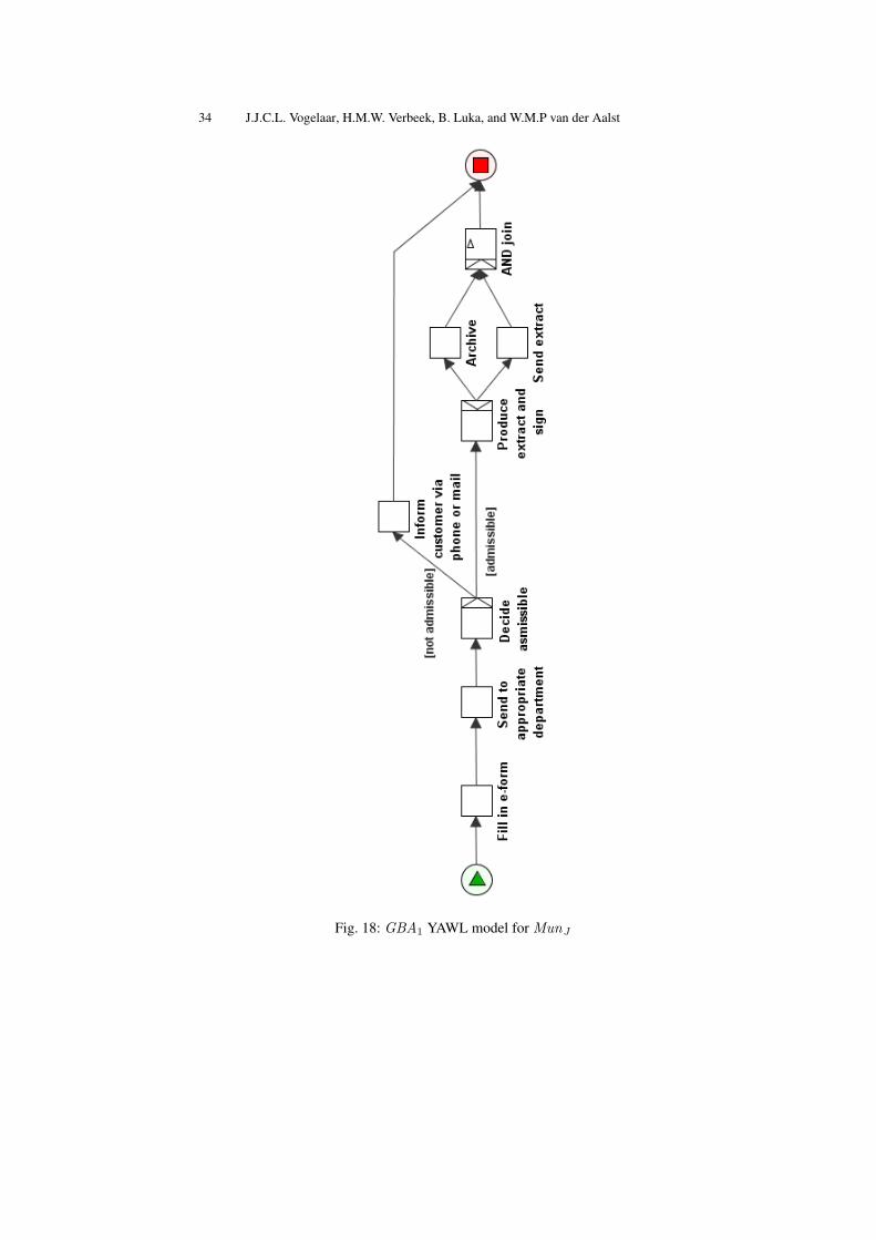
Fig. 18: GBA1 YAWL model for MunJ

Comparing Business Processes to Determine the Feasibility of Configurable Models 35

A.2 YAWL models for the GBA2 process

36 J.J.C.L. Vogelaar, H.M.W. Verbeek, B. Luka, and W.M.P van der Aalst

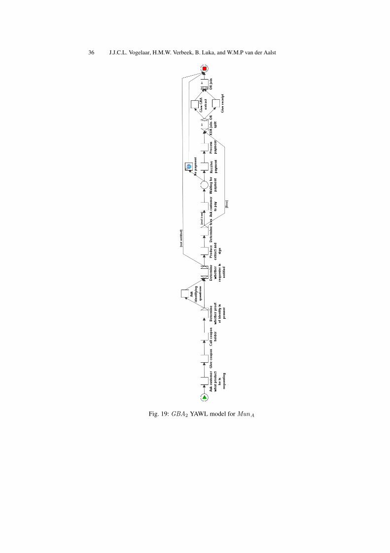
Fig. 19: GBA2 YAWL model for MunA

Comparing Business Processes to Determine the Feasibility of Configurable Models 37

Fig. 20: GBA2 YAWL model for MunB

38 J.J.C.L. Vogelaar, H.M.W. Verbeek, B. Luka, and W.M.P van der Aalst

Fig. 21: GBA2 YAWL model for MunC

Comparing Business Processes to Determine the Feasibility of Configurable Models 39

Fig. 22: GBA2 YAWL model for MunD

40 J.J.C.L. Vogelaar, H.M.W. Verbeek, B. Luka, and W.M.P van der Aalst

Fig. 23: GBA2 YAWL model for MunE

Comparing Business Processes to Determine the Feasibility of Configurable Models 41

Fig. 24: GBA2 YAWL model for MunF

42 J.J.C.L. Vogelaar, H.M.W. Verbeek, B. Luka, and W.M.P van der Aalst

Fig. 25: GBA2 YAWL model for MunG

Comparing Business Processes to Determine the Feasibility of Configurable Models 43

Fig. 26: GBA2 YAWL model for MunH

44 J.J.C.L. Vogelaar, H.M.W. Verbeek, B. Luka, and W.M.P van der Aalst

Fig. 27: GBA2 YAWL model for MunI

Comparing Business Processes to Determine the Feasibility of Configurable Models 45

Fig. 28: GBA2 YAWL model for MunJ

46 J.J.C.L. Vogelaar, H.M.W. Verbeek, B. Luka, and W.M.P van der Aalst

A.3 YAWL models for the GBA3 process

Comparing Business Processes to Determine the Feasibility of Configurable Models 47

Fig. 29: GBA3 YAWL model for MunA

48 J.J.C.L. Vogelaar, H.M.W. Verbeek, B. Luka, and W.M.P van der Aalst

Fig. 30: GBA3 YAWL model for MunB

Comparing Business Processes to Determine the Feasibility of Configurable Models 49

Fig. 31: GBA3 YAWL model for MunC

50 J.J.C.L. Vogelaar, H.M.W. Verbeek, B. Luka, and W.M.P van der Aalst

Fig. 32: GBA3 YAWL model for MunD

Comparing Business Processes to Determine the Feasibility of Configurable Models 51

Fig. 33: GBA3 YAWL model for MunE

52 J.J.C.L. Vogelaar, H.M.W. Verbeek, B. Luka, and W.M.P van der Aalst

Fig. 34: GBA3 YAWL model for MunF

Comparing Business Processes to Determine the Feasibility of Configurable Models 53

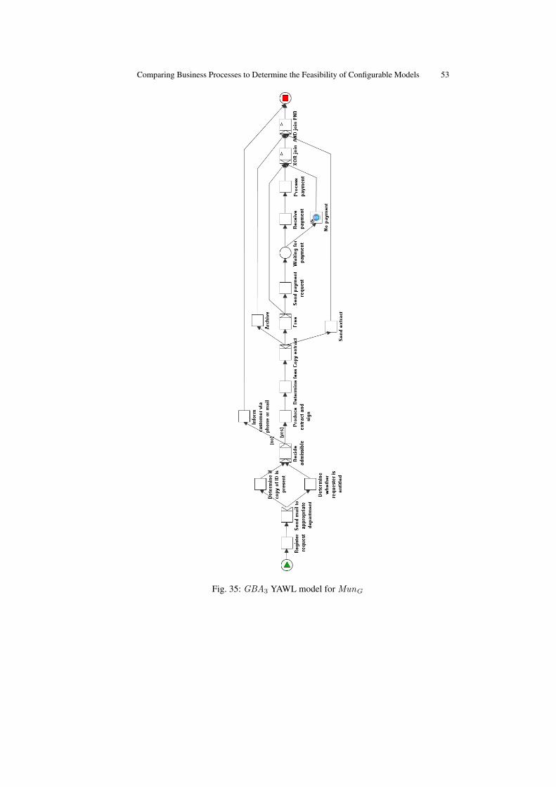
Fig. 35: GBA3 YAWL model for MunG

54 J.J.C.L. Vogelaar, H.M.W. Verbeek, B. Luka, and W.M.P van der Aalst

Fig. 36: GBA3 YAWL model for MunH

Comparing Business Processes to Determine the Feasibility of Configurable Models 55

Fig. 37: GBA3 YAWL model for MunI

56 J.J.C.L. Vogelaar, H.M.W. Verbeek, B. Luka, and W.M.P van der Aalst

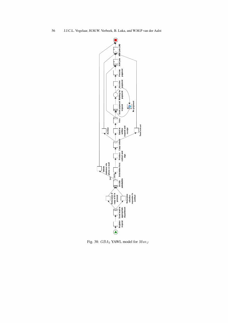
Fig. 38: GBA3 YAWL model for MunJ

Comparing Business Processes to Determine the Feasibility of Configurable Models 57

A.4 YAWL models for the MOR process

58 J.J.C.L. Vogelaar, H.M.W. Verbeek, B. Luka, and W.M.P van der Aalst

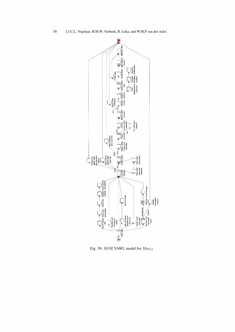
Fig. 39: MOR YAWL model for MunA

Comparing Business Processes to Determine the Feasibility of Configurable Models 59

Fig. 40: MOR YAWL model for MunB

60 J.J.C.L. Vogelaar, H.M.W. Verbeek, B. Luka, and W.M.P van der Aalst

Fig. 41: MOR YAWL model for MunC

Comparing Business Processes to Determine the Feasibility of Configurable Models 61

Fig. 42: MOR YAWL model for MunD

62 J.J.C.L. Vogelaar, H.M.W. Verbeek, B. Luka, and W.M.P van der Aalst

Fig. 43: MOR YAWL model for MunE

Comparing Business Processes to Determine the Feasibility of Configurable Models 63

Fig. 44: MOR YAWL model for MunF

64 J.J.C.L. Vogelaar, H.M.W. Verbeek, B. Luka, and W.M.P van der Aalst

Fig. 45: MOR YAWL model for MunG

Comparing Business Processes to Determine the Feasibility of Configurable Models 65

Fig. 46: MOR YAWL model for MunH

66 J.J.C.L. Vogelaar, H.M.W. Verbeek, B. Luka, and W.M.P van der Aalst

Fig. 47: MOR YAWL model for MunI

Comparing Business Processes to Determine the Feasibility of Configurable Models 67

Fig. 48: MOR YAWL model for MunJ

68 J.J.C.L. Vogelaar, H.M.W. Verbeek, B. Luka, and W.M.P van der Aalst

A.5 YAWL models for the WABO1 process

Comparing Business Processes to Determine the Feasibility of Configurable Models 69

Fig. 49: WABO1 YAWL model for MunA

70 J.J.C.L. Vogelaar, H.M.W. Verbeek, B. Luka, and W.M.P van der Aalst

Fig. 50: WABO1 YAWL model for MunB

Comparing Business Processes to Determine the Feasibility of Configurable Models 71

Fig. 51: WABO1 YAWL model for MunC

72 J.J.C.L. Vogelaar, H.M.W. Verbeek, B. Luka, and W.M.P van der Aalst

Fig. 52: WABO1 YAWL model for MunD

Comparing Business Processes to Determine the Feasibility of Configurable Models 73

Fig. 53: WABO1 YAWL model for MunE

74 J.J.C.L. Vogelaar, H.M.W. Verbeek, B. Luka, and W.M.P van der Aalst

Fig. 54: WABO1 YAWL model for MunF

Comparing Business Processes to Determine the Feasibility of Configurable Models 75

Fig. 55: WABO1 YAWL model for MunG

76 J.J.C.L. Vogelaar, H.M.W. Verbeek, B. Luka, and W.M.P van der Aalst

Fig. 56: WABO1 YAWL model for MunH

Comparing Business Processes to Determine the Feasibility of Configurable Models 77

Fig. 57: WABO1 YAWL model for MunI

78 J.J.C.L. Vogelaar, H.M.W. Verbeek, B. Luka, and W.M.P van der Aalst

Fig. 58: WABO1 YAWL model for MunJ

Comparing Business Processes to Determine the Feasibility of Configurable Models 79

A.6 YAWL models for the WABO2 process

80 J.J.C.L. Vogelaar, H.M.W. Verbeek, B. Luka, and W.M.P van der Aalst

Fig. 59: WABO2 YAWL model for MunA

Comparing Business Processes to Determine the Feasibility of Configurable Models 81

Fig. 60: WABO2 YAWL model for MunB

82 J.J.C.L. Vogelaar, H.M.W. Verbeek, B. Luka, and W.M.P van der Aalst

Fig. 61: WABO2 YAWL model for MunC

Comparing Business Processes to Determine the Feasibility of Configurable Models 83

Fig. 62: WABO2 YAWL model for MunD

84 J.J.C.L. Vogelaar, H.M.W. Verbeek, B. Luka, and W.M.P van der Aalst

Fig. 63: WABO2 YAWL model for MunE

Comparing Business Processes to Determine the Feasibility of Configurable Models 85

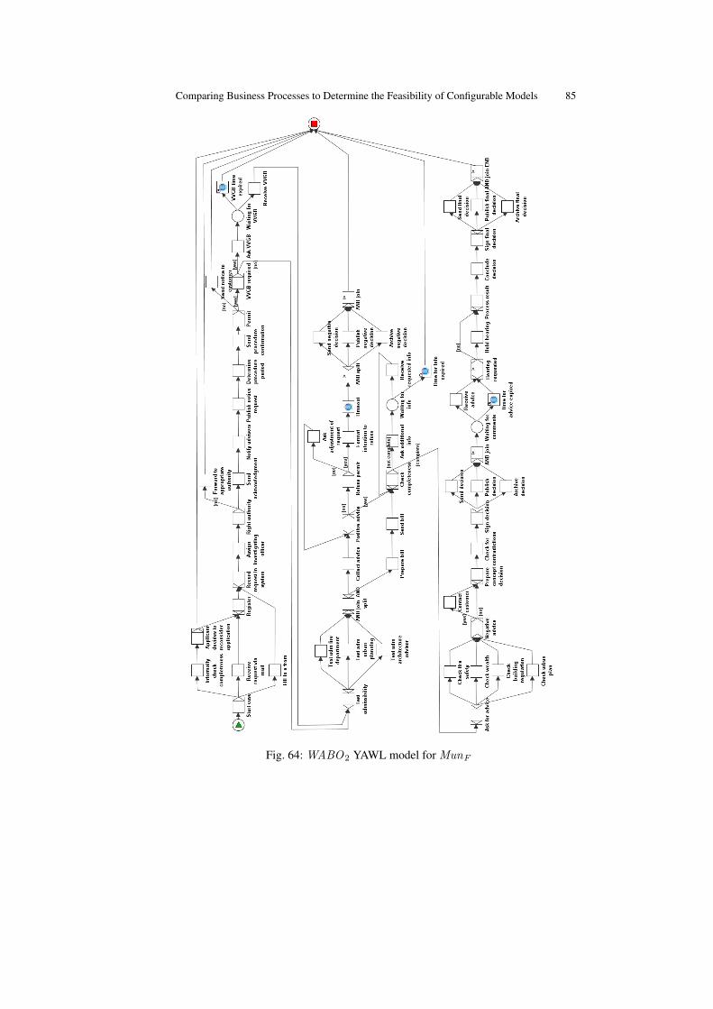
Fig. 64: WABO2 YAWL model for MunF

86 J.J.C.L. Vogelaar, H.M.W. Verbeek, B. Luka, and W.M.P van der Aalst

Fig. 65: WABO2 YAWL model for MunG

Comparing Business Processes to Determine the Feasibility of Configurable Models 87

Fig. 66: WABO2 YAWL model for MunH

88 J.J.C.L. Vogelaar, H.M.W. Verbeek, B. Luka, and W.M.P van der Aalst

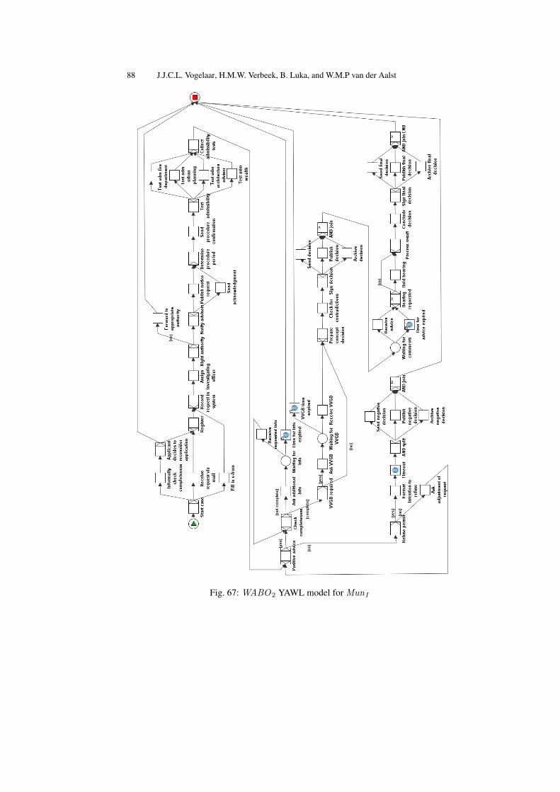
Fig. 67: WABO2 YAWL model for MunI

Comparing Business Processes to Determine the Feasibility of Configurable Models 89

Fig. 68: WABO2 YAWL model for MunJ

90 J.J.C.L. Vogelaar, H.M.W. Verbeek, B. Luka, and W.M.P van der Aalst

A.7 YAWL models for the WMO process

Fig. 69: WMO YAWL model for MunA

Comparing Business Processes to Determine the Feasibility of Configurable Models 91

Fig. 70: WMO YAWL model for MunB

92 J.J.C.L. Vogelaar, H.M.W. Verbeek, B. Luka, and W.M.P van der Aalst

Fig. 71: WMO YAWL model for MunC

Comparing Business Processes to Determine the Feasibility of Configurable Models 93

Fig. 72: WMO YAWL model for MunD

94 J.J.C.L. Vogelaar, H.M.W. Verbeek, B. Luka, and W.M.P van der Aalst

Fig. 73: WMO YAWL model for MunE

Comparing Business Processes to Determine the Feasibility of Configurable Models 95

Fig. 74: WMO YAWL model for MunF

96 J.J.C.L. Vogelaar, H.M.W. Verbeek, B. Luka, and W.M.P van der Aalst

Fig. 75: WMO YAWL model for MunG

Comparing Business Processes to Determine the Feasibility of Configurable Models 97

Fig. 76: WMO YAWL model for MunH

98 J.J.C.L. Vogelaar, H.M.W. Verbeek, B. Luka, and W.M.P van der Aalst

Fig. 77: WMO YAWL model for MunI

Comparing Business Processes to Determine the Feasibility of Configurable Models 99

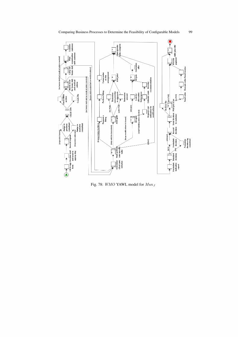
Fig. 78: WMO YAWL model for MunJ

100 J.J.C.L. Vogelaar, H.M.W. Verbeek, B. Luka, and W.M.P van der Aalst

A.8 YAWL models for the WOZ process

Comparing Business Processes to Determine the Feasibility of Configurable Models 101

Fig. 79: WOZ YAWL model for MunA

102 J.J.C.L. Vogelaar, H.M.W. Verbeek, B. Luka, and W.M.P van der Aalst

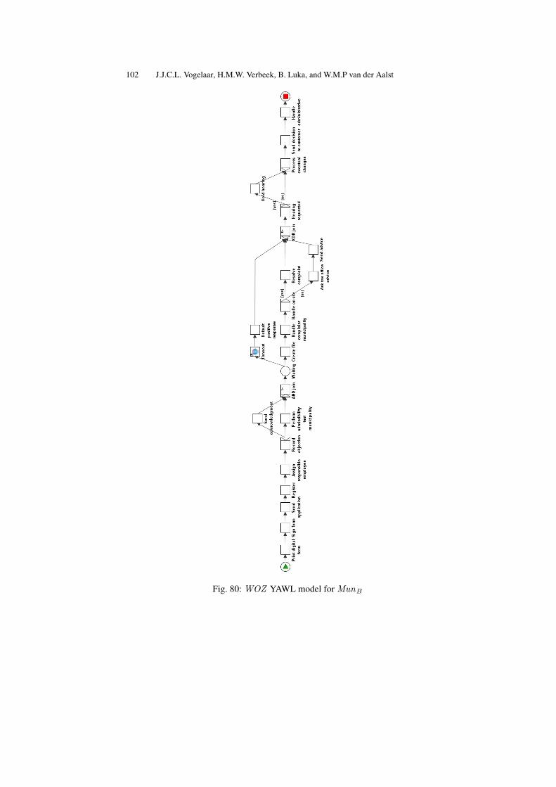
Fig. 80: WOZ YAWL model for MunB

Comparing Business Processes to Determine the Feasibility of Configurable Models 103

Fig. 81: WOZ YAWL model for MunC

104 J.J.C.L. Vogelaar, H.M.W. Verbeek, B. Luka, and W.M.P van der Aalst

Fig. 82: WOZ YAWL model for MunD

Comparing Business Processes to Determine the Feasibility of Configurable Models 105

Fig. 83: WOZ YAWL model for MunE

106 J.J.C.L. Vogelaar, H.M.W. Verbeek, B. Luka, and W.M.P van der Aalst

Fig. 84: WOZ YAWL model for MunF

Comparing Business Processes to Determine the Feasibility of Configurable Models 107

Fig. 85: WOZ YAWL model for MunG

108 J.J.C.L. Vogelaar, H.M.W. Verbeek, B. Luka, and W.M.P van der Aalst

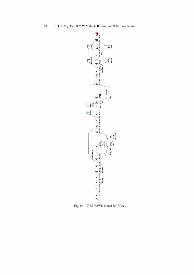
Fig. 86: WOZ YAWL model for MunH

Comparing Business Processes to Determine the Feasibility of Configurable Models 109

Fig. 87: WOZ YAWL model for MunI

110 J.J.C.L. Vogelaar, H.M.W. Verbeek, B. Luka, and W.M.P van der Aalst

Fig. 88: WOZ YAWL model for MunJ

Comparing Business Processes to Determine the Feasibility of Configurable Models 111

B Complexity results

B.1 GBA1 process

MunA MunB MunC MunD MunE MunF MunG MunH MunI MunJ

CFC 6 5 4 5 7 5 5 6 5 3Density 0.350 0.400 0.667 0.350 0.300 0.350 0.300 0.350 0.350 0.417

CC 0.078 0.205 0.172 0.167 0.108 0.180 0.117 0.078 0.180 0.184

B.2 GBA2 process

MunA MunB MunC MunD MunE MunF MunG MunH MunI MunJ

CFC 11 15 17 20 13 11 11 15 16 15Density 0.181 0.178 0.128 0.104 0.167 0.214 0.181 0.178 0.144 0.178

CC 0.045 0.037 0.030 0.030 0.039 0.048 0.045 0.037 0.030 0.037

B.3 GBA3 process

MunA MunB MunC MunD MunE MunF MunG MunH MunI MunJ

CFC 9 10 16 10 12 8 8 9 8 8Density 0.155 0.181 0.126 0.155 0.136 0.214 0.194 0.181 0.194 0.167

CC 0.079 0.075 0.054 0.080 0.067 0.120 0.113 0.074 0.113 0.109

B.4 MOR process

MunA MunB MunC MunD MunE MunF MunG MunH MunI MunJ

CFC 21 16 17 10 15 19 13 11 17 15Density 0.148 0.141 0.121 0.232 0.164 0.147 0.178 0.155 0.141 0.164

CC 0.027 0.032 0.027 0.051 0.032 0.028 0.036 0.047 0.032 0.032

B.5 WABO1 process

MunA MunB MunC MunD MunE MunF MunG MunH MunI MunJ

CFC 3 3 7 5 5 4 5 5 5 5Density 0.417 0.417 0.196 0.267 0.267 0.417 0.267 0.267 0.267 0.267

CC 0.160 0.271 0.076 0.110 0.094 0.100 0.094 0.094 0.094 0.094

B.6 WABO2 process

MunA MunB MunC MunD MunE MunF MunG MunH MunI MunJ

CFC 29 22 31 31 33 33 31 31 28 29Density 0.073 0.079 0.054 0.055 0.056 0.055 0.055 0.055 0.062 0.065

CC 0.036 0.043 0.033 0.034 0.029 0.029 0.034 0.034 0.039 0.030

112 J.J.C.L. Vogelaar, H.M.W. Verbeek, B. Luka, and W.M.P van der Aalst

B.7 WMO process

MunA MunB MunC MunD MunE MunF MunG MunH MunI MunJ

CFC 40 48 29 35 35 26 27 37 39 22Density 0.088 0.060 0.086 0.051 0.066 0.087 0.087 0.096 0.092 0.084

CC 0.018 0.018 0.026 0.025 0.022 0.031 0.025 0.021 0.021 0.029

B.8 WOZ process

MunA MunB MunC MunD MunE MunF MunG MunH MunI MunJ

CFC 10 7 11 10 20 13 12 10 10 17Density 0.136 0.238 0.096 0.136 0.088 0.110 0.115 0.155 0.155 0.092

CC 0.067 0.103 0.082 0.064 0.042 0.045 0.046 0.075 0.075 0.037

C Similarity results

C.1 GBA1 process

GED MunA MunB MunC MunD MunE MunF MunG MunH MunI MunJ

MunA 1.000 0.837 0.817 0.883 0.845 0.803 0.667 1.000 0.942 0.698MunB 0.837 1.000 0.772 0.915 0.841 0.842 0.708 0.837 0.896 0.769MunC 0.817 0.772 1.000 0.807 0.799 0.798 0.665 0.817 0.798 0.664MunD 0.883 0.915 0.807 1.000 0.884 0.891 0.719 0.883 0.950 0.801MunE 0.845 0.841 0.799 0.884 1.000 0.851 0.732 0.845 0.908 0.858MunF 0.803 0.842 0.798 0.891 0.851 1.000 0.711 0.803 0.879 0.793MunG 0.667 0.708 0.665 0.719 0.732 0.711 1.000 0.667 0.717 0.723MunH 1.000 0.837 0.817 0.883 0.845 0.803 0.667 1.000 0.942 0.698MunI 0.942 0.896 0.798 0.950 0.908 0.879 0.717 0.942 1.000 0.793MunJ 0.698 0.769 0.664 0.801 0.858 0.793 0.723 0.698 0.793 1.000

SPS MunA MunB MunC MunD MunE MunF MunG MunH MunI MunJ

MunA 1.000 0.573 0.813 0.741 0.622 0.649 0.250 1.000 0.788 0.289MunB 0.573 1.000 0.615 0.760 0.774 0.704 0.391 0.573 0.781 0.365MunC 0.813 0.615 1.000 0.768 0.600 0.739 0.200 0.813 0.735 0.304MunD 0.741 0.760 0.768 1.000 0.751 0.891 0.466 0.741 0.929 0.491MunE 0.622 0.774 0.600 0.751 1.000 0.757 0.372 0.622 0.802 0.538MunF 0.649 0.704 0.739 0.891 0.757 1.000 0.364 0.649 0.917 0.483MunG 0.250 0.391 0.200 0.466 0.372 0.364 1.000 0.250 0.359 0.525MunH 1.000 0.573 0.813 0.741 0.622 0.649 0.250 1.000 0.788 0.289MunI 0.788 0.781 0.735 0.929 0.802 0.917 0.359 0.788 1.000 0.459MunJ 0.289 0.365 0.304 0.491 0.538 0.483 0.525 0.289 0.459 1.000

Comparing Business Processes to Determine the Feasibility of Configurable Models 113

C.2 GBA2 process

GED MunA MunB MunC MunD MunE MunF MunG MunH MunI MunJ

MunA 1.000 0.898 0.867 0.811 0.957 0.962 0.980 0.898 0.891 0.898MunB 0.898 1.000 0.919 0.897 0.944 0.932 0.894 1.000 0.911 1.000MunC 0.867 0.919 1.000 0.840 0.898 0.863 0.867 0.919 0.845 0.919MunD 0.811 0.897 0.840 1.000 0.851 0.838 0.806 0.897 0.827 0.897MunE 0.957 0.944 0.898 0.851 1.000 0.938 0.937 0.944 0.924 0.944MunF 0.962 0.932 0.863 0.838 0.938 1.000 0.941 0.932 0.901 0.932MunG 0.980 0.894 0.867 0.806 0.937 0.941 1.000 0.894 0.890 0.894MunH 0.898 1.000 0.919 0.897 0.944 0.932 0.894 1.000 0.911 1.000MunI 0.891 0.911 0.845 0.827 0.924 0.901 0.890 0.911 1.000 0.911MunJ 0.898 1.000 0.919 0.897 0.944 0.932 0.894 1.000 0.911 1.000

SPS MunA MunB MunC MunD MunE MunF MunG MunH MunI MunJ

MunA 1.000 0.756 0.526 0.472 0.889 0.942 0.970 0.756 0.710 0.756MunB 0.756 1.000 0.747 0.628 0.858 0.784 0.736 1.000 0.792 1.000MunC 0.526 0.747 1.000 0.523 0.628 0.475 0.526 0.747 0.557 0.747MunD 0.472 0.628 0.523 1.000 0.540 0.494 0.463 0.628 0.488 0.628MunE 0.889 0.858 0.628 0.540 1.000 0.837 0.863 0.858 0.830 0.858MunF 0.942 0.784 0.475 0.494 0.837 1.000 0.912 0.784 0.713 0.784MunG 0.970 0.736 0.526 0.463 0.863 0.912 1.000 0.736 0.691 0.736MunH 0.756 1.000 0.747 0.628 0.858 0.784 0.736 1.000 0.792 1.000MunI 0.710 0.792 0.557 0.488 0.830 0.713 0.691 0.792 1.000 0.792MunJ 0.756 1.000 0.747 0.628 0.858 0.784 0.736 1.000 0.792 1.000

C.3 GBA3 process

GED MunA MunB MunC MunD MunE MunF MunG MunH MunI MunJ

MunA 1.000 0.758 0.735 0.762 0.788 0.796 0.779 0.765 0.779 0.793MunB 0.758 1.000 0.749 0.759 0.782 0.779 0.776 0.741 0.776 0.801MunC 0.735 0.749 1.000 0.764 0.799 0.793 0.770 0.733 0.770 0.804MunD 0.762 0.759 0.764 1.000 0.823 0.841 0.911 0.762 0.911 0.837MunE 0.788 0.782 0.799 0.823 1.000 0.874 0.848 0.786 0.848 0.882MunF 0.796 0.779 0.793 0.841 0.874 1.000 0.875 0.793 0.875 0.868MunG 0.779 0.776 0.770 0.911 0.848 0.875 1.000 0.777 1.000 0.870MunH 0.765 0.741 0.733 0.762 0.786 0.793 0.777 1.000 0.777 0.829MunI 0.779 0.776 0.770 0.911 0.848 0.875 1.000 0.777 1.000 0.870MunJ 0.793 0.801 0.804 0.837 0.882 0.868 0.870 0.829 0.870 1.000

114 J.J.C.L. Vogelaar, H.M.W. Verbeek, B. Luka, and W.M.P van der Aalst

SPS MunA MunB MunC MunD MunE MunF MunG MunH MunI MunJ

MunA 1.000 0.495 0.426 0.543 0.559 0.617 0.569 0.650 0.569 0.581MunB 0.495 1.000 0.405 0.494 0.406 0.595 0.639 0.475 0.639 0.634MunC 0.426 0.405 1.000 0.564 0.563 0.295 0.504 0.408 0.504 0.633MunD 0.543 0.494 0.564 1.000 0.503 0.529 0.789 0.637 0.789 0.698MunE 0.559 0.406 0.563 0.503 1.000 0.376 0.549 0.403 0.549 0.500MunF 0.617 0.595 0.295 0.529 0.376 1.000 0.660 0.584 0.660 0.616MunG 0.569 0.639 0.504 0.789 0.549 0.660 1.000 0.735 1.000 0.888MunH 0.650 0.475 0.408 0.637 0.403 0.584 0.735 1.000 0.735 0.755MunI 0.569 0.639 0.504 0.789 0.549 0.660 1.000 0.735 1.000 0.888MunJ 0.581 0.634 0.633 0.698 0.500 0.616 0.888 0.755 0.888 1.000

C.4 MOR process

GED MunA MunB MunC MunD MunE MunF MunG MunH MunI MunJ

MunA 1.000 0.832 0.773 0.763 0.837 0.738 0.801 0.743 0.766 0.757MunB 0.832 1.000 0.785 0.790 0.858 0.767 0.820 0.755 0.774 0.778MunC 0.773 0.785 1.000 0.739 0.860 0.737 0.804 0.739 0.740 0.739MunD 0.763 0.790 0.739 1.000 0.796 0.741 0.789 0.758 0.742 0.754MunE 0.837 0.858 0.860 0.796 1.000 0.767 0.895 0.770 0.781 0.775MunF 0.738 0.767 0.737 0.741 0.767 1.000 0.779 0.733 0.733 0.803MunG 0.801 0.820 0.804 0.789 0.895 0.779 1.000 0.768 0.738 0.812MunH 0.743 0.755 0.739 0.758 0.770 0.733 0.768 1.000 0.729 0.757MunI 0.766 0.774 0.740 0.742 0.781 0.733 0.738 0.729 1.000 0.721MunJ 0.757 0.778 0.739 0.754 0.775 0.803 0.812 0.757 0.721 1.000

SPS MunA MunB MunC MunD MunE MunF MunG MunH MunI MunJ

MunA 1.000 0.603 0.509 0.419 0.533 0.530 0.544 0.359 0.367 0.421MunB 0.603 1.000 0.540 0.595 0.624 0.573 0.547 0.579 0.434 0.418MunC 0.509 0.540 1.000 0.470 0.709 0.449 0.631 0.437 0.299 0.524MunD 0.419 0.595 0.470 1.000 0.489 0.443 0.478 0.503 0.457 0.467MunE 0.533 0.624 0.709 0.489 1.000 0.475 0.864 0.504 0.498 0.519MunF 0.530 0.573 0.449 0.443 0.475 1.000 0.539 0.523 0.470 0.581MunG 0.544 0.547 0.631 0.478 0.864 0.539 1.000 0.556 0.427 0.683MunH 0.359 0.579 0.437 0.503 0.504 0.523 0.556 1.000 0.377 0.470MunI 0.367 0.434 0.299 0.457 0.498 0.470 0.427 0.377 1.000 0.351MunJ 0.421 0.418 0.524 0.467 0.519 0.581 0.683 0.470 0.351 1.000

Comparing Business Processes to Determine the Feasibility of Configurable Models 115

C.5 WABO1 process

GED MunA MunB MunC MunD MunE MunF MunG MunH MunI MunJ

MunA 1.000 0.682 0.656 0.656 0.769 0.657 0.769 0.769 0.769 0.769MunB 0.682 1.000 0.748 0.794 0.794 0.765 0.794 0.794 0.794 0.794MunC 0.656 0.748 1.000 0.850 0.819 0.784 0.819 0.819 0.819 0.819MunD 0.656 0.794 0.850 1.000 0.952 0.878 0.952 0.952 0.952 0.952MunE 0.769 0.794 0.819 0.952 1.000 0.878 1.000 1.000 1.000 1.000MunF 0.657 0.765 0.784 0.878 0.878 1.000 0.878 0.878 0.878 0.878MunG 0.769 0.794 0.819 0.952 1.000 0.878 1.000 1.000 1.000 1.000MunH 0.769 0.794 0.819 0.952 1.000 0.878 1.000 1.000 1.000 1.000MunI 0.769 0.794 0.819 0.952 1.000 0.878 1.000 1.000 1.000 1.000MunJ 0.769 0.794 0.819 0.952 1.000 0.878 1.000 1.000 1.000 1.000

SPS MunA MunB MunC MunD MunE MunF MunG MunH MunI MunJ

MunA 1.000 0.303 0.539 0.629 0.681 0.565 0.681 0.681 0.681 0.681MunB 0.303 1.000 0.416 0.488 0.488 0.513 0.488 0.488 0.488 0.488MunC 0.539 0.416 1.000 0.775 0.728 0.574 0.728 0.728 0.728 0.728MunD 0.629 0.488 0.775 1.000 0.948 0.784 0.948 0.948 0.948 0.948MunE 0.681 0.488 0.728 0.948 1.000 0.778 1.000 1.000 1.000 1.000MunF 0.565 0.513 0.574 0.784 0.778 1.000 0.778 0.778 0.778 0.778MunG 0.681 0.488 0.728 0.948 1.000 0.778 1.000 1.000 1.000 1.000MunH 0.681 0.488 0.728 0.948 1.000 0.778 1.000 1.000 1.000 1.000MunI 0.681 0.488 0.728 0.948 1.000 0.778 1.000 1.000 1.000 1.000MunJ 0.681 0.488 0.728 0.948 1.000 0.778 1.000 1.000 1.000 1.000

C.6 WABO2 process

GED MunA MunB MunC MunD MunE MunF MunG MunH MunI MunJ

MunA 1.000 0.787 0.830 0.872 0.836 0.833 0.872 0.872 0.840 0.789MunB 0.787 1.000 0.728 0.728 0.724 0.725 0.728 0.728 0.736 0.734MunC 0.830 0.728 1.000 0.925 0.905 0.903 0.925 0.925 0.917 0.880MunD 0.872 0.728 0.925 1.000 0.944 0.943 1.000 1.000 0.969 0.901MunE 0.836 0.724 0.905 0.944 1.000 0.996 0.944 0.944 0.917 0.904MunF 0.833 0.725 0.903 0.943 0.996 1.000 0.943 0.943 0.915 0.907MunG 0.872 0.728 0.925 1.000 0.944 0.943 1.000 1.000 0.969 0.901MunH 0.872 0.728 0.925 1.000 0.944 0.943 1.000 1.000 0.969 0.901MunI 0.840 0.736 0.917 0.969 0.917 0.915 0.969 0.969 1.000 0.906MunJ 0.789 0.734 0.880 0.901 0.904 0.907 0.901 0.901 0.906 1.000

116 J.J.C.L. Vogelaar, H.M.W. Verbeek, B. Luka, and W.M.P van der Aalst

SPS MunA MunB MunC MunD MunE MunF MunG MunH MunI MunJ

MunA 1.000 0.500 0.700 0.776 0.596 0.582 0.776 0.776 0.711 0.505MunB 0.500 1.000 0.445 0.416 0.471 0.443 0.416 0.416 0.328 0.273MunC 0.700 0.445 1.000 0.887 0.746 0.733 0.887 0.887 0.766 0.548MunD 0.776 0.416 0.887 1.000 0.787 0.778 1.000 1.000 0.889 0.617MunE 0.596 0.471 0.746 0.787 1.000 0.986 0.787 0.787 0.682 0.689MunF 0.582 0.443 0.733 0.778 0.986 1.000 0.778 0.778 0.669 0.695MunG 0.776 0.416 0.887 1.000 0.787 0.778 1.000 1.000 0.889 0.617MunH 0.776 0.416 0.887 1.000 0.787 0.778 1.000 1.000 0.889 0.617MunI 0.711 0.328 0.766 0.889 0.682 0.669 0.889 0.889 1.000 0.732MunJ 0.505 0.273 0.548 0.617 0.689 0.695 0.617 0.617 0.732 1.000

C.7 WMO process

GED MunA MunB MunC MunD MunE MunF MunG MunH MunI MunJ

MunA 1.000 0.916 0.817 0.773 0.776 0.802 0.795 0.976 0.949 0.801MunB 0.916 1.000 0.791 0.755 0.758 0.778 0.773 0.927 0.901 0.777MunC 0.817 0.791 1.000 0.758 0.831 0.816 0.858 0.825 0.813 0.821MunD 0.773 0.755 0.758 1.000 0.746 0.759 0.745 0.779 0.778 0.757MunE 0.776 0.758 0.831 0.746 1.000 0.785 0.804 0.781 0.780 0.784MunF 0.802 0.778 0.816 0.759 0.785 1.000 0.807 0.809 0.797 0.811MunG 0.795 0.773 0.858 0.745 0.804 0.807 1.000 0.802 0.790 0.805MunH 0.976 0.927 0.825 0.779 0.781 0.809 0.802 1.000 0.966 0.809MunI 0.949 0.901 0.813 0.778 0.780 0.797 0.790 0.966 1.000 0.797MunJ 0.801 0.777 0.821 0.757 0.784 0.811 0.805 0.809 0.797 1.000

SPS MunA MunB MunC MunD MunE MunF MunG MunH MunI MunJ

MunA 1.000 0.694 0.515 0.432 0.497 0.431 0.423 0.923 0.893 0.512MunB 0.694 1.000 0.367 0.372 0.400 0.359 0.388 0.669 0.656 0.404MunC 0.515 0.367 1.000 0.348 0.601 0.536 0.616 0.452 0.469 0.584MunD 0.432 0.372 0.348 1.000 0.336 0.354 0.264 0.449 0.435 0.373MunE 0.497 0.400 0.601 0.336 1.000 0.476 0.511 0.398 0.440 0.470MunF 0.431 0.359 0.536 0.354 0.476 1.000 0.433 0.462 0.491 0.565MunG 0.423 0.388 0.616 0.264 0.511 0.433 1.000 0.420 0.432 0.457MunH 0.923 0.669 0.452 0.449 0.398 0.462 0.420 1.000 0.930 0.548MunI 0.893 0.656 0.469 0.435 0.440 0.491 0.432 0.930 1.000 0.529MunJ 0.512 0.404 0.584 0.373 0.470 0.565 0.457 0.548 0.529 1.000

Comparing Business Processes to Determine the Feasibility of Configurable Models 117

C.8 WOZ process

GED MunA MunB MunC MunD MunE MunF MunG MunH MunI MunJ

MunA 1.000 0.916 0.817 0.773 0.776 0.802 0.795 0.976 0.949 0.801MunB 0.916 1.000 0.791 0.755 0.758 0.778 0.773 0.927 0.901 0.777MunC 0.817 0.791 1.000 0.758 0.831 0.816 0.858 0.825 0.813 0.821MunD 0.773 0.755 0.758 1.000 0.746 0.759 0.745 0.779 0.778 0.757MunE 0.776 0.758 0.831 0.746 1.000 0.785 0.804 0.781 0.780 0.784MunF 0.802 0.778 0.816 0.759 0.785 1.000 0.807 0.809 0.797 0.811MunG 0.795 0.773 0.858 0.745 0.804 0.807 1.000 0.802 0.790 0.805MunH 0.976 0.927 0.825 0.779 0.781 0.809 0.802 1.000 0.966 0.809MunI 0.949 0.901 0.813 0.778 0.780 0.797 0.790 0.966 1.000 0.797MunJ 0.801 0.777 0.821 0.757 0.784 0.811 0.805 0.809 0.797 1.000

SPS MunA MunB MunC MunD MunE MunF MunG MunH MunI MunJ

MunA 1.000 0.389 0.511 0.549 0.395 0.499 0.531 0.487 0.487 0.466MunB 0.389 1.000 0.491 0.431 0.413 0.435 0.425 0.592 0.592 0.416MunC 0.511 0.491 1.000 0.437 0.380 0.441 0.482 0.527 0.527 0.364MunD 0.549 0.431 0.437 1.000 0.540 0.672 0.673 0.809 0.809 0.562MunE 0.395 0.413 0.380 0.540 1.000 0.596 0.516 0.666 0.666 0.812MunF 0.499 0.435 0.441 0.672 0.596 1.000 0.879 0.744 0.744 0.649MunG 0.531 0.425 0.482 0.673 0.516 0.879 1.000 0.658 0.658 0.563MunH 0.487 0.592 0.527 0.809 0.666 0.744 0.658 1.000 1.000 0.563MunI 0.487 0.592 0.527 0.809 0.666 0.744 0.658 1.000 1.000 0.687MunJ 0.466 0.416 0.364 0.562 0.812 0.649 0.563 0.563 0.687 1.000

118 J.J.C.L. Vogelaar, H.M.W. Verbeek, B. Luka, and W.M.P van der Aalst

D Similary vs. complexity

Process Mun1 Mun2 GED SPS Unified CFC Density CC Unified

GBA1 MunA MunG 0.667 0.250 0.258 51 0.087 0.020 39GBA1 MunC MunG 0.665 0.200 0.232 33 0.095 0.023 30GBA1 MunC MunI 0.798 0.735 0.638 15 0.194 0.049 13GBA1 MunD MunG 0.719 0.466 0.422 36 0.095 0.019 33GBA1 MunD MunI 0.950 0.929 0.894 7 0.238 0.091 7GBA1 MunE MunB 0.841 0.774 0.702 15 0.232 0.044 13GBA1 MunF MunH 0.803 0.649 0.601 13 0.167 0.043 13GBA1 MunG MunF 0.711 0.364 0.362 34 0.108 0.026 28GBA1 MunH MunB 0.837 0.573 0.598 17 0.178 0.048 14GBA1 MunI MunA 0.942 0.788 0.815 11 0.214 0.061 10GBA1 MunI MunB 0.896 0.781 0.763 13 0.262 0.047 11GBA1 MunI MunF 0.879 0.917 0.814 7 0.238 0.084 7GBA1 MunJ MunD 0.801 0.491 0.519 9 0.214 0.072 9GBA1 MunJ MunI 0.793 0.459 0.495 9 0.214 0.073 9

GBA2 MunA MunB 0.898 0.756 0.754 20 0.114 0.023 24GBA2 MunA MunC 0.867 0.526 0.606 27 0.084 0.018 32GBA2 MunC MunG 0.867 0.526 0.606 25 0.088 0.021 29GBA2 MunE MunF 0.938 0.837 0.835 16 0.144 0.029 18GBA2 MunE MunJ 0.944 0.858 0.852 18 0.135 0.028 20GBA2 MunF MunC 0.863 0.574 0.625 26 0.091 0.018 31GBA2 MunF MunG 0.941 0.912 0.876 12 0.167 0.034 15GBA2 MunF MunH 0.932 0.784 0.803 19 0.121 0.025 22GBA2 MunG MunJ 0.894 0.736 0.739 18 0.121 0.025 22GBA2 MunH MunD 0.897 0.628 0.688 33 0.083 0.021 32GBA2 MunI MunA 0.891 0.710 0.723 19 0.121 0.025 22GBA2 MunI MunD 0.827 0.488 0.545 39 0.063 0.016 43GBA2 MunI MunE 0.924 0.830 0.817 19 0.110 0.023 24GBA2 MunJ MunE 0.944 0.858 0.852 18 0.135 0.028 20

GBA3 MunA MunB 0.758 0.495 0.477 38 0.078 0.031 30GBA3 MunA MunF 0.796 0.617 0.577 30 0.071 0.027 30GBA3 MunB MunH 0.741 0.475 0.449 37 0.069 0.018 39GBA3 MunC MunG 0.770 0.504 0.493 30 0.069 0.019 35GBA3 MunD MunE 0.823 0.503 0.548 28 0.081 0.027 28GBA3 MunD MunF 0.841 0.529 0.581 33 0.068 0.022 34GBA3 MunE MunJ 0.882 0.698 0.708 25 0.103 0.035 22GBA3 MunF MunC 0.793 0.295 0.413 33 0.063 0.021 36GBA3 MunG MunB 0.776 0.639 0.567 29 0.081 0.028 28GBA3 MunG MunD 0.911 0.789 0.784 17 0.124 0.052 15GBA3 MunG MunI 1.000 1.000 0.982 8 0.194 0.113 7GBA3 MunI MunF 0.875 0.660 0.681 30 0.078 0.026 29GBA3 MunJ MunB 0.801 0.634 0.590 26 0.081 0.033 25GBA3 MunJ MunE 0.882 0.500 0.609 25 0.103 0.035 22

MOR MunA MunC 0.773 0.509 0.499 42 0.067 0.012 50MOR MunC MunA 0.773 0.509 0.499 42 0.067 0.012 50MOR MunC MunE 0.860 0.709 0.690 31 0.073 0.015 39MOR MunC MunJ 0.739 0.524 0.471 40 0.062 0.012 49MOR MunD MunJ 0.754 0.467 0.458 29 0.080 0.016 36MOR MunE MunF 0.767 0.475 0.476 45 0.057 0.011 56MOR MunE MunH 0.770 0.504 0.493 32 0.066 0.017 38

Comparing Business Processes to Determine the Feasibility of Configurable Models 119

Process Mun1 Mun2 GED SPS Unified CFC Density CC Unified

MOR MunF MunE 0.767 0.475 0.476 45 0.057 0.011 55MOR MunG MunE 0.895 0.864 0.804 27 0.096 0.021 29MOR MunH MunC 0.739 0.437 0.427 37 0.055 0.013 48MOR MunH MunG 0.768 0.556 0.517 32 0.066 0.017 39MOR MunH MunJ 0.757 0.470 0.463 34 0.060 0.015 44MOR MunI MunC 0.740 0.299 0.359 36 0.075 0.014 43MOR MunJ MunH 0.757 0.470 0.463 34 0.060 0.015 44

WABO1 MunA MunI 0.769 0.681 0.581 12 0.100 0.044 16WABO1 MunB MunC 0.748 0.416 0.427 18 0.076 0.032 23WABO1 MunB MunG 0.794 0.488 0.511 14 0.096 0.037 19WABO1 MunD MunB 0.794 0.488 0.511 14 0.096 0.039 18WABO1 MunD MunI 0.952 0.948 0.906 10 0.129 0.065 12WABO1 MunE MunH 1.000 1.000 0.982 5 0.267 0.094 6WABO1 MunE MunJ 1.000 1.000 0.982 5 0.267 0.094 6WABO1 MunG MunD 0.952 0.948 0.906 10 0.129 0.065 12WABO1 MunG MunE 1.000 1.000 0.982 5 0.267 0.094 6WABO1 MunI MunE 1.000 1.000 0.982 5 0.267 0.094 6WABO1 MunJ MunA 0.769 0.681 0.581 12 0.100 0.044 16WABO1 MunJ MunE 1.000 1.000 0.982 5 0.267 0.094 6WABO1 MunJ MunF 0.878 0.778 0.743 15 0.105 0.037 18

WABO2 MunA MunG 0.872 0.776 0.736 130 0.036 0.012 92WABO2 MunA MunH 0.872 0.776 0.736 130 0.036 0.012 92WABO2 MunD MunC 0.925 0.887 0.846 70 0.032 0.015 71WABO2 MunE MunA 0.836 0.596 0.608 144 0.032 0.012 103WABO2 MunH MunF 0.943 0.778 0.811 63 0.043 0.020 55WABO2 MunI MunF 0.915 0.669 0.728 63 0.044 0.020 54WABO2 MunJ MunC 0.880 0.548 0.631 65 0.031 0.014 72WABO2 MunJ MunG 0.901 0.617 0.687 55 0.032 0.017 64WABO2 MunJ MunI 0.906 0.732 0.749 44 0.042 0.021 48

WMO MunA MunD 0.773 0.432 0.461 100 0.026 0.009 107WMO MunA MunE 0.776 0.497 0.496 80 0.033 0.009 88WMO MunC MunB 0.791 0.367 0.446 71 0.038 0.012 73WMO MunC MunH 0.825 0.452 0.525 60 0.049 0.012 62WMO MunD MunA 0.773 0.432 0.461 99 0.026 0.009 105WMO MunE MunA 0.776 0.497 0.496 83 0.032 0.008 93WMO MunE MunB 0.758 0.400 0.429 89 0.029 0.009 96WMO MunE MunC 0.831 0.601 0.606 82 0.032 0.009 92WMO MunE MunJ 0.784 0.470 0.491 68 0.035 0.011 75WMO MunF MunA 0.802 0.431 0.490 67 0.043 0.010 72WMO MunF MunE 0.785 0.476 0.496 62 0.038 0.011 71WMO MunG MunJ 0.805 0.457 0.507 61 0.046 0.012 62WMO MunJ MunD 0.757 0.373 0.414 83 0.028 0.013 84WMO MunJ MunF 0.811 0.565 0.566 59 0.040 0.011 70

WOZ MunA MunC 0.771 0.511 0.498 48 0.045 0.018 50WOZ MunB MunI 0.745 0.592 0.511 51 0.056 0.015 51WOZ MunC MunD 0.736 0.437 0.425 50 0.046 0.018 50WOZ MunD MunG 0.831 0.673 0.641 27 0.058 0.019 37WOZ MunE MunF 0.799 0.596 0.570 35 0.045 0.016 48WOZ MunE MunI 0.895 0.666 0.704 30 0.058 0.020 37WOZ MunF MunE 0.799 0.596 0.570 35 0.045 0.016 48WOZ MunJ MunE 0.875 0.812 0.757 41 0.046 0.016 49

120 J.J.C.L. Vogelaar, H.M.W. Verbeek, B. Luka, and W.M.P van der Aalst

E Clusters

Cluster GBA1 GBA2 GBA3 MOR WABO1 WABO2 WMO WOZ

BDEFI D DFH DHI F CDGHI D DEHIJk GJ AEFGI GIJ BEFGJ DEGHIJ AB CEFGJ AFG

C BCHJ ABCE AC ABC EFJ ABHI BC

AF BDEJ CEG BDE DEH DH AEGI F1 G I ABDI ACGH AFIJ FIJ DFJ AGH

BCDEHIJ ACFGH FHJ FIJ BCG ABCEG BCH BCDEIJ

AJ ACDE EIJ H BDGHIJ G CE BCG2 BDGH BI BD ACGI CEF CFH BFGHIJ AEFIJ

CEFI FGHJ ACFGH BDEFJ A ABDEIJ AD DH

EIJ BCEG CEG F CG ADHIJ ACDE DJ3 ACFH ADF AHJ CDG ABDJ EFG BFGHJ EFI

BDG HIJ BDFI ABEHIJ EFHI BC I ABCGH

CEFI CDH BEIJ BCD G AG ABCIJ BCJ4 BJ ABG AFH AFGI ACDEFHJBCDEFIJ H FGH

ADGH EFIJ CDG EHJ BI H DEFG ADEI

E ABC BH CDGIJ B BCDEGIJ E CEIJ5 CFHJ FGIJ ACG ABEH ACDEF AH BI ABDF

ABDGI DEH DEFIJ F GHIJ F ACDFGHJ GH

ABCF ACDH EHJ BCHI BDH BH AEH ACHI6 DEIJ BEIJ BD DEF CEIJ AEGJ J BDEGJ

GH FG ACFGI AGJ AFG CDFI BCDFGI F

F BGHI CEGJ E CEI DEHI BCFI ABDEFGJ7 BCDH CF ABFHI ABDIJ DFGJ FG AEJ H

AEGIJ ADEJ D CGH ABH ABCJ DGH CI

CEFIJ ACJ BEH ACFJ ACG AGHI CDFG AEI8 BG EH ADFG BDI BDEHIJ BDF EI BCDGH

ADH BDFGI CIJ EGH F CEJ ABHJ FJ

AEGJ ADGJ ADG AIJ J BCDE ABCEF ABFIJ9 CH EF BCFH BCDEF ACDFGI AF IJ EGH

BDFI BCHI EIJ GH BEH GHIJ DGH CD

BCDGI FI FHIJ FGJ DHI CEFGIJ AEGJ E10 FH AJ ACE BEH AE AB BDH ABCFGHI

AEJ BCDEGH BDG ACDI BCFGJ DH CFI DJ