sensors

Article

Comparing RIEGL RiCOPTER UAV LiDAR DerivedCanopy Height and DBH with Terrestrial LiDAR

Benjamin Brede 1,* ID , Alvaro Lau 1,2 ID , Harm M. Bartholomeus 1 and Lammert Kooistra 1

1 Laboratory of Geo-Information Science and Remote Sensing, Wageningen University & Research,Droevendaalsesteeg, 36708 PB Wageningen, The Netherlands; alvaro.lausarmiento@wur.nl (A.L.);harm.bartholomeus@wur.nl (H.M.B.); lammert.kooistra@wur.nl (L.K.)

2 Center for International Forestry Research (CIFOR), Situ Gede, Sindang Barang, Bogor 16680, Indonesia* Correspondence: benjamin.brede@wur.nl (B.B.)

Received: 15 August 2017; Accepted: 13 October 2017; Published: 17 October 2017

Abstract: In recent years, LIght Detection And Ranging (LiDAR) and especially Terrestrial LaserScanning (TLS) systems have shown the potential to revolutionise forest structural characterisationby providing unprecedented 3D data. However, manned Airborne Laser Scanning (ALS) requirescostly campaigns and produces relatively low point density, while TLS is labour intense and timedemanding. Unmanned Aerial Vehicle (UAV)-borne laser scanning can be the way in between. In thisstudy, we present first results and experiences with the RIEGL RiCOPTER with VUX R©-1UAV ALSsystem and compare it with the well tested RIEGL VZ-400 TLS system. We scanned the same forestplots with both systems over the course of two days. We derived Digital Terrain Models (DTMs),Digital Surface Models (DSMs) and finally Canopy Height Models (CHMs) from the resulting pointclouds. ALS CHMs were on average 11.5 cm higher in five plots with different canopy conditions.This showed that TLS could not always detect the top of canopy. Moreover, we extracted trunksegments of 58 trees for ALS and TLS simultaneously, of which 39 could be used to model Diameterat Breast Height (DBH). ALS DBH showed a high agreement with TLS DBH with a correlationcoefficient of 0.98 and root mean square error of 4.24 cm. We conclude that RiCOPTER has thepotential to perform comparable to TLS for estimating forest canopy height and DBH under thestudied forest conditions. Further research should be directed to testing UAV-borne LiDAR forexplicit 3D modelling of whole trees to estimate tree volume and subsequently Above-GroundBiomass (AGB).

Keywords: UAV; LiDAR; ALS; TLS; forest inventory

1. Introduction

LIght Detection And Ranging (LiDAR) has become a valuable source of information to assessvegetation canopy structure. This is especially true for complex forest canopies that limit manualand destructive sampling. These capabilities are investigated to replace traditional forest plotinventories [1], but even more if they can deliver additional information that is not captured withtraditional inventories [2]. One particular important variable in this context is Above-Ground Biomass(AGB) which makes up an essential part of the forest carbon pool. Terrestrial Laser Scanning (TLS) hasthe potential to accurately measure AGB on a plot scale [3,4], while Airborne Laser Scanning (ALS)from manned aircraft can serve as means to up-scale plot measurements to the landscape level. This isparticularly interesting for calibration and validation activities of space-borne missions aiming at AGBassessment like ESA’s BIOMASS [5] and NASA’s GEDI (https://science.nasa.gov/missions/gedi)missions. Another important derivative of LiDAR point clouds is vertical forest canopy structure,which is linked to biodiversity [6,7].

Sensors 2017, 17, 2371; doi:10.3390/s17102371 www.mdpi.com/journal/sensors

Sensors 2017, 17, 2371 2 of 16

ALS is typically acquired from manned aircraft, thereby covering large areas, but requiringsubstantial financial capital and available infrastructure. Acquisition density is typically in the orderof 1 to 10 points/m2, depending on flight altitude and scanner configuration. A straight-forwardapplication for ALS point clouds is the generation of Digital Terrain Models (DTMs) and DigitalSurface Models (DSMs), and derivation of canopy height by considering the difference between thosetwo. More advanced products take into account the waveform of the returning pulses and reconstructcanopy attributes from that [8]. However, the relatively low density of ALS point clouds forces toapproach actual canopy structure from a statistical point of view where each resolution cell containsa sample of the population of possible returns. In this respect, ALS products can be treated as 2.5Draster layers.

On the other hand, TLS produces point clouds with such a density—millions of points perscan position—that single canopy elements like stems and branches can be resolved. Geometricalmodels serve to reconstruct the 3D tree architecture, and allow estimation of wood volume andderivation of AGB [4,9,10] and other stand characteristics. A hard requirement for this approach isaccurate co-registration of several point clouds acquired from different scan positions in the forest,which leads to time demanding field campaigns, mostly in the order of 3 to 6 days/ha [11]. Therefore,it is questionable if TLS in its current form will replace operational plot inventories, or rather supplyhigher quality information for selected samples [2].

Independent from the developments of LiDAR instruments, Unmanned Aerial Vehicles (UAVs) havefound use as platforms for various types of sensors in forestry and many other fields [12,13]. Especially theintroduction of affordable, ready-to-use systems on the consumer market has been boosting applicationsand widened the user community. Even consumer-grade RGB cameras in combination with dedicatedsoftware packages can serve for the production of high-resolution orthomosaics and surface modelsderived with Structure from Motion (SfM) techniques. More sophisticated prototype sensors also allowthe production of hyperspectral images [14]. One of the most favourable aspects of UAVs as sensorplatforms is their low demand in infrastructure, high mapping speed and price advantage comparedto manned aircraft. The implementation of legal regulations for professional UAV users remains a hottopic however [12].

Recently, LiDAR sensors have been mounted on UAVs to combine the advantages of LiDAR andUAV technology. A variety of custom build systems with different degrees of off-the-shelf componentswere tested to derive forest inventory metrics. Jaakkola et al. [15] probably build the first UAVLiDAR system, the Finish Geodetic Institute (FGI) Sensei, integrating an Ibeo Lux and Sick LMS151profile scanner. During test flights the Sensei produced point clouds with 100 to 1500 points/m2 andcould be successfully used to detect single trees. Another custom build system based on the IbeoLux scanner was presented by Wallace et al. [16]. During tests it produced point clouds with up to50 points/m2, but with a relatively low airborne time of 3 to 5 min owed to the capacity of the UAV.This same system was employed to conduct surveys of forest plots, and terrain and under-storeyheight, tree location, tree height, crown area and volume could be derived [17]. Chisholm et al. [18]constructed another light-weight LiDAR UAV system that did not require any means of positioning ororientation system, but rather used pattern-matching algorithms to produce a point cloud. However,due to assumptions in the processing the system and the low range of the laser scanner of 30 m had tobe flown below canopy. They could successfully estimate Diameter at Breast Height (DBH) for theiropen grove study site. Wei et al. [19] employed the commercially available HawkScan1200, consistingof a VUX R©-1LR scanner and Applanix AP20 Inertial Measurement Unit (IMU), and mapped a 60 km2

area with a point density of 0.5 points/m2 to perform vegetation filtering and DTM generation on theresulting point cloud.

Overall, these systems showcase that principal technological challenges such as componentminiaturisation and suitable post-processing have been overcome in the recent years. Important forestinventory metrics like tree height, location and DBH could be derived. Nonetheless, custom-buildsystems have not yet achieved point density counts in same the order of magnitude as TLS. This would

Sensors 2017, 17, 2371 3 of 16

open up opportunities that are at the forefront of LiDAR research in forestry, such as explicit structuralmodelling to precisely estimate AGB [4,9]. Moreover, even though custom build systems are low cost,at the same time they are typically not easily available for use by a wider audience.

The aim of this paper is to present the commercially available RIEGL RiCOPTER system and thework flow to process the acquired data. In a field experiment we concurrently collected RiCOPTERand TLS data in a forest site containing different canopy architectures. We compared the two pointclouds in respect to their point distributions, different elevation models derived from both point cloudsand estimates of DBH. With this comparison we want to test if the RiCOPTER performs comparable toTLS field acquisition.

2. RIEGL RiCOPTER with VUX R©-1UAV

2.1. System Specifications

The RIEGL RiCOPTER with VUX R©-1UAV (RIEGL Laser Measurement Systems GmbH, Horn,Austria) is an integrated UAV and sensor system. The RiCOPTER is a battery-driven octocopter withan empty weight (no batteries and equipment) of 9 kg that can carry a payload of up to 8 kg. For safetyreasons it has two flight controller units. In case of system failure of the main controller, the backuptakes over immediately. Together with the VUX R©-1UAV scanner (3.75 kg), the system controller(0.9 kg), the IMU (0.7 kg) and optional cameras the total system weights just under 25 kg; hence, it ispossible to operate it under light UAV regulations in many European countries [13]. The batteriesallow flight times of up to 30 min at 30 km h−1 maximum cruise speed. This allows flying multipleoverlapping flight lines to increase target coverage. However, during mapping of forest plots flighttime and speed need to be reduced to guarantee flight safety and adequate point density.

The VUX R©-1UAV is a survey-grade laser scanner that is mounted underneath the RiCOPTER.It uses a rotating mirror with a rotation axis in flight direction to direct the laser pulses and achievean across-track Field Of View (FOV) of 330◦ perpendicular to the flight direction. This meansthat lateral flight line overlap is only restricted by the maximum operating range of the laser.Overall its attributes are comparable to the terrestrial VZ-400 despite its lower weight (Table 1).It should be noted that both operate at a wavelength of 1550 nm, which makes them eye-safeand sensitive to the same types of canopy elements. An Applanix AP20 IMU attached to theVUX R©-1UAV and Global Navigation Satellite System (GNSS) antennas on top of the RiCOPTERrecord flight orientation and GNSS data. Apart from these devices and sensors essential for processing,two consumer-grade Sony Alpha-6000 system cameras can be mounted on the VUX R©-1UAV. Duringlater processing the point clouds can be overlaid with the RGB colour information from these cameras.The on-board instrument controller manages all sensors’ data streams and includes a 220 GB SSDstorage, which is sufficient for several missions.

Table 1. VZ-400 and VUX R©-1UAV main characteristics.

Characteristic VZ-400 1 VUX-1UAV 2

Maximum Pulse Repition Rate (PRR) (kHz) 300 550Maximum effective measurement rate (kHz) 120 500Minimum|Maximum range (m) 1.5|350 3 3|920 4

Accuracy|Precision (mm) 5|3 10|5Laser wavelength (nm) 1550 1550Beam divergence (mrad) 0.3 0.5Weight (kg) 5 9.6 3.75

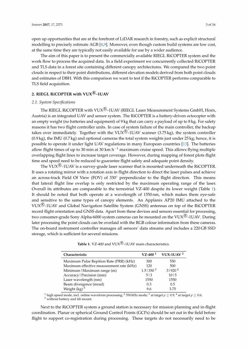
1 high speed mode, incl. online waveform processing; 2 550 kHz mode; 3 at target ρ ≥ 0.9; 4 at target ρ ≥ 0.6;5 without battery and tilt mount.

Next to the RiCOPTER system a ground station is necessary for mission planning and in-flightcoordination. Planar or spherical Ground Control Points (GCPs) should be set out in the field beforeflight to support co-registration during processing. These targets do not necessarily need to be

Sensors 2017, 17, 2371 4 of 16

geolocated in case only internal point cloud registration is to be optimised. However, they should havean adequate size of >0.5 m—depending on flight altitude and scanning speed—to be properly covered.In case sufficient planar surfaces are available in the study area, these can also be used. However, this istypically not the case for forest plots.

2.2. Operations

Necessary legal requirements for professional operations are similar to other UAV operations andmainly involve RiCOPTER registration as an aircraft in the country of operations as well as the trainingand licensing of the pilot. Both processes can partly run in parallel and can take up to several months.Additional to regular licensing the pilot should also become familiar with the flight behaviour of theRiCOPTER, since it is considerably larger than typical mini-UAV. Also the proper operation of the twoindependent flight controllers needs to be trained. Moreover, operation in forest areas usually requirestake off and landing in canopy openings with restricted viewing conditions and options to manoeuvre.Another general preparation includes the identification of a source of base station data that is necessaryfor processing the acquired data. Additionally, legal requirements for the transportation of the batteriesneed to be investigated.

Once these general prerequisites are fulfilled, practical mission planning can begin. This mainlyinvolves getting access permissions to the study site especially from the landowner, arranging transportand notifying other airspace users. Furthermore, the weather forecast should be studied with respectto wind, visibility and humidity to identify the best suitable days for mission execution. As for othermini-UAV the RiCOPTER has a legal limit on wind speed up to which take off is allowed, which is7 m s−1 for the Netherlands. However, wind limits are typically stricter in respect to data quality ascrown movement hampers proper co-registration of point clouds from different flight lines, as is alsothe case for TLS [11].

Initial flight path planning should be performed in preparation of the field work. The target isa certain point density to be achieved by varying flying speed and altitude, and overlap of flight lines.Nonetheless, not anticipated on-site conditions like single emerging trees or lack of emergency landinglocations can demand modification. Transport to the site should take into account the size and weightof the equipment. The RiCOPTER itself is delivered with a transport case of ~120 cm × 80 cm × 55 cm.The ground station has dimensions ~55 cm × 45 cm × 20 cm. At the study site, the area should beinspected to identify take-off and landing as well as emergency landing locations, obstacles close theintended flight path and positions for GCPs. After completion the equipment can be set up and themission executed. After the mission, the raw data is downloaded from the instrument controller.

2.3. Data Processing

RIEGL provides a software suite together with the RiCOPTER system to convert the producedraw data into point clouds. Figure 1 gives an overview of the required steps. While most of the workcan be done in RIEGL’s software for airborne and mobile laser scanning, RiPROCESS, the trajectorypreprocessing has to be accomplished with third party software, e.g., Applanix POSPac MobileMapping Suite. For this purpose additional GNSS base station data has to be acquired. During GNSSpost-processing both data streams from the GNSS antennas and the IMU are taken into account toreconstruct the flight trajectory.

For each flown and logged scan line, the raw scan data has to be subjected to waveform analysisduring which targets are detected within the stored flight line waveforms. Up to four targets can bedetected per pulse. During this process, Multiple Time Around (MTA) range ambiguities have to betaken care of. MTA range ambiguity occurs when pulses are fired before their predecessor pulses canreturn. MTA 1 range, where no ambiguity can occur because a pulse always returns before the next isfired, is at around 100 m range for a Pulse Repition Rate (PRR) of 550 Hz. Thus MTA range ambiguityneeds to be taken care of, but does not result in serious obstacles assuming flying heights below 120 m.The waveform processing detects targets in the scanners own coordinate system. Next, this data is

Sensors 2017, 17, 2371 5 of 16

interpreted with help of the trajectory information and the scanner mounting orientation to producethe first point clouds, one per flight line. The within and across flight line registration is already ofhigh quality as experienced by the authors during several missions and would serve when registrationerror of below 1 m is not an issue.

Visualisation & Flightline

Co-registrationPoint Cloud

Flight Trajectory (Position & Attitude)

GNSS base station data

GNSS Post Processing

Data Coordinate Transformation

Scanner Mounting Orientation

Data in Scanner's Coordinate System

Position (GNSS) & Attitude (INS)

raw dataRaw Scan Data

Waveform analysis &coordinate

transformation

Required process

Optional process

RiPROCESS

GNSS + IMUpost-processor

Figure 1. RiCOPTER processing flowchart (based on [20]).

However, when sub-centimetre accuracy is required, point clouds need to be fine registered.In principal this means to reduce errors in the flight trajectory as the position and orientationerror of the RiCOPTER system (cm scale) is much bigger than the range error of the scanner(mm scale). This process can include two independent steps. One is the within flight line trajectoryoptimisation that is handled by the RiPRECISION package within RiPROCESS. Similar to Multi-StationAdjustment (MSA) for TLS [11] control planes are automatically searched for in the point clouds perflight line. So far this process demands no user interaction. It can be supported by GCPs that have beenindependently located to within millimetres, e.g., with Real Time Kinematic (RTK) GNSS. However,for forest situations this is impractical as GNSS reception is typically too low under closed canopiesto achieve the required accuracy. The other possible optimisation is across flight line optimisationthat can be performed with the Scan Data Adjustment (SDA) package within RiPROCESS. It assumeswithin flight line registration as optimal and only changes the overall position and orientation of flightlines to each other. This can be compared to linking point clouds from single scanning positions in TLS.Here, next to automatically detected planes, also manually digitised control objects, such as planes,spheres and points, can be included to improve the co-registration.

The point cloud processing can be finished off with removal of atmospheric noise, which is visibleas returns close to the flight trajectory with typically low reflectivity, and target type classification.Finished point clouds can be exported from RiPROCESS in common file formats, e.g., ASCII and LAS,to continue analysis in dedicated software packages.

3. Field Experiment

The field experiment took place at the Speulderbos Fiducial Reference site in the Veluweforest area (N52◦15.15′ E5◦42.00′), The Netherlands [21] (www.wur.eu/fbprv). The core site isestablished in a stand composed of European Beech (Fagus sylvatica) with occasional PedunculateOak (Quercus robur) and Sessile Oak (Quercus petraea), and a very open understorey with only fewEuropean Holly (Ilex aquifolium) (Figure 2). The stand was established in 1835 and had a tree density of204 trees/ha. At the time of the experiment the overstorey was in the progress of spring bud break and

Sensors 2017, 17, 2371 6 of 16

leaf unfolding, so that only few trees carried a full leaf canopy. In an earlier inventory campaign theBeech stand has been equipped with a 40 m spaced wooden pole grid that has also been geo-locatedwith RTK GPS and land surveying techniques to an accuracy of better than 0.5 m.

E

E

E

E

E

E

E

E

E

E

E

E

E

E

E

E

E

E

E

EE

E

E

E

E

EE

E

E

E

E

E

E

E

E

E

EE

E

E

E

EE

E

E

E

EE

E

E

E

E

E

E

E E E

p Old Beech and Oak

DouglasFir

Giant Fir

Norway Spruce

YoungBeech

5°41'55"E5°41'50"E5°41'45"E5°41'40"E

52°1

5'6"N

52°1

5'4"N

52°1

5'2"N

52°15'8"N

p Take off positionE TLS scan position

Flight trajectory

¯

100 m

Figure 2. Map of the study site with TLS scan positions (crosses), take off position (red plane), flightlines (blue), target areas, study site location in the Netherlands (red dot in inset), airborne false colourcomposite as background image.

Additional to the Beech stand, sections of Norway Spruce (Picea abies), Giant Fir (Abies grandis),young beech and Douglas Fir (Pseudotsuga menziesii) have been scanned as well with the goal tocapture different forest types in terms of species composition, tree density and canopy architecture.The Norway Spruce and Giant Fir stands were established in 1943 and 1967, respectively, and had nounderstorey species. However, the plots were relatively dense with 676 Trees/ha and 961 Trees/ha,respectively, and many low branches. The young beech stand was established in 1973 and had a densityof 805 Trees/ha. There were no other species present in this stand, but most lower branches werecarrying leaves. The Douglas Fir stand had a very open understorey where only few saplings of up to2 m height could be found. The stand was established in 1959 and has been thinned since then as wasobvious through the present stumps.

The total scanned area covered 100 m × 180 m, roughly 2 ha. In the study area, a forest roadseparates the old beech and oak from the other stands, and a bike path the Giant Fir and NorwaySpruce stands. The UAV take-off area was located in an opening east of the stands that was wideenough to allow Visual Line of Sight (VLOS) operations.

TLS data acquisition was completed in the course of two days that were both marked by verylow wind speeds (<3 m s−1). During the first day the TLS scan position grid was set up. For thatthe wooden poles in the Beech stand were taken as starting positions. With the help of a theodolitethe TLS positions were marked to form a grid of 40 m spacing in the Beech and 20 m spacing in theDouglas Fir stands. Additional positions in the grid centres have been added in the Beech stand.Cylindrical retro-reflective targets were set up for later coarse co-registration of scans [11]. The first15 positions have been scanned during the first day, the remaining 43 during the second day. All scanswere performed with 0.06◦ scan resolution. Due to the VZ-400’s zenithal scan angle range of 30◦ to130◦, an upward and tilted scan had to be performed per scan location to cover the area directly overthe scan position.

To support co-registration of RiCOPTER flight lines 4 large (120 cm × 60 cm) and 8 small(60 cm × 60 cm) ground control panels have been distributed under the trees and next to the take-off

Sensors 2017, 17, 2371 7 of 16

site. The panels consist each of 2 equally sized wooden panes connected via piano hinges. When set upthe panes form a 90◦ angle between them, which makes them look like tents. Cars used for transportwere deliberately parked on the forest road in the scanning area to provide additional control surfacesfor the co-registration. The ground station was erected next to the take off site. The scan lines weredesigned to maximise lateral overlap and efficiently use air time (Figure 2). The RiCOPTER was flownat an altitude of 90 m a.g.l., with a cruise speed of 6 m s−1. The VUX R©-1UAV was operated withthe full FOV of 330◦, a PRR of 550 kHz and scan speed of 58 lines/s, which resulted in an averagerectangular point spacing of ~8 cm and a point density of 140 points/m2 for a single flight line at nadir.Mission time for active scan and non-active connection lines was 9 min to cover a distance of ~2300 m.

4. Methods

In case of TLS, the scans were first coarsely co-registered with automatically extracted tie-pointsbased on the retro-reflective cylinders. These registrations had typical registration errors of <5 cm.Afterwards MSA was applied to refine the registration [11]. This approach automatically searchesfor tie-planes in the scans and iteratively adjusts orientation and position of each scan position tominimise the global fitting error of tie-planes. The resulting standard deviation of the errors over alltie-planes was 0.62 cm. All operations were executed with RIEGL’s RiSCAN PRO R© software package.

For processing of the RiCOPTER data the work-flow as described in Section 2.3 was applied.GNSS data was obtained from 06-GPS (Sliedrecht, The Netherlands) for a virtual base stationin the centre of the study site and the period of the campaign to allow GNSS post-processing.RiPRECSION-UAV was applied to optimise within flight line registration. Automatic across-flight lineregistration with automatic search of tie-planes continuously failed to produce good results, probablydue to missing planar surfaces in the study area. Therefore, the GCP panels were manually digitisedas tie-planes and used for fine registration. Final standard deviation of the fitting errors of 0.97 cm.

The resulting point clouds from TLS and ALS were co-registered via common tie-planes.These were the manually selected GCP panels. Then different raster products were produced at0.5 m resolution with LAStools (https://rapidlasso.com/lastools/): scan density by counting all hitswithin a resolution cell, DTMs by selecting the lowest point in a resolution cell, DSMs with the highest,and Canopy Height Models (CHMs) by calculating the difference between DTMs and DSMs.

The lower stem parts of individual trees were manually extracted from the TLS and ALS pointclouds from the 5 plots (Figure 2). For each tree all points at a height of 120 to 140 cm were selectedto represent DBH. These subsets were manually inspected for the suitability to fit circles. In case ofpresence of branches at the DBH height, the corresponding points were further manually removed.Next, circles were fitted to the horizontal coordinates of these points separately for ALS and TLS.An iterative optimisation procedure was used to minimise the euclidean distance between points andcircles according to Coope [22] as implemented in R’s (http://www.r-project.org/) circular package.Next to the geometries, the points contained information about the return number and scan angleunder which they were recorded. These were analysed to gain more insights which scan conditionscan be beneficial to record stem points.

5. Results

The acquired TLS and ALS point clouds showed a number of differences. Figure 3 shows twosample transects through the Old Beech and Oak area (cf. Figure 2). The ALS point cloud clearly hada lower point density in the stem area, while the branch and leaf area appeared to be of comparabledensity. Nonetheless, single stems as well as larger branches could be made out. It should be notedthat even though the images suggest the trees to have a full canopy, this was not the case during thetime of acquisition. The canopy level rather has a distinctively different apparent reflectance than stemand ground elements, because partial hits are much more likely in the crown area where branches donot completely fill the laser footprint.

Sensors 2017, 17, 2371 8 of 16

(a) ALS

(b) TLS

Figure 3. Old Beech and Oak point clouds samples from same perspective, coloured according toapparent reflectance (blue = low, green = medium, red high).

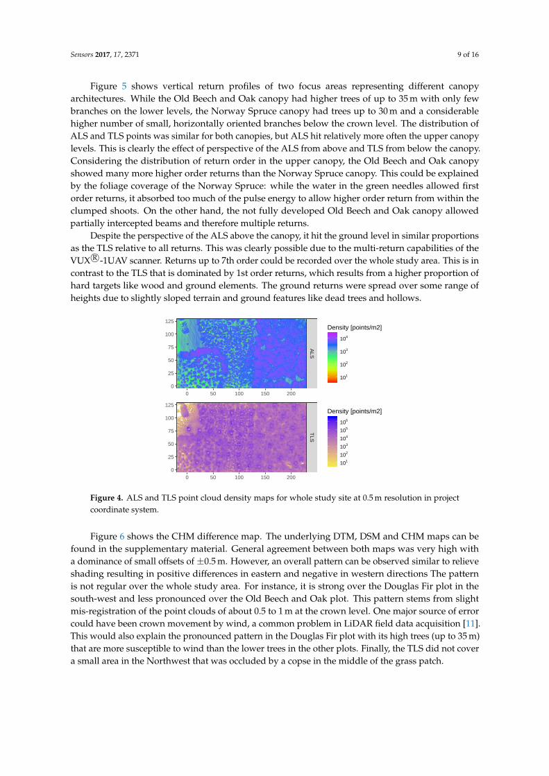
Figure 4 gives an overview of point density over the whole of the study site. While ALS pointdensity was highest in tree crowns, visible as mushroom forms in the Old Beech and Oak area,TLS point density peaked at stem locations, visible as black specks in the TLS map. Furthermore,higher density areas were created by slight horizontal course corrections of the UAV, which are visibleas stripe patterns in the density map, especially in the forest opening in the Northwest. Also morepoints were observed along the centre line of the plot in WE direction due to the higher overlapof flight lines in that area, i.e., northern and southern flight lines contribute to the centre locations.This can be seen when comparing Beech areas close to WE centre line and Beech in upper right ofFigure 4, around [160,60] and [210,110], respectively. In case of TLS fewer points were registered aroundscan positions, which stems from the restriction in zenithal scanning angle of the VZ-400 scanner.Overall, ALS point density was about 2 orders of magnitude lower than TLS for the given scanconfigurations. It was on average 5344 points/m2, 3081 points/m2, 3005 points/m2, 2965 points/m2

and 3004 points/m2 for the Old Beech and Oak, Giant Fir, Norway Spruce, Young Beech, and DouglasFir plots, respectively.

Sensors 2017, 17, 2371 9 of 16

Figure 5 shows vertical return profiles of two focus areas representing different canopyarchitectures. While the Old Beech and Oak canopy had higher trees of up to 35 m with only fewbranches on the lower levels, the Norway Spruce canopy had trees up to 30 m and a considerablehigher number of small, horizontally oriented branches below the crown level. The distribution ofALS and TLS points was similar for both canopies, but ALS hit relatively more often the upper canopylevels. This is clearly the effect of perspective of the ALS from above and TLS from below the canopy.Considering the distribution of return order in the upper canopy, the Old Beech and Oak canopyshowed many more higher order returns than the Norway Spruce canopy. This could be explainedby the foliage coverage of the Norway Spruce: while the water in the green needles allowed firstorder returns, it absorbed too much of the pulse energy to allow higher order return from within theclumped shoots. On the other hand, the not fully developed Old Beech and Oak canopy allowedpartially intercepted beams and therefore multiple returns.

Despite the perspective of the ALS above the canopy, it hit the ground level in similar proportionsas the TLS relative to all returns. This was clearly possible due to the multi-return capabilities of theVUX R©-1UAV scanner. Returns up to 7th order could be recorded over the whole study area. This is incontrast to the TLS that is dominated by 1st order returns, which results from a higher proportion ofhard targets like wood and ground elements. The ground returns were spread over some range ofheights due to slightly sloped terrain and ground features like dead trees and hollows.

ALS

0 50 100 150 2000

25

50

75

100

125

101

102

103

104

Density [points/m2]

TLS

0 50 100 150 2000

25

50

75

100

125

101

102

103

104

105

106

Density [points/m2]

Figure 4. ALS and TLS point cloud density maps for whole study site at 0.5 m resolution in projectcoordinate system.

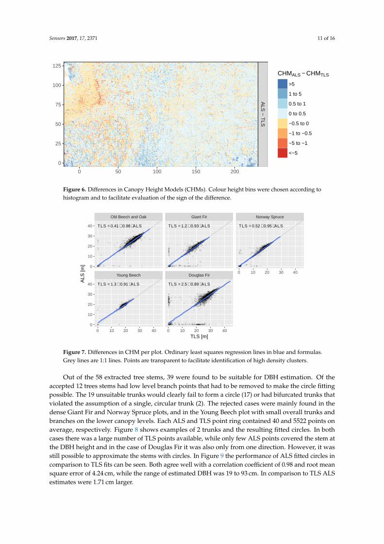
Figure 6 shows the CHM difference map. The underlying DTM, DSM and CHM maps can befound in the supplementary material. General agreement between both maps was very high witha dominance of small offsets of ±0.5 m. However, an overall pattern can be observed similar to relieveshading resulting in positive differences in eastern and negative in western directions The patternis not regular over the whole study area. For instance, it is strong over the Douglas Fir plot in thesouth-west and less pronounced over the Old Beech and Oak plot. This pattern stems from slightmis-registration of the point clouds of about 0.5 to 1 m at the crown level. One major source of errorcould have been crown movement by wind, a common problem in LiDAR field data acquisition [11].This would also explain the pronounced pattern in the Douglas Fir plot with its high trees (up to 35 m)that are more susceptible to wind than the lower trees in the other plots. Finally, the TLS did not covera small area in the Northwest that was occluded by a copse in the middle of the grass patch.

Sensors 2017, 17, 2371 10 of 16

ALS

0e+00 1e+06 2e+06 3e+06 4e+06

10

20

30

40

Kernel point count

Hei

ght [

m]

TLS

0e+00 1e+07 2e+07 3e+07

10

20

30

40

Kernel point count

Return order

1

2

3

4 or more

(a) Old Beech and Oak

ALS

0e+00 1e+05 2e+05 3e+05 4e+05 5e+05

10

20

30

Kernel point count

Hei

ght [

m]

TLS

0e+00 5e+06 1e+07

10

20

30

Kernel point count

Return order

1

2

3

4 or more

(b) Norway Spruce

Figure 5. Vertical return density profiles smoothed with Gaussian kernel of all points in two areas ofinterest (see Figure 2), height reference is lowest point found in sub-area.

The mis-registration can also be found in the scatterplot of height differences in the plots inFigure 7: extreme cases can be found along the x and y axes. They represent cases when either theALS or the TLS hit the crown and the other the ground. Outliers along the x and y axis representmainly the western and eastern crowns sides, respectively. Nonetheless, all scatterplots confirm thehigh agreement of ALS and TLS. However, similar to the vertical profiles (Figure 5) also in the caseof the CHMs ALS tended to detect higher points in the canopy, resulting in overall higher CHM.For instance, the ALS CHM was 6.1 cm and 12.2 cm higher for the Giant Fir and Old Beech and Oakplots, respectively. The difference for all cells over all plots was 11.5 cm.

Sensors 2017, 17, 2371 11 of 16

ALS

− T

LS

0 50 100 150 200

0

25

50

75

100

125

CHMALS − CHMTLS

>5

1 to 5

0.5 to 1

0 to 0.5

−0.5 to 0

−1 to −0.5

−5 to −1

<−5

Figure 6. Differences in Canopy Height Models (CHMs). Colour height bins were chosen according tohistogram and to facilitate evaluation of the sign of the difference.

TLS = 0.41 + 0.98 ⋅ ALS

TLS = 1.3 + 0.91 ⋅ ALS

TLS = 1.2 + 0.93 ⋅ ALS

TLS = 2.5 + 0.89 ⋅ ALS

TLS = 0.52 + 0.95 ⋅ ALS

Young Beech Douglas Fir

Old Beech and Oak Giant Fir Norway Spruce

0 10 20 30 40 0 10 20 30 40

0 10 20 30 400

10

20

30

40

0

10

20

30

40

TLS [m]

ALS

[m]

Figure 7. Differences in CHM per plot. Ordinary least squares regression lines in blue and formulas.Grey lines are 1:1 lines. Points are transparent to facilitate identification of high density clusters.

Out of the 58 extracted tree stems, 39 were found to be suitable for DBH estimation. Of theaccepted 12 trees stems had low level branch points that had to be removed to make the circle fittingpossible. The 19 unsuitable trunks would clearly fail to form a circle (17) or had bifurcated trunks thatviolated the assumption of a single, circular trunk (2). The rejected cases were mainly found in thedense Giant Fir and Norway Spruce plots, and in the Young Beech plot with small overall trunks andbranches on the lower canopy levels. Each ALS and TLS point ring contained 40 and 5522 points onaverage, respectively. Figure 8 shows examples of 2 trunks and the resulting fitted circles. In bothcases there was a large number of TLS points available, while only few ALS points covered the stem atthe DBH height and in the case of Douglas Fir it was also only from one direction. However, it wasstill possible to approximate the stems with circles. In Figure 9 the performance of ALS fitted circles incomparison to TLS fits can be seen. Both agree well with a correlation coefficient of 0.98 and root meansquare error of 4.24 cm, while the range of estimated DBH was 19 to 93 cm. In comparison to TLS ALSestimates were 1.71 cm larger.

Sensors 2017, 17, 2371 12 of 16

Douglas Fir Old Beech and Oak

ALS

TLS

-0.2 0.0 0.2 -0.2 0.0 0.2

-0.2

0.0

0.2

-0.2

0.0

0.2

Figure 8. Samples of fitted circles to estimate DBH in the x-y-plane, x and y axis in cm.

20

40

60

80

20 40 60 80

DBH estimated by TLS [cm]

DB

H e

stim

ated

by

ALS

[cm

]

Tree speciesDouglas Fir

Giant Fir

Norway Spruce

Old Beech and Oak

Young Beech

Figure 9. DBH of TLS compared to ALS. Grey line is 1:1.

Another interesting observation concerned the scan angles and return orders of the ALS pointsthat were available for the DBH estimation. The scan or body across angle is the angle under whicha laser pulse was shot from the scanner. It is 0◦ perpendicular to the rotor arms when mounted,i.e., a scan angle of 0◦ would describe nadir when the RiCOPTER flies perfectly horizontal. Largepositive and negative scan angles result in low incidence angles. Figure 10 shows the distributionof scan angles for the sampled points that were used for the DBH estimation. The distributionswere strongly bimodal for the Old Beech and Oak, Norway Spruce and Douglas Fir plots with peaksbetween −20◦ to −40◦ and 20◦ to 40◦. The distribution of the Young Beech points were dominated bytwo trees that were hit from flight lines with the same orientation, resulting in a peak around −30◦.Even though the RiCOPTER does not always fly perfectly horizontal, because it has to compensate thewind direction, generally scan angles around 30◦ to 40◦ seem to be well suited for detection of trunks.Probably self-occlusion of the observed tree and occlusion by other trees is minimal at these angles.Furthermore, trunk points were constituted of 14.6% 1st, 25.8% 2nd, 29.4% 3rd, and 30.2% 4th or higherreturn order. This underlines that the multi-return capability of the VUX R©-1UAV was beneficial toobserve trunks.

Sensors 2017, 17, 2371 13 of 16

N = 1845

N = 179

N = 128

N = 417

N = 267

Giant Fir Douglas Fir

Old Beech and Oak Young Beech Norway Spruce

−60 −30 0 30 −60 −30 0 30

−60 −30 0 300.000

0.005

0.010

0.015

0.020

0.000

0.005

0.010

0.015

0.020

Scan Angle

Ker

nel D

ensi

ty

Figure 10. ALS scan angles under which the points considered for the DBH estimation were observed.N denotes the number of points for each plot.

6. Discussion

Development of LiDAR technology and algorithms in recent years has shown great potential tosupport forestry practices, in particular geometric characterisation of plots up to unbiased estimationof AGB [4]. In this context TLS yields a data source of unprecedented detail and accuracy. However,TLS acquisition can be labour intense and time consuming especially in challenging environments liketropical forests [11]. New UAV-borne LiDAR technology can possibly accelerate these field campaignsand provide a larger coverage.

In this context, the RIEGL RiCOPTER with VUX R©-1UAV has proven useful to characterise theSpeulderbos forest plot. CHMs were successfully derived and showed good agreement with TLS.Canopy height estimated by the ALS were generally higher. This could be expected by its viewingperspective from above the canopy and the known shortcoming of TLS to not always detect the topof canopy (e.g., [23]). However, the difference of on average 11.5 cm falls within the precision oftraditional field measurements for tree height of 50 cm [24]. Concerning the estimation of individualtree height, Wallace el al. [17] found good agreement with field measurements of 0.35 m (mean absoluteerror) by using point clouds of up to 300 points/m2 density.

Multi-return and side-looking capabilities proved to be important features of the VUX R©-1UAVto scan trunks and estimate DBH for a number of trees under different canopy conditions (Figure 9).While other UAV LiDAR systems are also able to record multiple targets per pulse, not many systemsare able to acquire data under larger scan angles (>30◦ off nadir). Nonetheless, a sufficient number ofpoints could not be collected for all sampled trunks, mainly in the dense, narrow spaced needle-leafplots. Repeated flights over the same plots with varying flight paths could result in better coverage. Theaverage root mean square error of 4.24 cm between TLS and ALS is comparable to reported deviationsof TLS and traditional methods of 0.7 to 7.0 cm (RMSE) [1]. However, the DBH estimation error is stillmuch larger than the precision of traditional methods of ~0.3 cm [24].

The scan angles that proved optimal to scan the trunk samples (Figure 10) have implicationsfor the flight preparation. The targeted plots should be always well covered, possibly with flightlines that overshoot the plot area. For instance if the flight height is at 90 m and the optimal angleis assumed to be 30◦, the flight trajectory should overshoot by ~52 m. However, it is difficult to sayhow general the optimal scan angles found in this study are. In any way, we found that multipleflight lines, made possible through the long air-borne time, were contributing to a better samplingfrom different directions. In this respect more lines at faster speed, should be preferred to fewer atlower speed assuming same airborne time. Maximising line crossings and multiple flights should beconsidered as well. The later will be primarily restricted by the number of battery packs available.

Sensors 2017, 17, 2371 14 of 16

Initial point cloud production of VUX R©-1UAV data solely relies on the on-board IMU and GNSSpost processing. This is possible because of the IMU’s accuracy, which on the other hand results ina large weight for the scanner. This drives the weight of the whole system, since heavier sensors alsorequire larger payload capacity and thus larger UAVs. Together with the system requirement of longendurance this brought the total system weight up to just under the legal limit for mini-UAV (personalcommunication RIEGL, 2016). This design decision makes it unnecessary to employ algorithms thatreconstruct the trajectory in the post-processing as shown in previous studies [16,18]. However,it makes the availability of GNSS base station data a hard requirement that might be difficult to fulfilin remote areas. Also the system weight can be a logistical challenge in such cases.

Even though this study did not aim to conduct full plot inventories, the data shows promisingattributes to extend the analysis in that direction. One important step for this would be to detectsingle trees in all plots. Wallace et al. [25] produced detection rates of up to 98% with point clouds of50 points/m2 density. Therefore, detection should be achievable with the ~3000 points/m2 RiCOPTERpoint clouds. Based on the detected trees, single tree height can be estimated. However, traditionalforest inventory data would be necessary for validation.

Apart from characterising traditional forest metrics, UAV-borne LiDAR could also be utilisedas a flexible, higher resolution alternative to manned airborne LiDAR, especially to study foliage.In that case several published algorithms could be employed [26–29] and tested if they are applicableon higher density point clouds. Moreover, reliable and mobile systems like the RiCOPTER are suitablefor multi-temporal studies [15].

7. Conclusions

This study presented first results and experiences with the RIEGL RiCOPTER with VUX R©-1UAVALS with its components and processing work flow, and its performance in estimating CHM andDBH compared to TLS. As first steps we compared the RiCOPTER with the well tested RIEGL VZ-400TLS by deriving CHM and estimating DBH. CHMs showed only small differences that could beexplained by the perspective of the RiCOPTER above the canopy, resulting in different vertical detectionprofiles that facilitate the discovery of highest points in the canopy, which is not always possiblewith TLS. Additionally, the multi-return and side-looking capabilities of the VUX R©-1UAV scannerproved beneficial to detect trunk elements. This feature will be valuable when more sophisticated3D modelling is to be applied. However, not all sampled tree trunks were sufficiently covered withpoints, so that more flights or different flight patterns are necessary to achieve better coverage. Overall,the RiCOPTER could produce comparable results to the VZ-400. Further experiments should bedirected to test explicit quantitative structural modelling to derive AGB from the RiCOPTER pointclouds as well as co-registration strategies of multiple flights and with TLS systems.

Supplementary Materials: The following are available online at http://www.mdpi.com/1424-8220/17/10/2371/s1,Figure S1: Digital Elevation Models at 0.5 m resolution in project coordinate system, blank cells did not containpoints; Figure S2: Digital Surface Models at 0.5 m resolution in project coordinate system, blank cells did notcontain points; Figure S3: Canopy Height Models at 0.5 m resolution in project coordinate system, blank cells didnot contain points.

Acknowledgments: This work was carried out as part of the IDEAS+ contract funded by ESA-ESRIN. A.L. issupported by CIFOR’s Global Comparative Study on REDD+, with financial support from the InternationalClimate Initiative (IKI) of the German Federal Ministry for the Environment and the donors to the CGIARFund. The access to the RiCOPTER has been made possible by Shared Research Facilities of WageningenUniversity & Research. The authors thank the Dutch Forestry Service (Staatsbosbeheer) for granting access tothe site and 06-GPS for supplying the GNSS base station data. Further thanks go to Marcello Novani for helpduring the fieldwork and Jan den Ouden to identify the tree species. We thank two anonymous reviewers fortheir helpful comments to improve the quality of this manuscript.

Author Contributions: B.B. and H.M.B. conceived and designed the experiment; B.B., A.L. and H.M.B. conductedthe field experiment; B.B. and A.L. analysed the data; H.M.B. and L.K. scientifically supported and reviewed thepaper; L.K. arranged licensing of the UAV; B.B. wrote the paper.

Conflicts of Interest: The authors declare no conflict of interest.

Sensors 2017, 17, 2371 15 of 16

References

1. Liang, X.; Kankare, V.; Hyyppä, J.; Wang, Y.; Kukko, A.; Haggrén, H.; Yu, X.; Kaartinen, H.; Jaakkola, A.;Guan, F.; et al. Terrestrial laser scanning in forest inventories. ISPRS J. Photogramm. Remote Sens. 2016,115, 63–77.

2. Newnham, G.J.; Armston, J.D.; Calders, K.; Disney, M.I.; Lovell, J.L.; Schaaf, C.B.; Strahler, A.H.; Danson, F.M.Terrestrial Laser Scanning for Plot-Scale Forest Measurement. Curr. For. Rep. 2015, 1, 239–251.

3. Gonzalez de Tanago, J.; Lau, A.; Bartholomeus, H.; Herold, M.; Avitabile, V.; Raumonen, P.; Martius, C.;Goodman, R.; Manuri, S.; Disney, M.; et al. Estimation of above-ground biomass of large tropical trees withTerrestrial LiDAR. Methods Ecol. Evol. 2017, doi:10.1111/2041-210X.12904.

4. Calders, K.; Newnham, G.; Burt, A.; Murphy, S.; Raumonen, P.; Herold, M.; Culvenor, D.; Avitabile, V.;Disney, M.; Armston, J.; et al. Nondestructive estimates of above-ground biomass using terrestrial laserscanning. Methods Ecol. Evol. 2015, 6, 198–208.

5. Le Toan, T.; Quegan, S.; Davidson, M.W.J.; Balzter, H.; Paillou, P.; Papathanassiou, K.; Plummer, S.; Rocca, F.;Saatchi, S.; Shugart, H.; et al. The BIOMASS mission: Mapping global forest biomass to better understandthe terrestrial carbon cycle. Remote Sens. Environ. 2011, 115, 2850–2860.

6. Eitel, J.U.; Höfle, B.; Vierling, L.A.; Abellán, A.; Asner, G.P.; Deems, J.S.; Glennie, C.L.; Joerg, P.C.;LeWinter, A.L.; Magney, T.S.; et al. Beyond 3-D: The new spectrum of LiDAR applications for earthand ecological sciences. Remote Sens. Environ. 2016, 186, 372–392.

7. Wallis, C.I.; Paulsch, D.; Zeilinger, J.; Silva, B.; Curatola Fernández, G.F.; Brandl, R.; Farwig, N.; Bendix, J.Contrasting performance of LiDAR and optical texture models in predicting avian diversity in a tropicalmountain forest. Remote Sens. Environ. 2016, 174, 223–232.

8. Morsdorf, F.; Nichol, C.; Malthus, T.; Woodhouse, I.H. Assessing forest structural and physiological informationcontent of multi-spectral LiDAR waveforms by radiative transfer modelling. Remote Sens. Environ. 2009,113, 2152–2163.

9. Raumonen, P.; Kaasalainen, M.; Åkerblom, M.; Kaasalainen, S.; Kaartinen, H.; Vastaranta, M.; Holopainen, M.;Disney, M.; Lewis, P. Fast Automatic Precision Tree Models from Terrestrial Laser Scanner Data. Remote Sens.2013, 5, 491–520.

10. Hackenberg, J.; Morhart, C.; Sheppard, J.; Spiecker, H.; Disney, M. Highly accurate tree models derived fromterrestrial laser scan data: A method description. Forests 2014, 5, 1069–1105.

11. Wilkes, P.; Lau, A.; Disney, M.I.; Calders, K.; Burt, A.; Gonzalez de Tanago, J.; Bartholomeus, H.; Brede, B.; Herold,M. Data Acquisition Considerations for Terrestrial Laser Scanning of Forest Plots. Remote Sens. Environ. 2017,196, 140–153.

12. Colomina, I.; Molina, P. Unmanned aerial systems for photogrammetry and remote sensing: A review.ISPRS J. Photogramm. Remote Sens. 2014, 92, 79–97.

13. Torresan, C.; Berton, A.; Carotenuto, F.; Di Gennaro, S.F.; Gioli, B.; Matese, A.; Miglietta, F.; Vagnoli, C.;Zaldei, A.; Wallace, L. Forestry applications of UAVs in Europe: A review. Int. J. Remote Sens. 2016,38, 2427–2447.

14. Suomalainen, J.; Anders, N.; Iqbal, S.; Roerink, G.; Franke, J.; Wenting, P.; Hünniger, D.; Bartholomeus, H.;Becker, R.; Kooistra, L. A Lightweight Hyperspectral Mapping System and Photogrammetric ProcessingChain for Unmanned Aerial Vehicles. Remote Sens. 2014, 6, 11013–11030.

15. Jaakkola, A.; Hyyppä, J.; Kukko, A.; Yu, X.; Kaartinen, H.; Lehtomäki, M.; Lin, Y. A low-cost multi-sensoralmobile mapping system and its feasibility for tree measurements. ISPRS J. Photogramm. Remote Sens. 2010,65, 514–522.

16. Wallace, L.; Lucieer, A.; Watson, C.; Turner, D. Development of a UAV-LiDAR system with application toforest inventory. Remote Sens. 2012, 4, 1519–1543.

17. Wallace, L.; Musk, R.; Lucieer, A. An assessment of the repeatability of automatic forest inventory metricsderived from UAV-borne laser scanning data. IEEE Trans. Geosci. Remote Sens. 2014, 52, 7160–7169.

18. Chisholm, R.A.; Cui, J.; Lum, S.K.Y.; Chen, B.M. UAV LiDAR for below-canopy forest surveys. J. UnmannedVeh. Syst. 2013, 01, 61–68.

19. Wei, L.; Yang, B.; Jiang, J.; Cao, G.; Wu, M. Vegetation filtering algorithm for UAV-borne LiDAR pointclouds: A case study in the middle-lower Yangtze River riparian zone. Int. J. Remote Sens. 2017, 38, 1–12.

Sensors 2017, 17, 2371 16 of 16

20. RIEGL LMS RiProcess for RIEGL Scan Data. Available online: http://www.riegl.com/uploads/tx_pxpriegldownloads/11_Datasheet_RiProcess_2016-09-16_03.pdf (accessed on 13 September 2017).

21. Brede, B.; Bartholomeus, H.; Suomalainen, J.; Clevers, J.; Verbesselt, J.; Herold, M.; Culvenor, D.; Gascon, F.The Speulderbos Fiducial Reference Site for Continuous Monitoring of Forest Biophysical Variables.In Proceedings of the Living Planet Symposium 2016, Prague, Czech Republic, 9–13 May 2016; p. 5.

22. Coope, I.D. Circle fitting by linear and nonlinear least squares. J. Optim. Theory Appl. 1993, 76, 381–388.23. Hilker, T.; van Leeuwen, M.; Coops, N.C.; Wulder, M.A.; Newnham, G.J.; Jupp, D.L.B.; Culvenor, D.S.

Comparing canopy metrics derived from terrestrial and airborne laser scanning in a Douglas-fir dominatedforest stand. Trees 2010, 24, 819–832.

24. Luoma, V.; Saarinen, N.; Wulder, M.A.; White, J.C.; Vastaranta, M.; Holopainen, M.; Hyyppä, J.Assessing precision in conventional field measurements of individual tree attributes. Forests 2017, 8, 38.

25. Wallace, L.; Lucieer, A.; Watson, C.S. Evaluating tree detection and segmentation routines on very highresolution UAV LiDAR data. IEEE Trans. Geosci. Remote Sens. 2014, 52, 7619–7628.

26. Tang, H.; Brolly, M.; Zhao, F.; Strahler, A.H.; Schaaf, C.L.; Ganguly, S.; Zhang, G.; Dubayah, R. Deriving andvalidating Leaf Area Index (LAI) at multiple spatial scales through LiDAR remote sensing: A case study inSierra National Forest, CA. Remote Sens. Environ. 2014, 143, 131–141.

27. García, M.; Gajardo, J.; Riaño, D.; Zhao, K.; Martín, P.; Ustin, S. Canopy clumping appraisal using terrestrialand airborne laser scanning. Remote Sens. Environ. 2015, 161, 78–88.

28. Morsdorf, F.; Kötz, B.; Meier, E.; Itten, K.I.; Allgöwer, B. Estimation of LAI and fractional cover from smallfootprint airborne laser scanning data based on gap fraction. Remote Sens. Environ. 2006, 104, 50–61.

29. Detto, M.; Asner, G.P.; Muller-Landau, H.C.; Sonnentag, O. Spatial variability in tropical forest leaf areadensity from Multireturn LiDAR and modelling. J. Geophys. Res. Biogeosci. 2015, 120, 1–16.

c© 2017 by the authors. Licensee MDPI, Basel, Switzerland. This article is an open accessarticle distributed under the terms and conditions of the Creative Commons Attribution(CC BY) license (http://creativecommons.org/licenses/by/4.0/).