Fernanda Cristina deMoraes Takafuji

e-mail: fernanda.takafuji@gmail.com

Clovis de Arruda Martinse-mail: cmartins@usp.br

Department of Mechanical Engineering,

Av. Prof. Mello Moraes, 2231,

University of Sao Paulo,

05508-970 Sao Paulo, SP, Brazil

Comparison Between FrequencyDomain and Time Domain RiserAnalysisIn the optimization or parametric analyses of risers, several configurations must be ana-lyzed. It is laborious to perform time domain solutions for the dynamic analysis, sincethey are time-consuming tasks. So, frequency domain solutions appear to be a possiblealternative, mainly in the early stages of a riser design. However, frequency domain anal-ysis is linear and requires that nonlinear effects are treated. The aim of this paper is topresent a possible way to treat some of these nonlinearities, using an iterative process to-gether with an analytical correction, and compare the results of a frequency domainanalysis with the those of a full nonlinear analysis. [DOI: 10.1115/1.4006149]

1 Introduction

Risers are elements that connect the oil well, at the sea bottom,to the floating production unit. They are susceptible to loadscaused by ocean currents and waves. The global analysis aims tostudy the riser behavior due to those environmental loads. This isan essentially nonlinear problem, since it includes large displace-ments, unilateral contact, and nonlinear viscous damping loads.

The structural analysis can be divided into two stages: staticanalysis and dynamic analysis. For riser analyses, the static oneconsiders the loads that are time independent: weight, buoyancy,and current loads. Although the current’s velocity profile varieswith time, its scale of variation is substantially greater than thefirst natural period of the riser and, therefore, it can be consideredconstant. The dynamic analysis includes wave loads and themovement induced at the riser’s top by the floating unit.

To take into account all the nonlinearities of the problem, thedynamic analysis must be performed in the time domain. It meansthat the response is calculated for every time step and the simula-tion time depends on the time that the transient response takes todie away. To achieve convergence, the time step must be smalland, for that reason, a time domain analysis could take a long time.

To choose the most suitable configuration for a given applica-tion, in the first stages of a riser design, several configurationsmust be simulated through a parametric analysis or optimizationmethods. Frequency domain solutions appear as an alternative toconsiderably reduce the time spent in dynamic analyses however,to implement them, all of the nonlinearities have to be treated orremoved somehow.

The purpose of this work is to present a possible way to addressthe nonlinearities inherent in the analysis of risers, concludingthat frequency domain analysis can give similar results to the onesobtained with a time domain analysis for harmonic seas. Toachieve this purpose some results of a case study, obtained withboth methods, were compared. Two different configurations wereconsidered: free-hanging and lazy-wave.

The analyses in the time domain were performed using Orca-flexTM version 9.4a; see Ref. [1] for further information. The fre-quency domain analyses were performed using in-house softwarewhose model and linearization process are presented in this paper.

Despite its importance, vortex-induced vibration (VIV) isbeyond the scope of this work and will not be considered inthe models presented here. Methods of transformation of real

(random) sea states into harmonic sea states will also not be dis-cussed in this paper.

2 Modeling

2.1 Static. The aim of the static analysis is to find the staticbalance configuration and the forces and moments acting on theriser when it is subjected to time-invariant loads.

Although this work focuses on the dynamic analysis, the staticconfiguration is important since it can be used as the initial config-uration of the dynamic analysis and in the frequency domain thedynamic response is considered to be a perturbation of this config-uration. There are many different ways to perform the static analy-sis. Patel and Seyed [2] provide a wide-ranging bibliography onthis topic. A good approximation of the static solution can beobtained with the catenary equations, which consider the weightand buoyancy, but no bending stiffness. Other approaches includethe bending stiffness and other effects. Since the focus of thiswork is on the dynamic solution, any approach could be used toobtain the static configuration. The solution that is brieflydescribed next is the one used here.

The static model is based on the model presented in Santos [3].This reference is in Portuguese, but Silveira and Martins [4] presenta similar numerical solution for two-dimensional problems and Sil-veira and Martins [5] show a solution for three-dimensional ones.

The static loads considered in that work are: weight, buoyancy,and drag caused by the sea water current, which is considered con-stant in time, since the time scale of the variation of the mean ve-locity of the current is substantially greater than the first naturalperiod of the riser. The riser is initially modeled without the bend-ing stiffness, which causes a discontinuity of the curvature in thetouchdown point (TDP) and top regions. Since this discontinuityis not real, it is removed afterwards through a boundary layer tech-nique, as presented in Aranha et al. [6]. The seabed is consideredplain, horizontal, and rigid.

Risers with different segments can be analyzed considering thatthe mechanical properties are constant within each segment. Theaxial stiffness is included and it is assumed that the riser’s mate-rial is always in the elastic regime.

The differential equations that describe the static behavior ofthe riser are then obtained. The boundary conditions are: the posi-tion where the riser is connected on the float unit is known, theposition of the other extreme coincides with the origin of the coor-dinate system, and the vertical coordinate z ¼ 0 at the TDP, how-ever, the curvilinear coordinate s at the TDP is unknown. Thestatic analysis consists of obtaining the solution of the differentialequations considering the boundary conditions. However, since

Contributed by the Ocean Offshore Mechanics and Arctic Engineering Division ofASME for publication in the JOURNAL OF OFFSHORE MECHANICS AND ARCTIC

ENGINEERING. Manuscript received August 16, 2010; final manuscript received October10, 2011; published online May 30, 2012. Assoc. Editor: Daniel T. Valentine.

Journal of Offshore Mechanics and Arctic Engineering NOVEMBER 2012, Vol. 134 / 041301-1Copyright VC 2012 by ASME

Downloaded 06 Jun 2012 to 143.107.98.250. Redistribution subject to ASME license or copyright; see http://www.asme.org/terms/Terms_Use.cfm

the boundary conditions are known for more than one position,the integration could be started at the anchor or at the top using ashooting method, as described by Keller [7].

The numerical integration of the differential equations is performedthrough a 3-4 Runge-Kutta method, with an adaptive step. Thismethod was used in Martins [8] and the step is inversely proportionalto the curvature. Further information on the model, ordinary differen-tial equations, and numerical integration can be found in [3–5].

2.2 Dynamic. There are different ways to dynamically ana-lyze the riser. The model used in this work is briefly describednext. However, the linearization methods presented in the nextsection could be used with different models as well.

The dynamic loads considered in this work are: drag caused bywaves and sea current and the prescribed movement of the float-ing unit. Part of the drag force caused by the current has alreadybeen considered in the static analysis. However, the drag forcecaused by the waves, along with the combined effect of the waveand the current, is considered in the dynamic analysis.

Besides the hypotheses considered in the static analysis, it isalso assumed here that the dynamic loads are harmonic. Thus, theamplitude and period of the waves are known and the float unit’smotion is prescribed through amplitudes and phases relative to thewave. The period of the prescribed motion is considered to be thesame as the wave’s. The static configuration is not updated duringthe dynamic simulation and the dynamic response is assumed tobe a perturbation of the static configuration.

The solution is numerically obtained through the finite elementmethod. The riser is represented by Euler-Bernoulli beams and theequation that governs its dynamics is

M€qðtÞ þ Cð _qðtÞÞ _qðtÞ þ KðqðtÞÞqðtÞ ¼ pð _qðtÞÞ (1)

where M is the mass matrix including the effect of the additionalmass, Cð _qðtÞÞ is the damping matrix, which depends on the riservelocity, K is the elastic and geometric stiffness matrix andpð _qðtÞÞ is the external load. Here, €q, _q, and q are the acceleration,velocity, and displacement vectors of the structure, respectively.All of the global matrices depend on the position of the riser at ev-ery time step.

We consider a harmonic surface wave, traveling in deep water.One of the extremities of the riser is connected to the floating unit,which moves as the waves go by. The motion is transmitted to thetop, making the whole riser move.

Different from the time domain analysis, where the criteriaused to obtain the wave velocity above the mean wave level is toconsider that it is the same velocity of the particles at the meanwave level, in the frequency domain, it is assumed that the par-ticle’s velocity above the mean wave level is zero.

3 Linearization

3.1 Linearization of Rotation and Stiffness. One of the non-linear effects inherent in the dynamic analysis of risers concerns thegeometrical stiffness matrix. It depends on the tension of the ele-ments, which changes dynamically. In addition, so does the positionof the riser, which should be known at each time step in order torotate all of the elements’ matrices to form the global ones.

To treat both nonlinearities, we consider that the dynamicresponse is a perturbation of the static configuration, thus, it isassumed that the matrices do not change during the analysis.

3.2 Linearization of Damping. In this section, a lineariza-tion method for the viscous damping will be presented. The vis-cous part of Morison’s formula, presented in Morison et al. [9], isa quadratic equation in the relative velocity, as is shown next

~fD;t ¼ �1

2qaDCD;t ~vm;t �~vc;t

�� �� ~vm;t �~vc;t

� �(2)

where~vm is the relative velocity between the riser’s velocity _q andthe wave’s velocity ~vw, ~vc is the current velocity, D is the riser’sdiameter, CD is the drag coefficient, qa is the fluid density, and theindex t is related to the transversal direction.

There are many ways to treat this nonlinear effect for the fre-quency domain analysis. The first works concerning the lineariza-tion of drag forces were performed in two dimensions. In thiscase, the problem can be treated as a scalar, as observed by Dantaset al. [10]. One example is the work of Gudmestad and Connor[11], where the approximation vw � _qj j � vw � _qð Þ � vwj j � vw � _qð Þis considered and the linear form is obtained from a least squaresapproximation.

Langley [12] presents a three-dimensional linearization throughthe minimization of the mean squared error and Leira [13] com-pares different methods of linearization. Chen and Lin [14] pro-pose using a Fourier expansion up to any nth order.

Liu and Bergdahl [15] propose a linearization method wherethe work done by the motion of the cable in the time domain isequated to the work in the frequency domain. This is similar tothe method presented in Martins [16] for two dimensionalproblems.

In the method presented in Martins [16], only one linearizationcoefficient is used for the whole riser. Takafuji and Martins [17]extended that work, proposing that one coefficient is used for eachelement. That method was extended in Takafuji [18] for three-dimensional cases using one coefficient per element for the trans-versal force. According to Teng and Li [19], if only one coeffi-cient is used, the linearized drag force can be too large in onedirection and too small in the other one. Therefore, they suggestedthe use of two coefficients per element and that will be used inthis work as well.

The suggested methodology is based on maintaining the dissi-pated energy in one cycle. The coefficients depend on the relativevelocity between the fluid and the riser, which is unknown at thebeginning of the analysis. For that reason, the coefficients are iter-atively obtained. The iterative process is necessary to take intoaccount, as closely as possible, the nonlinearity caused by Mori-son’s formula.

In the three-dimensional problem, the riser does not have onetransversal direction, as in the two-dimensional one. It has a trans-versal plane instead, which changes along the length. For this rea-son, the linearization force is placed in a fixed base ~i;~j; ~k

� �, with

the origin on the anchor.Next, we describe how the linear expression for the transversal

direction is obtained. The linear expression for the axial directionis obtained in an analogous way.

The viscous part of Morison’s formula for the dynamic analysisin the transversal direction is given by

~f D;t ¼�1

2qaDCD;t ~vm;t �~vc;t

�� �� ~vm;t �~vc;t

� �� 1

2qaDCD;t ~vc;t

�� �� ~vc;t

� � (3)

The first part of Eq. (3) corresponds to the total force and the sec-ond part corresponds to the force caused by the current that has al-ready been considered in the static analysis.

To solve the problem in the frequency domain, it is necessarythat the dynamic damping force is approximated to a harmonicforce. Considering that~vm;t is harmonic, one can write a linearizeddamping force as

~~f D;t ¼ �1

2qaDCD;t:

Kt1 0

0 Kt2

� �:~vm;t1

~vm;t2

� �(4)

where Kt1 is the linearization coefficient in transversal direction~t1and Kt2 is the linearization coefficient in the other transversal

041301-2 / Vol. 134, NOVEMBER 2012 Transactions of the ASME

Downloaded 06 Jun 2012 to 143.107.98.250. Redistribution subject to ASME license or copyright; see http://www.asme.org/terms/Terms_Use.cfm

direction~t2. Here,~t1 and~t2 are orthogonal vectors that define thetransversal plane. In addition, the indexes t1 and t2 are related tothe directions~t1 and~t2.

However, the coefficients Kt1 and Kt2 are not known at the be-ginning of the analysis and their values have to be estimated.Since the main purpose of the damping is energy dissipation, thechosen criteria to find an equivalent linear expression is to keepthe dissipated energy in one cycle with period T. It means toimpose that

ð T

0

~f D;ti � _~qtdt ¼ð T

0

~~f D;ti � _~qtdt (5)

where the index i can be direction 1 or 2.Substituting Eqs. (3) and (4) into Eq. (5) leads to

ð T

0

~vm;t �~vc;t

�� �� ~vm;ti �~vc;ti

� �þ ~vc;t

�� ��~vc;ti

� �_~qt � dt

¼ Kti

ðT

0

~vm;ti � _~qt � dt (6)

The relative velocity between the riser and the wave can be writ-ten in the base ~i;~j; ~k

� �in the harmonic way

~vm;t ¼Axx � sin xtþ /xð Þ~iþ Ayx � sin xtþ /y

� �~j

þ Azx � sin xtþ /zð Þ~k (7)

where x ¼ 2p=T. The velocity of the riser in the harmonic waycan be written as

_~qt ¼ Cxx � sin xtþ uxð Þ~iþ Cyx � sin xtþ uy

� �~j

þ Czx � sin xtþ uzð Þ~k (8)

Additionally, the current velocity can be written as

~vc;t ¼ Vt;x~iþ Vt;y

~jþ Vt;z~k (9)

Inserting Eqs. (7), (8), and (9) into Eq. (6), isolating Kti, and con-sidering that

ðT

0

sin xtþ kð Þdt ¼ 0

and

ðT

0

sin xtþ k1ð Þ � sin xtþ k2ð Þdt ¼ px

cos k1 � k2ð Þ

One can obtain

Kti ¼I1

I2

(10)

where

I1 ¼ðT

0

Axx sin xtþ /xð Þ � Vt;x

� �2�

þ Ayx sin xtþ /y

� �� Vt;y

� �2

þ Azx sin xtþ /zð Þ � Vt;z

� �2�1=2

Axix sin xtþ /xið Þ � Vt;xi

� �Cxx sin xtþ uxð Þ

þ Ayix sin xtþ /yi

� �� Vt;yi

� �Cyx sin xtþ uy

� �þ Azix sin xtþ /zið Þ � Vt;zi

� �Czx sin xtþ uzð Þ

� dt

and

I2 ¼ px AxiCx cos /xi � uxð Þ þ AyiCy cos /yi � uy

� ��þAziCz cos /zi � uzð ÞÞ

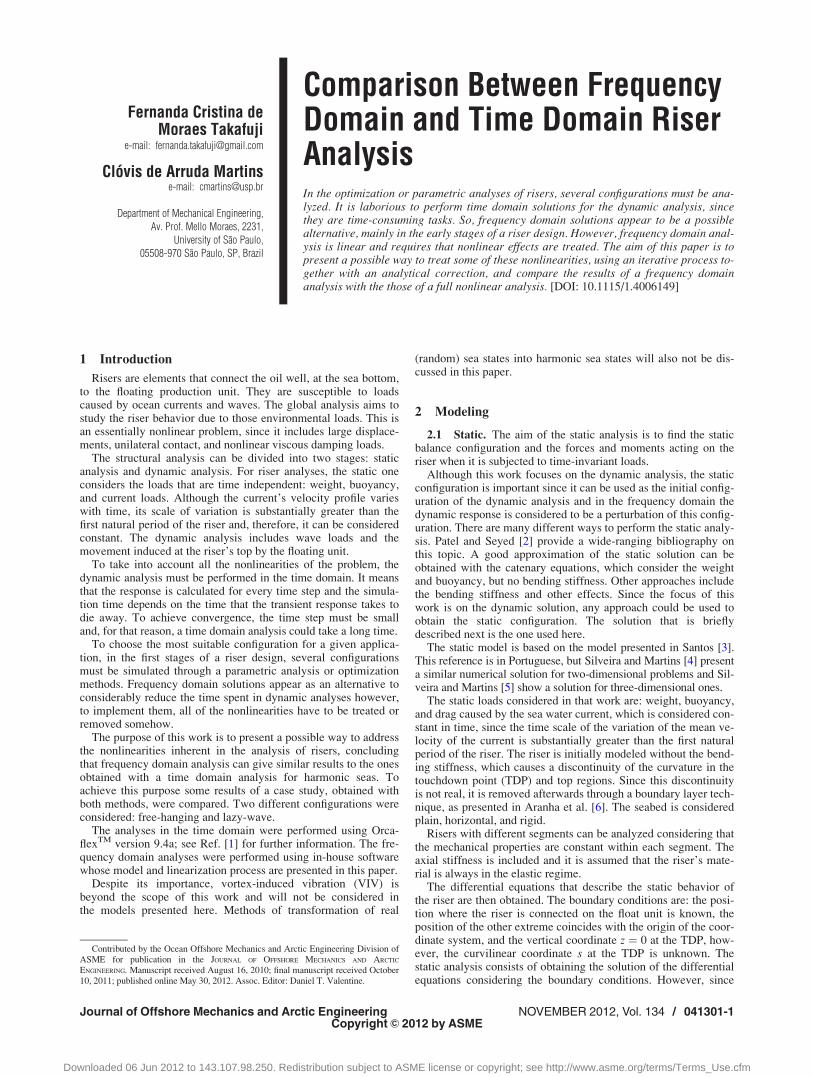
3.3 Linearization of the Riser-Seabed Contact. Anothernonlinearity that should be treated for the frequency domain anal-ysis is the riser-soil contact. During the dynamic analysis, theTDP changes as the floating unit moves, as shown in Fig. 1.

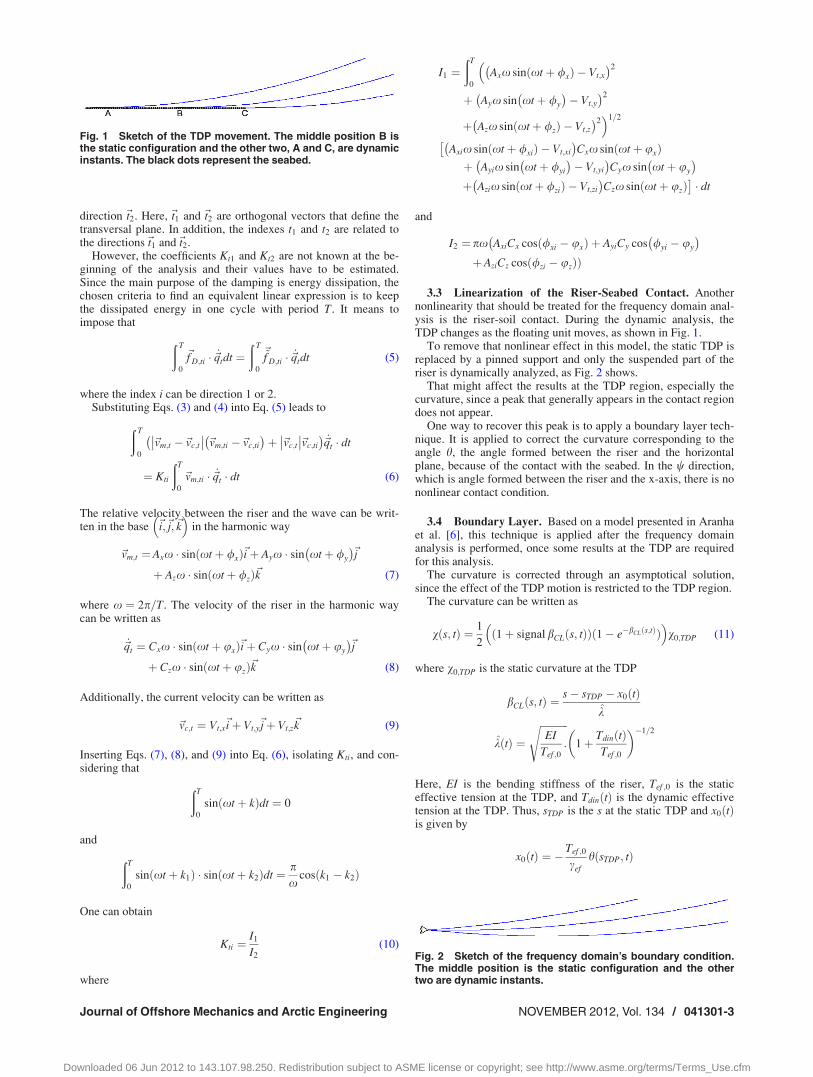
To remove that nonlinear effect in this model, the static TDP isreplaced by a pinned support and only the suspended part of theriser is dynamically analyzed, as Fig. 2 shows.

That might affect the results at the TDP region, especially thecurvature, since a peak that generally appears in the contact regiondoes not appear.

One way to recover this peak is to apply a boundary layer tech-nique. It is applied to correct the curvature corresponding to theangle h, the angle formed between the riser and the horizontalplane, because of the contact with the seabed. In the w direction,which is angle formed between the riser and the x-axis, there is nononlinear contact condition.

3.4 Boundary Layer. Based on a model presented in Aranhaet al. [6], this technique is applied after the frequency domainanalysis is performed, once some results at the TDP are requiredfor this analysis.

The curvature is corrected through an asymptotical solution,since the effect of the TDP motion is restricted to the TDP region.

The curvature can be written as

vðs; tÞ ¼ 1

2ð1þ signal bCLðs; tÞÞð1� e�bCLðs;tÞÞ� �

v0;TDP (11)

where v0;TDP is the static curvature at the TDP

bCLðs; tÞ ¼s� sTDP � x0ðtÞ

k

kðtÞ ¼ffiffiffiffiffiffiffiffiffiffiffiEI

Tef ;0:

s1þ TdinðtÞ

Tef ;0

� �1=2

Here, EI is the bending stiffness of the riser, Tef ;0 is the staticeffective tension at the TDP, and TdinðtÞ is the dynamic effectivetension at the TDP. Thus, sTDP is the s at the static TDP and x0ðtÞis given by

x0ðtÞ ¼ �Tef ;0

cef

hðsTDP; tÞ

Fig. 1 Sketch of the TDP movement. The middle position B isthe static configuration and the other two, A and C, are dynamicinstants. The black dots represent the seabed.

Fig. 2 Sketch of the frequency domain’s boundary condition.The middle position is the static configuration and the othertwo are dynamic instants.

Journal of Offshore Mechanics and Arctic Engineering NOVEMBER 2012, Vol. 134 / 041301-3

Downloaded 06 Jun 2012 to 143.107.98.250. Redistribution subject to ASME license or copyright; see http://www.asme.org/terms/Terms_Use.cfm

where hðsTDP; tÞ is obtained through the frequency domain analy-sis with the articulated joint at the TDP and cef is the effectiveweight per unit of the length of the riser.

According to this model, there is a peak of the dynamic ampli-tude of the curvature that occurs in s ¼ sTDP þ x0ðtÞ, the farthestsection from the TDP for which the condition bCLðs; tÞ � 0 occurs.

4 Frequency Domain Solution

Considering that all the nonlinearities have been removed andthat the excitation is harmonic, the equation of motion can bewritten as

M€qðtÞ þ C _qðtÞ þ KqðtÞ ¼ p0eixt (12)

and the displacement can be written as

qðtÞ ¼ q0eixt (13)

Thus, the first and the second derivatives of the displacements are

_qðtÞ ¼ ix q0eixt (14)

€qðtÞ ¼ �x2q0eixt (15)

Therefore, Eq. (13) can be rewritten as

ð�x2M þ ixCþ KÞq0eixt ¼ p0eixt (16)

Defining the dynamic matrix D as

D ¼ �x2M þ ixCþ K (17)

it can be replaced in Eq. (17) to obtain

D � q0 ¼ p0 (18)

Equation (18) shows that to solve the problem in the frequencydomain corresponds to solving a system of linear algebraic equa-tions. Nevertheless, this system has to be solved several times,because of the linearization of the damping. Since the riser veloc-ity is not known at the beginning of the analysis, the linearization

factor is iteratively obtained, which means that the matrix Cchanges in each iteration and, consequently, the matrix D changesas well. The stop criteria, used in this work, considers that the rel-ative difference of the amplitude of each node’s movement issmaller than a given precision.

5 Case Study

The case study consists of the same steel riser in two differentconfigurations. The first configuration is a steel catenary riser with16 in. of external diameter and 1 in. of thickness. The propertiescan be found in Table 1.

The second configuration is a steel lazy-wave with the proper-ties presented in Table 2.

The environmental and geometrical data for this analysis can befound in Table 3.

Table 4 shows the wave and motion that is prescribed in thefloating unit. It is considered that the riser is installed in a floatingproduction storage and offloading (FPSO) and subjected to atypical centenary wave in the Campos Basin, presented in DNV-OS-E301 [20].

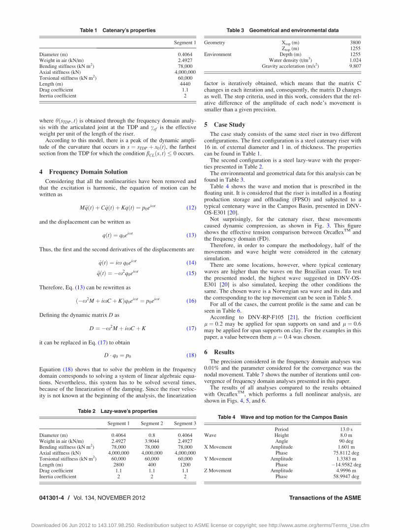
Not surprisingly, for the catenary riser, these movementscaused dynamic compression, as shown in Fig. 3. This figureshows the effective tension comparison between OrcaflexTM andthe frequency domain (FD).

Therefore, in order to compare the methodology, half of themovements and wave height were considered in the catenarysimulation.

There are some locations, however, where typical centenarywaves are higher than the waves on the Brazilian coast. To testthe presented model, the highest wave suggested in DNV-OS-E301 [20] is also simulated, keeping the other conditions thesame. The chosen wave is a Norwegian sea wave and its data andthe corresponding to the top movement can be seen in Table 5.

For all of the cases, the current profile is the same and can beseen in Table 6.

According to DNV-RP-F105 [21], the friction coefficientl ¼ 0:2 may be applied for span supports on sand and l ¼ 0:6may be applied for span supports on clay. For the examples in thispaper, a value between them l ¼ 0:4 was chosen.

6 Results

The precision considered in the frequency domain analyses was0.01% and the parameter considered for the convergence was thenodal movement. Table 7 shows the number of iterations until con-vergence of frequency domain analyses presented in this paper.

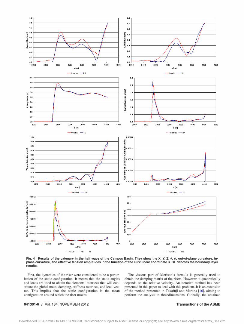
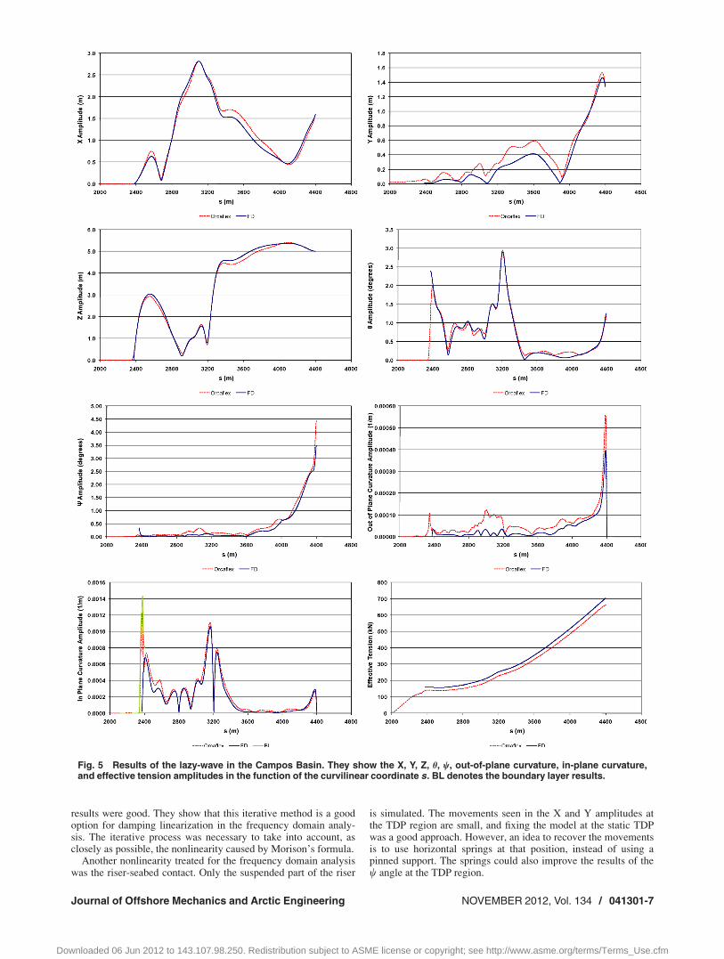
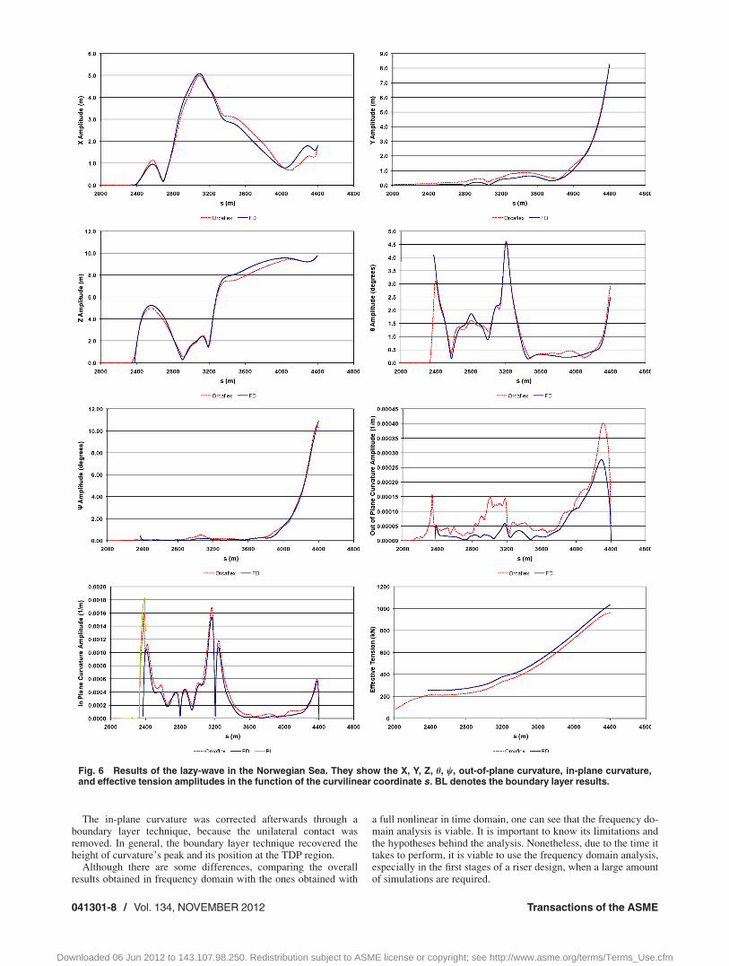
The results of all analyses compared to the results obtainedwith OrcaflexTM, which performs a full nonlinear analysis, areshown in Figs. 4, 5, and 6.

Table 1 Catenary’s properties

Segment 1

Diameter (m) 0.4064Weight in air (kN/m) 2.4927Bending stiffness (kN m2) 78,000Axial stiffness (kN) 4,000,000Torsional stiffness (kN m2) 60,000Length (m) 4440Drag coefficient 1.1Inertia coefficient 2

Table 2 Lazy-wave’s properties

Segment 1 Segment 2 Segment 3

Diameter (m) 0.4064 0.8 0.4064Weight in air (kN/m) 2.4927 3.9044 2.4927Bending stiffness (kN m2) 78,000 78,000 78,000Axial stiffness (kN) 4,000,000 4,000,000 4,000,000Torsional stiffness (kN m2) 60,000 60,000 60,000Length (m) 2800 400 1200Drag coefficient 1.1 1.1 1.1Inertia coefficient 2 2 2

Table 3 Geometrical and environmental data

Geometry Xtop (m) 3800Ztop (m) 1255

Environment Depth (m) 1255Water density (t/m3) 1.024

Gravity acceleration (m/s2) 9.807

Table 4 Wave and top motion for the Campos Basin

Period 13.0 sWave Height 8.0 m

Angle 90 degX Movement Amplitude 1.601 m

Phase 75.8112 degY Movement Amplitude 1.3383 m

Phase �14.9582 degZ Movement Amplitude 4.9996 m

Phase 58.9947 deg

041301-4 / Vol. 134, NOVEMBER 2012 Transactions of the ASME

Downloaded 06 Jun 2012 to 143.107.98.250. Redistribution subject to ASME license or copyright; see http://www.asme.org/terms/Terms_Use.cfm

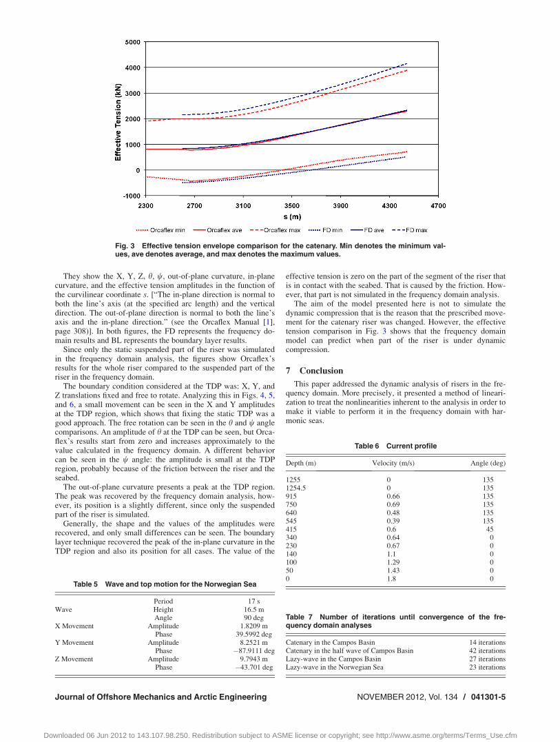
They show the X, Y, Z, h, w, out-of-plane curvature, in-planecurvature, and the effective tension amplitudes in the function ofthe curvilinear coordinate s. [“The in-plane direction is normal toboth the line’s axis (at the specified arc length) and the verticaldirection. The out-of-plane direction is normal to both the line’saxis and the in-plane direction.” (see the Orcaflex Manual [1],page 308)]. In both figures, the FD represents the frequency do-main results and BL represents the boundary layer results.

Since only the static suspended part of the riser was simulatedin the frequency domain analysis, the figures show Orcaflex’sresults for the whole riser compared to the suspended part of theriser in the frequency domain.

The boundary condition considered at the TDP was: X, Y, andZ translations fixed and free to rotate. Analyzing this in Figs. 4, 5,and 6, a small movement can be seen in the X and Y amplitudesat the TDP region, which shows that fixing the static TDP was agood approach. The free rotation can be seen in the h and w anglecomparisons. An amplitude of h at the TDP can be seen, but Orca-flex’s results start from zero and increases approximately to thevalue calculated in the frequency domain. A different behaviorcan be seen in the w angle: the amplitude is small at the TDPregion, probably because of the friction between the riser and theseabed.

The out-of-plane curvature presents a peak at the TDP region.The peak was recovered by the frequency domain analysis, how-ever, its position is a slightly different, since only the suspendedpart of the riser is simulated.

Generally, the shape and the values of the amplitudes wererecovered, and only small differences can be seen. The boundarylayer technique recovered the peak of the in-plane curvature in theTDP region and also its position for all cases. The value of the

effective tension is zero on the part of the segment of the riser thatis in contact with the seabed. That is caused by the friction. How-ever, that part is not simulated in the frequency domain analysis.

The aim of the model presented here is not to simulate thedynamic compression that is the reason that the prescribed move-ment for the catenary riser was changed. However, the effectivetension comparison in Fig. 3 shows that the frequency domainmodel can predict when part of the riser is under dynamiccompression.

7 Conclusion

This paper addressed the dynamic analysis of risers in the fre-quency domain. More precisely, it presented a method of lineari-zation to treat the nonlinearities inherent to the analysis in order tomake it viable to perform it in the frequency domain with har-monic seas.

Fig. 3 Effective tension envelope comparison for the catenary. Min denotes the minimum val-ues, ave denotes average, and max denotes the maximum values.

Table 5 Wave and top motion for the Norwegian Sea

Period 17 sWave Height 16.5 m

Angle 90 degX Movement Amplitude 1.8209 m

Phase 39.5992 degY Movement Amplitude 8.2521 m

Phase �87.9111 degZ Movement Amplitude 9.7943 m

Phase �43.701 deg

Table 6 Current profile

Depth (m) Velocity (m/s) Angle (deg)

1255 0 1351254.5 0 135915 0.66 135750 0.69 135640 0.48 135545 0.39 135415 0.6 45340 0.64 0230 0.67 0140 1.1 0100 1.29 050 1.43 00 1.8 0

Table 7 Number of iterations until convergence of the fre-quency domain analyses

Catenary in the Campos Basin 14 iterationsCatenary in the half wave of Campos Basin 42 iterationsLazy-wave in the Campos Basin 27 iterationsLazy-wave in the Norwegian Sea 23 iterations

Journal of Offshore Mechanics and Arctic Engineering NOVEMBER 2012, Vol. 134 / 041301-5

Downloaded 06 Jun 2012 to 143.107.98.250. Redistribution subject to ASME license or copyright; see http://www.asme.org/terms/Terms_Use.cfm

First, the dynamics of the riser were considered to be a pertur-bation of the static configuration. It means that the static anglesand loads are used to obtain the elements’ matrices that will con-stitute the global mass, damping, stiffness matrices, and load vec-tor. This implies that the static configuration is the meanconfiguration around which the riser moves.

The viscous part of Morison’s formula is generally used toobtain the damping matrix of the risers. However, it quadraticallydepends on the relative velocity. An iterative method has beenpresented in this paper to deal with this problem. It is an extensionof the method presented in Takafuji and Martins [16], aiming toperform the analysis in threedimensions. Globally, the obtained

Fig. 4 Results of the catenary in the half wave of the Campos Basin. They show the X, Y, Z, h, w, out-of-plane curvature, in-plane curvature, and effective tension amplitudes in the function of the curvilinear coordinate s. BL denotes the boundary layerresults.

041301-6 / Vol. 134, NOVEMBER 2012 Transactions of the ASME

Downloaded 06 Jun 2012 to 143.107.98.250. Redistribution subject to ASME license or copyright; see http://www.asme.org/terms/Terms_Use.cfm

results were good. They show that this iterative method is a goodoption for damping linearization in the frequency domain analy-sis. The iterative process was necessary to take into account, asclosely as possible, the nonlinearity caused by Morison’s formula.

Another nonlinearity treated for the frequency domain analysiswas the riser-seabed contact. Only the suspended part of the riser

is simulated. The movements seen in the X and Y amplitudes atthe TDP region are small, and fixing the model at the static TDPwas a good approach. However, an idea to recover the movementsis to use horizontal springs at that position, instead of using apinned support. The springs could also improve the results of thew angle at the TDP region.

Fig. 5 Results of the lazy-wave in the Campos Basin. They show the X, Y, Z, h, w, out-of-plane curvature, in-plane curvature,and effective tension amplitudes in the function of the curvilinear coordinate s. BL denotes the boundary layer results.

Journal of Offshore Mechanics and Arctic Engineering NOVEMBER 2012, Vol. 134 / 041301-7

Downloaded 06 Jun 2012 to 143.107.98.250. Redistribution subject to ASME license or copyright; see http://www.asme.org/terms/Terms_Use.cfm

The in-plane curvature was corrected afterwards through aboundary layer technique, because the unilateral contact wasremoved. In general, the boundary layer technique recovered theheight of curvature’s peak and its position at the TDP region.

Although there are some differences, comparing the overallresults obtained in frequency domain with the ones obtained with

a full nonlinear in time domain, one can see that the frequency do-main analysis is viable. It is important to know its limitations andthe hypotheses behind the analysis. Nonetheless, due to the time ittakes to perform, it is viable to use the frequency domain analysis,especially in the first stages of a riser design, when a large amountof simulations are required.

Fig. 6 Results of the lazy-wave in the Norwegian Sea. They show the X, Y, Z, h, w, out-of-plane curvature, in-plane curvature,and effective tension amplitudes in the function of the curvilinear coordinate s. BL denotes the boundary layer results.

041301-8 / Vol. 134, NOVEMBER 2012 Transactions of the ASME

Downloaded 06 Jun 2012 to 143.107.98.250. Redistribution subject to ASME license or copyright; see http://www.asme.org/terms/Terms_Use.cfm

References

[1] Orcina, 2010, “OrcaFlex Manual Version 9.4a,” Daltongate, Ulverston,Cumbria, UK.

[2] Patel, M. H., and Seyed, F. B., 1995, “Review of Flexible Riser Modelling andAnalysis Techniques,” Eng. Struct., 17(4), pp. 293–304.

[3] Santos, M. F., 2003, “Three-Dimensional Global Mechanics of SubmergedCables,” PhD thesis, University of Sao Paulo, Sao Paulo, Brazil (in Portuguese).

[4] Silveira, L. M. Y., and Martins, C. A., 2004, “A Numerical Method to Solve theStatic Problem of a Catenary Riser,” Proceedings of the 23rd International Con-ference on Offshore Mechanics and Arctic Engineering (OMAE), Canada.

[5] Silveira, L. M. Y., and Martins, C. A., 2005, “A Numerical Method to Solve theThree-Dimensional Static Problem of a Riser With Bending Stiffness,” Pro-ceedings of the 24th International Conference on Offshore Mechanics and Arc-tic Engineering (OMAE), Greece.

[6] Aranha, J. A. P., Martins, C. A., and Pesce, C. P., 1997, “Analytical Approxi-mation for the Dynamic Bending Moment at the Touchdown Point of a Cate-nary Riser,” Int. J. Offshore Polar Eng., 7(4), pp. 293–300.

[7] Keller, H. B., 1968, Numerical Methods for Two-Point Boundary Value Prob-lems, Blaisdell, Waltham, MA.

[8] Martins, C. A., 1998, “Poliflex – Poliflex User’s Manual,” EPUSP, Sao Paulo(in Portuguese).

[9] Morison, J. R., O’Brian, M. P., Johnson, J. W., and Schaaf, S. A., 1950, “TheForce Exerted by Surface Waves on Piles,” Trans. Am. Inst. Min., Metall. Pet.Eng., 189, pp. 149–154.

[10] Dantas, C. M. S., Siqueira, M. Q., Ellwanger, G. B., Torres, A. L. F. L., andMourelle, M. M., 2004, “A Frequency Domain Approach for Random Fatigue

Analysis of Steel Catenary Risers at Brazil’s Deep Waters,” Proceedings of the23rdInternational Conference on Offshore Mechanics and Arctic Engineering(OMAE), Canada.

[11] Gudmestad, O. T., and Connor, J. J., 1983, “Linearization Methods and theInfluence of Current on the Nonlinear Hydrodynamic Drag Force,” Appl. OceanRes., 5(4), pp. 184–194.

[12] Langley, R. S., 1984, “The Linearisation of Three Dimensional Drag Force inRandom Seas With Current,” Appl. Ocean Res., 6(3), pp. 126–131.

[13] Leira, B. J., 1987, “Multidimensional Stochastic Linearisation of Drag Forces,”Appl. Ocean Res., 9(3), pp. 150–162.

[14] Chen, Y. H., and Lin, F. M., 1989, “General Drag-Force Linearization for Non-linear Analysis of Marine Risers,” Ocean Eng., 16(3), pp. 265–280.

[15] Liu, Y., and Bergdahl, L., 1997, “Frequency-domain Dynamic Analysis ofCables,” Eng. Struct., 19(6), pp. 499–506.

[16] Martins, C. A., 2000, “A Tool to the Viability Study of Steel Catenary Risers,”Habilitation thesis, University of Sao Paulo, Sao Paulo, Brazil (in Portuguese).

[17] Takafuji, F. C. M., and Martins, C. A., 2007, “Damping Linearization for Fre-quency Domain Lazy-Wave Riser Analysis,” Proceedings of the 17th Interna-tional Offshore and Polar Engineering Conference, Lisbon, Portugal.

[18] Takafuji, F. C. M., 2010, “Three-Dimensional Riser Dynamics,” PhD thesis,University of Sao Paulo, Sao Paulo, Brazil (in Portuguese).

[19] Teng, B., and Li, Y. C., 1990, “The Linearization of Drag Force and the ErrorEstimation of Linear Force Spectrum,” Coastal Eng., 14, pp. 173–183.

[20] Det Norsk Veritas, 2010, “Position Mooring,” Recommended Practice ReportNo. DNV-OS-E301.

[21] Det Norsk Veritas, 2006, “Free Spanning Pipelines,” Recommended PracticeReport No. DNV-RP-F105.

Journal of Offshore Mechanics and Arctic Engineering NOVEMBER 2012, Vol. 134 / 041301-9

Downloaded 06 Jun 2012 to 143.107.98.250. Redistribution subject to ASME license or copyright; see http://www.asme.org/terms/Terms_Use.cfm