Comparison between thick level set (TLS) and cohesive zone modelsAndrés Parrilla Gómez1, Nicolas Moës1* and Claude Stolz1,2
BackgroundModeling the failure of quasi-brittle structures is an important aim of numerical simula-tions. Two main kind of models have been developed [1]: crack based ones, as the cohe-sive zone model, and damage based ones. The first ones deals with crack evolution in elastic materials whereas damage models consider a continuous transition from sound to totally damaged materials.
Quasi-brittle structures are characterized by the existence of a non-negligible fracture process zone. Linear elasticity fracture mechanics (LEFM) does not apply as it requires this zone to be negligible. In cohesive zone models (CZM), it is assumed that the process zone is concentrated over a line (2D problems) or a surface (3D), that defines the crack
Abstract
Background: Two main families of methods exist to model failure of quasi-brittle structures. The first one consists on crack based models, like cohesive zone models. The second one is a continuum damage approach that leads to a local loss of stiffness. Local damage models need some regularization in order to avoid spurious localization. A recent one, the thick level set damage model, bridges both families by using level-sets. Cohesive and TLS models are presented. The cohesive one represents quasi-brittle behaviors with good accuracy but requires extra equations to determine the crack path. The TLS has proved its capability to model complex crack paths while easily rep-resenting cracks (i.e. displacement jumps); contrary to most damage models.
Methods: A one-dimensional analytical relationship is exhibited between TLS and cohesive models. The local damage behavior needed to obtain the same global behav-ior of a bar than with cohesive model is derived. It depends on the choice of some TLS parameters, notably the characteristic length ℓc. This local behavior is applied to bi-dimensional simulations of three point bending as well as mixed-mode single edge notched specimens are performed. Results are compared to cohesive simulations, regarding both crack paths and force-CMOD curves.
Results: Force-CMOD curves obtained are very similar with both models. Theoretical analysis in 1D and numerical results in 2D indicates that, as ℓc goes to zero, TLS results tend to CZM ones.
Conclusions: The TLS model yields very similar results to the cohesive one, without the need for extra equations to determine the crack path.
Keywords: Damage mechanics, Thick level set, Cohesive zone, X-FEM, Level-set, Three point bending, Single edge notch
Parrilla Gómez et al. Adv. Model. and Simul. in Eng. Sci. (2015) 2:18 DOI 10.1186/s40323-015-0041-9
*Correspondence: [email protected] 1 GeM, UMR CNRS 6183, Ecole Centrale de Nantes, 1 rue de la Noë, 44321 Nantes, FranceFull list of author information is available at the end of the article
Page 2 of 22Parrilla Gómez et al. Adv. Model. and Simul. in Eng. Sci. (2015) 2:18
path. Damage models make no strong assumption on its size and shape; damaged zone length and width are a priori not negligible compared to the size of the material domain.
The CZM definition needs to know the crack path. If it is unknown, LEFM based methods exist to predict it. Even if most cohesive models cannot handle complex crack paths, such as branching, some adaptations [2, 3] allow to do so. Regarding damage models, there exist different families. Indeed, purely local damage presents spurious localization and different regularization methods have been proposed: strain or damage averaging, higher-order gradient, phase-field, variational models... These models are able to deal with complex damaged zone shape evolution but present important difficulties to deal with jump in displacement. Moreover, as damage evolution law has to be enforced over the whole material domain, computational cost is more important than for cohesive models.
The crack band model [4] is an intermediate between the cohesive model and classical damage ones, as damage is represented as a non-linear behavior of some elements that defines the crack path. However, damage band width is only dependent on the chosen elements that have a non-linear behavior and the crack path has to be previously deter-mined. More recently, a level-set based damage model, the thick level set (TLS) model, has been presented [5]. This damage model bridges both families of models as it is able to recover complex crack paths while introducing jumps in displacement in a natural way. Contrary to the crack band model, the width of the damage band is here a param-eter that is not related to the mesh.
The goal of this paper is to establish a one-dimensional equivalence between the cohe-sive zone model and a damage model with TLS regularization. Note that similar analysis concerning cohesive and gradient damage models has been performed by Lorentz in [6]. Thus, based on this equivalence, a method to derive a local damage behavior to use in TLS from any cohesive behavior will be exhibited. Later, it will be used in two-dimen-sional simulations and results will be compared to classical cohesive simulations, that have proved their capability to reproduce experimental results.
We consider structures under quasi-static load. We restrict the study to small strain and displacement and no particular shear behavior is considered, unlike in [7]. The rela-tionship between cohesive and TLS models is analyzed. A one-dimensional equivalence is analytically first established. Then, these results are used to compare two-dimensional behaviors.
Let us start with the one-dimensional comparison between the cohesive and the TLS models. We consider an elastic bar of length 2L: x ∈ [−L, L] and Young modulus E. Deg-radation in this bar will be modeled either with a cohesive zone located at x = 0 or with an evolving damage layer centered at x = 0. Due to symmetry, only half of the bar needs to be considered: x ∈ [0, L]. Let u(x) denote the displacement along the bar and in par-ticular u(L) = uL the displacement of the extremity. The stress σ is here a scalar variable.
In the cohesive zone model, the displacement at x = 0 is discontinuous and the cohe-sive zone opening is given by w = 2u(0+). Regarding the TLS model, the extent of the damage layer over the half-bar is denoted by [0, l] where x = l corresponds to the cur-rent damage front location. An example of the displacement u(x) for both cohesive and TLS models is shown in Fig. 1.
Page 3 of 22Parrilla Gómez et al. Adv. Model. and Simul. in Eng. Sci. (2015) 2:18
Cohesive zone model
The cohesive zone model was first introduced by Dugdale in [8] for ductile materials and by Barenblatt in [9] for concrete. The model represents the progressive fracture process by condensing over a crack the effect of the whole fracture process zone. A cohesive behavior is imposed between the crack lips (see Fig. 2a). The bi-linear cohesive law, well-known for concrete behavior, is presented in Fig. 3a. This model is widely used [1] and is considered to have good capabilities to fit experimental results when the crack path is known. If it is not previously known, a complementary method, like the maximum tan-gential stress (MTS) criterion [10], has to be applied.
Let us consider the following free energy of the cohesive zone, located at x = 0.
where k > 0 and gCZM is a decreasing dimensionless function that characterizes the stiffness of the cohesive zone. We derive the dual quantities t (tension) and A
(1)�CZM(w,α) =1
2gCZM(α)kw2
(2)σ =∂�CZM
∂w= gCZM(α)kw
−L −l 0 l L
w
position xdisplacementu(x)
TLSCZM
Fig. 1 Displacement over the whole bar for CZM and TLS models for a partially damaged bar. L is the length of the bar and l the position of the damage front in TLS model.
σ
a Cohesive zone. b Thick level set model.
Fig. 2 Representation of an open crack with a cohesive zone (left) and with a TLS damage zone (right). Dark (light) gray indicates (un) damaged.
Page 4 of 22Parrilla Gómez et al. Adv. Model. and Simul. in Eng. Sci. (2015) 2:18
The evolution of α is governed by the criterion fCZM(A,α) = A− Ac(α) with the associ-ated law:
where Ac(α) is supposed to be finite for all α.The model depends on two functional parameters: gCZM(α) and Ac(α). When they are
known, and assuming the uniqueness of evolution of α for any opening history, we can derive a tension-opening curve f that describes the tension of the cohesive zone under a monotonously increasing opening w. We will denote by F the corresponding dimension-less function:
The relation between gCZM, Ac and f writes from (2), (3), (4) and (5):
Here, we will only consider cohesive behaviors with infinite initial stiffness and null stiff-ness for α = 1 (see Fig. 4), that is
We define two characteristic values: σf and wf
(3)A =−∂�CZM
∂α= −
1
2g ′CZM(α)kw2
(4)fCZM(A,α) ≤ 0, α ≥ 0 and fCZM(A,α)α = 0
(5)σ = f (w)
(6)∀α, kgCZM(α)
√
−2Ac(α)
kg ′CZM(α)= f
(√
−2Ac(α)
kg ′CZM(α)
)
(7)limα→0+
gCZM(α) = +∞ and gCZM(1) = 0
(8)wf = limα→1−
w(α) = limα→1−
√
−2Ac(α)
kg ′CZM(α)
w
σ
wfw1wk
σf
σk
σ2
σf
ε
σlc =15 mm
lc =30 mm
lc =60 mm
lc =100 mm
a Cohesive bi-linear law. b TLS equivalent local behavior for different �c values.
Fig. 3 Cohesive bi-linear law and TLS local behavior for different ℓc.
Page 5 of 22Parrilla Gómez et al. Adv. Model. and Simul. in Eng. Sci. (2015) 2:18
which are supposed to be finite. Thus, as gCZM(α) is monotonous, (7) implies
We denote by F the dimensionless cohesive function depicted on Fig. 4 and associated to f by
Thick level set damage model
The bar is made of a material with the following free energy density
where gdam is a decreasing dimensionless function respecting gdam(0) = 1 that charac-terizes the remaining stiffness for a given amount of damage d. We can derive the stress σ and the local energy release rate Y
We can write a local damage evolution criterion fdam(Y , d) = Y − h(d)Yc and an associ-ated law:
(9)σf = limα→0+
σ(α) = limα→0+
(
gCZM(α)
√
−2kAc(α)
g ′CZM(α)
)
(10)limα→0+
g ′CZM(α) = −∞ and limα→0+
w(α) = 0
(11)σ = f (w) = σf F
(
w
wf
)
(12)�dam(ε, d) =1
2gdam(d)Eε
2
(13)Y =∂�dam
∂ε= −
1
2gdam(d)Eε
(14)Y = −∂�dam
∂d= −
1
2g ′dam(d)Eε
2
(15)fdam(Y , d) ≤ 0, d ≥ 0 and fdam(Y , d)d = 0
α ↗
α = 0
α = 1
w/wf
σ/σf
1
1
00
Fig. 4 Response of a typical cohesive zone model for an imposed increasing crack opening.
Page 6 of 22Parrilla Gómez et al. Adv. Model. and Simul. in Eng. Sci. (2015) 2:18
Yc is a constant. The dependence on d of the critical energy release rate is concentrated on the dimensionless function h(d). The interest of making the critical energy release rate depend on d has been shown in [11, 12].
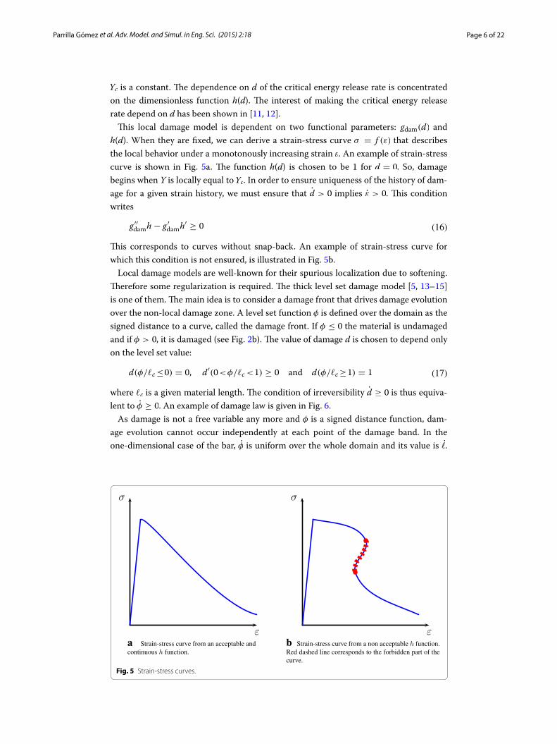
This local damage model is dependent on two functional parameters: gdam(d) and h(d). When they are fixed, we can derive a strain-stress curve σ = f (ε) that describes the local behavior under a monotonously increasing strain ε. An example of strain-stress curve is shown in Fig. 5a. The function h(d) is chosen to be 1 for d = 0. So, damage begins when Y is locally equal to Yc. In order to ensure uniqueness of the history of dam-age for a given strain history, we must ensure that d > 0 implies ε > 0. This condition writes
This corresponds to curves without snap-back. An example of strain-stress curve for which this condition is not ensured, is illustrated in Fig. 5b.
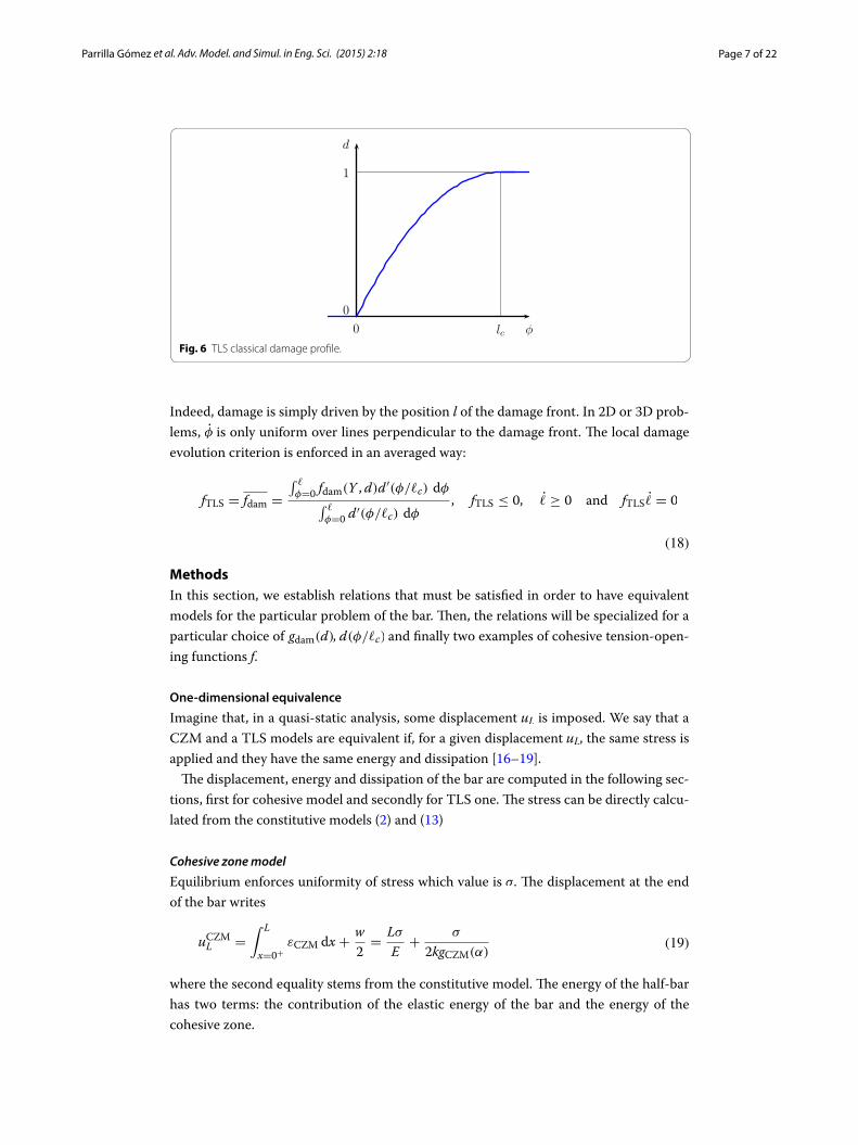
Local damage models are well-known for their spurious localization due to softening. Therefore some regularization is required. The thick level set damage model [5, 13–15] is one of them. The main idea is to consider a damage front that drives damage evolution over the non-local damage zone. A level set function φ is defined over the domain as the signed distance to a curve, called the damage front. If φ ≤ 0 the material is undamaged and if φ > 0, it is damaged (see Fig. 2b). The value of damage d is chosen to depend only on the level set value:
where ℓc is a given material length. The condition of irreversibility d ≥ 0 is thus equiva-lent to φ ≥ 0. An example of damage law is given in Fig. 6.
As damage is not a free variable any more and φ is a signed distance function, dam-age evolution cannot occur independently at each point of the damage band. In the one-dimensional case of the bar, φ is uniform over the whole domain and its value is ℓ.
(16)g ′′damh− g ′damh′ ≥ 0
(17)d(φ/ℓc≤0) = 0, d′(0<φ/ℓc<1) ≥ 0 and d(φ/ℓc≥1) = 1
σ
εa Strain-stress curve from an acceptable andcontinuous h function.
σ
εb Strain-stress curve from a non acceptable h function.Red dashed line corresponds to the forbidden part of thecurve.
Fig. 5 Strain-stress curves.
Page 7 of 22Parrilla Gómez et al. Adv. Model. and Simul. in Eng. Sci. (2015) 2:18
Indeed, damage is simply driven by the position l of the damage front. In 2D or 3D prob-lems, φ is only uniform over lines perpendicular to the damage front. The local damage evolution criterion is enforced in an averaged way:
MethodsIn this section, we establish relations that must be satisfied in order to have equivalent models for the particular problem of the bar. Then, the relations will be specialized for a particular choice of gdam(d), d(φ/ℓc) and finally two examples of cohesive tension-open-ing functions f.
One‑dimensional equivalence
Imagine that, in a quasi-static analysis, some displacement uL is imposed. We say that a CZM and a TLS models are equivalent if, for a given displacement uL, the same stress is applied and they have the same energy and dissipation [16–19].
The displacement, energy and dissipation of the bar are computed in the following sec-tions, first for cohesive model and secondly for TLS one. The stress can be directly calcu-lated from the constitutive models (2) and (13)
Cohesive zone model
Equilibrium enforces uniformity of stress which value is σ. The displacement at the end of the bar writes
where the second equality stems from the constitutive model. The energy of the half-bar has two terms: the contribution of the elastic energy of the bar and the energy of the cohesive zone.
(18)
fTLS = fdam =
∫
ℓ
φ=0 fdam(Y , d)d′(φ/ℓc) dφ∫
ℓ
φ=0 d′(φ/ℓc) dφ
, fTLS ≤ 0, ℓ ≥ 0 and fTLSℓ = 0
(19)uCZML =
∫ L
x=0+εCZM dx +
w
2=
Lσ
E+
σ
2kgCZM(α)
d
φ
1
0lc0
Fig. 6 TLS classical damage profile.
Page 8 of 22Parrilla Gómez et al. Adv. Model. and Simul. in Eng. Sci. (2015) 2:18
The dissipation writes
Thick level set model
The same computations that have been done for the cohesive model are here performed for the TLS. Equilibrium leads to σ(x) = σ. The displacement at the end of the bar writes
The energy of the half-bar is
The dissipation writes
Let us remark that in the one-dimensional case of the bar, the TLS variable φ is related to the coordinate of a point of the bar x and the position of the damage front l by
Moreover, we remind for a better comprehension of the following developments that at the center of the bar (x = 0), the value of damage is d(ℓ/ℓc).
General relationships
We have determined the displacement uL, the total energy of the half-bar E and the dis-sipation D linked to the evolution of the internal variable (α or d) for both cohesive and TLS models. The equality of each one of these three quantities for both models leads to (26) and (27). In order to close the system, we need to remind the normality rule for one of the models (28). The second one is redundant.
(20)ECZM(u,w,α) =
∫ L
x=0+
1
2Eε(u)2 dx +
1
2�CZM(w,α) =
σ2L
2E+
σ2
4gCZM(α)k
(21)DCZM =1
2Aα =
1
2Ac(α)α
(22)uTLSL =
∫ L
x=0εTLS dx =
∫ L
0
σ
Egdam(d)dx
(23)ETLS(u, d) =
∫ L
x=0�dam(u, d) dx =
∫ L
x=0
σ2
2gdam(d)Edx
(24)DTLS(Y , d) =
∫ L
x=0Y d dx = Ycℓ
∫
ℓ
φ=0h(d)
d′(φ/ℓc)
ℓcdφ
(25)φ = ℓ− x
(26)1
2kgCZM(α)=
1
E
∫
ℓ
φ=0
(
1
gdam(d(φ/ℓc))− 1
)
dφ
(27)1
2Ac(α)α = Ycℓ
∫ d(ℓ/ℓc)
d=0h(d) dd
(28)Ac(α)α =−σ2
2k
g ′CZM(α)
g2CZM(α)α
Page 9 of 22Parrilla Gómez et al. Adv. Model. and Simul. in Eng. Sci. (2015) 2:18
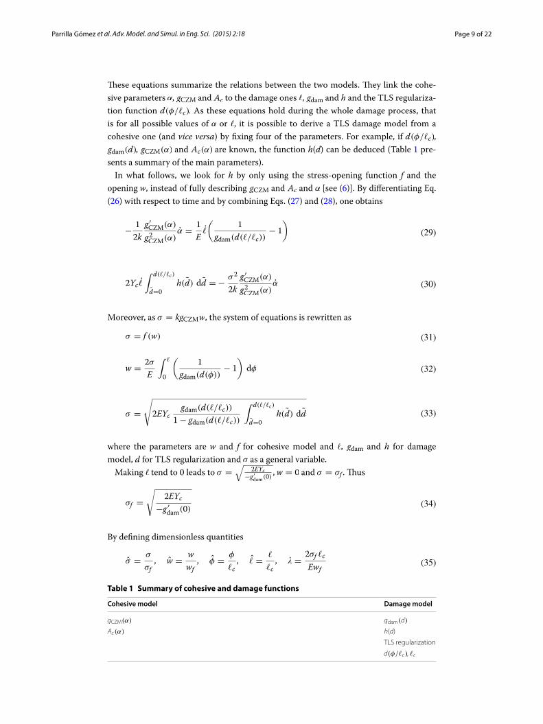
These equations summarize the relations between the two models. They link the cohe-sive parameters α, gCZM and Ac to the damage ones ℓ, gdam and h and the TLS regulariza-tion function d(φ/ℓc). As these equations hold during the whole damage process, that is for all possible values of α or ℓ, it is possible to derive a TLS damage model from a cohesive one (and vice versa) by fixing four of the parameters. For example, if d(φ/ℓc), gdam(d), gCZM(α) and Ac(α) are known, the function h(d) can be deduced (Table 1 pre-sents a summary of the main parameters).
In what follows, we look for h by only using the stress-opening function f and the opening w, instead of fully describing gCZM and Ac and α [see (6)]. By differentiating Eq. (26) with respect to time and by combining Eqs. (27) and (28), one obtains
Moreover, as σ = kgCZMw, the system of equations is rewritten as
where the parameters are w and f for cohesive model and ℓ, gdam and h for damage model, d for TLS regularization and σ as a general variable.
Making ℓ tend to 0 leads to σ =√
2EYc−g ′dam(0)
, w = 0 and σ = σf . Thus
By defining dimensionless quantities
(29)−1
2k
g ′CZM(α)
g2CZM(α)α =
1
Eℓ
(
1
gdam(d(ℓ/ℓc))− 1
)
(30)2Ycℓ
∫ d(ℓ/ℓc)
d=0h(d) dd =−
σ2
2k
g ′CZM(α)
g2CZM(α)α
(31)σ = f (w)
(32)w =2σ
E
∫
ℓ
0
(
1
gdam(d(φ))− 1
)
dφ
(33)σ =
√
2EYcgdam(d(ℓ/ℓc))
1− gdam(d(ℓ/ℓc))
∫ d(ℓ/ℓc)
d=0h(d) dd
(34)σf =
√
2EYc
−g ′dam(0)
(35)σ =σ
σf, w =
w
wf, φ =
φ
ℓc, ℓ =
ℓ
ℓc, � =
2σf ℓc
Ewf
Table 1 Summary of cohesive and damage functions
Cohesive model Damage model
gCZM(α) gdam(d)
Ac(α) h(d)
TLS regularization
d(φ/ℓc), ℓc
Page 10 of 22Parrilla Gómez et al. Adv. Model. and Simul. in Eng. Sci. (2015) 2:18
and
the system (31), (32) and (33) can be written in a dimensionless and condensed form
These equations hold for all dimensionless position of the damage front in the bar ℓ, and therefore for any value of φ. Using φ instead of ℓ gives a more general formulation, not constrained to the bar case.
Meaning of �
The dimensionless quantity � includes the main parameters of both models and in par-ticular the TLS characteristic length ℓc. Different lengths have been defined to charac-terize the size of the fracture process zone [20–22] in quasi-brittle materials. For the specific case of cohesive models, Smith estimated its length ℓcoh in [23] for a crack evolv-ing in an infinite body and for a large range of cohesive laws:
Thus, the parameter � is close to the ratio between damage band width and cohesive zone length (see Fig. 7).
(36)I(ℓ) =
∫
ℓ
0
1− gdam(d(φ))
gdam(d(φ))dφ,
(37)σ = F(�I σ ) and
∫
ℓ
φ=0h(d) dφ = −g ′dam(0)
1− gdam(d(ℓ))
gdam(d(ℓ))σ2
(38)σ = F(�I σ ) and
∫
φ
0h(φ) dφ = −g ′dam(0)
1− gdam(d(φ))
gdam(d(φ))σ2
(39)ℓcoh ≈3
2
Ewf
2σf
(40)� ≈3
2
ℓc
ℓcoh
2 �c
�coh
Fig. 7 Classical shape of a damaged zone and lengths definitions.
Page 11 of 22Parrilla Gómez et al. Adv. Model. and Simul. in Eng. Sci. (2015) 2:18
The value of � will be chosen to be less than 12. Indeed, as it is explained in "Appendix 2", the condition of uniqueness of the solution enforces values of � that are close or smaller than 12. It corresponds to the choice of a small enough damage band width in comparison to the fracture process length. Writing � � 1
2 and Eq. (40) leads to
From general to particular relations
These general relations are now derived in the case of a particular choice of gdam(d). Later, a particular form of d(φ) is assumed. Finally, the equations are particularized for two cohesive softening functions F: the linear and the bi-linear ones.
A choice of damage function gdamA classical choice is made:
The admissibility condition (16) becomes
and
The system of Eq. (38) can be rewritten as follows.
Moreover,
A choice of TLS damage profile d(φ)
We consider a parabolic damage law (see Fig. 6)
and
(41)ℓc �1
3ℓcoh
(42)gdam(d) = 1− d, and then �dam(ε, d) =1
2(1− d)Eε2
(43)h′(d) ≥ 0
(44)I(φ) =
∫
φ
0
d
1− ddφ
(45)σ = F(�I σ ) and
∫
φ
0h(φ) dφ =
d(φ)
1− d(φ)σ2
(46)σf =√
2EYc
(47)d(φ) = 2φ − φ2
(48)I(φ) =φ2
1− φ
Page 12 of 22Parrilla Gómez et al. Adv. Model. and Simul. in Eng. Sci. (2015) 2:18
The system (45) writes now
This choice is motivated by a damage distribution obtained from non-local damage and fracture equivalence [18], damage profiles obtained by lattice model simulations [24] and their similarity with some acoustic emission profiles [25, 26].
Two examples of cohesive laws
Two particular cases of cohesive stress-opening functions are derived from previous relationships: the linear and the bi-linear ones.
Linear cohesive law
We consider first a linear cohesive law F(w) = 1− w (see Fig. 8). The softening function is obtained by (49).
Bi‑linear cohesive law
The bi-linear cohesive law is considered as it is one of the most popular laws to describe concrete [27–32]. It is presented in Fig. 3a. The method to obtain h is the same as pre-viously. The result is a discontinuous and increasing h function. Corresponding strain-stress curves are shown in Fig. 3b. All of them present a discontinuity that appears as a linear zone where strain and stress increase while damage value remains constant.
(49)σ = F
(
�φ2
1− φσ
)
and
∫
φ
0h(φ) dφ =
2φ − φ2
(φ − 1)2σ2
(50)σ (φ) =1− φ
1− φ + �φ2and
∫
φ
0h(φ) dφ =
2φ − φ2
(1− φ + �φ2)2
w
σ
wf
σf
a Cohesive linear law.
σf
ε
σ
lc
b TLS equivalent local behavior for different �c values.Increasing values of �c are indicated by the arrow.
Fig. 8 Cohesive linear law and TLS local behavior.
Page 13 of 22Parrilla Gómez et al. Adv. Model. and Simul. in Eng. Sci. (2015) 2:18
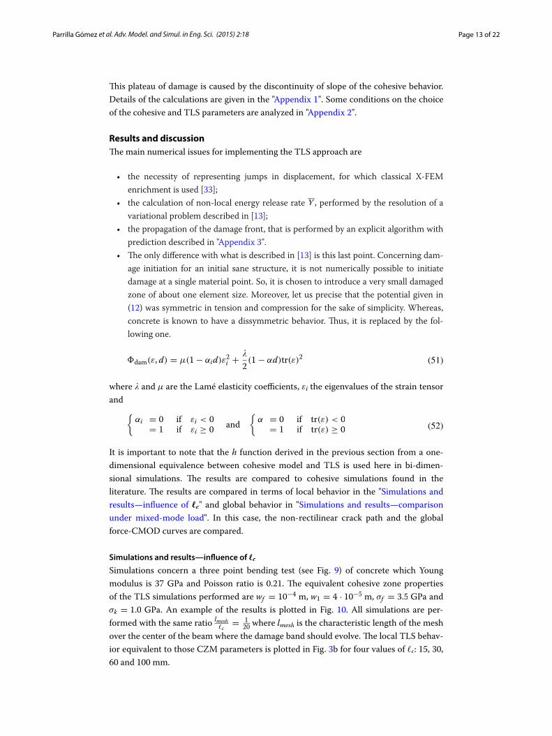
This plateau of damage is caused by the discontinuity of slope of the cohesive behavior. Details of the calculations are given in the "Appendix 1". Some conditions on the choice of the cohesive and TLS parameters are analyzed in "Appendix 2".
Results and discussionThe main numerical issues for implementing the TLS approach are
• the necessity of representing jumps in displacement, for which classical X-FEM enrichment is used [33];
• the calculation of non-local energy release rate Y , performed by the resolution of a variational problem described in [13];
• the propagation of the damage front, that is performed by an explicit algorithm with prediction described in "Appendix 3".
• The only difference with what is described in [13] is this last point. Concerning dam-age initiation for an initial sane structure, it is not numerically possible to initiate damage at a single material point. So, it is chosen to introduce a very small damaged zone of about one element size. Moreover, let us precise that the potential given in (12) was symmetric in tension and compression for the sake of simplicity. Whereas, concrete is known to have a dissymmetric behavior. Thus, it is replaced by the fol-lowing one.
where � and µ are the Lamé elasticity coefficients, εi the eigenvalues of the strain tensor and
It is important to note that the h function derived in the previous section from a one-dimensional equivalence between cohesive model and TLS is used here in bi-dimen-sional simulations. The results are compared to cohesive simulations found in the literature. The results are compared in terms of local behavior in the "Simulations and results—influence of ℓc" and global behavior in "Simulations and results—comparison under mixed-mode load". In this case, the non-rectilinear crack path and the global force-CMOD curves are compared.
Simulations and results—influence of ℓcSimulations concern a three point bending test (see Fig. 9) of concrete which Young modulus is 37 GPa and Poisson ratio is 0.21. The equivalent cohesive zone properties of the TLS simulations performed are wf = 10−4 m, w1 = 4 · 10−5 m, σf = 3.5 GPa and σk = 1.0 GPa. An example of the results is plotted in Fig. 10. All simulations are per-formed with the same ratio lmesh
ℓc= 1
20 where lmesh is the characteristic length of the mesh over the center of the beam where the damage band should evolve. The local TLS behav-ior equivalent to those CZM parameters is plotted in Fig. 3b for four values of ℓc: 15, 30, 60 and 100 mm.
(51)�dam(ε, d) = µ(1− αid)ε2i +
�
2(1− αd)tr(ε)2
(52)
{
αi = 0 if εi < 0= 1 if εi ≥ 0
and
{
α = 0 if tr(ε) < 0= 1 if tr(ε) ≥ 0
Page 14 of 22Parrilla Gómez et al. Adv. Model. and Simul. in Eng. Sci. (2015) 2:18
Global behavior: three point bending tests It is interesting to observe global CMOD-force curves shown in Fig. 11. The CMOD is here defined as the relative displacement of two points symmetrically located at the bottom face of the beam and separated by a distance equal to the beam depth. The global behavior is very close for the four values of ℓc. The main difference is the value of the maximum load. However this difference is slight: the maximum gap to the mean value 24.6 kN is less than 3%.
Damage zone shape at maximum load It is interesting to analyze the shape of the dam-aged zone at the maximum load. For different ℓc values, the position of the damage front is drawn in Fig. 12. The width of that zone is wider as ℓc is bigger. It is consistent with the
x
y
Fig. 9 Three point bending (TPB) test.
Fig. 10 Damage over the deformed specimen at a given step of the simulation. Blue is undammaged mate-rial. Red is damage close to 1. The white locates the crack.
2 · 10−5 4 · 10−5 6 · 10−5 8 · 10−5 1 · 10−40
0.5
1
1.5
2
2.5·104
CMOD (m)
force(N
)
lc = 15 mmlc = 30 mmlc = 60 mmlc = 100 mm
Fig. 11 Global behavior of TLS simulations of TPB test for different ℓc. Raw data is drawn.
Page 15 of 22Parrilla Gómez et al. Adv. Model. and Simul. in Eng. Sci. (2015) 2:18
fact that in TLS, the width of the fracture process zone is driven by ℓc. For example, the width of the damaged zone corresponding to a propagating crack is 2ℓc. The length of the damaged zone ahead of the crack tip is significantly the same for all ℓc. The depth is in fact driven by the equivalent cohesive behavior. We can conclude in which concerns the fracture process zone that its length is probably the same that in cohesive simula-tions and its width, neglected in CZM, is now driven by TLS parameter ℓc.
Agreement of the damage model with local cohesive behavior Cohesive theoretical local behavior is compared to TLS simulated one. As the cohesive zone model is concentrated over a line and has no width, it is necessary to determine which TLS quantities, denoted σTLS and wTLS, are compared to CZM ones, that is σxx and w. All over the evolving zone
of the damage band, the stress and the opening are computed for different positions y. Let ymax be the maximum value of y where d > 0. For y < ymax, about 15 positions are analyzed for the four ℓc values.
It is chosen to take the value of the stress σxx on the damage front, for a given value of y. By denoting l(y) the width of the damage band at a given y and Sy the points of the damage band where d(x, y) > 0 and y is fixed (see Fig. 13),
Concerning the opening, it is necessary for TLS to consider the whole width of the dam-aged zone. So it is chosen to compare displacement, perpendicular to the crack lips, at the boundaries of Sy. Thus, an additional term has to be added to cohesive opening to have comparable quantities:
(53)σTLS
(y) = σxx
(
x =l(y)
2, y
)
(54)wCZM(y)+
∫
Sy
εCZMxx (x, y) dx can be compared to
∫
Sy
εTLSxx (x, y) dx
Fig. 12 Position of the damage front at the maximum load for different ℓc values.
Sy
x
y
Fig. 13 Definition of Sy.
Page 16 of 22Parrilla Gómez et al. Adv. Model. and Simul. in Eng. Sci. (2015) 2:18
where ∫
SyεCZMxx (x, y) dx is the displacement caused by the deformation of the sane matter
around the cohesive crack. We can write
Thus we define:
The opening-stress curves obtained for different characteristic lengths ℓc are shown in Fig. 14. It can be observed that scatter plot is close to the equivalent cohesive law for small values of ℓc. The TLS model behavior around the damaged zone tends to the cohe-sive one as ℓc gets smaller. Simulation for much smaller ℓc values is difficult. Indeed, as ℓc goes to zero, displacement and damage gradients become extremely high and are dif-ficult to capture numerically.
Simulations and results—comparison under mixed‑mode load
In order to verify the consistency of global results for both models, a mixed-mode test is performed on single edge notched specimens. As the crack path is not a priori known, the cohesive model is coupled with classical fracture model under MTS criterion. Con-cerning TLS, no modification or enhancement is needed. The test, initially described in [34], is simulated with a cohesive model in [35]. The damage front evolution during the simulation is shown in Fig. 15. Note that the gradient of damage is not parallel to the boundary of the domain, whereas it is for phase-field models [36].
A first TLS simulation is performed with the smallest initial damaged zone considered here, that is of radius 0.10 ℓc (see Fig. 16). It can be observed that the cohesive crack path is close to the TLS crack lips even if some differences exist. Concerning the load-CMOD curve, there is an overestimation of the maximum load and of the end of the post-peak curve. The experimental envelope given by [35] of the tests described in [34] is also drawn.
Fig. 14 Stress distribution in the process zone for TLS damage model with different ℓc. Abscissa is an equiva-lent cohesive displacement jump. The continuous black line is the cohesive bi-linear model.
Page 17 of 22Parrilla Gómez et al. Adv. Model. and Simul. in Eng. Sci. (2015) 2:18
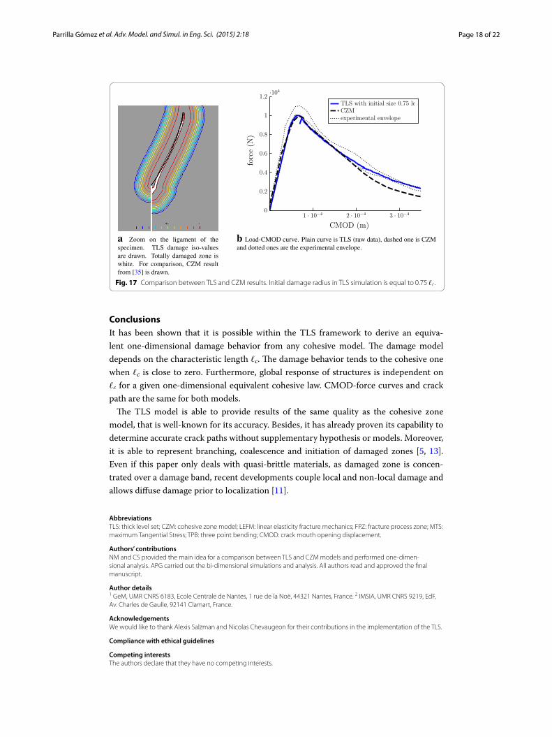
The cohesive model used in [35] forces the crack to be in the continuity of the notch. In the TLS model, no particular assumption is done on the damage zone path. This could explain the difference in the results presented in Fig. 16. To check this assumption, another TLS simulation is presented in Fig. 17, where initial damage is bigger than pre-viously. Here, its radius is 0.75ℓc. The CZM crack path is here overlapped with the TLS crack lips. Furthermore, load-CMOD curves are coincident until about the first half of the post-peak curve. Below that point, the TLS curve remains in the experimental enve-lope whereas cohesive one does not. It can be concluded that TLS simulation without an important initial damage give results slightly different from the CZM ones, but whose load-CMOD curve is closer to experimental one. Forcing similar crack paths by intro-ducing a more important initial damage leads to very close global results.
Fig. 15 Damage evolution in TLS simulation.
a Zoom on the ligament of thespecimen. TLS damage iso-valuesare drawn. Totally damaged zone iswhite. For comparison, CZM resultfrom [35] is drawn.
1 · 10−4 2 · 10−4 3 · 10−40
0.2
0.4
0.6
0.8
1
1.2·104
CMOD (m)
force(N
)
TLSCZMexperimental envelope
b Load-CMOD curve. Plain curve is TLS (raw data), dashed one is CZMand dotted ones are the experimental envelope.
Fig. 16 Comparison between TLS and CZM results. Initial damage radius in TLS simulation is equal to 0.10 ℓc.
Page 18 of 22Parrilla Gómez et al. Adv. Model. and Simul. in Eng. Sci. (2015) 2:18
ConclusionsIt has been shown that it is possible within the TLS framework to derive an equiva-lent one-dimensional damage behavior from any cohesive model. The damage model depends on the characteristic length ℓc. The damage behavior tends to the cohesive one when ℓc is close to zero. Furthermore, global response of structures is independent on ℓc for a given one-dimensional equivalent cohesive law. CMOD-force curves and crack path are the same for both models.
The TLS model is able to provide results of the same quality as the cohesive zone model, that is well-known for its accuracy. Besides, it has already proven its capability to determine accurate crack paths without supplementary hypothesis or models. Moreover, it is able to represent branching, coalescence and initiation of damaged zones [5, 13]. Even if this paper only deals with quasi-brittle materials, as damaged zone is concen-trated over a damage band, recent developments couple local and non-local damage and allows diffuse damage prior to localization [11].
AbbreviationsTLS: thick level set; CZM: cohesive zone model; LEFM: linear elasticity fracture mechanics; FPZ: fracture process zone; MTS: maximum Tangential Stress; TPB: three point bending; CMOD: crack mouth opening displacement.
Authors’ contributionsNM and CS provided the main idea for a comparison between TLS and CZM models and performed one-dimen-sional analysis. APG carried out the bi-dimensional simulations and analysis. All authors read and approved the final manuscript.
Author details1 GeM, UMR CNRS 6183, Ecole Centrale de Nantes, 1 rue de la Noë, 44321 Nantes, France. 2 IMSIA, UMR CNRS 9219, EdF, Av. Charles de Gaulle, 92141 Clamart, France.
AcknowledgementsWe would like to thank Alexis Salzman and Nicolas Chevaugeon for their contributions in the implementation of the TLS.
Compliance with ethical guidelines
Competing interestsThe authors declare that they have no competing interests.
a Zoom on the ligament of thespecimen. TLS damage iso-valuesare drawn. Totally damaged zone iswhite. For comparison, CZM resultfrom [35] is drawn.
1 · 10−4 2 · 10−4 3 · 10−40
0.2
0.4
0.6
0.8
1
1.2·104
CMOD (m)
force(N
)
TLS with initial size 0.75 lcCZMexperimental envelope
b Load-CMOD curve. Plain curve is TLS (raw data), dashed one is CZMand dotted ones are the experimental envelope.
Fig. 17 Comparison between TLS and CZM results. Initial damage radius in TLS simulation is equal to 0.75 ℓc.
Page 19 of 22Parrilla Gómez et al. Adv. Model. and Simul. in Eng. Sci. (2015) 2:18
AppendixAppendix 1: Bi‑linear cohesive law
We define the following dimensionless quantities
where wk = f −1(σk). By construction, we have the following relation
The tension opening relation is
For the first and second part of the law, we solve (49) for each part of the tension-open-ing function:
where
It remains to determine for which value φk of φ we move from the first to the second function. This value must ensure the continuity of H. Thus
with a =wk�σk
and φk between 0 and 1.
Appendix 2: Conditions on the parameters
It has been shown that h must verify condition (43) to ensure uniqueness of the solution. In the particular case of a linear cohesive model, uniqueness condition writes
If � >12, there exists a critical value φk above which h′ < 0 (corresponding to the red part
of the curve in Fig. 5b). It is difficult to obtain an explicit form of its value.Concerning bi-linear model, two parameters are defined
(57)w1 = w1/wf , wk = wk/wf , σk = σk/σf
(58)σk = 1− wk/w1
(59)σ = f (w) = 1− w/w1, 0 ≤ w ≤ wk
(60)σ = f (w) =σk
1− wk(1− w), wk ≤ w
(61)σ = 1− �σ I/w1 =1
1+ (�/w1)I⇒ H =
2φ − φ2
(1− φ + (�/w1)φ2)2
(62)σ =σk
1− wk
(1− �σ I) =σk/(1− wk )
1+ σk/(1− wk )�I⇒ H = (
σk
1− wk
)2
2φ − φ2
(1− φ +�σk
1−wk
φ2)2
(63)H(φ) =
∫
φ
0h(φ) dφ
(64)φk =a
2(
√
1+ 4/a− 1)
(65)� ≤1
2, it
Page 20 of 22Parrilla Gómez et al. Adv. Model. and Simul. in Eng. Sci. (2015) 2:18
The first one, �1, characterizes the first slope of the cohesive law and �2 the second one. Let us consider �1 > 1
2. Then, as seen above, there exists a critical value of φ that must not be exceeded. This value corresponds to a point of the cohesive law that must not be reached. If the position of the slope-discontinuity point is located before the criti-cal point, the condition h′ ≥ 0 is respected for the first part of the cohesive law. Finally, choosing �2 ≤ 1
2 ensures the condition for the whole local behavior. Some examples of equivalent one-dimensional strain-stress curves for a bi-linear cohesive law are shown in Fig. 8b.
Appendix 3: Damage evolution in TLS and load factor
We rewrite the evolution criterion (18) by defining the averaged quantities
where (s,φ) is a local basis, s a curvilinear abscissa of the front and ρ(s) the curvature of the damage front. Let fn denote the evolution criterion (18) at a given time step n
where Yn is the local release rate at the same iteration for a unitary load and µn is the load factor. The load factor at step n is computed in order to have
where Ŵ is the damage front. Thus
According to (18), only a single point of the front would evolve. However, as moving a single point of the front is not possible for a time-discretised problem [13], it is chosen to predict fn+1 and to apply a discretised version of the evolution law (18):
and we impose
where �φmax is chosen to be about 0.25 of the mesh characteristic length and
(66)�1 =
2σf ℓc
Ew1, �2 =
2σ2ℓc
Ewf=
2σkℓc
E(wf − wk)
(67)Y =
∫
ℓ
φ=0Y
d′(φ/ℓc)
ℓc
(
1−φ
ρ(s)
)
dφ
∫
ℓ
φ=0
d′(φ/ℓc)
ℓc
(
1−φ
ρ(s)
)
dφ
and h(d)Yc = Yc
∫
ℓ
φ=0h(d)
d′(φ/ℓc)
ℓc
(
1−φ
ρ(s)
)
dφ
∫
ℓ
φ=0
d′(φ/ℓc)
ℓc
(
1−φ
ρ(s)
)
dφ
(68)fn = µ2nY n − h(d)Yc
(69)maxŴ
(fn) = 0
(70)µn =
√
√
√
√
h(d)Yc
maxŴ
(Y n)
(71)∀ step n,
fpredn+1 ≤ 0�φ ≥ 0
fpredn+1 �φ = 0
(72)max�φ = �φmax
(73)fpredn+1 = Y
predn+1 − h(d)Yc
pred
Page 21 of 22Parrilla Gómez et al. Adv. Model. and Simul. in Eng. Sci. (2015) 2:18
In order to approximate f predn+1 , a first order development and two hypothesis are made:
• strain derivative following the front is only influenced by the variation of the load factor;
• the boundary variations are neglected, because of the numerical difficulties linked to their computation, so
∫ bn+1
an+1Xn+1 dφ ≈
∫ bnan
(Xn +�Xn) dφ.
Thus
with
that are computed all over � with the same variational formulation than Y . Among all the quantities in (74), only �µ has a unique value over the whole domain. So, as all fn+1 are wanted to be negative and 0 < �φn < �φmax, it can be determined that
This quantity is well defined since ∀s, αn > 0 which is true for µn > 0. Equation (72) imposes
As it is possible to have µ determined by a point of the front that is not advancing, it is chosen to replace its value by the point that has determined �µ
predn , that is
Finally, the front advance is chosen to be
in order to have f predn+1 as close to 0 as possible while verifying (71). αcorrn denotes α value
computed with µcorr instead of µ. Let us remark that �µpredn is just a “prediction” and is
different from µn+1 − µn. Moreover, its value is always positive even if the load factor is decreasing over steps. Once �φ is known over the front, the level-set is updated [13].
(74)fpredn+1 ≈ fn + αn�µ
predn − βn�φn
(75)
αn = 2µn
�
ℓ
φ=012 εn:C:εn
d′(φ/ℓc)ℓc
�
1− φ
ρ(s)
�
dφ�
ℓ
φ=0d′(φ/ℓc)
ℓc
�
1− φ
ρ(s)
�
dφ
βn = Yc
�
ℓ
φ=0 h′(d) d
′(φ/ℓc)ℓc
�
1− φ
ρ(s)
�
dφ�
ℓ
φ=0d′(φ/ℓc)
ℓc
�
1− φ
ρ(s)
�
dφ
(76)�µpredn < min
Ŵ
fn +�φmaxβn
αn
(77)�µpredn = min
Ŵ
fn +�φmaxβn
αn
(78)µcorr = arg min
Ŵ
fn +�φmaxβn
αn
(79)�φ = max
(
0,fn + α
corrn �µ
predn
βn
)
Page 22 of 22Parrilla Gómez et al. Adv. Model. and Simul. in Eng. Sci. (2015) 2:18
Received: 30 April 2015 Accepted: 23 July 2015
References 1. Bažant ZP, Planas J (1997) Fracture and size effect in concrete and other quasibrittle materials. vol 16. CRC Press, Boca Raton 2. Remmers JJC, de Borst R, Needleman A (2003) A cohesive segments method for the simulation of crack growth.
Comp Mech 31:69–77 3. Alfaiate J, Wells GN, Sluys LJ (2002) On the use of embedded discontinuity elements with crack path continuity for
mode-I and mixed-mode fracture. Eng Fract Mech 69(6):661–686 4. Bažant ZP, Oh BH (1983) Crack band theory for fracture of concrete. Matériaux et Constr 16(3):155–177 5. Moës N, Stolz C, Bernard P-E, Chevaugeon N (2011) A level set based model for damage growth: the thick level set
approach. Int J Num Methods Eng 86:358–380 6. Lorentz E, Cuvilliez S, Kazymyrenko K (2011) Convergence of a gradient damage model toward a cohesive zone
model. Comptes Rendus Mécanique 339(1):20–26 7. Van den Bosch MJ, Schreurs PJG, Geers MGD (2006) An improved description of the exponential Xu and Needleman
cohesive zone law for mixed-mode decohesion. Eng Fract Mech 73(9):1220–1234 8. Dugdale DS (1960) Yielding of steel sheets containing slits. J Mech Phys Solids 8(2):100–104 9. Barenblatt GI (1961) The mathematical theory of equilibrium cracks formed in brittle fracture. Zhurnal Prikladnoy
Mekhaniki i Tekhnicheskoy Fiziki 4:3–56 10. Erdogan F, Sih GC (1963) On the crack extension in plates under plane loading and transverse shear. J Basic Eng
85(4):519–527 11. Moës N, Stolz C, Chevaugeon N (2014) Coupling local and non-local damage evolutions with the thick level set
model. Adv ModelSimul Eng Sci 1(1):1–21 12. van der Meer FP, Sluys LJ (2015) The thick level set method: sliding deformations and damage initiation. Comp
Methods Appl Mech Eng 285:64–82 13. Bernard P, Moës N, Chevaugeon N (2012) Damage growth modeling using the thick level set (TLS) approach: effi-
cient discretization for quasi-static loadings. Comp Methods Appl Mech Eng 233–236:11–27 14. Stolz C, Moës N (2012) A new model of damage: a moving thick layer approach. Int J Fract 174(1):49–60 15. Stolz C, Moës N (2012) On the rate boundary value problem for damage modelization by thick level-set.
ACOMME-2012, pp 205–220 16. Stolz C (2010) Thermodynamical description of running discontinuities: application to friction and wear. Entropy
12(6):1418–1439 17. Cazes F, Coret M, Combescure A, Gravouil A (2009) A thermodynamic method for the construction of a cohesive law
from a nonlocal damage model. Int J Solids Struct 46:1476–1490 18. Mazars J, Pijaudier-Cabot G (1996) From damage to fracture mechanics and conversely: a combined approach. Int J
Solids Struct 33(20):3327–3342 19. Mazars J (1984) Application de la mécanique de l’endommagement au comportement non linéaire et à la rupture
du béton de structure. PhD thesis 20. Irwin GR (1958) Fracture. Encyclopaedia of Physics, Vol. VI. Springer-Verlag, New York, p 168 21. Hillerborg A, Modéer M, Petersson P-E (1976) Analysis of crack formation and crack growth in concrete by means of
fracture mechanics and finite elements. Cem Concr Res 6(6):773–781 22. Planas J, Elices M (1992) Shrinkage eigen stresses and structural size effect. In: Bazant ZP (ed) Fracture Mechanics of
Concrete Structures. Elsevier, London, pp 939–950 23. Smith E (1975) The size of the cohesive zone at a crack tip. Eng Fract Mech 7(2):285–289 24. Grassl P, Grégoire D, Rojas-Solano B, Laura, Pijaudier-Cabot G (2012) Meso-scale modelling of the size effect on the
fracture process zone of concrete. Int J Solids Struct 49:1818–1827 25. Alam SY, Saliba J, Loukili A (2013) Study of evolution of fracture process zone in concrete by simultaneous applica-
tion of digital image correlation and acoustic emission. In: VIII International Conference on Fracture Mechanics of Concrete and Concrete Structures, pp 1–9
26. Haidar K, Pijaudier-Cabot G, Dubé JF, Loukili A (2005) Correlation between the internal length, the fracture process zone and size effect in model materials. Mater Struct 38:201–210
27. Petersson PE (1981) Crack growth and development of fracture zones in plain concrete and similar materials 28. Roelfstra PE, Wittmann FH (1986) Numerical method to link strain softening with failure of concrete. Fract Tough
Fract Energy Concre 163–175 29. Park K, Paulino GH, Roesler JR (2008) Determination of the kink point in the bilinear softening model for concrete.
Eng Fract Mech 75(13):3806–3818 30. Hoover CG, Bažant ZP (2014) Cohesive crack, size effect, crack band and work-of-fracture models compared to
comprehensive concrete fracture tests. Int J Fract 187(1):133–143 31. Gustafsson PJ, Hillerborg A (1985) Improvements in concrete design achieved through the application of fracture
mechanics. In: Application of fracture mechanics to cementitious composites, Springer, pp 667–680 32. Guinea GV, Planas J, Elices M (1994) A general bilinear fit for the softening curve of concrete. Mat Struct 27(2):99–105 33. Moës N, Dolbow J, Belytschko T (1999) A finite element method for crack growth without remeshing. Int J Num
Methods Eng 46:131–150 34. Gálvez JC, Elices M, Guinea GV, Planas J (1998) Mixed mode fracture of concrete under proportional and nonpropor-
tional loading. Int J Fract 94(3):267 35. Cendón DA, Gálvez JC, Elices M, Planas J (2000) Modelling the fracture of concrete under mixed loading. Int J Fract
103(3):293–310 36. Cazes F, Moës N (2015) Comparison of a phase-field model and of a thick level set model for brittle and quasi-brittle