Contents lists available at SciVerse ScienceDirect
Powder Technology
j ourna l homepage: www.e lsev ie r .com/ locate /powtec
Comparison of a Discrete Particle Model and a Two-Fluid Model to experiments of afluidized bed with flat membranes
J.F. de Jong, T.Y.N. Dang, M. van Sint Annaland ⁎, J.A.M. KuipersMultiphase Reactors Group, Department of Chemical Engineering & Chemistry, Eindhoven University of Technology, P.O. Box 513, 5600 MB Eindhoven, The Netherlands
⁎ Corresponding author. Tel.: +31 40 2472241; fax:E-mail address: [email protected] (M. van Sin
Fluidized bed membrane reactors gain worldwide increasing interest for various applications. Nevertheless,fundamental understanding of the hydrodynamics of these reactors is required in order to improve the futuredesign of these reactors. This study focuses on a pseudo-2D fluidized bed containing flat vertical membranes,through which gas can be added to – or extracted from – the fluidized suspension. By employing DigitalImage Analysis (DIA) in combination with Particle Image Velocimetry (PIV), both solids motion as well asbubble properties were investigated in detail. In addition the experimental results were compared to compu-tational results obtained from a Discrete Particle Model (DPM) and a Two-Fluid Model (TFM).Comparison between results obtained from a 4 cmwide bed and a (previously used) 30 cm bed revealed thatthe effect of gas addition is qualitatively the same (solids motion inverts and average bubble size decreases).During gas extraction, bubbles (and solids) are forced towards the center, enhancing bubble coalescencecompared to the reference condition. Both the DPM and the TFM qualitatively capture these phenomenawell. However, these models are not able to predict the experimentally observed solids motion and gas bub-bles behavior quantitatively. DPM and TFM simulations for a wider bed reveal that grid dependency andmax-imum solids fraction play an important role with respect to solids motion. Furthermore, the porositydistribution shows significant differences between the DPM and TFM models.
Fluidized bed reactors are frequently modeled using either anEulerian–Eulerian Two-Fluid Model (TFM) or an Eulerian–LagrangianDiscrete Particle Model (DPM) in order to obtain additional insightinto the hydrodynamics of fluidized beds.
Among the first to incorporate the Kinetic Theory of Granular Flow(KTGF) into the frequently used TFM, in which the gas phase and thesolids phase are both continuous and fully interpenetrating, wereDing and Gidaspow [7] and Kuipers et al. [16]. The two phases aredescribed using separate sets of conservation equations and an addi-tional set for the granular temperature of the solids phase. In thesemodels empirical relations for the interfacial friction between thephases account for the gas–solid interaction. However, the correctincorporation of frictional stresses in the TFM remains a challenge;current research therefore focuses on including a closure term forthe quasi-static stress associated with the long term particle contactat high solids fractions into the TFM [3,26]. In several studies theTFM is compared to a Discrete Particle Model (DPM), which is thenregarded as ‘ground truth’.
In DPM, assumptions concerning the solids rheology are notnecessary, since each particle is tracked individually and all collisions
+31 40 2475833.t Annaland).
rights reserved.
are calculated, thus providing a more reliable and detailed represen-tation of the fluidized bed. The model was introduced by Hogue andNewland [10], Hoomans et al. [13], and Tsuji et al. [22] and employseither a hard-sphere approach for dilute systems or a soft-sphereapproach for dense fluidized beds. Current research focuses on theintegration of heat and mass transfer [15,27], non-spherical particles[9,11] and particle wetting [8,24]. In this work we will compareboth our DPM as well as our TFM to the same experimental data.
The experimental part of this study combines Particle ImageVelocimetry (PIV) with an improved Digital Image Analysis (DIA)algorithm proposed by de Jong et al. [6]. Our method uses a 2D–3Dcorrelation function derived from artificial images generated fromDiscrete Particle Model (DPM) simulations to facilitate the measure-ment of the local solids flux. This unique combination enables inves-tigation of not only the solids motion, but also the bubble propertiessimultaneously and in great detail. Through the combined applicationof these techniques, it is possible to determine the time-averagedsolids phase velocity profiles from the obtained instantaneous parti-cle velocity profiles and correct for particle raining through thebubbles to avoid under-estimation of the particle fluxes in the centerof the bed [18].
Although both DPM as well as TFM are frequently employed forthe numerical description of fluidized bed reactors, unfortunately,the two models are rarely both compared directly to the same exper-imental results. Chiesa et al. [4] concluded from a direct comparison
94 J.F. de Jong et al. / Powder Technology 230 (2012) 93–105
of single bubble injections that the kinematics of the bubbles producedin the fluidized bed predicted by the DPM corresponded slightly betterto the experiment than the prediction obtained from the TFM approach.Also, the time of formation of the second bubble, as well as its position,was better described by the DPM simulation. On the other hand, theshape of the first bubble was better described by the TFM, even thoughthis was not valid for the second bubble. Vegendla et al. [25] reportedthat the DPM simulations for gas–solid riser flow showed perfectcorrespondence to experiments, while the TFM predicted significantlydifferent results because this technique suffers from false numericaldiffusion.
This research comprises experiments, DPM simulations as well asTFM simulations for a detailed comparison of these three methodsoften used in literature. Herewith the earlier study of de Jong et al.[5] on fluidized bed membrane reactors is extended towards smallerfluidized beds, enhancing the fundamental understanding of a changein gas flow rate inside a fluidized bed membrane reactor with respectto bubble formation/annihilation close to the membranes, bubble sizedistribution and particle mixing as a function of the gas permeationratio, i.e. the ratio of gas added/extracted relative to the total feed. Italso allows for a detailed comparison between the experimentaldata and simulation results obtained from two often employed com-putational models. Following a description of the experimental setup,the combined PIV–DIA method will be presented. Subsequently, thecomputational models (DPM and TFM) will be briefly discussed,followed by a comparison between the experimental and computa-tional results.
2. Experimental techniques
Particle Image Velocimetry (PIV) is used in combination with anovel Digital Image Analysis (DIA) method developed and validatedby de Jong et al. [6]. This section will introduce both techniques andprovides the details on the experimental runs.
2.1. Set-up
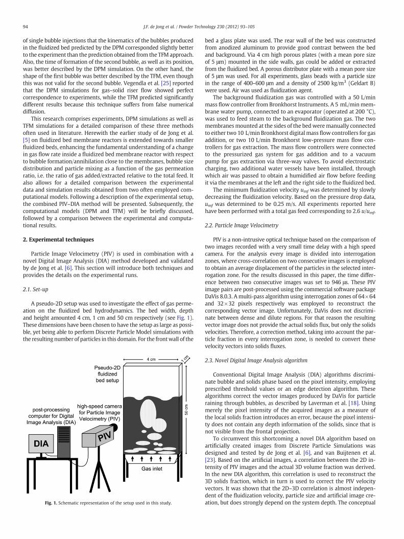
A pseudo-2D setup was used to investigate the effect of gas perme-ation on the fluidized bed hydrodynamics. The bed width, depthand height amounted 4 cm, 1 cm and 50 cm respectively (see Fig. 1).These dimensions have been chosen to have the setup as large as possi-ble, yet being able to perform Discrete Particle Model simulations withthe resulting number of particles in this domain. For the frontwall of the
Fig. 1. Schematic representation of the setup used in this study.
bed a glass plate was used. The rear wall of the bed was constructedfrom anodized aluminum to provide good contrast between the bedand background. Via 4 cm high porous plates (with a mean pore sizeof 5 μm) mounted in the side walls, gas could be added or extractedfrom the fluidized bed. A porous distributor plate with a mean pore sizeof 5 μm was used. For all experiments, glass beads with a particle sizein the range of 400–600 μm and a density of 2500 kg/m3 (Geldart B)were used. Air was used as fluidization agent.
The background fluidization gas was controlled with a 50 L/minmass flow controller from Bronkhorst Instruments. A 5 mL/minmem-brane water pump, connected to an evaporator (operated at 200 °C),was used to feed steam to the background fluidization gas. The twomembranesmounted at the sides of the bedweremanually connectedto either two 10 L/min Bronkhorst digitalmass flow controllers for gasaddition, or two 10 L/min Bronkhorst low-pressure mass flow con-trollers for gas extraction. The mass flow controllers were connectedto the pressurized gas system for gas addition and to a vacuumpump for gas extraction via three-way valves. To avoid electrostaticcharging, two additional water vessels have been installed, throughwhich air was passed to obtain a humidified air flow before feedingit via the membranes at the left and the right side to the fluidized bed.
The minimum fluidization velocity umf was determined by slowlydecreasing the fluidization velocity. Based on the pressure drop data,umf was determined to be 0.25 m/s. All experiments reported herehave been performed with a total gas feed corresponding to 2.6 u/umf.
2.2. Particle Image Velocimetry
PIV is a non-intrusive optical technique based on the comparison oftwo images recorded with a very small time delay with a high speedcamera. For the analysis every image is divided into interrogationzones, where cross-correlation on two consecutive images is employedto obtain an average displacement of the particles in the selected inter-rogation zone. For the results discussed in this paper, the time differ-ence between two consecutive images was set to 946 μs. These PIVimage pairs are post-processed using the commercial software packageDaVis 8.0.3. Amulti-pass algorithm using interrogation zones of 64×64and 32×32 pixels respectively was employed to reconstruct thecorresponding vector image. Unfortunately, DaVis does not discrimi-nate between dense and dilute regions. For that reason the resultingvector image does not provide the actual solids flux, but only the solidsvelocities. Therefore, a correction method, taking into account the par-ticle fraction in every interrogation zone, is needed to convert thesevelocity vectors into solids fluxes.
2.3. Novel Digital Image Analysis algorithm
Conventional Digital Image Analysis (DIA) algorithms discrimi-nate bubble and solids phase based on the pixel intensity, employingprescribed threshold values or an edge detection algorithm. Thesealgorithms correct the vector images produced by DaVis for particleraining through bubbles, as described by Laverman et al. [18]. Usingmerely the pixel intensity of the acquired images as a measure ofthe local solids fraction introduces an error, because the pixel intensi-ty does not contain any depth information of the solids, since that isnot visible from the frontal projection.
To circumvent this shortcoming a novel DIA algorithm based onartificially created images from Discrete Particle Simulations wasdesigned and tested by de Jong et al. [6], and van Buijtenen et al.[23]. Based on the artificial images, a correlation between the 2D in-tensity of PIV images and the actual 3D volume fraction was derived.In the new DIA algorithm, this correlation is used to reconstruct the3D solids fraction, which in turn is used to correct the PIV velocityvectors. It was shown that the 2D–3D correlation is almost indepen-dent of the fluidization velocity, particle size and artificial image cre-ation, but does strongly depend on the system depth. The conceptual
95J.F. de Jong et al. / Powder Technology 230 (2012) 93–105
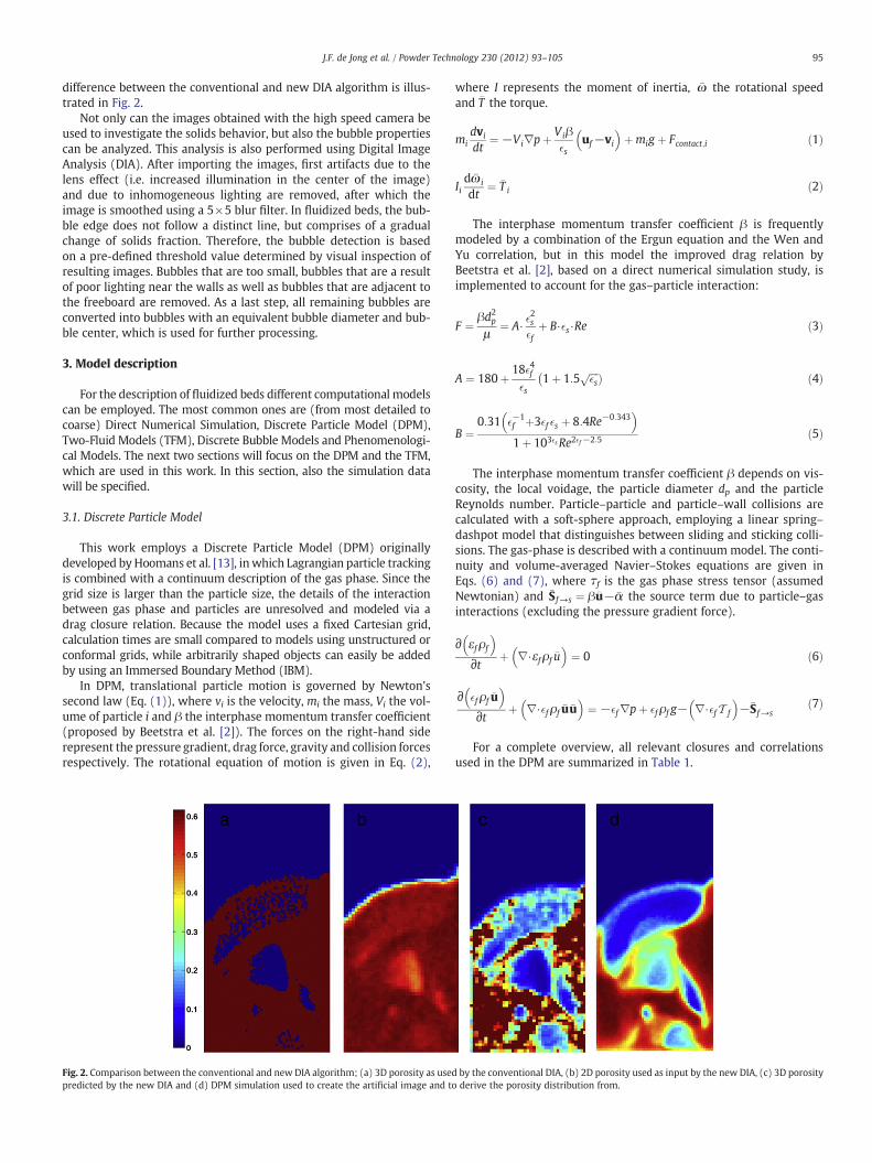
difference between the conventional and new DIA algorithm is illus-trated in Fig. 2.
Not only can the images obtained with the high speed camera beused to investigate the solids behavior, but also the bubble propertiescan be analyzed. This analysis is also performed using Digital ImageAnalysis (DIA). After importing the images, first artifacts due to thelens effect (i.e. increased illumination in the center of the image)and due to inhomogeneous lighting are removed, after which theimage is smoothed using a 5×5 blur filter. In fluidized beds, the bub-ble edge does not follow a distinct line, but comprises of a gradualchange of solids fraction. Therefore, the bubble detection is basedon a pre-defined threshold value determined by visual inspection ofresulting images. Bubbles that are too small, bubbles that are a resultof poor lighting near the walls as well as bubbles that are adjacent tothe freeboard are removed. As a last step, all remaining bubbles areconverted into bubbles with an equivalent bubble diameter and bub-ble center, which is used for further processing.
3. Model description
For the description of fluidized beds different computational modelscan be employed. The most common ones are (from most detailed tocoarse) Direct Numerical Simulation, Discrete Particle Model (DPM),Two-Fluid Models (TFM), Discrete Bubble Models and Phenomenologi-cal Models. The next two sections will focus on the DPM and the TFM,which are used in this work. In this section, also the simulation datawill be specified.
3.1. Discrete Particle Model
This work employs a Discrete Particle Model (DPM) originallydeveloped by Hoomans et al. [13], inwhich Lagrangian particle trackingis combined with a continuum description of the gas phase. Since thegrid size is larger than the particle size, the details of the interactionbetween gas phase and particles are unresolved and modeled via adrag closure relation. Because the model uses a fixed Cartesian grid,calculation times are small compared to models using unstructured orconformal grids, while arbitrarily shaped objects can easily be addedby using an Immersed Boundary Method (IBM).
In DPM, translational particle motion is governed by Newton'ssecond law (Eq. (1)), where vi is the velocity, mi the mass, Vi the vol-ume of particle i and β the interphase momentum transfer coefficient(proposed by Beetstra et al. [2]). The forces on the right-hand siderepresent the pressure gradient, drag force, gravity and collision forcesrespectively. The rotational equation of motion is given in Eq. (2),
Fig. 2. Comparison between the conventional and new DIA algorithm; (a) 3D porosity as usedpredicted by the new DIA and (d) DPM simulation used to create the artificial image and to
where I represents the moment of inertia, �ω the rotational speedand �T the torque.
midvidt
¼ −Vi∇pþ Viβ�s
uf−vi� �
þmig þ Fcontact;i ð1Þ
Iid �ω i
dt¼ �T i ð2Þ
The interphase momentum transfer coefficient β is frequentlymodeled by a combination of the Ergun equation and the Wen andYu correlation, but in this model the improved drag relation byBeetstra et al. [2], based on a direct numerical simulation study, isimplemented to account for the gas–particle interaction:
F ¼βd2pμ
¼ A⋅�2s
�fþ B⋅�s⋅Re ð3Þ
A ¼ 180þ18�4f�s
1þ 1:5ffiffiffiffi�s
p Þ�
ð4Þ
B ¼0:31 �
−1f þ3�f �s þ 8:4Re−0:343
� �1þ 103�s Re2�f−2:5 ð5Þ
The interphase momentum transfer coefficient β depends on vis-cosity, the local voidage, the particle diameter dp and the particleReynolds number. Particle–particle and particle–wall collisions arecalculated with a soft-sphere approach, employing a linear spring–dashpot model that distinguishes between sliding and sticking colli-sions. The gas-phase is described with a continuum model. The conti-nuity and volume-averaged Navier–Stokes equations are given inEqs. (6) and (7), where τf is the gas phase stress tensor (assumedNewtonian) and �S f→s ¼ β�u−�α the source term due to particle–gasinteractions (excluding the pressure gradient force).
∂ εfρf
� �∂t þ ∇⋅εfρf �u
� �¼ 0 ð6Þ
∂ �fρf �u� �
∂t þ ∇⋅�fρf �u�u� �
¼ −�f∇pþ �fρf g− ∇⋅�f T f
� �−�S f→s
ð7Þ
For a complete overview, all relevant closures and correlationsused in the DPM are summarized in Table 1.
by the conventional DIA, (b) 2D porosity used as input by the new DIA, (c) 3D porosityderive the porosity distribution from.
Rate of strain tensor D i; j ¼ 12 ∇�usð Þ þ ∇�usð ÞT� �
− 13∇⋅�usI
Partial slip boundarycondition [20]
I−nn� �
⋅εsTs⋅n ¼ αwallπεsρsg0ffiffiffiθ
p
2ffiffiffi3
pε0
us
εsqs⋅n ¼ −us⋅εsTs⋅n
þ
ffiffiffi3
pπ 1−e2n;wall
� �εsρsg0
ffiffiffiθ
p
4ε0θ
8>>>>>><>>>>>>:
Particle pressure ps=[1+2(1+en)εsg0]εsρsθ
Newtonian stress-tensor T s ¼ −μs ∇�u þ ∇�uð ÞT− 23�I ∇�uð Þ
h i
Bulk viscosity λs ¼ 43 εsρsdpg0 1þ enð Þ
ffiffiθπ
q
Shear viscosity μs ¼
1:01600596
πρsdp
ffiffiffiθπ
r
1þ 85
1þ enð Þ2
εsg0
�1þ 8
5εsg0
�
εsg0
þ 45εsρsdpg0 1þ enð Þ
ffiffiffiθπ
r
8>>>>>>>>><>>>>>>>>>:
Pseudo-Fourier fluctuating �qs ¼ −κs∇θkinetic energy flux
Pseudo-thermal conductivity κs ¼
1:0251375384
πρsdp
ffiffiffiθπ
r
1þ 125
1þ enð Þ2
εsg0
�1þ 12
5εsg0
�
εsg0
þ2εsρsdpg0 1þ enð Þffiffiffiθπ
r
8>>>>>>>>><>>>>>>>>>:
Dissipation of granular energy dueto inelastic particle–particlecollisions
γ ¼ 3 1−e2n� �
ε2s ρsg0θ 4dp
ffiffiθπ
q− ∇⋅�usð Þ
h i
96 J.F. de Jong et al. / Powder Technology 230 (2012) 93–105
3.2. Two-Fluid Model
In contrast to the DPM, the TFM does not longer distinguish singleparticles. Instead, a continuum description for the solids phase isemployed, resulting in a second set of conservation equations formass and momentum (similar to Eqs. (6) and (7), but then for thesolids phase):
∂ �sρsð Þ∂t þ∇⋅ �sρs�us
� �¼ 0 ð8Þ
∂ �sρs�us
� �∂t þ∇⋅ �sρs�us�us
� �¼ −�s∇pg−∇⋅�sT s−∇ps þ β �ug−�us
� �þ �sρs�g
ð9Þ
To describe the solids phase rheology, the widely used KineticTheory of Granular Flow (KTFG) is adopted: In this framework in ad-dition to the mass and momentum conservation equations the gran-ular temperature θ Eq. (10), accounting for frictional stresses due toparticle–particle and particle–wall collisions, needs to be solved.
23
∂ �sρsθð Þ∂t þ∇⋅ �sρsθ�us
� �� �¼ − ps
��I þ �sT s
� �: ∇�us −∇⋅ �s�qs
� �−3βθ−γ ð10Þ
In this equation, ��I is the unit tensor, �qs the pseudo-Fourier fluctu-ating kinetic energy flux and γ the dissipation rate of granular energydue to in-elastic particle–particle collisions. In the KTGF, collisions areassumed binary and quasi-instantaneous, and do not take long-termand multiple particle contact into account (which is the case in the
dense part of the fluidized bed). To correct for this shortcoming, thesolids phase viscosity μs and the solids phase pressure ps are split upinto a kinetic part and a frictional part, which are treated separately(after Johnson and Jackson [14] and Srivastava and Sundaresan [21]):
In these equations, F, r, s and Ψ are constants, ϕI represents theinternal angle of friction and ��Di; j the rate of strain tensor. An overviewof all closures is given in Table 2. For a detailed description of themodel the reader is referred to Laverman [17].
4. Experiments and simulations
In this study two different domains have been used. For DPM sim-ulations a minimum of six particle diameters in depth is required toavoid particle bridging between from and back walls. With respect
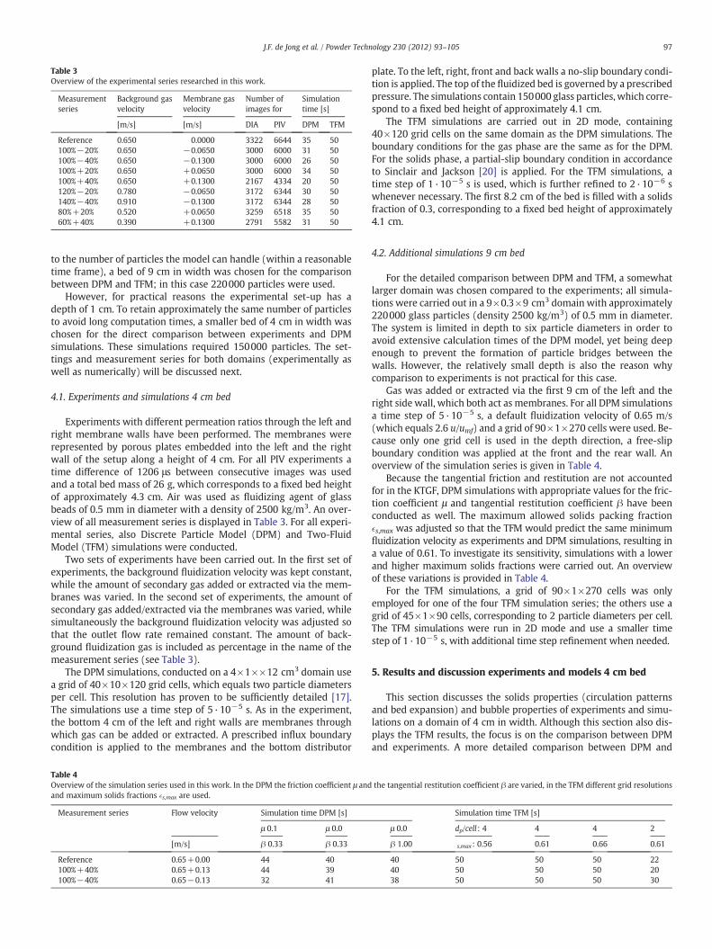
Table 3Overview of the experimental series researched in this work.
97J.F. de Jong et al. / Powder Technology 230 (2012) 93–105
to the number of particles the model can handle (within a reasonabletime frame), a bed of 9 cm in width was chosen for the comparisonbetween DPM and TFM; in this case 220000 particles were used.
However, for practical reasons the experimental set-up has adepth of 1 cm. To retain approximately the same number of particlesto avoid long computation times, a smaller bed of 4 cm in width waschosen for the direct comparison between experiments and DPMsimulations. These simulations required 150000 particles. The set-tings and measurement series for both domains (experimentally aswell as numerically) will be discussed next.
4.1. Experiments and simulations 4 cm bed
Experiments with different permeation ratios through the left andright membrane walls have been performed. The membranes wererepresented by porous plates embedded into the left and the rightwall of the setup along a height of 4 cm. For all PIV experiments atime difference of 1206 μs between consecutive images was usedand a total bed mass of 26 g, which corresponds to a fixed bed heightof approximately 4.3 cm. Air was used as fluidizing agent of glassbeads of 0.5 mm in diameter with a density of 2500 kg/m3. An over-view of all measurement series is displayed in Table 3. For all experi-mental series, also Discrete Particle Model (DPM) and Two-FluidModel (TFM) simulations were conducted.
Two sets of experiments have been carried out. In the first set ofexperiments, the background fluidization velocity was kept constant,while the amount of secondary gas added or extracted via the mem-branes was varied. In the second set of experiments, the amount ofsecondary gas added/extracted via the membranes was varied, whilesimultaneously the background fluidization velocity was adjusted sothat the outlet flow rate remained constant. The amount of back-ground fluidization gas is included as percentage in the name of themeasurement series (see Table 3).
The DPM simulations, conducted on a 4×1××12 cm3 domain usea grid of 40×10×120 grid cells, which equals two particle diametersper cell. This resolution has proven to be sufficiently detailed [17].The simulations use a time step of 5·10−5 s. As in the experiment,the bottom 4 cm of the left and right walls are membranes throughwhich gas can be added or extracted. A prescribed influx boundarycondition is applied to the membranes and the bottom distributor
Table 4Overview of the simulation series used in this work. In the DPM the friction coefficient μ andand maximum solids fractions �s,max are used.
Measurement series Flow velocity Simulation time DPM [s]
plate. To the left, right, front and back walls a no-slip boundary condi-tion is applied. The top of the fluidized bed is governed by a prescribedpressure. The simulations contain 150000 glass particles, which corre-spond to a fixed bed height of approximately 4.1 cm.
The TFM simulations are carried out in 2D mode, containing40×120 grid cells on the same domain as the DPM simulations. Theboundary conditions for the gas phase are the same as for the DPM.For the solids phase, a partial-slip boundary condition in accordanceto Sinclair and Jackson [20] is applied. For the TFM simulations, atime step of 1·10−5 s is used, which is further refined to 2·10−6 swhenever necessary. The first 8.2 cm of the bed is filled with a solidsfraction of 0.3, corresponding to a fixed bed height of approximately4.1 cm.
4.2. Additional simulations 9 cm bed
For the detailed comparison between DPM and TFM, a somewhatlarger domain was chosen compared to the experiments; all simula-tions were carried out in a 9×0.3×9 cm3 domain with approximately220000 glass particles (density 2500 kg/m3) of 0.5 mm in diameter.The system is limited in depth to six particle diameters in order toavoid extensive calculation times of the DPM model, yet being deepenough to prevent the formation of particle bridges between thewalls. However, the relatively small depth is also the reason whycomparison to experiments is not practical for this case.
Gas was added or extracted via the first 9 cm of the left and theright side wall, which both act as membranes. For all DPM simulationsa time step of 5·10−5 s, a default fluidization velocity of 0.65 m/s(which equals 2.6 u/umf) and a grid of 90×1×270 cells were used. Be-cause only one grid cell is used in the depth direction, a free-slipboundary condition was applied at the front and the rear wall. Anoverview of the simulation series is given in Table 4.
Because the tangential friction and restitution are not accountedfor in the KTGF, DPM simulations with appropriate values for the fric-tion coefficient μ and tangential restitution coefficient β have beenconducted as well. The maximum allowed solids packing fraction�s,max was adjusted so that the TFM would predict the same minimumfluidization velocity as experiments and DPM simulations, resulting ina value of 0.61. To investigate its sensitivity, simulations with a lowerand higher maximum solids fractions were carried out. An overviewof these variations is provided in Table 4.
For the TFM simulations, a grid of 90×1×270 cells was onlyemployed for one of the four TFM simulation series; the others use agrid of 45×1×90 cells, corresponding to 2 particle diameters per cell.The TFM simulations were run in 2D mode and use a smaller timestep of 1·10−5 s, with additional time step refinement when needed.
5. Results and discussion experiments and models 4 cm bed
This section discusses the solids properties (circulation patternsand bed expansion) and bubble properties of experiments and simu-lations on a domain of 4 cm in width. Although this section also dis-plays the TFM results, the focus is on the comparison between DPMand experiments. A more detailed comparison between DPM and
the tangential restitution coefficient β are varied, in the TFM different grid resolutions
Simulation time TFM [s]
μ 0.0 dp/cell : 4 4 4 2
β 1.00 s,max : 0.56 0.61 0.66 0.61
40 50 50 50 2240 50 50 50 2038 50 50 50 30
98 J.F. de Jong et al. / Powder Technology 230 (2012) 93–105
TFM will be given in Section 6 on a larger computational domain of9 cm in width.
5.1. Solids circulation patterns
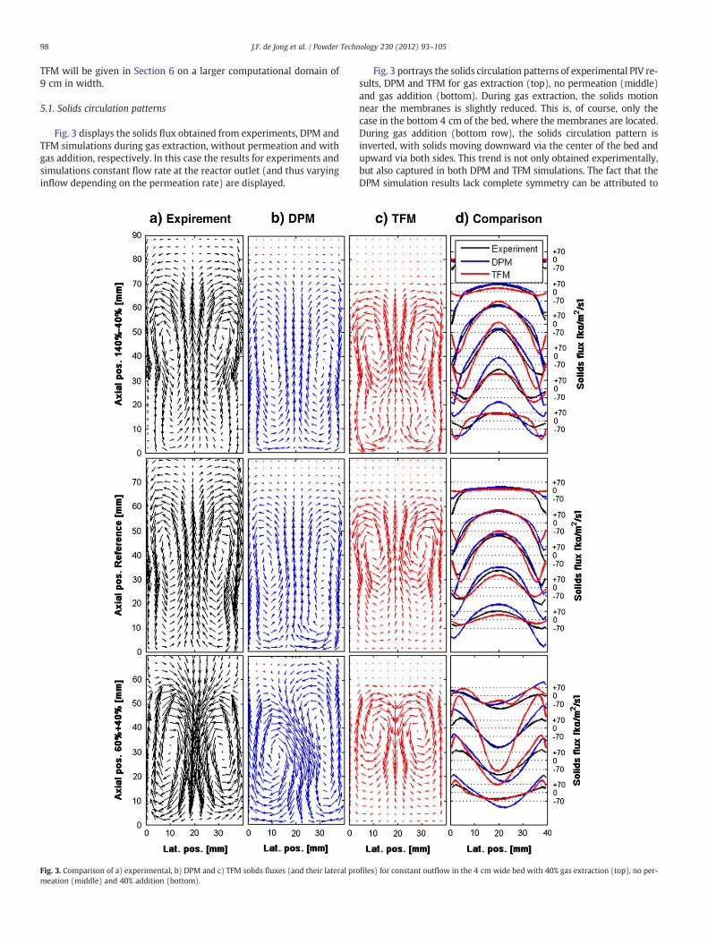
Fig. 3 displays the solids flux obtained from experiments, DPM andTFM simulations during gas extraction, without permeation and withgas addition, respectively. In this case the results for experiments andsimulations constant flow rate at the reactor outlet (and thus varyinginflow depending on the permeation rate) are displayed.
Fig. 3. Comparison of a) experimental, b) DPM and c) TFM solids fluxes (and their lateral promeation (middle) and 40% addition (bottom).
Fig. 3 portrays the solids circulation patterns of experimental PIV re-sults, DPM and TFM for gas extraction (top), no permeation (middle)and gas addition (bottom). During gas extraction, the solids motionnear the membranes is slightly reduced. This is, of course, only thecase in the bottom 4 cm of the bed, where the membranes are located.During gas addition (bottom row), the solids circulation pattern isinverted, with solids moving downward via the center of the bed andupward via both sides. This trend is not only obtained experimentally,but also captured in both DPM and TFM simulations. The fact that theDPM simulation results lack complete symmetry can be attributed to
files) for constant outflow in the 4 cm wide bed with 40% gas extraction (top), no per-
99J.F. de Jong et al. / Powder Technology 230 (2012) 93–105
the relatively short simulation time. Qualitatively, the solids circulationpatterns are in agreement with the trend as found experimentally in alarger fluidized bed of 30 cm in width [5]; for gas addition, the solidscirculation completely inverts, resulting in a solids upflow at the wallsand a solids downflow through the center of the bed.
Another noticeable difference between experiment, DPM simulationand TFM simulation is the bed expansion (see Fig 3). Although the ex-periment contains approximately 5% more particles (4.3 cm fixed bedheight versus 4.1 cm for the simulations), this cannot explain the differ-ence we observe in these graphs. In all three cases shown, the experi-mental bed expansion is clearly larger than the bed expansion for thenumerical cases. The TFM has the smallest bed expansion.
However, even in the graphs displaying the lateral profiles of theaxial solids fluxes, the direct comparison between the DPM and the
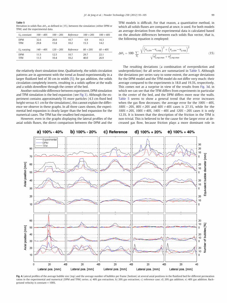
Fig. 4. Lateral profiles of the average bubble size (top) and the average number of bubbles peratios in the experimental and numerical (DPM and TFM) series. a) 40% gas extraction; b)ground velocity is constant=100%.
TFM models is difficult. For that reason, a quantitative method, inwhich all solids fluxes are compared at once, is used. For both modelsan average deviation from the experimental data is calculated basedon the absolute differences between each solids flux vector, that is,the following equation is employed:
The resulting deviations (a combination of overprediction andunderprediction) for all series are summarized in Table 5. Althoughthe deviations per series vary to some extent, the average deviationsfor the DPM model and the TFM model do not differ very much: theiraverage compared to the experiments is 18.0 and 19.3%, respectively.This comes not as a surprise in view of the results from Fig. 3d, inwhich we can see that the TFM differs from experiments in particularin the center of the bed, and the DPM differs more near the walls.Table 5 seems to show a general trend that the error increaseswhen the gas flow decreases; the average error for the 100%−40%,100%−20%, 80%+20% and 60%+40% cases is 27.1%, while for the100%+20%, 100%+40%, 140%−40% and 120%−20% cases it is only12.3%. It is known that the description of the friction in the TFM isnon-trivial. This is believed to be the cause for the larger error at de-creased gas flow, because friction plays a more dominant role in
r frame (bottom) at several axial positions in the fluidized bed for different permeation20% gas extraction; c) reference case; d) 20% gas addition; e) 40% gas addition. Back-
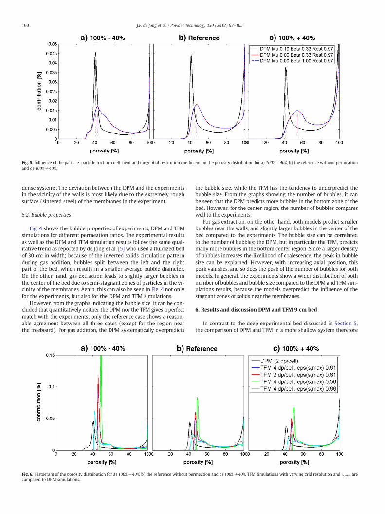
Fig. 5. Influence of the particle–particle friction coefficient and tangential restitution coefficient on the porosity distribution for a) 100%−40%, b) the reference without permeationand c) 100%+40%.
100 J.F. de Jong et al. / Powder Technology 230 (2012) 93–105
dense systems. The deviation between the DPM and the experimentsin the vicinity of the walls is most likely due to the extremely roughsurface (sintered steel) of the membranes in the experiment.
5.2. Bubble properties
Fig. 4 shows the bubble properties of experiments, DPM and TFMsimulations for different permeation ratios. The experimental resultsas well as the DPM and TFM simulation results follow the same qual-itative trend as reported by de Jong et al. [5] who used a fluidized bedof 30 cm in width; because of the inverted solids circulation patternduring gas addition, bubbles split between the left and the rightpart of the bed, which results in a smaller average bubble diameter.On the other hand, gas extraction leads to slightly larger bubbles inthe center of the bed due to semi-stagnant zones of particles in the vi-cinity of the membranes. Again, this can also be seen in Fig. 4 not onlyfor the experiments, but also for the DPM and TFM simulations.
However, from the graphs indicating the bubble size, it can be con-cluded that quantitatively neither the DPM nor the TFM gives a perfectmatch with the experiments; only the reference case shows a reason-able agreement between all three cases (except for the region nearthe freeboard). For gas addition, the DPM systematically overpredicts
Fig. 6. Histogram of the porosity distribution for a) 100%−40%, b) the reference without percompared to DPM simulations.
the bubble size, while the TFM has the tendency to underpredict thebubble size. From the graphs showing the number of bubbles, it canbe seen that the DPM predicts more bubbles in the bottom zone of thebed. However, for the center region, the number of bubbles compareswell to the experiments.
For gas extraction, on the other hand, both models predict smallerbubbles near the walls, and slightly larger bubbles in the center of thebed compared to the experiments. The bubble size can be correlatedto the number of bubbles; the DPM, but in particular the TFM, predictsmany more bubbles in the bottom center region. Since a larger densityof bubbles increases the likelihood of coalescence, the peak in bubblesize can be explained. However, with increasing axial position, thispeak vanishes, and so does the peak of the number of bubbles for bothmodels. In general, the experiments show a wider distribution of bothnumber of bubbles and bubble size compared to the DPM and TFM sim-ulations results, because the models overpredict the influence of thestagnant zones of solids near the membranes.
6. Results and discussion DPM and TFM 9 cm bed
In contrast to the deep experimental bed discussed in Section 5,the comparison of DPM and TFM in a more shallow system therefore
meation and c) 100%+40%. TFM simulations with varying grid resolution and �s,max are
101J.F. de Jong et al. / Powder Technology 230 (2012) 93–105
allows a larger domain width. For the discussion of the effect ofgas permeation on bed hydrodynamics we first focus on the solids cir-culation patterns, followed by the effect on the bubble properties.Subsequently, solids mixing will be discussed.
6.1. Solids circulation patterns
Figs. 5 and 6 compare the PDF's of the porosity of the simulationsobtained from the TFM model (with the DPM as reference) and theDPM simulations with and without particle–particle friction. It can
0
40
80
120
Axi
al p
osi
tio
n 1
00%
−40%
[m
m]
a/e/i)DPM Mu 0.1
b/f/j)DPM Mu 0.0
0
40
80
120
160
Axi
al p
osi
tio
n r
efer
ence
[m
m]
0 20 40 60 800
40
80
120
160
200
Lat. pos. [mm]
Axi
al p
osi
tio
n 1
00%
+40%
[m
m]
0 20 40 60 80Lat. pos. [mm]
0
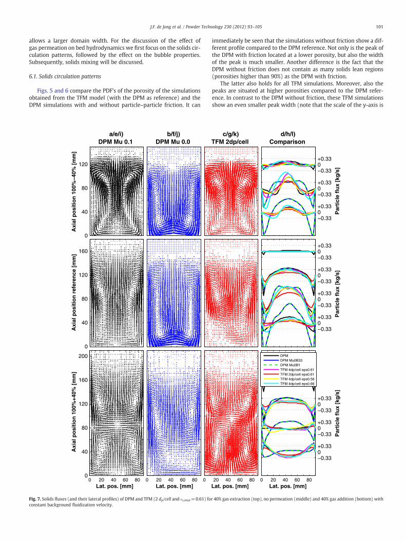
Fig. 7. Solids fluxes (and their lateral profiles) of DPM and TFM (2 dp/cell and �s,max=0.61) foconstant background fluidization velocity.
immediately be seen that the simulations without friction show a dif-ferent profile compared to the DPM reference. Not only is the peak ofthe DPM with friction located at a lower porosity, but also the widthof the peak is much smaller. Another difference is the fact that theDPM without friction does not contain as many solids lean regions(porosities higher than 90%) as the DPM with friction.
The latter also holds for all TFM simulations. Moreover, also thepeaks are situated at higher porosities compared to the DPM refer-ence. In contrast to the DPM without friction, these TFM simulationsshow an even smaller peak width (note that the scale of the y-axis is
102 J.F. de Jong et al. / Powder Technology 230 (2012) 93–105
different than in Fig. 5). It can be concluded that the TFM does not pro-duce the same distribution of porosity in the bed as the DPM. This dif-ference appears to be related to the treatment of friction in the TFM.
Fig. 7 shows the solids circulation pattern of the DPM, DPM with-out friction and the TFM. Note that for the DPM it does not matter ifthe tangential restitution coefficient β is set to 0.33 or to 1.00 (idealrestitution), which can be easily seen from the overlap of these twosimulations with respect to the lateral profiles (Fig. 7d/h/l). Also,out of the four TFM simulations (with varying grid resolution andmaximum solids packing fraction �s,max), only the solids circulationpattern of the high resolution cases is shown in Fig. 7; the solids cir-culation pattern of the other TFM simulations is similar and is onlyshown in the figure showing the comparison of the lateral profiles.
It can be concluded that the DPM simulation without friction (andwithout friction and ideal tangential restitution) completely fail to pre-dict the experimentally obtained solids circulation pattern: these simu-lations do not show stagnant zones during gas extraction (Fig. 7b),produce a much more pronounced solids circulation in the referencecase (Fig. 7f/h), and do not predict inversion of solids motion duringgas addition (Fig. 7j). These special DPM simulations were included inthis study to find out if the TFMwould coincide with these simulations.However, from these graphs it can evidently be concluded that there isno agreement between these DPM simulations and the TFM with re-spect to solids motion.
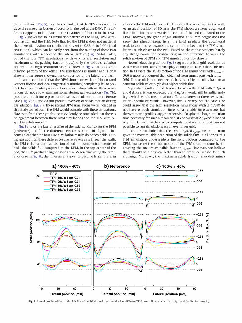
Fig. 8 shows the lateral profiles of the axial solids flux for the DPM(reference) and for the different TFM cases. From this figure it be-comes clear that the four TFM simulation results do not coincide. Dur-ing gas addition these differences are relatively small; near the walls,the TFM either underpredicts (top of bed) or overpredicts (center ofbed) the solids flux compared to the DPM. In the top center of thebed, the DPM predicts a higher solids flux. When examining the refer-ence case in Fig. 8b, the differences appear to become larger. Here, in
Fig. 8. Lateral profiles of the axial solids flux of the DPM simulation and the fo
all cases the TFM underpredicts the solids flux very close to the wall.At an axial position of 80 mm, the TFM shows a strong downwardflux a little bit more towards the center of the bed compared to theDPM. However, the graph of gas addition at 80 mm height does notshow this phenomenon: here, the DPM predicts the downwardpeak to exist more towards the center of the bed and the TFM simu-lations much closer to the wall. Based on these observations, hardlyany strong conclusion commenting on the difference between thesolids motion of DPM and TFM simulation can be drawn.
Nevertheless, the graphs of Fig. 8 suggest that both grid resolution aswell asmaximumsolids fraction play an important role in the solidsmo-tion. In all cases, the solids motion of the TFM simulations with �s,max=0.66 is more pronounced than obtained from simulations with �s,max=0.56. This result is not unexpected, because a higher solids fraction atconstant solids velocity yields a higher solids flux.
A peculiar result is the difference between the TFM with 2 dp/celland 4 dp/cell; it was expected that 4 dp/cell would still be sufficientlyhigh, which would mean that no difference between these two simu-lations should be visible. However, this is clearly not the case. Onecould argue that the high resolution simulations with 2 dp/cell donot have enough simulation time for a reliable time-average, butthe symmetric profiles suggest otherwise. Despite the long simulationtime necessary for such a resolution, it appears that 2 dp/cell is indeedrequired. Unfortunately, due to computational restrictions, it was notpossible to run simulations on an even finer grid.
It can be concluded that the TFM 2 dp/cell �s,max 0.61 simulationgives the most reliable prediction of the solids flux. In all series, thisTFM simulation underpredicts the solid motion compared to theDPM. Increasing the solids motion of the TFM could be done by in-creasing the maximum solids fraction �s,max. However, we believethere should be a physical rather than an empirical reason for sucha change. Moreover, the maximum solids fraction also determines
ur different TFM cases, all with constant background fluidization velocity.
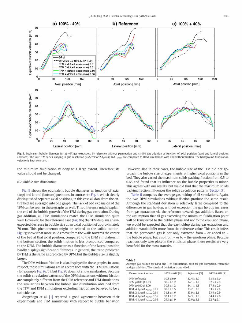
Fig. 9. Equivalent bubble diameter for a) 40% gas extraction, b) reference without permeation and c) 40% gas addition as function of axial position (top) and lateral position(bottom). The four TFM series, varying in grid resolution (4 dp/cell or 2 dp/cell) and �s,max, are compared to DPM simulations with and without friction. The background fluidizationvelocity is kept constant.
Table 6Average gas holdup for DPM and TFM simulations, both for gas extraction, referenceand gas addition. The standard deviation is provided.
Measurement series 100%−40% [%] Reference [%] 100%+40% [%]
103J.F. de Jong et al. / Powder Technology 230 (2012) 93–105
the minimum fluidization velocity to a large extent. Therefore, itsvalue should not be changed.
6.2. Bubble size distribution
Fig. 9 shows the equivalent bubble diameter as function of axial(top) and lateral (bottom) positions. In contrast to Fig. 4, which clearlydistinguished separate axial positions, in this case all data from the en-tire bed are averaged into one graph. The lack of bed expansion of theTFM can be seen in these graphs as well. This difference might explainthe end of the bubble growth of the TFM during gas extraction. Duringgas addition, all TFM simulations match the DPM simulation quitewell. However, for the reference case (Fig. 9b) the TFM displays an un-expected decrease in bubble size at an axial position of approximately70 mm. This phenomenon might be related to the solids motion;Fig. 7g shows thatmore solidsmove from thewalls towards the centerof the bed at that axial position, compared to the DPM simulation. Inthe bottom section, the solids motion is less pronounced comparedto the DPM. The bubble diameter as a function of the lateral positionhardly displays significant differences. In general, the trend predictedby TFM is the same as predicted by DPM, but the bubble size is slightlylarger.
The DPMwithout friction is also displayed in these graphs. In somerespect, these simulations are in accordancewith the TFM simulations(for example Fig. 9a/b), but Fig. 9c does not show similarities. Becausethe solids circulation patterns of the DPM simulations without frictionare completely different from the DPM reference and TFM simulations,the similarities between the bubble size distribution obtained fromthe TFM and DPM simulations excluding friction are believed to be acoincidence.
Asegehegn et al. [1] reported a good agreement between theirexperiments and TFM simulations with respect to bubble behavior.
However, also in their cases, the bubble size of the TFM did not ap-proach the bubble size of experiments at higher axial positions in thebed. They also varied the maximum solids packing fraction from 0.5 to0.65 and found that its influence on the bubble properties is minor.This agrees with our results, but we did find that the maximum solidspacking fraction influences the solids circulation pattern (Section 5).
Table 6 compares the average gas holdup of all simulations. Again,the two DPM simulations without friction produce the same result.Although the standard deviation is relatively large compared to thedifferences in gas holdup, without exception the gas holdup increasesfrom gas extraction via the reference towards gas addition. Based onthe assumption that all gas exceeding the minimum fluidization pointwill be transferred to the bubble phase and not to the emulsion phase,we would be expected that the gas-holdup during gas extraction andaddition would differ more from the reference value. This result infersthat the permeated gas is not only extracted from – or added to –
the bubble phase, but also from – or to – the emulsion phase. Becausereactions only take place in the emulsion phase, these results are verybeneficial for the mass transfer.
104 J.F. de Jong et al. / Powder Technology 230 (2012) 93–105
7. Conclusion
A pseudo-2D setup of 4 cm in width with flat membranes in theleft and right walls has been used to study the effect of gas extractionand gas addition on the solids circulation patterns and the bubbleproperties. The experimental results have been compared to simula-tion results obtained from DPM and TFM simulations. For a moredetailed comparison between these models, a slightly larger systemof 9 cm in width was chosen.
The experimental and computational results are in qualitativeagreement with earlier results obtained for a 30 cm wide bed withrespect to the inversion of the solids circulation and correspondingreduced bubble size during gas addition. However, both models alsoshow significant deviations from the experiment with respect tosolids motion and bubble size distribution. The TFM overpredictsthe solids flux in the upper part of the bed, while the DPM does soin the lower part and near the walls. In particular the TFM shows amuch smaller bed expansion compared to the experiments. The bubblesize distribution predicted by the TFM matches the experiment quitewell during gas addition (unlike the DPM, which predicts larger bub-bles), but fails during gas extraction (as does the DPM). A part of thisdiscrepancy can be explained by the lack of bed expansion. The PDF ofthe porosity predicted by DPM and TFM shows distinct differences;the emulsion in the DPM is significantly denser than the emulsion inthe TFM. Moreover, the TFM hardly contains solids lean regions. Tosome extent, this result from the TFM is similar to the porosity distribu-tion of a DPM simulation without particle friction. However, predictingthe solids circulation of the DPM simulation without particle frictioncompletely fails. The direct comparison between TFM and DPM in the9 cm bed also reveals that a coarser grid (with 4 dp/cell) is not sufficientfor the TFM and that variations of the maximum solids fraction areclearly visible in the resulting solids motion and bubble properties.
Although qualitative agreement was found, it can only be conclud-ed that both the DPM and the TFM show some serious shortcomingsand at this point in time cannot yet be used for quantitative predic-tions. Further research on the friction model of the TFM, in particularthe inclusion of tangential stresses into the KTGF, as well as a closerinvestigation of the use of boundary conditions might improve futuresimulations.
Symbols and abbreviations
Symbolsα part of drag force [ kg
m2s2]α specularity coefficient [−]B1, B2 constants [−]β interphase momentum transfer coefficient [ kg
m3s]β tangential restitution coefficient [−]C particle fluctuating velocity [m/s]��D rate of strain tensor [−]δ overlap [m]Dispn/t/fric normal/tangential/frictional energy dissipation [J]dp particle diameter [m]e restitution coefficient [−]Ekin/pot/rot kinetic/potential/rotational energy [J]� fluids/solids fraction [−]F force [N]F constant [−]g gravitational constant [ms2]γ dissipation of granular energy due to in-elastic particle–
particle collisions [ kgms3]��I unit vector [−]
I moment of inertia [kg m2]k spring stiffness [N/m]κ pseudo-thermal conductivity [kg/m/s]λ bulk viscosity [Pa s]
m mass [kg]μ (shear) viscosity [Pa s]μ friction coefficient [−]n normal unit vector [−]N number [−]η damping coefficient [Ns/m]ΦI internal angle of friction [rad]Φs solids flux [kgs ]Ψ constant [−]p pressure [Pa]qs pseudo-Fourier fluctuating kinetic energy flux [kgms]r position [m]r constant [−]R radius [m]ρ density [kgm3]s constant [−]Sdrag source term particle–fluid interaction [ kg
m2s2]t time [s]t tangential unit vector [−]T torque [Nm]τ stress tensor [Pa]θ granular temperature [m
Subscriptsa, b particle indicesc criticalexp experimentali particle indexf fluidg gas-phasekc kinetic and collisionalmf minimum fluidizationn normals solidsim simulationt tangential
AbbreviationsDIA Digital Image AnalysisDPM Discrete Particle ModelKTFG Kinetic Theory of Granular FlowPDF Probability Density FunctionPIV Particle Image VelocimetryTFM Two-Fluid Model
Acknowledgments
We gratefully acknowledge Agentschap NL, the agency for sustain-ability and innovation within the Dutch Ministry of Economic Affairs,for its financial support of this project (EOSLT06032).
References
[1] T.W. Asegehegn, M. Schreiber, H.J. Krautz, Numerical simulation and experimentalvalidation of bubble behavior in 2d gas–solid fluidized bedswith immersed horizon-tal tubes, Chemical Engineering Science 66 (21) (November 2011) 5410–5427.
[2] R. Beetstra, M.A. van der Hoef, J.A.M. Kuipers, Drag force of intermediate Reynoldsnumber flow past mono- and bidisperse arrays of spheres, AICHE Journal 53 (2)(February 2007) 489–501.
105J.F. de Jong et al. / Powder Technology 230 (2012) 93–105
[3] S. Benyahia, Validation study of two continuum granular frictional flow theories, In-dustrial and Engineering Chemistry Research 47 (22) (November 2008) 8926–8932.
[4] M. Chiesa, V. Mathiesen, J.A. Melheim, B. Halvorsen, Numerical simulation of par-ticulate flow by the Eulerian–Lagrangian and the Eulerian–Eulerian approachwith application to a fluidized bed, Computers and Chemical Engineering 29 (2)(January 2005) 291–304.
[5] J.F. de Jong, M. van Sint Annaland, J.A.M. Kuipers, Experimental study on the effects ofgas permeation throughflatmembranes on the hydrodynamics inmembrane-assistedfluidized beds, Chemical Engineering Science 66 (11) (June 2011) 2398–2408.
[6] J.F. de Jong, S.O. Odu, M. van Buijtenen, N.G. Deen, M. van Sint Annaland, J.A.M.Kuipers, Development and validation of a novel digital image analysis methodfor fluidized bed particle image velocimetry, Powder Technology 1 (1) (2012) 1.
[7] J. Ding, D. Gidaspow, A bubbling fluidization model using kinetic-theory of granularflow, AICHE Journal 36 (4) (April 1990) 523–538.
[8] L. Fries, S. Antonyuk, S. Heinrich, S. Palzer, DEM–CFD modeling of a fluidized bedspray granulator, Chemical Engineering Science 66 (11) (June 2011) 2340–2355.
[10] C. Hogue, D. Newland, Efficient computer-simulation of moving granular particles,Powder Technology 78 (1) (January 1994) 51–66.
[11] D. Hohner, S. Wirtz, H. Kruggel-Emden, V. Scherer, Comparison of the multi-sphere and polyhedral approach to simulate non-spherical particles within thediscrete element method: influence on temporal force evolution for multiple con-tacts, Powder Technology 208 (3) (April 2010) 643–656.
[12] B.P.B. Hoomans. Granular dynamics of gas–solid two-phase flows. PhD thesis,University of Twente, 1999.
[13] B.P.B. Hoomans, J.A.M. Kuipers, W.J. Briels, W.P.M. van Swaaij, Discrete particlesimulation of bubble and slug formation in a two-dimensional gas-fluidised bed:a hard-sphere approach, Chemical Engineering Science 51 (1) (January 1996)99–118.
[14] P.C. Johnson, R. Jackson, Frictional collisional constitutive relations for antigranulocytes-materials, with application to plane shearing, Journal of Fluid Mechanics 176(March 1987) 67–93.
[15] T. Kolkman. Personal, communication, 2012.[16] J.A.M. Kuipers, K.J. van Duin, F.P.H. van Beckum, W.P.M. van Swaaij, A
numerical-model of gas-fluidized beds, Chemical Engineering Science 47 (8)(June 1992) 1913–1924.
[17] J.A. Laverman. On the hydrodynamics in gas phase polymerization reactors. PhDthesis, Eindhoven University of Technology, 2010.
[18] J.A. Laverman, I. Roghair, M. van Sint Annaland, J.A.M. Kuipers, Investigation intothe hydrodynamics of gas–solid fluidized beds using particle image velocimetrycoupled with digital image analysis, Canadian Journal of Chemical Engineering86 (3) (June 2008) 523–535.
[19] J.J. Nieuwland, M. van Sint Annaland, J.A.M. Kuipers, Hydrodynamic modeling ofgas/particle flows in riser reactors, AICHE Journal 42 (6) (June 1996) 1569–1582.
[20] J.L. Sinclair, R. Jackson, Gas–particle flow in a vertical pipe with particle–particleinteractions, AICHE Journal 35 (9) (September 1989) 1473–1486.
[21] A. Srivastava, S. Sundaresan, Analysis of a fractional-kinetic model for gas–particleflow, Powder Technology 129 (1-3) (January 2003) 72–85.
[22] Y. Tsuji, T. Tanaka, T. Ishida, Lagrangian numerical-simulation of plug flow ofcohesionless particles in a horizontal pipe, Powder Technology 71 (3) (September1992) 239–250.
[23] M.S. van Buijtenen, M. Börner, N.G. Deen, S. Heinrich, S. Antonyuk, J.A.M. Kuipers,An experimental study on the effect of collision properties on spout fluidized beddynamics, Powder Technology 206 (1-2) (January 2011) 139–148.
[24] M.S. van Buijtenen, W.J. van Dijk, N.G. Deen, J.A.M. Kuipers, T. Leadbeater, D.J.Parker, Numerical and experimental study on multiple-spout fluidized beds,Chemical Engineering Science 66 (11) (June 2011) 2368–2376.
[25] S.N.P. Vegendla, G.J. Heynderickx, G.B. Marin, Comparison of Eulerian–Lagrangianand Eulerian–Eulerian method for dilute gas–solid flow with side inlet, Computersand Chemical Engineering 35 (7) (July 2011) 1192–1199.
[26] S. Vun, J. Naser, P. Witt, Extension of the kinetic theory of granular flow to includedense quasi-static stresses, Powder Technology 204 (1) (December 2010) 11–20.
[27] Z.Y. Zhou, A.B. Yu, P. Zulli, A new computationalmethod for studying heat transfer influid bed reactors, Powder Technology 197 (1–2) (January 2010) 102–110.