Comparison of Bayesian and Frequentist Meta-Analytical Approaches for Analyzing Time to Event Data By Brenda Crowe (Joint work with Monica Bennett, Karen Price, James Stamey and John Seaman Jr) Midwest Biopharmaceutical Statistics Workshop 2014
Transcript
Comparison of Bayesian and Frequentist Meta-Analytical
Approaches for Analyzing Time to Event Data
By Brenda Crowe
(Joint work with Monica Bennett, Karen Price, James Stamey and John Seaman Jr)
Meta-analysis (MA) refers to the combining of evidence from relevant studies using appropriate statistical methods to allow inferences to be made to the population of interest.
(Definition from FDA’s 2013 white paper on meta-analysis http://www.fda.gov/downloads/Drugs/NewsEvents/UCM372069.pdf)
• Lots of literature comparing MA methods for binary data
• E.g., Sweeting et al. (2004, 2006), Bradburn et al. (2007)
• Not much for time-to-event data, though anticipate problems similar to binary data
Background/Motivation
21 May 2014
6MBSW
• December 2008 FDA issued a guidance for assessing cardiovascular (CV) risk in diabetes drugs.
• The guidance requires that the upper limit of the 2-sided 95% confidence interval for the risk ratio be less than 1.8 prior to submission and less than 1.3 after submission.
• This can be shown by performing a meta-analysis of phase 2 and 3 clinical trials and if these are insufficient, a large safety trial must be conducted.
Background/Motivation
21 May 2014
7MBSW
• Used simulation study to compare the performance of several meta-analytic approaches in the survival analysis context.
• Considered two frequentist approaches and a Bayesian approach with and without informative prior.
Background/Motivation: Our Research
21 May 2014
Overview of statistical challenges and considerations for analysis of rare adverse events
21 May 2014 MBSW 8
Mostly for Binary Data
9MBSW
Statistical Issues with Meta-analysis of Rare/Sparse Adverse Event Data
• Standard inferences for meta-analysis rely on large sample approximations. They may not be accurate and reliable when number of events is low.
• Zero events observed in one or both treatment arms for some studies
• Low power to detect heterogeneity (especially when the number of studies is modest)
21 May 2014
10MBSW
Metrics and Methods
11MBSW
Metric Choices
Binary outcomes • risk difference (RD), • arcsin risk difference*• risk ratio (RR), • odds ratio (OR)
Time to event: hazard ratio, …
* The arcsin link is not often used in clinical trials, but it is the asymptotically variance-stabilizing transformation for the binomial distribution. This link is studied by, for example, Rücker et al. (2009).
21 May 2014
12MBSW
Behavior When Zero Events Occur in One or Both Arms of a Study
Difference Metrics• Risk difference is defined but its variance = 0 for total zero
studies• Arcsin difference and its variance are defined
Relative Metrics• Log odds ratio and log risk ratio are undefined (as are their
variances) • Hazard ratio and its variance are undefined
Note: methods for combining studies have different properties for handling zero events
method to estimate the among-study variance such as method of moments (DerSimonian Laird [DSL]), anova (Hedges and Olkin)
• Mixed effects logistic regression
Important: Stratify by study
21 May 2014 MBSW 13
*There are Bayesian versions of many of these methods. See, for example, Higgins and Spiegelhalter (2002). The paper includes some WinBugs code. See Deeks and Higgins (2010) for a concise overview of most of the non-Bayesian methods.
14MBSW
What do People do with Zero Cells
• Use a method that can handle zeros (e.g., MH risk difference, arcsin difference, Bayesian)
• Exclude studies with zero cells (more likely for relative metrics)
• Collapse ‘small’ studies with a similar randomization allocation ratio (Nissen, 2010)
• Use a continuity correction
21 May 2014
15MBSW
Continuity Corrections (3 Ways)
1. Constant• Add 0.5 (or some other fixed constant) to each cell
2. Treatment arm continuity correction• Choose a proportionality constant k• Add k / (Sample size for Opposite Treatment Arm) to
each cell• May be less biased in presence of severe imbalance
3. Empirical continuity correction• Based on an empirical estimate of the pooled effect
size using the non-zero event studies
Sweeting et al, Stat in Med, 2004 and 2006
21 May 2014
16MBSW
Which Method is Best?
It depends on . . .• Number of studies• Sample size per trial and arm• Event rate• Amount of heterogeneity
Note: None of the 2 major simulation studies (Bradburn et al., Sweeting et al.) assessed risk ratio.
21 May 2014
Comparison of Binary Methods (Excludes RR Methods) for Sparse Data• Alternative CCs perform better than the constant
• IV (OR and RD) and DSL (OR and RD) perform v. poorly
• Peto method performed well for very low event rates, but bias increases with greater group imbalance and larger treatment effect
• MH OR with no CC or alternative CC, logistic regression, exact stratified and Bayesian fixed effects perform fairly well (event rates >= 0.5% to 1% of the sample sizes studied in Sweeting and Bradburn)
• MH RD has low bias and low power for very sparse data
See Sweeting, 2004 & 2006 and Bradburn, 2007 for further info
Simulation Study
Meta-analytical approaches for analyzing time to event data
19MBSW
Overview of Methods
1. Standard Cox proportional hazards (CPH)
2. CPH with Firth correction term (penalized likelihood)
3. Bayesian CPH (with and without informative prior)
• All methods model two treatment arms and stratify by study
21 May 2014
20MBSW
Cox Proportional Hazards
• The proportional hazards survival model for patient i in study j is
• i = 1, … , ns
• j = 1, … , s• λ0j(t) is the baseline hazard for study j• xij = 1 if patient i in study j is on treatment and xij = 0
otherwise • β is the log hazard ratio.
)exp()(0 ijjij βxttH
21 May 2014
21MBSW
CPH with Firth Correction
• When events are rare the problem of monotone likelihood can be encountered. • Estimates may not be available due to lack of
convergence. • Estimates may be imprecise and have large standard
errors.
• Firth (1993) developed a penalization method used to reduce bias in maximum likelihood parameter estimates.
• Heinze and Schemper (2001) adapted the Firth method to be used with the Cox model.
21 May 2014
22MBSW
Bayesian CPH
• Basic model assumes constant baseline hazard over time and specifies prior distributions for λ and β.
2. More informative priors• Used shape parameter for gamma prior = 0.01, 0.02 and 0.05
for corresponding event rates• Rate parameter = 1• For log hazard ratio, for exp(beta) = 1.0, prior mean = 0• For exp(beta) = 1.3, prior mean was 0.25 and for exp(beta)=1.5,
prior mean was 0.5
Used prior variance of 2 for each. Informative priors were only used for first study grouping.
• For the Bayesian methods WinBUGS or OpenBUGS can be used.
• The models for the Bayesian methods are based on the model in the “Leuk: survival analysis using Cox regression” example in WinBUGS.
21 May 2014
Simulation Results
30MBSW
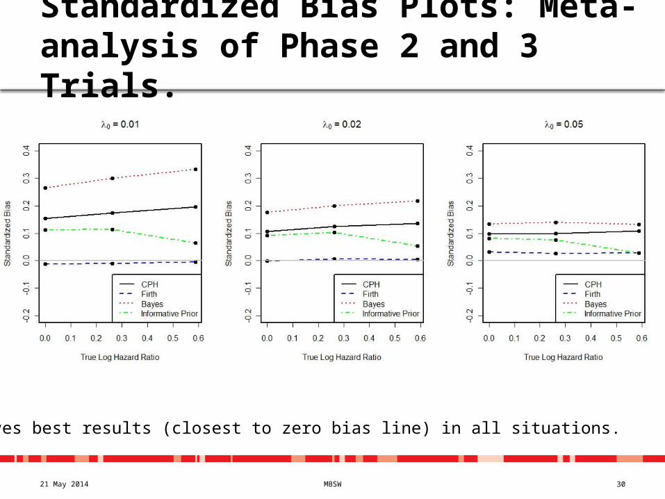
Standardized Bias Plots: Meta-analysis of Phase 2 and 3 Trials.
21 May 2014
Firth gives best results (closest to zero bias line) in all situations.
31MBSW21 May 2014
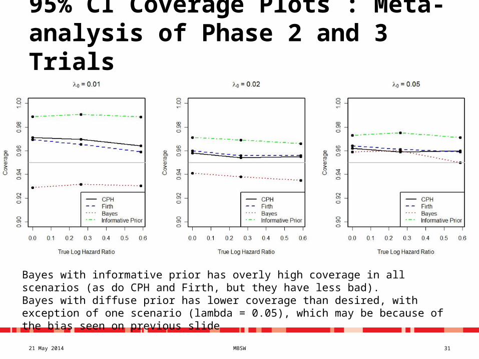
95% CI Coverage Plots : Meta-analysis of Phase 2 and 3 Trials
Bayes with informative prior has overly high coverage in all scenarios (as do CPH and Firth, but they have less bad).Bayes with diffuse prior has lower coverage than desired, with exception of one scenario (lambda = 0.05), which may be because of the bias seen on previous slide
32MBSW
Proportion of Upper Bounds Less Than 1.8: Meta-analysis of All Phase 2 and 3 Studies
21 May 2014
For true log HR = 0 and 0.262 (HR = 1, 1.3), higher proportions are better.For true HR = 1.8, lower are better.Firth does well/best in all situations.
33MBSW21 May 2014
Standardized Bias Plots : Meta-analysis of all Studies
All methods have std. bias close to zero, with exception of Bayesian method, where drops to -0.1for HR = 1.8.
34MBSW21 May 2014
95% CI Coverage Plots : Meta-analysis of all Studies
Coverage in most scenarios is between 0.94 and 0.96.Exceptions are when true log HR = 0. E.g., Bayes and CPH have coverage = 0.935 when baseline event rate is 0.01.
35MBSW
Proportion of Upper Bounds less than 1.8: Meta-analysis of All Studies.
21 May 2014
All methods perform well.
36MBSW
Concluding Remarks: Time to Event Data
• Based on the scenarios we studied, the Firth correction to the CPH is a good option for analyzing time-to-event data when the baseline event rate is low.
• For Bayesian method, informative prior reduces the bias of the estimated log HR.• However a misspecified prior makes the situation worse
(results not shown)• With larger number of events there is not a big difference
between the methods.
21 May 2014
37MBSW
Concluding Remarks: Binary Data
• IV and DSL poor choices for rare events• If need continuity correction, adding a constant to each
cell is not the best choice• Would Firth correction be good for binary data?
21 May 2014
38MBSW
References
21 May 2014
• Bender, R., Augustin, T., & Blettner, M. (2005). Generating survival times to simulate Cox proportional hazards models. Stat Med, 24(11), 1713-1723. doi: 10.1002/sim.2059
• Bennett, M. M., Crowe, B. J., Price, K. L., Stamey, J. D., & Seaman, J. W., Jr. (2013). Comparison of bayesian and frequentist meta-analytical approaches for analyzing time to event data. J Biopharm Stat, 23(1), 129-145. doi: 10.1080/10543406.2013.737210
• Berlin, J. A., & Colditz, G. A. (1999). The role of meta-analysis in the regulatory process for foods, drugs, and devices. JAMA, 281(9), 830-834.
• Berry, S. M., Berry, D. A., Natarajan, K., Lin, C.-S., Hennekens, C. H., & Belder, R. (2004). Bayesian survival analysis with nonproportional hazards: metanalysis of combination pravastatin–aspirin. Journal of the American Statistical Association, 99(465), 36-44.
• Bradburn, M. J., Deeks, J. J., Berlin, J. A., & Russell Localio, A. (2007). Much ado about nothing: a comparison of the performance of meta-analytical methods with rare events. Statistics in Medicine, 26(1), 53-77. doi: 10.1002/sim.2528
• Crowe, B. J., Xia, H. A., Berlin, J. A., Watson, D. J., Shi, H., Lin, S. L., . . . Hall, D. B. (2009). Recommendations for safety planning, data collection, evaluation and reporting during drug, biologic and vaccine development: a report of the safety planning, evaluation, and reporting team. Clin Trials, 6(5), 430-440. doi: 10.1177/1740774509344101
• Deeks, J. J., & Higgins, J. P. (2010). Statistical algorithms in Review Manager 5. http://tech.cochrane.org/revman/documentation/Statistical-methods-in-RevMan-5.pdf
• Firth, D. (1993). Bias reduction of maximum likelihood estimates. Biometrika, 80(1), 27-38.
• Heinze, G., & Ploner, M. (2002). SAS and SPLUS programs to perform Cox regression without convergence problems. Computer methods and programs in Biomedicine, 67(3), 217-223.
• Heinze, G., & Schemper, M. (2001). A solution to the problem of monotone likelihood in Cox regression. Biometrics, 57(1), 114-119.
• Higgins, J. P., & Spiegelhalter, D. J. (2002). Being sceptical about meta-analyses: a Bayesian perspective on magnesium trials in myocardial infarction. Int J Epidemiol, 31(1), 96-104.
• International Conference on Harmonisation (ICH). (1998). E9: Statistical Principles for Clinical Trials. International Conference on Harmonization Guidelines. http://www.ich.org/products/guidelines/efficacy/article/efficacy-guidelines.html
• Mantel, N., & Haenszel, W. (1959). Statistical aspects of the analysis of data from retrospective studies of disease. Journal of the National Cancer Institute, 22(4), 719-748.
• Nissen, S. E., & Wolski, K. (2010). Rosiglitazone revisited: an updated meta-analysis of risk for myocardial infarction and cardiovascular mortality. Archives of Internal Medicine, 170(14), 1191-1201. doi: 10.1001/archinternmed.2010.207
• O'Neill, R. T. (1988). Assessment of safety Biopharmaceutical Statistics for Drug Development: Marcel Dekker.• Proschan, M. A., Lan, K. K., & Wittes, J. T. (2006). Statistical Methods for Monitoring Clinical Trials. New York:
Springer.• Rucker, G., & Schumacher, M. (2008). Simpson's paradox visualized: the example of the rosiglitazone meta-
analysis. BMC Med Res Methodol, 8, 34. doi: 10.1186/1471-2288-8-34• Sutton, A. J., & Abrams, K. R. (2001). Bayesian methods in meta-analysis and evidence synthesis. Statistical
Methods in Medical Research, 10(4), 277-303. • Sutton, A. J., Cooper, N. J., Lambert, P. C., Jones, D. R., Abrams, K. R., & Sweeting, M. J. (2002). Meta-analysis
• Sweeting, M. J., Sutton, A. J., & Lambert, P. C. (2004). What to add to nothing? Use and avoidance of continuity corrections in meta-analysis of sparse data. Stat Med, 23(9), 1351-1375. doi: 10.1002/sim.1761
• Sweeting, M. J., Sutton, A. J., & Lambert, P. C. (2006). Correction. Statistics in Medicine, 25, 2700. • Tian, L., Cai, T., Pfeffer, M. A., Piankov, N., Cremieux, P.-Y., & Wei, L. (2009). Exact and efficient inference
procedure for meta-analysis and its application to the analysis of independent 2× 2 tables with all available data but without artificial continuity correction. Biostatistics, 10(2), 275-281.
• United States Food and Drug and Administration. (2008). Guidance for Industry: Diabetes Mellitus-Evaluating Cardiovascular Risk in New Antidiabetic Therapies to Treat Type 2 Diabetes. http://www.fda.gov/downloads/Drugs/GuidanceComplianceRegulatoryInformation/%20Guidances/UCM071627.pdf
• Warn, D., Thompson, S., & Spiegelhalter, D. (2002). Bayesian random effects meta‐analysis of trials with binary outcomes: methods for the absolute risk difference and relative risk scales. Statistics in Medicine, 21(11), 1601-1623.