1 COMPARISON OF BENDING PROFILES FOR ATOMIC FORCE MICROSCOPE CANTILEVERS TO FIXED-FREE EULER-BERNOULLI BEAM MODEL By LEE M. KUMANCHIK A THESIS PRESENTED TO THE GRADUATE SCHOOL OF THE UNIVERSITY OF FLORIDA IN PARTIAL FULFILLMENT OF THE REQUIREMENTS FOR THE DEGREE OF MASTER OF SCIENCE UNIVERSITY OF FLORIDA 2007
Transcript
1
COMPARISON OF BENDING PROFILES FOR ATOMIC FORCE MICROSCOPE CANTILEVERS TO FIXED-FREE EULER-BERNOULLI BEAM MODEL
By
LEE M. KUMANCHIK
A THESIS PRESENTED TO THE GRADUATE SCHOOL OF THE UNIVERSITY OF FLORIDA IN PARTIAL FULFILLMENT
OF THE REQUIREMENTS FOR THE DEGREE OF MASTER OF SCIENCE
Cantilever against a Rigid Surface .........................................................................................30 Cantilever against Cantilever ..................................................................................................32
5 DATA ANALYSIS ................................................................................................................39
4-1 Designations for each cantilever tested ...................................................................................37
4-2 Cantilever experimental combinations, 27 in total ..................................................................38
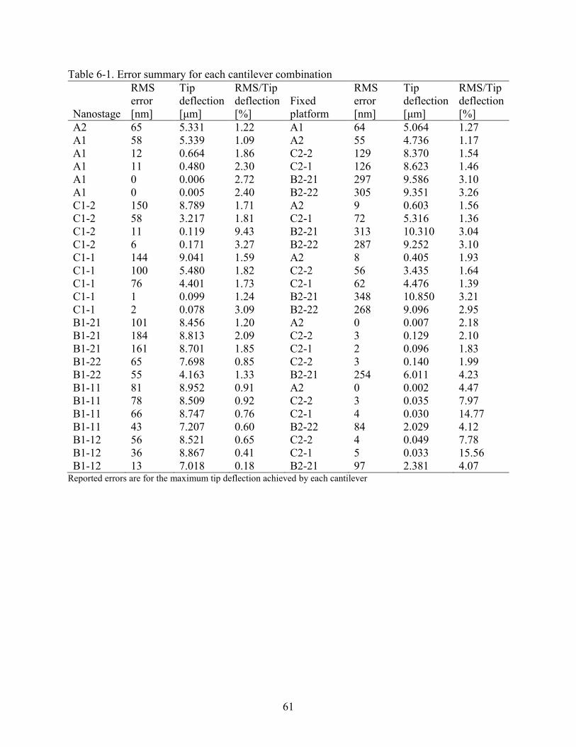
6-1 Error summary for each cantilever combination .....................................................................61
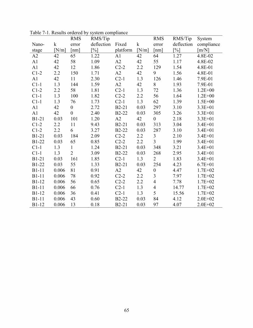
7-1 Results ordered by system compliance ....................................................................................65
7-2 Data for cantilever against a rigid surface ...............................................................................66
7
LIST OF FIGURES
Figure page 3-1 Computer generated image of the experimental setup. ...........................................................22
3-2 Schematic of SWLI operation. ................................................................................................23
3-3 Example scan of the smooth silicon surface. The 6 um difference from lowest to highest point is a result of contamination on the surface, possibly dust. .............................................24
3-4 Example cantilever placement on the aluminum holders. Individual cantilevers are too small to see but the monolithic base chips are labeled (A1-C2). If the holders were unscrewed and rotated in the indicated direction, the next experiment would be C1 against C2.................................................................................................................................25
3-5 The silicon holder nests against the machined feature in the aluminum holder. The cantilever A is nested against the micromachined slot in the silicon holder. Artifact B rests in a similar position. Though the cantilever and artifact aren’t visible, their
monolithic base chips are labeled (A,B). .................................................................................26
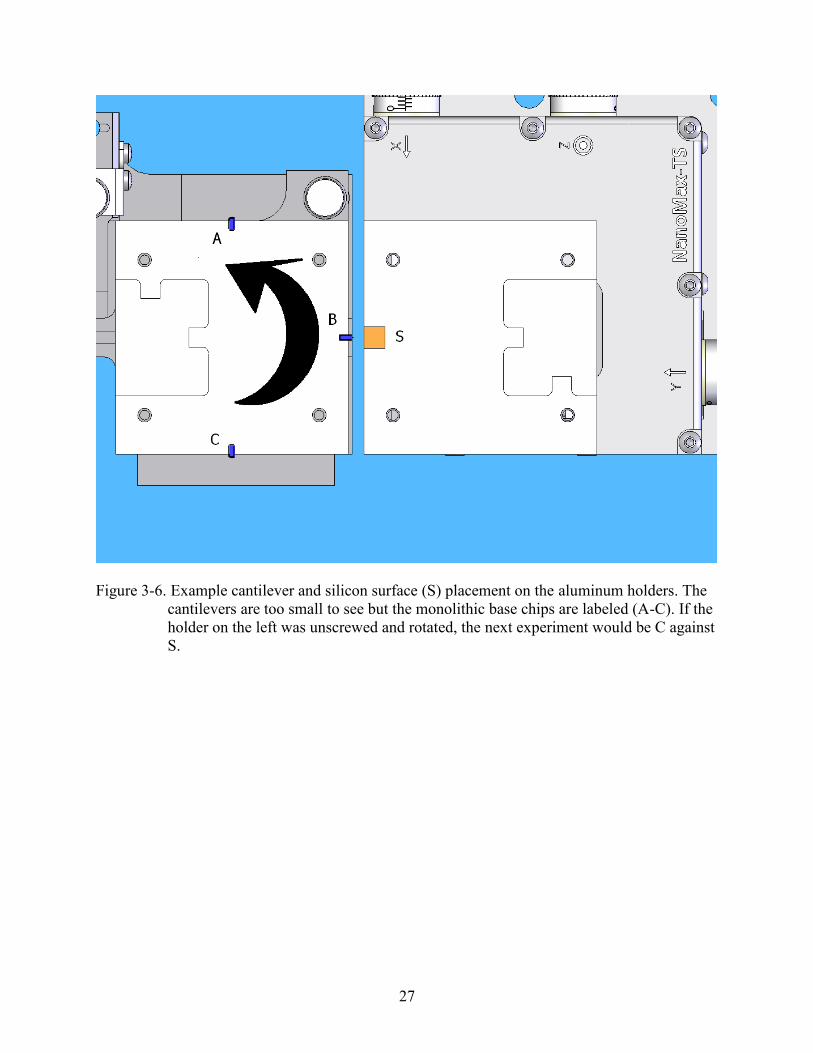
3-6 Example cantilever and silicon surface (S) placement on the aluminum holders. The cantilevers are too small to see but the monolithic base chips are labeled (A-C). If the holder on the left was unscrewed and rotated, the next experiment would be C against S. ....27
3-6 Complete setup of stages on the adapter plate connected to the SWLI motorized stage located under the SWLI objective............................................................................................29
4-1 Schematic of each cantilever used in the experiments with their designations. ......................34
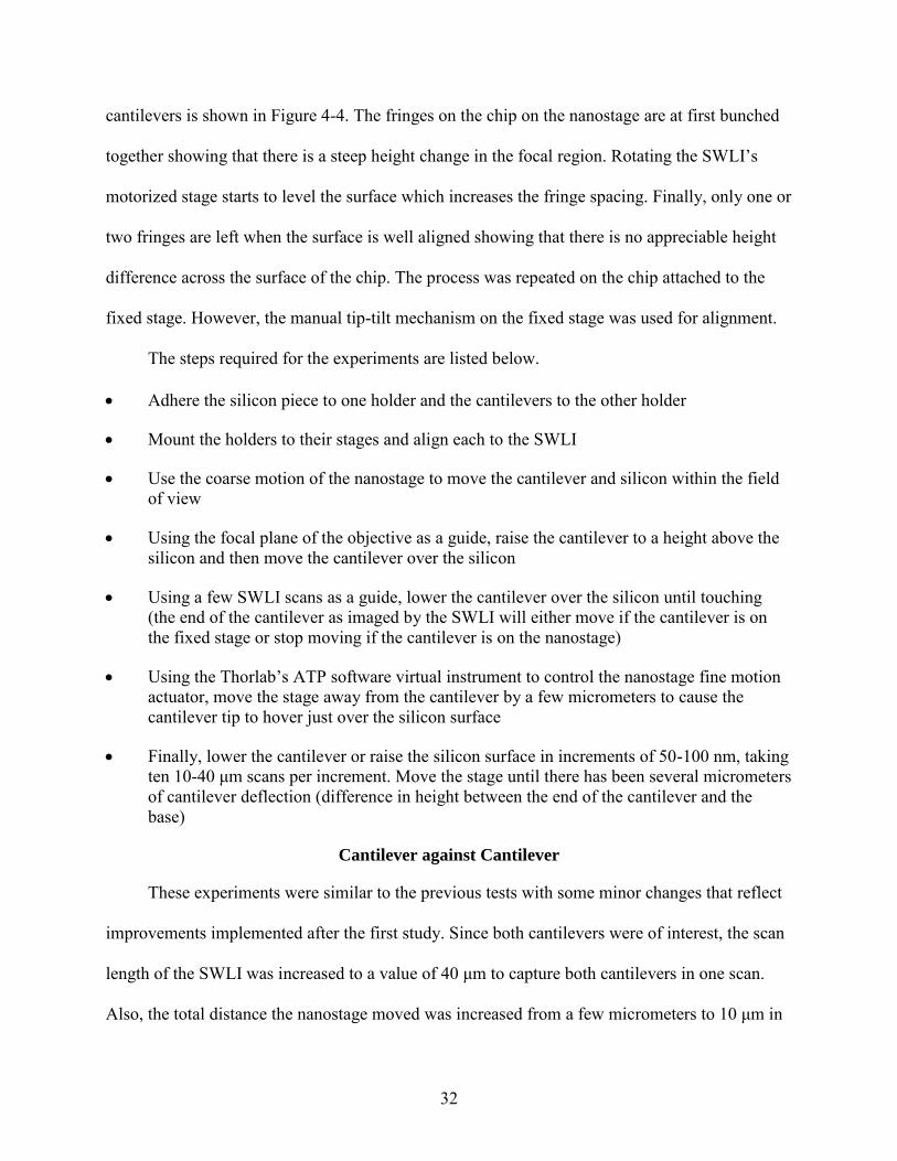
4-2 Schematic of the first cantilever for the first experiment ........................................................35
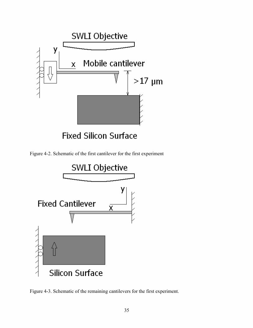
4-3 Schematic of the remaining cantilevers for the first experiment. ............................................35
4-4 Aligning the cantilevers with the SWLI objective. Align the cantilever on the nanostage (1-3) and then the cantilever on the fixed stage (4-6). When only one or two interference fringes can be seen the cantilevers are aligned (3 and 6). ........................................................36
4-5 Schematic of the second experiment. ......................................................................................36
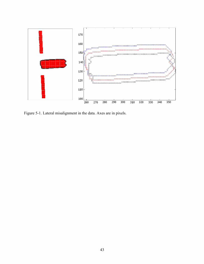
5-1 Lateral misalignment in the data. Axes are in pixels. ..............................................................43
5-2 Example view of cantilever in contact with a silicon surface (1), the SWLI surface map (2), and the cross-section used for data analysis (3). ...............................................................44
5-3 The cantilever on the left has a base that merges with a larger piece at (1), while the cantilever on the right has its base located at the last point before data dropout (2). ..............44
8
5-4 The base line defines the starting point of the cantilever and is calculated by a line fit to the flange edges. The section line defines the location of the 2D section for comparison to the bending equation. The thick line on top of the section line is the data belonging to the left cantilever. A new section line is calculated for the right cantilever. ...........................45
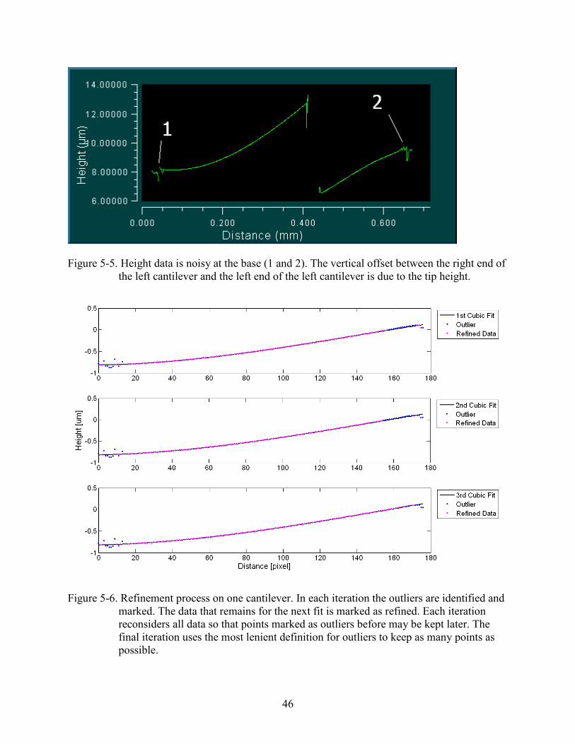
5-5 Height data is noisy at the base (1 and 2). The vertical offset between the right end of the left cantilever and the left end of the left cantilever is due to the tip height. ...........................46
5-6 Refinement process on one cantilever. In each iteration the outliers are identified and marked. The data that remains for the next fit is marked as refined. Each iteration reconsiders all data so that points marked as outliers before may be kept later. The final iteration uses the most lenient definition for outliers to keep as many points as possible. .....46
6-1 Cantilever C1 pressed against the silicon surface. RMS error is linearly dependent on tip deflection..................................................................................................................................52
6-2 Cantilever B against the silicon surface. RMS error has no clear relationship to tip deflection and the curve fit is very different from the actual data. Cantilever damage at the base was inferred. ...............................................................................................................52
6-3 Cantilever A1 from test A1 on A2. The RMS error is linearly dependent on tip deflection..................................................................................................................................53
6-4 Cantilever A1 from test A2 on A1. The RMS error is again linearly dependent on tip deflection. No hinge behavior as with the previous cantilever against rigid surface test for the same stage configuration. .............................................................................................53
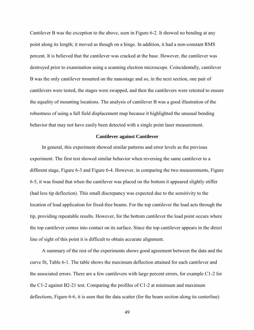
6-5 Comparison of the same cantilever when in the top position (pusher) versus the bottom position (pushee). The bottom position makes the cantilever appear stiffer. ..........................54
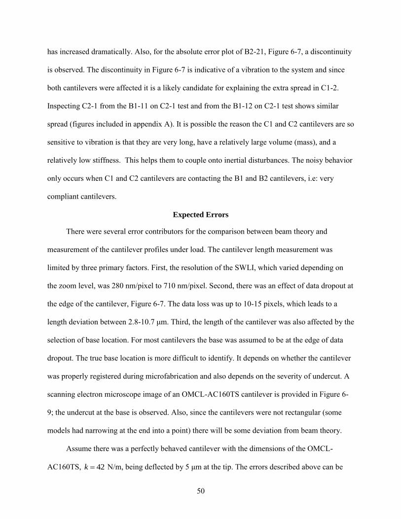
6-6 Cantilever C1-2 shows a sudden increase in data spread from tip position (1) to (2). ............54
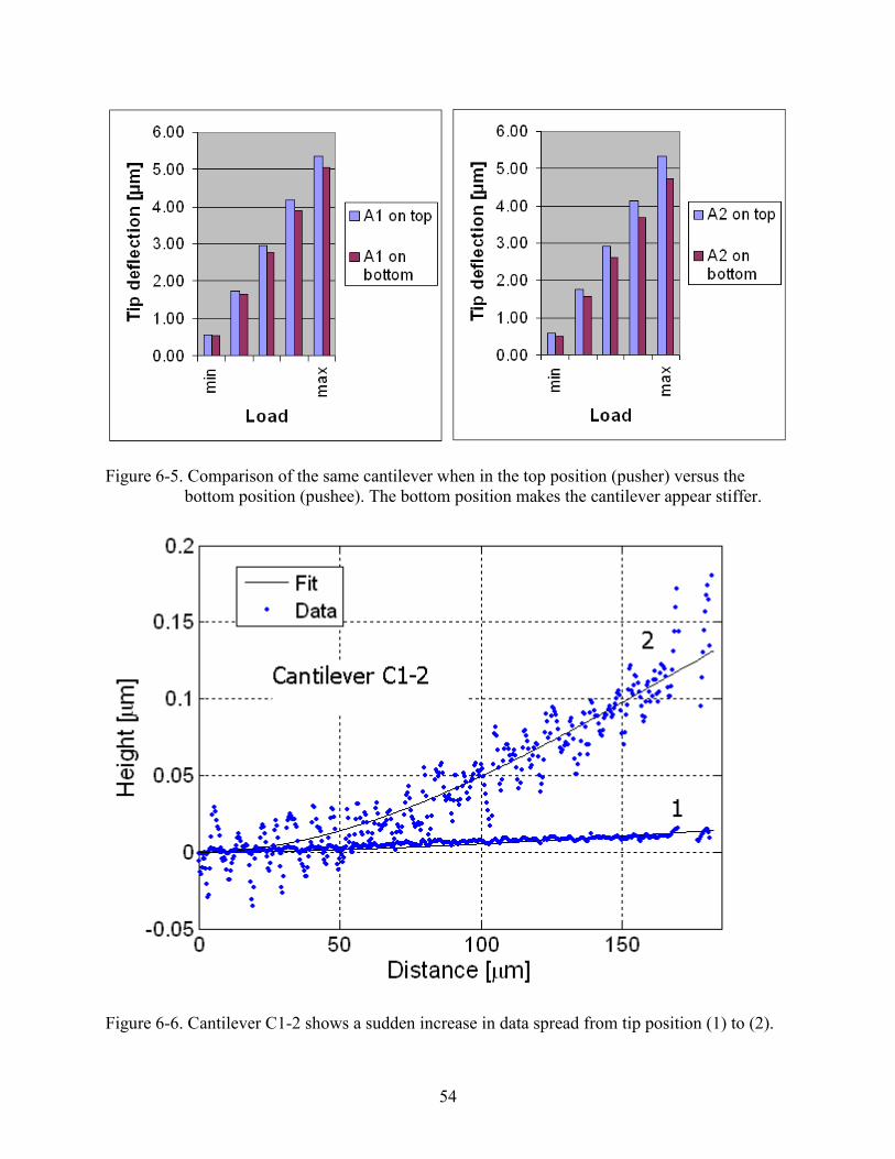
6-7 Absolute value of error for cantilever B2-21 during the C1-2 on B2-21 test. The discontinuity at (1) suggests the cantilevers experienced a vibration. .....................................55
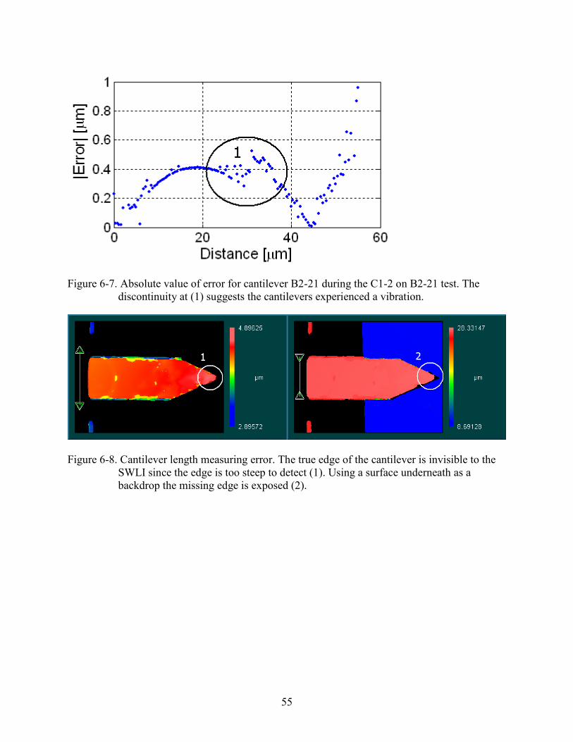
6-8 Cantilever length measuring error. The true edge of the cantilever is invisible to the SWLI since the edge is too steep to detect (1). Using a surface underneath as a backdrop the missing edge is exposed (2). ..............................................................................................55
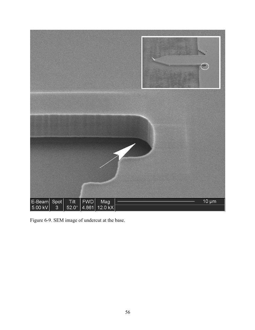
6-9 SEM image of undercut at the base. ........................................................................................56
6-10 Error curve if a perfect OMCL-AC160TS had a length error of 10 μm. RMS error is 7
6-11 Cantilever with profile data set to the depicted coordinate system. Actual coordinate system should be 10 μm further back. ..................................................................................58
9
6-12 Error curve if a perfect OMCL-AC160TS had an error locating the base by 10 μm.
RMS error is 89 nm..................................................................................................................59
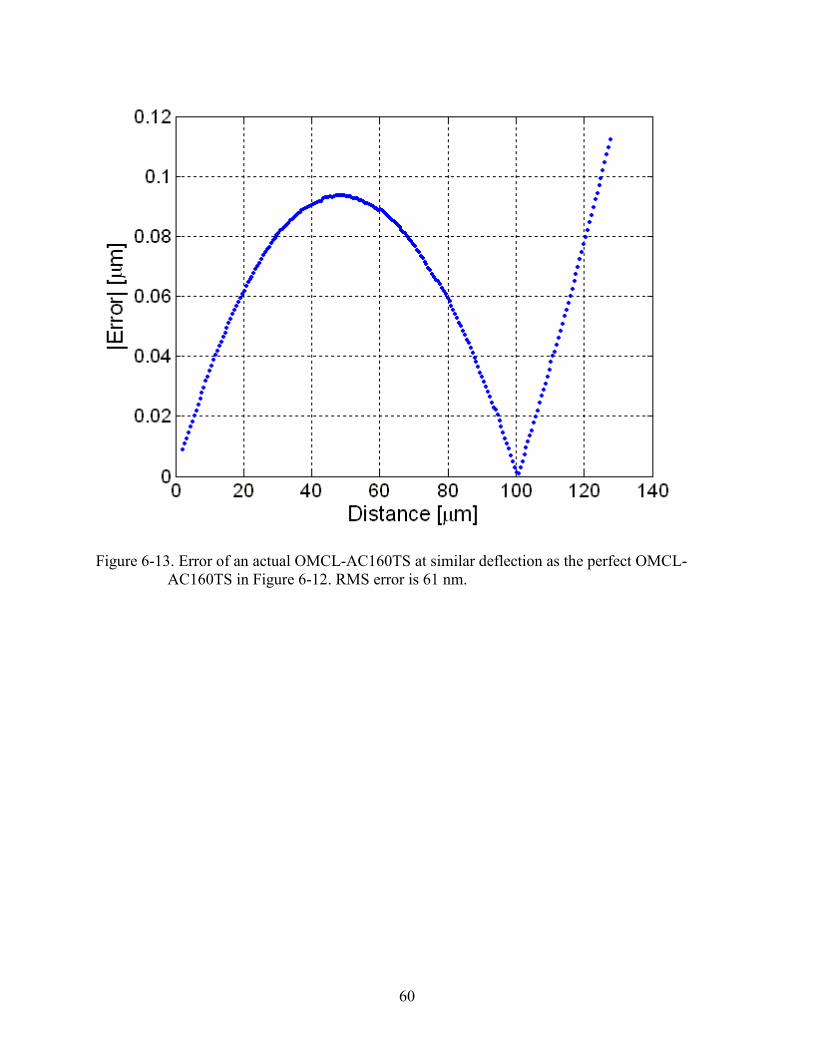
6-13 Error of an actual OMCL-AC160TS at similar deflection as the perfect OMCL-AC160TS in Figure 6-12. RMS error is 61 nm. ......................................................................60
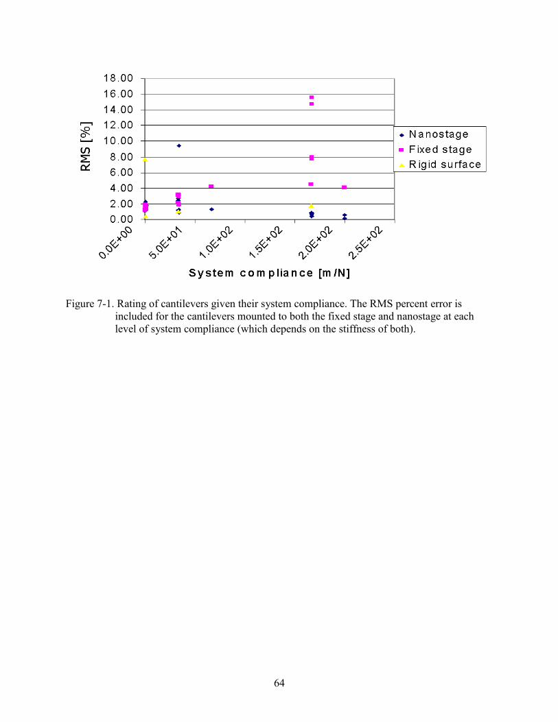
7-1 Rating of cantilevers given their system compliance. The RMS percent error is included for the cantilevers mounted to both the fixed stage and nanostage at each level of system compliance (which depends on the stiffness of both). .............................................................64
A-1 Cantilever C2 against the silicon surface. RMS error is linearly dependent on tip deflection..................................................................................................................................67
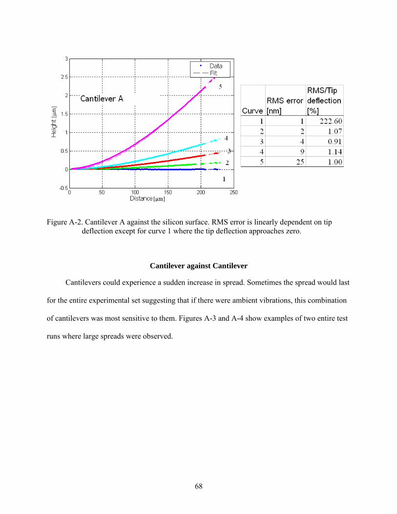
A-2 Cantilever A against the silicon surface. RMS error is linearly dependent on tip deflection except for curve 1 where the tip deflection approaches zero. .................................68
A-3 Cantilever C2-1 from B1-11 against C2-1. Significant spread in the data is observed. .........69
A-4 Cantilever C2-1 from B1-12 against C2-1. Significant spread in the data is observed. .........69
10
Abstract of Thesis Presented to the Graduate School of the University of Florida in Partial Fulfillment of the
Requirements for the Degree of Master of Science
COMPARISON OF BENDING PROFILES FOR ATOMIC FORCE MICROSCOPE CANTILEVERS TO FIXED-FREE EULER- BERNOULLI BEAM MODEL
By
Lee M. Kumanchik
August 2007
Chair: Tony L. Schmitz Major: Mechanical Engineering
The widespread use of atomic force microscopy as a fundamental metrology tool for
measuring forces in the nano- to micro-Newton range emphasizes the need for traceable
calibration of the force sensor. Currently, efforts are being made at national measuring institutes
to create calibration artifacts for the eventual dissemination of the unit of force. These will be
load bearing devices that will require intimate surface contact with atomic force microscope
cantilever tips to operate. Since these cantilever tips are sharpened to near atomic precision their
interactions with the surface are governed by microscale physics which are heavily influenced by
friction, van der Waals forces, and fluid film layers. The goal of our project was to study the
bending profiles of real atomic force microscope cantilevers to see if they behaved as fixed-free
beams. If the surface forces were strong enough to bind the tip during loading, the cantilever
would no longer act as a fixed-free beam and this could be observed. An assembly was fabricated for measuring the entire full field displacement of the
cantilever during static loading. This assembly mainly consisted of a three-dimensional optical
profiler for measuring cantilever bending shape and a three-axis parallel kinematics
nanopositioning stage for manipulating the cantilevers. Two types of experiments were
performed. One was for cantilevers contacting a rigid surface. The other was for cantilevers
11
contacting compliant surfaces. Each cantilever was rated based on how well its profile matched
up to the Euler-Bernoulli beam equation for a fixed-free beam. Poor fits indicated possible
deviant tip behavior and merited further investigation.
In general it was found that cantilevers fit well to the beam equation. Deviation from
theory did increase for greater loads at a linear rate with respect to tip displacement. The
experimental setup was robust enough to detect an anomalous cantilever. This cantilever did not
develop curvature under loading; it bent as though on a hinge and may have been cracked at the
base. It did not survive further tests. It was determined that the most sensitive parameter to error
was the location of the base. This location had to be inferred and remains an area to improve for
future work. Significant deviations to the beam equation were not observed.
12
CHAPTER 1 INTRODUCTION
The atomic force microscope (AFM) is unique in its ability to measure many different
properties using one mechanical sensor. This flexibility has allowed the instrument to find use in
multiple disciplines, such as biology, metrology, chemistry, fluid mechanics, tribology, and
material science. Further, it is currently the instrument of choice for measuring forces in the
nano- to micro-Newton range. It is for this reason that calibration of the force sensor is of
fundamental importance. The force sensor is a cantilever beam that is idealized as a linear spring
following Hooke’s law F kx , where F is applied force, x is the resulting displacement, and
k is the spring constant of the system.
The use of the AFM in small force metrology is therefore limited to the accuracy with
which k is known. Proper calibration of k should follow a clear path of traceability to the
Système International d’Unités (SI). Traceability is the chain of calibrations that link each
sensor/instrument through a direct path, with defensible uncertainty statements for each
measurement, to a primary standard. This primary standard, which reflects a physical realization
of the unit of measure, is defined and maintained (if necessary) by national measurement
institutes (NMIs). Traceability enables measurement uncertainty to propagate through the chain
of calibrations and thus identifies the uncertainty for measurements performed by a given sensor
or instrument. This notion of standardized units and measures allows quantitative data to be
compared between organizations/manufacturers/laboratories, facilitating collaboration and
reproducibility of results.
There have been many efforts to calibrate the AFM force sensor, dating back nearly two
decades, (see Table 1-1 for a summary, see Chapter 2 for details), but only in the past few years
has the focus shifted to traceability to a primary standard. The widespread adoption of the AFM
13
has motivated the NMIs to develop a force realization for the nano- to micro-Newton force
regime. In particular, the National Institute of Standards and Technology (NIST), Gaithersburg,
MD, has developed a force realization based on electrical units. As part of this effort,
collaboration between the University of Florida (UF), Gainesville, FL, and NIST has fostered a
project to develop a reference standard for AFM for the eventual dissemination of the unit of
force.
Table 1-1. Summary of different calibration techniques Type of calibration Author Geometric model of V-shaped beam Gibson et al. [1] Geometric model of trapezoidal cross-section Poggi et al. [2] Biological force artifact Blank et al. [3] Resonant frequency + added mass Cleveland et al. [4] Resonant frequency + Q factor in fluid (air) Sader et al. [5] Resonant frequency + thin gold layer Gibson et al. [6] Resonant frequency + pre-calibrated cantilever on the same chip Gibson et al. [7] Resonant frequency + inkjet water droplet Golovko et al. [8] Resonate colloidal tip in a confined fluid + measure dynamic response Notley et al. [9] Thermal noise spectrum Butt et al. [10] Microfabricated array of reference springs (MARS) Cumpson et al. [11] Torsional MARS Cumpson et al. [12] Cantilever MARS (C-MARS) Cumpson et al. [13] Macrolever Torii et al. [14] Electrostatic force balance Newell et al. [15] Pre-calibrated piezolever Pratt et al. [16] Repeatability of manufactured cantilevers Gates et al. [17] Nanoindentation apparatus Holbery et al. [18] Microfabricated electrical nanobalance Cumpson et al. [19]
The end goal of this UF-NIST project is the production of flexure-based artifacts that
exhibit low fabrication expense, stiffness adjustability by design, insensitivity to load application
point, mechanical robustness, and good reproducibility. Once an artifact is calibrated at NIST it
can be used to calibrate AFM cantilevers. This process would consist of forcing the cantilever’s
tip against the loading surface of the artifact and measuring the artifact and tip displacements,
i.e., the measurand is displacement, which can be determined using the AFM metrology. When
14
compared to other calibration methods that require the measurement of multiple geometric
dimensions, or material properties, or temperature, to infer stiffness, the benefit is clear.
The drawback to using artifacts is that the calibration process involves direct surface
contact with the AFM cantilever tip. It could be argued that this better reflects the measurement
environment but there are types of tips, such as those used for biological samples, which can
only contact a surface once. It is of interest, however, to include the surface interactions that are
usually neglected in the macroscale world. The microscopic AFM tip is exposed to an exotic
world of physics where van der Waals forces are strong, fluid films create powerful capillary
forces, and electrical charges can manifest in electrically neutral materials. These forces have
been posited as confounding calibration of ultra-compliant AFM cantilevers.
The goal of this project is to determine if the assumed fixed-free beam model is adequate,
given the complicated tip force conditions. It is typically assumed that the cantilever tip is free to
slide and rotate so that the AFM cantilever is can be modeled as a fixed-free beam of rectangular
cross-section. The interaction with translational binding forces at the base, such as friction, could
invalidate the free boundary condition. Likewise, any force that binds the tip from rotation would
also invalidate the boundary condition. The result would be deviation from the theoretical beam
bending profile and a corresponding stiffness difference. In this study, an apparatus that enables
the bending profile to be measured during loading against various surfaces is designed and
constructed. It is then used to test cantilevers with nearly uniform cross-sections and the results
are compared to the fixed-free Euler-Bernoulli beam equation.
15
CHAPTER 2 LITERATURE REVIEW
Since the invention of the AFM, numerous methods have been developed to calibrate the
force sensing cantilever. These methods may be divided into four categories: dimensional,
intrinsic, dynamic, and static.
Dimensional methods use estimations of geometrical parameters of the cantilever and
beam theory to predict its stiffness. Computations may be carried out analytically or through the
application of finite element analysis. Required parameters include length, thickness, width, film
thickness, modulus of elasticity, and moment of inertia, for example. Some dimensional methods
compensate for V-shaped beams [1], while others compensate for the trapezoidal cross-section
inherent in some commercial cantilevers [2]. Accuracy is limited by the combined uncertainty
from each dimensional measurement; thickness and Young’s modulus are typically the largest
contributors.
Intrinsic methods attempt to apply naturally occurring phenomena, which are valid at any
measurement location. An example might be a biological molecule that is large and that has a
very specific binding energy, such as DNA [3]. Such artifacts are nearly identical in nature and
can be mass-produced by the millions in a petri dish. The sensitive parameter for such a
calibration would be temperature since, in general, temperature reduces the additional energy
required to rupture bonds.
Dynamic methods use cantilever vibration to estimate stiffness from measurements such as
frequency shift or phase change. One of the first techniques that applied this dynamic approach
was developed by Cleveland et al. [4]; in this technique a known mass was attached to the end of
the cantilever and the corresponding drop in natural frequency was observed. The location of the
mass on the beam is the critical parameter and removing the mass after calibration is not trivial.
16
Mass has also been added using different materials such as thin gold films [6], water droplets
dispensed from an inkjet [8], and even other cantilevers [7]. Other researchers altered the method
so that mass addition was not required. A well-known method, proposed by Sader et al. [5], uses
the resonant frequency along with the Q (damping) factor in a fluid, usually air. The use of fluid
dynamics has become more common, especially in colloidal probe microscopy, because the
cantilever has a sphere for a tip and spheres are convenient to model in fluid dynamics [9].
Another approach uses the equipartition theorem and thermal oscillations of the cantilever to
determine cantilever stiffness [10]. With corrections made for the laser spot size [20] (used to
measure cantilever deflections), this method has become popular due to its application ease.
Static methods involve applying known forces directly to the cantilever and observing the
resulting deflection. They are the most direct measurement of cantilever stiffness. Many devices
have been used to apply a direct force to the cantilever. Some are macro-sized cantilevers [14],
piezoresistive levers [16, 21], and nanoindentation machines [18]. The uncertainty in these
experiments has been as high as 20%. The most sensitive parameter is claimed to be the
sensitivity to load application point. Since the stiffness is related to length by an inverse cube,
small changes to load application point result in large errors in stiffness. To address this issue,
Cumpson et al. [11-13] at the National Physics Laboratory, Teddington, Middlesex, UK, have
been developing a series of micromachined artifacts for cantilever calibration. These artifacts
have fiducials for locating the load application point and also come in a variety of shapes to
accommodate a wide stiffness range. Some even include a built-in mechanism for calibrating
themselves [19]. Gates et al. are developing arrays of reference cantilevers with sufficient
repeatability such that a calibration performed on a single cantilever is representative of the array
[17].
17
There are also additional calibration challenges. For example, cantilever properties have
been shown to vary from manufacturer-specified values [22-25], which means the required
properties must be measured. Of particular interest in this project is that the stiffness of the
cantilever has been shown to change in response to wear at the tip [26]. Other researchers have
expressed concern over potential friction forces affecting the tip during loading [16] since the
cantilever is assumed to have fixed-free boundary conditions. With sufficiently strong forces at
the tip, the free end condition could behave as: a pinned connection due to static frictional forces;
partially pinned due to slip-stick behavior from dynamic frictional forces; fixed due to strong
surface forces; or a hybrid end condition as a result of the combination of forces. This behavior
cannot be conveniently captured using the traditional method for detecting cantilever
displacement, which uses a single point measurement at the tip by a laser/quadrant photodiode
combination, because the cantilever tip displacement and rotation cannot be distinguished.
The purpose of our project is to compare AFM cantilever deflection to the fixed-free Euler-
Bernoulli beam model under standard loading conditions in order to improve understanding of
the effect of the tip-to-sample contact on the stiffness of AFM cantilevers. Unlike prior studies,
the overall curvature of the cantilever profile (i.e., the full field displacement) as it interacts with
a surface will be measured in order to determine if the fixed-free model is adequate or if other
boundary conditions are required to represent the loaded behavior.
18
CHAPTER 3 EQUIPMENT DESIGN/CONSTRUCTION
The purpose of the experimental setup is to enable an AFM cantilever to be pressed against
another cantilever or flat surface while measuring the full field displacement of the cantilever(s)
under varying load levels. The setup consists of a scanning white light interferometer (SWLI)
and objective, cantilevers to be tested, holders for the cantilevers, a translational nanopositioning
stage (nanostage), a tip-tilt stage (fixed stage), and an adapter plate to connect the nanostage to
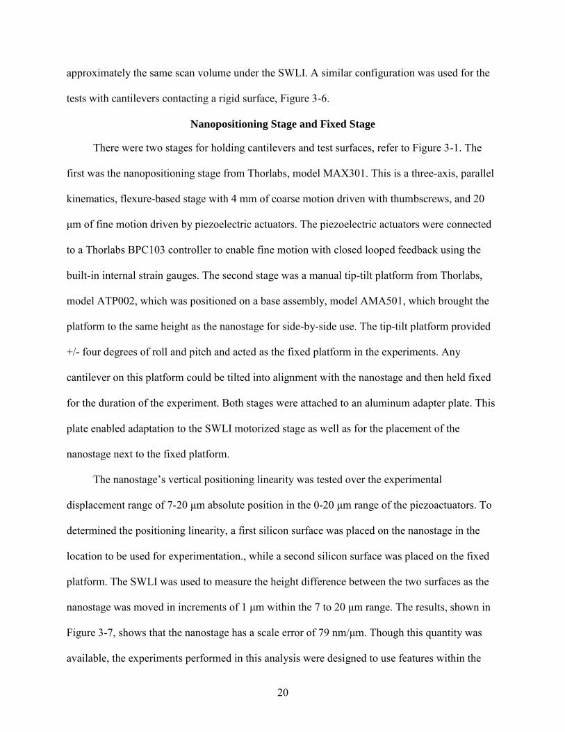
the SWLI sample stage, Figure 3-1.
Scanning White Light Interferometer
A key component in the test setup is the scanning white light interferometer (SWLI). The
SWLI is an optical three-dimensional, or 3D, surface profiler which uses the short coherence
length of white light in order to limit interference to a short depth in the focal region of the
objective. Light reflected from the sample within the focal region will then interfere with light
reflected from a reference surface based on its distance from the objective, Figure 3-2. When the
objective is translated vertically away from the sample the region of interference will also
translate and a 3D reconstruction can be generated to show a surface map of the sample within
the field of view of the objective. The interference fringes are detected by a 640x480 pixel
camera which maps the intensity into vertical position data on a per-pixel basis. Each pixel of the
camera is then a lateral position of the sample, which is dependent on the zoom level and the
objective being used.
There are limitations associated with SWLI measurements. The first is that the lateral
resolution is orders of magnitude higher than the vertical resolution. For our experiments we
used a 20x Mireau objective, which yielded a system magnification of 400x, and varied the zoom
so that our lateral resolution was between 280-710 nm/pixel. In addition, the SWLI cannot detect
19
large height changes between adjacent points, so there is a maximum slope that can be detected.
For the 20x objective, this slope varies depending on zoom level and can be between 18-23
degrees.
The SWLI used in our project was the Zygo NewView 5010 which comes with a
motorized X/Y/tip/tilt stage for sample alignment. The NewView claims a vertical resolution of
0.1 nm; however, tests were performed to determine the repeatability for our experimental setup.
A smooth silicon surface was placed on the nanostage in the cantilever loading location and 130
scans were taken using a 40 μm vertical scan, Figure 3-3. We then determined the height
repeatability for each pixel. It was found that, on average, each pixel reported the same position
within a standard deviation of 2.7 nm. Therefore, we have set the noise floor to this value and
assumed a resolution of the same amount.
Cantilevers and Holders
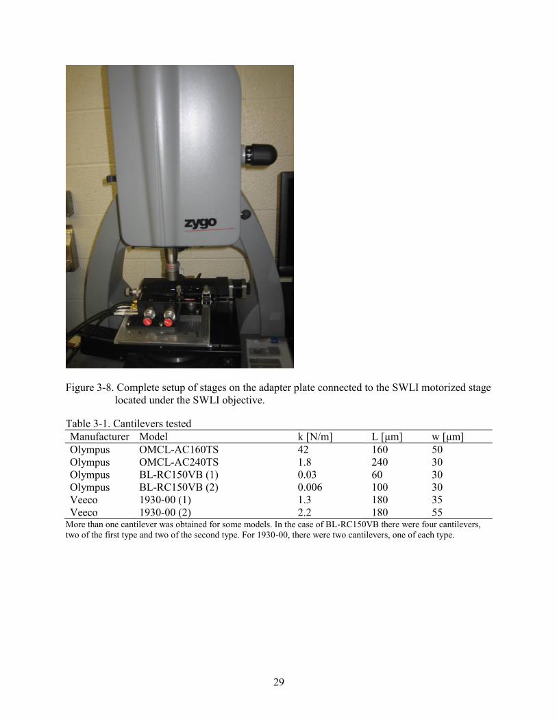
The cantilevers tested were obtained from Olympus and Veeco; they are summarized in
Table 3-1. They were glued with Loctite adhesive to aluminum holders with dimensions of 60
mm x 60 mm and 3 mm thick, Figure 3-4. There was an extra feature machined into each holder,
which is for future work, and will allow precise alignment of cantilevers mounted to the holders.
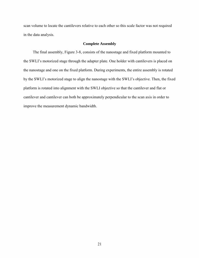
This feature will accept a 20 mm x 20 mm silicon microholder, Figure 3-5. Then the silicon
microholder will accept standard AFM cantilevers. Cantilevers adhered to the silicon
microholder will be easy to manipulate easing experimentation. However, for this experiment,
cantilevers were glued to the sides that did not contain features, Figure 3-4, in order to ensure
each cantilever was on an identical surface. Also, the mid-point of each side was located and
each cantilever was placed at this position. This design allowed the holder to be unscrewed and
rotated to select the next cantilever for experimentation while keeping each cantilever within
20
approximately the same scan volume under the SWLI. A similar configuration was used for the
tests with cantilevers contacting a rigid surface, Figure 3-6.
Nanopositioning Stage and Fixed Stage
There were two stages for holding cantilevers and test surfaces, refer to Figure 3-1. The
first was the nanopositioning stage from Thorlabs, model MAX301. This is a three-axis, parallel
kinematics, flexure-based stage with 4 mm of coarse motion driven with thumbscrews, and 20
μm of fine motion driven by piezoelectric actuators. The piezoelectric actuators were connected
to a Thorlabs BPC103 controller to enable fine motion with closed looped feedback using the
built-in internal strain gauges. The second stage was a manual tip-tilt platform from Thorlabs,
model ATP002, which was positioned on a base assembly, model AMA501, which brought the
platform to the same height as the nanostage for side-by-side use. The tip-tilt platform provided
+/- four degrees of roll and pitch and acted as the fixed platform in the experiments. Any
cantilever on this platform could be tilted into alignment with the nanostage and then held fixed
for the duration of the experiment. Both stages were attached to an aluminum adapter plate. This
plate enabled adaptation to the SWLI motorized stage as well as for the placement of the
nanostage next to the fixed platform.
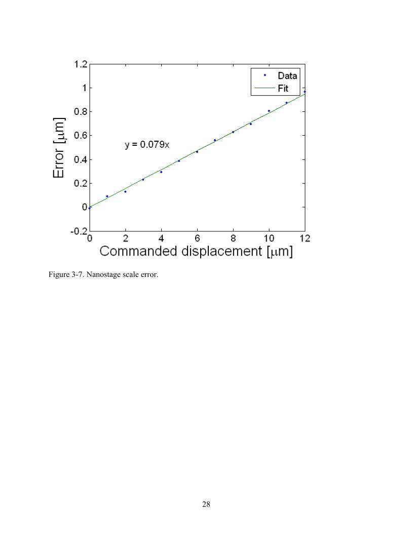
The nanostage’s vertical positioning linearity was tested over the experimental
displacement range of 7-20 μm absolute position in the 0-20 μm range of the piezoactuators. To
determined the positioning linearity, a first silicon surface was placed on the nanostage in the
location to be used for experimentation., while a second silicon surface was placed on the fixed
platform. The SWLI was used to measure the height difference between the two surfaces as the
nanostage was moved in increments of 1 μm within the 7 to 20 μm range. The results, shown in
Figure 3-7, shows that the nanostage has a scale error of 79 nm/μm. Though this quantity was
available, the experiments performed in this analysis were designed to use features within the
21
scan volume to locate the cantilevers relative to each other so this scale factor was not required
in the data analysis.
Complete Assembly
The final assembly, Figure 3-8, consists of the nanostage and fixed platform mounted to
the SWLI’s motorized stage through the adapter plate. One holder with cantilevers is placed on
the nanostage and one on the fixed platform. During experiments, the entire assembly is rotated
by the SWLI’s motorized stage to align the nanostage with the SWLI’s objective. Then, the fixed
platform is rotated into alignment with the SWLI objective so that the cantilever and flat or
cantilever and cantilever can both be approximately perpendicular to the scan axis in order to
improve the measurement dynamic bandwidth.
22
Figure 3-1. Computer generated image of the experimental setup.
23
Figure 3-2. Schematic of SWLI operation.
24
Figure 3-3. Example scan of the smooth silicon surface. The 6 μm difference from lowest to
highest point is a result of contamination on the surface, possibly dust.
25
Figure 3-4. Example cantilever placement on the aluminum holders. Individual cantilevers are too small to see but the monolithic base chips are labeled (A1-C2). If the holders were unscrewed and rotated in the indicated direction, the next experiment would be C1 against C2.
26
Figure 3-5. The silicon holder nests against the machined feature in the aluminum holder. The cantilever A is nested against the micromachined slot in the silicon holder. Artifact B rests in a similar position. Though the cantilever and artifact aren’t visible, their
monolithic base chips are labeled (A,B).
27
Figure 3-6. Example cantilever and silicon surface (S) placement on the aluminum holders. The cantilevers are too small to see but the monolithic base chips are labeled (A-C). If the holder on the left was unscrewed and rotated, the next experiment would be C against S.
28
Figure 3-7. Nanostage scale error.
29
Figure 3-8. Complete setup of stages on the adapter plate connected to the SWLI motorized stage located under the SWLI objective.
More than one cantilever was obtained for some models. In the case of BL-RC150VB there were four cantilevers, two of the first type and two of the second type. For 1930-00, there were two cantilevers, one of each type.
30
CHAPTER 4 EXPERIMENTAL PROCEDURE
Two types of experiments were performed. In the first experiment, the full field
displacement of commercially available cantilevers was observed while pressing the cantilevers
against a rigid surface. This established a comparison baseline for the cantilever pressing on
cantilever tests. A polished silicon wafer was used as the rigid surface. In the second experiment,
cantilevers were pressed against compliant surfaces, i.e., other cantilevers. Given the large
stiffness variation between cantilevers, this experiment simulated pressing against surfaces that
ranged from relatively stiff to very compliant. Also, since cantilever to cantilever calibration is
being investigated at NIST, this was a good test to expose any deviation from expected behavior
during such a calibration.
In the following sections the cantilevers will be referred to by a symbolic designation
which is described in Table 4-1 and Figure 4-1. There were several models of cantilevers which
were tested, including duplicates of each model. Additionally, there was more than one
cantilever on the chip for selected model. Therefore, the designation was separated into three
parts: LetterNumber1-Number2, where Letter represents the cantilever model, Number1
represents which duplicate, and Number2 represents the individual cantilever on a particular
chip.
Cantilever against a Rigid Surface
The first experimental setup was cantilever A mounted on the nanostage and a polished
silicon section mounted on the fixed stage. Cantilever A was then lowered into contact with the
fixed silicon, Figure 4-2. A SWLI scan which could capture the entire cantilever, as well as the
silicon surface, in one image was initially believed to be the best test method. This would enable
the surface to be used as a reference, or fiducial, which could aid in locating features on the
31
cantilever between multiple scans. Because the contacting tip of cantilever A was ~17 μm long,
the gap between the cantilever and silicon piece would need to exceed 17 μm to start the test. To
capture both objects, the vertical scan length of the SWLI would have to be at least 20 μm;
however, it was found that a scan length of 40 μm (the next available scan length in the SWLI
software) was required. In addition, the nanostage was moved in 50 nm increments towards the
cantilever in an attempt to capture snap-in and provide good resolution for data analysis. The
combination of long vertical scans, averaging to reduce noise (10 times per stage position), and
significant stage travel range (several micrometers), yielded a single test time that approached
several hours. In the interest of time, the method was modified for the remaining three
cantilevers.
Cantilevers B and C were mounted on the fixed stage and a polished silicon section was
mounted on the nanostage. Then, the silicon was placed under the cantilever and pressed up
against the tip, Figure 4-3. The intent was that since the cantilevers were on the fixed stage they
would appear in the same location in every scan and the location of features on one cantilever
would be valid for subsequent scans of the same cantilever. This would reduce the scan length
since the silicon surface would not need to be in the scan volume. Unfortunately, after each scan
the objective does not return to exactly the same position so this did not work. However, another
method for analyzing the data was developed and is outlined in the data analysis section.
Alignment for each cantilever was performed using the SWLI. Since the cantilevers
themselves had irregular shapes due to residual stress from thin film deposition, their surfaces
were not used for alignment. Instead, the chip which forms the base of the cantilever was used
because the bases are monolithically attached to the cantilevers and should be very close to
parallel with the cantilevers. An example of alignment using the interference fringes on the
32
cantilevers is shown in Figure 4-4. The fringes on the chip on the nanostage are at first bunched
together showing that there is a steep height change in the focal region. Rotating the SWLI’s
motorized stage starts to level the surface which increases the fringe spacing. Finally, only one or
two fringes are left when the surface is well aligned showing that there is no appreciable height
difference across the surface of the chip. The process was repeated on the chip attached to the
fixed stage. However, the manual tip-tilt mechanism on the fixed stage was used for alignment.
The steps required for the experiments are listed below.
Adhere the silicon piece to one holder and the cantilevers to the other holder
Mount the holders to their stages and align each to the SWLI
Use the coarse motion of the nanostage to move the cantilever and silicon within the field of view
Using the focal plane of the objective as a guide, raise the cantilever to a height above the silicon and then move the cantilever over the silicon
Using a few SWLI scans as a guide, lower the cantilever over the silicon until touching (the end of the cantilever as imaged by the SWLI will either move if the cantilever is on the fixed stage or stop moving if the cantilever is on the nanostage)
Using the Thorlab’s ATP software virtual instrument to control the nanostage fine motion actuator, move the stage away from the cantilever by a few micrometers to cause the cantilever tip to hover just over the silicon surface
Finally, lower the cantilever or raise the silicon surface in increments of 50-100 nm, taking ten 10-40 μm scans per increment. Move the stage until there has been several micrometers
of cantilever deflection (difference in height between the end of the cantilever and the base)
Cantilever against Cantilever
These experiments were similar to the previous tests with some minor changes that reflect
improvements implemented after the first study. Since both cantilevers were of interest, the scan
length of the SWLI was increased to a value of 40 μm to capture both cantilevers in one scan.
Also, the total distance the nanostage moved was increased from a few micrometers to 10 μm in
33
order to provide more bending of the cantilevers. For stiff versus flexible combinations, this
would yield cantilever end deflection of nearly 10 μm for the more flexible beam. To keep the
time to perform experiments reasonable, the stage was moved in increments of 1 μm, Figure 4-5.
None of the cantilevers from the previous experiments were reused. The total possible
combinations of cantilevers were very large so only a select number of combinations were tested,
as shown in Table 4-2. The first experiment identified any potential bias that could exist between
the fixed side and the moving side. The remaining experiments included each cantilever model
pressed against cantilevers that covered the full stiffness range of 0.006 N/m to 42 N/m with one
exception. Only when experiments for cantilevers B1-21 and B1-22 are combined do they cover
the full stiffness range; cantilevers B1-21 and B1-22 were nominally identical cantilevers on the
same chip so this was possible.
The experimental procedure was nearly identical to the previously described approach.
Adhere the #1 cantilevers to one holder and the #2 cantilevers to the other in the manner described in Chapter 3
Mount the #1 cantilevers to the nanostage and the #2 cantilevers to the fixed stage (except reverse for experiment A2 against A1) and perform alignment
Use the coarse motion of the nanostage to move both cantilevers into the field of view
Using the focal plane of the objective as a guide, move the nanostage cantilever to a height above the fixed cantilever and then move the nanostage cantilever over the fixed cantilever
Focus on the fixed cantilever so that interference fringes appear and then slowly lower the nanostage with the coarse motion drive until the fringes on the fixed cantilever begin to move. This indicates the cantilever is beginning to deflect due to the surface forces pulling at it from the other cantilever
Finally, perform ten 40 μm long scans per 1 μm increment of fine motion for 10 μm
34
Figure 4-1. Schematic of each cantilever used in the experiments with their designations.
35
Figure 4-2. Schematic of the first cantilever for the first experiment
Figure 4-3. Schematic of the remaining cantilevers for the first experiment.
36
Figure 4-4. Aligning the cantilevers with the SWLI objective. Align the cantilever on the nanostage (1-3) and then the cantilever on the fixed stage (4-6). When only one or two interference fringes can be seen the cantilevers are aligned (3 and 6).
For the first experiment there were no duplicates so the cantilevers are described by Letter-Number combinations. The second experiment included duplicate cantilevers so the designations include LetterNumber1-Number2 combinations. Also, k is the manufacturer reported stiffness of the cantilevers.
Cantilevers on the nanostage were push against cantilevers on the fixed platform. The first experiment identifies any potential bias from being the pushee versus the pusher.
39
CHAPTER 5 DATA ANALYSIS
Euler-Bernoulli Beam Fit
The research objective was to compare the bending profile of cantilever bending shapes
(against both the rigid surface and other cantilevers) with the profile described by the fixed-free
Euler-Bernoulli beam bending equation with the force applied at the free end. The form of the
equation is
2( ) 36
Fy x x L x
EI , (1)
where y is the transverse deflection of the cantilever, x is the distance along the length of the
beam, L is the total length of the beam (measured by the SWLI), F is the force applied at the
tip, E is the modulus of elasticity of the beam, and I is the moment of inertia of the beam. Also,
using the relationship that the stiffness
Fk
y when x L , (2)
then 3
3
kLEI , where k is the stiffness value specified by the manufacturer. In the analysis, the
beam deflection data is used to determine a least square best fit to Eq. (1) in order to determine a
value for F . The F value can also be determined from Eq. (2) using the manufactured specified
value for k and measured y value at the tip. While the accuracy of the F values may be limited
by the manufacturer’s k value, as long as Eq. (1) makes a good fit then the cantilever is behaving
as an Euler-Bernoulli beam with fixed-free boundary conditions. If the fit of the data is poor,
then the beam may have a complex boundary condition at the tip and new expressions would be
required for force calculation.
40
Cantilever Profile Extraction
This section describes the process of transforming SWLI data into a form compatible for
fitting using Eq. (1). Each cantilever had a pre-strained (non-planar) shape, presumably due to
post-processing residual stresses. Therefore, a reference scan was performed under zero load
condition and subsequently differenced from every other scan to obtain the relative motion of
each point along the beam. The differencing process was not straightforward because, over the
course of an experiment, the cantilevers would shift several pixels laterally, Figure 5-1:
consequently, a direct pixel-by-pixel difference could not be completed.
Also, for each SWLI scan the full field view of the cantilever had to be sectioned down the
middle to extract the bending profile, Figure 5-2. After sectioning, the profile was not in the
same coordinate system used by Eq. (1). Sometimes the cantilever was reversed as in Figure 5-2,
and the cantilever base was never located at ( 0x , 0y ). Finally, there were outliers in each
profile due to the SWLI’s inability to accurately measure steep slopes. This occurred frequently
at the base and the tip, but sometimes also occurred along the length of the profile, possibly due
to dust or other contamination.
The entire analysis process was automated in MATLAB. The algorithms which were
developed helped reduce human bias in the process and enabled rapid analysis. The data analysis
steps are provided here for the first experiments,
Reverse the image to match Eq. (1), if necessary
Isolate cantilever data and adjust for lateral shift of the type in Figure 5-1
Perform a pixel-by-pixel difference with the reference image
Find the tip of the cantilever and perform horizontal sectioning (Figure 5-2, straight line section)
Shift the section so that the base is at 0x
41
Shift the section so that the base is at 0y (this is discussed in the next section)
Perform least squares fit to Eq. (1) and calculate the error
The process was changed for the second set of experiments. First, the new data had two
cantilevers in the same view which needed to be separated. Second, there was the addition of a
new type of cantilever that did not have an obvious base location, Figure 5-3. Finally, the
sectioning process was improved to better handle misaligned cantilevers. The following process
was used for the second experiments,
Find the base of the cantilever and then take a section down the middle of the cantilever stopping at the tip (this effectively aligns the data for differencing and separates the cantilevers in one move), Figure 5-4
Difference the section from the reference image and then reverse the section to match Eq. (1), if necessary
Shift the section so that the base is at 0x
Shift the section so that the base is at 0y (discussed in the next section)
Perform a fit to Eq. (1) and calculate error
Profile Shifting
Shifting the section bases to 0y was not as straightforward as it was for the 0x shift.
For the x-axis, the first pixel that had valid data was assumed to be the base or, in a case like
Figure 5-4, the base was calculated from a line fit to the flange edges. However, noise in the y-
axis data, Figure 5-5, can adversely affect selection of the first point to represent the base at
0y . In order to remove this noisy data, an outlier rejection algorithm was applied. This
algorithm performed a polynomial curve fit to the data and points “far away” were removed,
Figure 5-6. This was an iterative process where “far away” was quantified by the statistical
definition for outliers. If 1Q and 3Q are the first and third quartiles and 3 1IQR Q Q is the
interquartile range, then the outer fence of the data is
42
3 1.5Data Q IQR
for mild outliers and
3 3Data Q IQR
for extreme outliers [27]. After outlier rejection, a final polynomial curve was fit to the
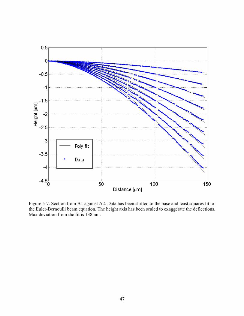
remaining data and evaluated at 0x . This best fit point was used to shift the data along the y-
axis. See Figure 5-7 for example results from the full analysis procedure completed for cantilever
on cantilever data.
43
Figure 5-1. Lateral misalignment in the data. Axes are in pixels.
44
Figure 5-2. Example view of cantilever in contact with a silicon surface (1), the SWLI surface map (2), and the cross-section used for data analysis (3).
Figure 5-3. The cantilever on the left has a base that merges with a larger piece at (1), while the cantilever on the right has its base located at the last point before data dropout (2).
45
Figure 5-4. The base line defines the starting point of the cantilever and is calculated by a line fit to the flange edges. The section line defines the location of the 2D section for comparison to the bending equation. The thick line on top of the section line is the data belonging to the left cantilever. A new section line is calculated for the right cantilever.
46
Figure 5-5. Height data is noisy at the base (1 and 2). The vertical offset between the right end of the left cantilever and the left end of the left cantilever is due to the tip height.
Figure 5-6. Refinement process on one cantilever. In each iteration the outliers are identified and marked. The data that remains for the next fit is marked as refined. Each iteration reconsiders all data so that points marked as outliers before may be kept later. The final iteration uses the most lenient definition for outliers to keep as many points as possible.
47
Figure 5-7. Section from A1 against A2. Data has been shifted to the base and least squares fit to the Euler-Bernoulli beam equation. The height axis has been scaled to exaggerate the deflections. Max deviation from the fit is 138 nm.
48
CHAPTER 6 RESULTS AND DISCUSSION
Cantilevers were compared to the Euler-Bernoulli beam equation by comparing points in
the data with the corresponding points generated by the beam equation; see Figure 6-1 for the
coordinate system. For any point along the distance-axis ix , compute 2 36
i i i
Fy x L x
EI along
the height-axis using the values for the constants as mentioned in the previous chapter. Next,
collect the measured value iY that corresponds with ix and the root mean square (RMS) error is
then max
2
1 max
ii i
i
y Y
i
where maxi is the last element in a profile. A quantity that will be used often
is the RMS percent which is the RMS error divided by the maximum tip displacement, maxiY .
This value is roughly constant over the range of tip displacements showing that the RMS error
rises linearly with the maximum tip displacement. The last metric is the full error profile which
is the absolute error, i iy Y plotted against ix for max1 i i . The shape of the error profile can
help determine what the most important error source is and will be discuss later.
Cantilever against Rigid Surface
Overall the tests showed that there was good conformation of the cantilever bending shape
to the Euler-Bernoulli fixed-free beam equation. The curve fit for cantilever C1 had the best
agreement to the beam fit, Figure 6-1, except at curve 1 where the tip deflection approached zero
resulting in a higher RMS percent relative to the tip deflection (~3% compared to ~0.5%). Curve
5 represents the maximum free end displacement (and load). Additional results are provided in
Appendix A. In general, the RMS error increased linearly with tip displacement (neglecting the
special case of near zero displacement). Also, bending near the base is clearly visible while there
appears to be no bending in the tip which is consistent with the fixed-free boundary condition.
49
Cantilever B was the exception to the above, seen in Figure 6-2. It showed no bending at any
point along its length; it moved as though on a hinge. In addition, it had a non-constant RMS
percent. It is believed that the cantilever was cracked at the base. However, the cantilever was
destroyed prior to examination using a scanning electron microscope. Coincidentally, cantilever
B was the only cantilever mounted on the nanostage and so, in the next section, one pair of
cantilevers were tested, the stages were swapped, and then the cantilevers were retested to ensure
the equality of mounting locations. The analysis of cantilever B was a good illustration of the
robustness of using a full field displacement map because it highlighted the unusual bending
behavior that may not have easily been detected with a single point laser measurement.
Cantilever against Cantilever
In general, this experiment showed similar patterns and error levels as the previous
experiment. The first test showed similar behavior when reversing the same cantilever to a
different stage, Figure 6-3 and Figure 6-4. However, in comparing the two measurements, Figure
6-5, it was found that when the cantilever was placed on the bottom it appeared slightly stiffer
(had less tip deflection). This small discrepancy was expected due to the sensitivity to the
location of load application for fixed-free beams. For the top cantilever the load acts through the
tip, providing repeatable results. However, for the bottom cantilever the load point occurs where
the top cantilever comes into contact on its surface. Since the top cantilever appears in the direct
line of sight of this point it is difficult to obtain accurate alignment.
A summary of the rest of the experiments shows good agreement between the data and the
curve fit, Table 6-1. The table shows the maximum deflection attained for each cantilever and
the associated errors. There are a few cantilevers with large percent errors, for example C1-2 for
the C1-2 against B2-21 test. Comparing the profiles of C1-2 at minimum and maximum
deflections, Figure 6-6, it is seen that the data scatter (for the beam section along its centerline)
50
has increased dramatically. Also, for the absolute error plot of B2-21, Figure 6-7, a discontinuity
is observed. The discontinuity in Figure 6-7 is indicative of a vibration to the system and since
both cantilevers were affected it is a likely candidate for explaining the extra spread in C1-2.
Inspecting C2-1 from the B1-11 on C2-1 test and from the B1-12 on C2-1 test shows similar
spread (figures included in appendix A). It is possible the reason the C1 and C2 cantilevers are so
sensitive to vibration is that they are very long, have a relatively large volume (mass), and a
relatively low stiffness. This helps them to couple onto inertial disturbances. The noisy behavior
only occurs when C1 and C2 cantilevers are contacting the B1 and B2 cantilevers, i.e: very
compliant cantilevers.
Expected Errors
There were several error contributors for the comparison between beam theory and
measurement of the cantilever profiles under load. The cantilever length measurement was
limited by three primary factors. First, the resolution of the SWLI, which varied depending on
the zoom level, was 280 nm/pixel to 710 nm/pixel. Second, there was an effect of data dropout at
the edge of the cantilever, Figure 6-7. The data loss was up to 10-15 pixels, which leads to a
length deviation between 2.8-10.7 μm. Third, the length of the cantilever was also affected by the
selection of base location. For most cantilevers the base was assumed to be at the edge of data
dropout. The true base location is more difficult to identify. It depends on whether the cantilever
was properly registered during microfabrication and also depends on the severity of undercut. A
scanning electron microscope image of an OMCL-AC160TS cantilever is provided in Figure 6-
9; the undercut at the base is observed. Also, since the cantilevers were not rectangular (some
models had narrowing at the end into a point) there will be some deviation from beam theory.
Assume there was a perfectly behaved cantilever with the dimensions of the OMCL-
AC160TS, 42k N/m, being deflected by 5 μm at the tip. The errors described above can be
51
applied to this ideal cantilever and compared against the actual errors seen in the analysis. Given
a length miscalculation of 10 μm from ideal, and attempting to fit the Euler-Bernoulli beam
equation gives an RMS error of only 7 nm, Figure 6-10. Next, assume the cantilever base was
miscalculated by 10 μm (possibly due to undercut), Figure 6-11. The RMS error is now 89 nm,
Figure 6-12, and the error curve has a distinctly different shape. The actual RMS error for this
cantilever, given the same tip deflection is 61 nm, Figure 6-13. The shape of the actual error
curve is more indicative of base miscalculation than length miscalculation.
52
Figure 6-1. Cantilever C1 pressed against the silicon surface. RMS error is linearly dependent on tip deflection.
Figure 6-2. Cantilever B against the silicon surface. RMS error has no clear relationship to tip deflection and the curve fit is very different from the actual data. Cantilever damage at the base was inferred.
53
Figure 6-3. Cantilever A1 from test A1 on A2. The RMS error is linearly dependent on tip deflection.
Figure 6-4. Cantilever A1 from test A2 on A1. The RMS error is again linearly dependent on tip deflection. No hinge behavior as with the previous cantilever against rigid surface test for the same stage configuration.
54
Figure 6-5. Comparison of the same cantilever when in the top position (pusher) versus the bottom position (pushee). The bottom position makes the cantilever appear stiffer.
Figure 6-6. Cantilever C1-2 shows a sudden increase in data spread from tip position (1) to (2).
55
Figure 6-7. Absolute value of error for cantilever B2-21 during the C1-2 on B2-21 test. The discontinuity at (1) suggests the cantilevers experienced a vibration.
Figure 6-8. Cantilever length measuring error. The true edge of the cantilever is invisible to the SWLI since the edge is too steep to detect (1). Using a surface underneath as a backdrop the missing edge is exposed (2).
56
Figure 6-9. SEM image of undercut at the base.
57
Figure 6-10. Error curve if a perfect OMCL-AC160TS had a length error of 10 μm. RMS error is
7 nm.
58
Figure 6-11. Cantilever with profile data set to the depicted coordinate system. Actual coordinate system should be 10 μm further back.
59
Figure 6-12. Error curve if a perfect OMCL-AC160TS had an error locating the base by 10 μm.
RMS error is 89 nm.
60
Figure 6-13. Error of an actual OMCL-AC160TS at similar deflection as the perfect OMCL-AC160TS in Figure 6-12. RMS error is 61 nm.
61
Table 6-1. Error summary for each cantilever combination
Reported errors are for the maximum tip deflection achieved by each cantilever
62
CHAPTER 7 CONCLUSIONS
In our work, an experimental setup was developed for measuring the full field
displacement of AFM cantilevers during loading. The setup included a nanopositioning stage to
provide relative motion between cantilevers or a cantilever and rigid surface, a fixed stage with
tip-tilt control for parallel alignment with the nanostage, and a SWLI for measuring the
cantilever displacement. The setup also featured holders for the cantilevers which could be
removed and rotated to select various cantilever combinations for testing. Data analysis was
completed using algorithms designed to remove human bias from the two-dimensional
sectioning and outlier rejection process.
Experiments were conducted on several commercially available cantilevers. These
cantilevers were end-loaded and their full field deflections measured and compared to the Euler-
Bernoulli beam equation with fixed-free boundary conditions. Two sets of experiments were
performed: one for cantilevers contacting a rigid surface and another for cantilevers contacting
other cantilevers. Agreement with the assumed beam model is demonstrated in Figure 7-1 and
Table 7-1; the root mean square (RMS) error between the measured data and the theoretical
model is rank-ordered and the system compliance is listed. The system compliance was
calculated as
1 1 1
system nanostage fixed stagek k k where nanostagek is the stiffness of the cantilever on the
nanostage and fixed stagek is the stiffness of the cantilever on the fixed stage. Most cantilevers had
a constant RMS error over tip displacement which ranged between ~0.5% to ~4%. It is seen that
no clear trend is exhibited with change in the system compliance. The overall reasonable
agreement suggests that the fixed-free Euler Bernoulli beam model is acceptable for describing
the cantilever behavior under typical loading conditions.
63
There were a few exceptions that had higher errors, between ~8% and ~223%. One
cantilever was found to bend as though connected to the base by a hinge and was presumed
damaged (max error of 28%). This highlighted the ability of the measurement experimental
technique to identify anomalies. Another cantilever had tip deflections near the noise floor and
so did not give reliable data. There were also cantilevers that were potentially exposed to
vibrations during experimentation which increased the spread in the collected data.
After performing several experiments, limitations were exposed. Length could not be
measured well due to the physical limitations of the SWLI at sharp edges and the low lateral
resolution of the objective. In addition, the top cantilever blocked the view of the bottom
cantilever during alignment. For these reasons, cantilevers could not be aligned precisely at the
edges forcing the load to be applied at a point closer to the base. This resulted in one cantilever
appearing stiffer than nominal. Also, the base location was found to be a sensitive parameter to
error.
In future work the process of locating the cantilever base should be refined to try to
eliminate this error source. In addition, experiments should be performed in vacuum to
encourage stronger surface bonding at the cantilever tip, which may affect the boundary
condition. Another way to test the tip would be to introduce new surfaces with which the
cantilevers could interact, such as biological samples. Once competence is achieved, the next
step would be to carry out cantilever calibration using pre-calibrated artifacts that have a load
zone which is insensitive to load application position.
64
Figure 7-1. Rating of cantilevers given their system compliance. The RMS percent error is included for the cantilevers mounted to both the fixed stage and nanostage at each level of system compliance (which depends on the stiffness of both).
Table entries are for the maximum tip deflection per cantilever.
67
APPENDIX A CANTILEVER TRIALS
Cantilever against Rigid Surface
This section holds the other results of cantilever C2 on a rigid surface and cantilever A on
a rigid surface. These cantilevers showed good conformity to the Euler-Bernoulli curve fit for a
fixed-free beam. Figure A-1 has near constant RMS percent but is always deflected off of the
distance-axis. Figure A-2 shows what happens when the deflection on the distance-axis, the
RMS percent for curve 1 is ~223%. This is because tip deflection appears in the denominator and
for curve 1 the tip is nearly zero deflection.
Figure A-1. Cantilever C2 against the silicon surface. RMS error is linearly dependent on tip deflection.
68
Figure A-2. Cantilever A against the silicon surface. RMS error is linearly dependent on tip deflection except for curve 1 where the tip deflection approaches zero.
Cantilever against Cantilever
Cantilevers could experience a sudden increase in spread. Sometimes the spread would last
for the entire experimental set suggesting that if there were ambient vibrations, this combination
of cantilevers was most sensitive to them. Figures A-3 and A-4 show examples of two entire test
runs where large spreads were observed.
69
Figure A-3. Cantilever C2-1 from B1-11 against C2-1. Significant spread in the data is observed.
Figure A-4. Cantilever C2-1 from B1-12 against C2-1. Significant spread in the data is observed.
70
LIST OF REFERENCES
1. Gibson CT, Watson GS, Myhra S (1996) Determination of the spring constants of probes for force microscopy/spectroscopy. Nanotechnology 7:259-262.
2. Poggi MA, McFarland AW, Colton JS, Bottomley LA (2005) A method for calculating the spring constant of atomic force microscopy cantilevers with a nonrectangular cross section. Analytical Chemistry 77:1192-1195.
3. Blank K, Mai T, Gilbert I, Schiffmann S, Rankl J, Zivin R, Tackney C, Nicolaus T, Spinnler K, Oesterhelt F, Benoit M, Clausen-Schaumann H, Gaub HE (2003) A force-based protein biochip. PNAS 100:11356-11360.
4. Cleveland JP, Manne S, Bocek D, Hansma PK (1993) A nondestructive method for determining the spring constant of cantilevers for scanning force microscopy. Review of Scientific Instruments 64:403-405.
5. Sader JE, Pacifico J, Green CP, Mulvaney P (2005) General scaling law for stiffness measurement of small bodies with applications to the atomic force microscope. Applied Physics 97:124903.
6. Gibson CT, Weeks BL, Lee JRI, Abell C, Rayment T (2001) A nondestructive technique for determining the spring constant of atomic force microscope cantilevers. Review of Scientific Instruments 72:2340-2343.
7. Gibson CT, Johnson DJ, Anderson C, Abell C, Rayment T (2004) Method to determine the spring constant of atomic force microscope cantilevers. Review of Scientific Instruments 75:565-567.
8. Golovko DS, Haschke T, Wiechert W, Bonaccurso E (2007) Nondestructive and noncontact method for determining the spring constant of rectangular cantilevers. Review of Scientific Instruments 78:043705.
9. Notley SM, Biggs S, Craig VSJ (2003) Calibration of colloid probe cantilevers using the dynamic viscous response of a confined liquid. Review of Scientific Instruments 74:4026-4032.
10. Butt H, Jaschke M (1995) Calculation of thermal noise in atomic force microscopy. Nanotechnology 6:1-7.
11. Cumpson PJ, Hedley J, Zhdan P (2003) Accurate force measurement in the atomic force microscope: a microfabricated array of reference springs for easy cantilever calibration. Nanotechnology 14:918-924.
12. Cumpson PJ, Hedley J, Clifford CA, Chen X, Allen S (2004) Microelectromechanical system device for calibration of atomic force microscope cantilever spring constants between 0.01 and 4 N/m. Vacuum Science and Technology A 22:1444-1449.
71
13. Cumpson PJ, Clifford CA, Hedley J (2004) Quantitative analytical atomic force microscopy: a cantilever reference device for easy and accurate AFM spring-constant calibration. Measurement Science and Technology 15:1337-1345.
14. Torii A, Sasaki M, Hane K, Okuma S (1996) A method for determining the spring constant of cantilevers for atomic force microscopy. Measurement Science and Technology 7:179-184.
15. Newell DB, Kramar JA, Pratt JR, Smith DT, Williams ER (2003) The NIST Microforce Realization and Measurement Project. Transactions on Instrumentation and Measurement 52:508-511.
16. Pratt JR, Smith DT, Newell DB, Kramar JA, Whitenton E (2004) Progress toward Système International d’Unités traceable force metrology for nanomechanics. Materials
Research 19:366-379.
17. Gates RS, Pratt JR (2006) Prototype cantilevers for SI-traceable nanonewton force calibration. Measurement Science and Technology 17:2852-2860.
18. Holbery JD, Eden VL, Sarikaya M, Fisher RM (2000) Experimental determination of scanning probe microscope cantilever spring constants utilizing a nanoindentation apparatus. Review of Scientific Instruments 71:3769-3776.
19. Cumpson PJ, Hedley J (2003) Accurate analytical measurements in the atomic force microscope: a microfabricated spring constant standard potentially traceable to the SI. Nanotechnology 14:1279-1288.
20. Proksch R, Schäffer TE, Cleveland JP, Callahan RC, Viani MB (2004) Finite optical spot size and position corrections in thermal spring constant calibration. Nanotechnology 15:1344-1350.
21. Aksu SB, Turner JA (2007) Calibration of atomic force microscope cantilevers using piezolevers. Review of Scientific Instruments 78:043704.
22. Gibson CT, Smith DA, Roberts CJ (2005) Calibration of silicon atomic force microscope cantilevers. Nanotechnology 16:234–238.
23. Matei GA, Thoreson EJ, Pratt JR, Newell DB, Burnham NA (2006) Precision and accuracy of thermal calibration of atomic force microscopy cantilevers. Review of Scientific Instruments 77:083703.
24. Cook SM, Scäffer TE, Chynoweth KM, Wigton M, Simmonds RW, Lang KM (2006) Practical implementation of dynamic methods for measuring atomic force microscope cantilever spring constants. Nanotechnology 17:2135-2145.
25. Lévy R, Maaloum M (2002) Measuring the spring constant of atomic force microscope cantilevers: thermal fluctuations and other methods. Nanotechnology 13:33-37.
72
26. Kopycinska-Müller M, Geiss RH, Hurley DC (2006) Contact mechanics and tip shape in AFM-based nanomechanical measurements. Ultramicroscopy 106:466-474.
73
BIOGRAPHICAL SKETCH
Lee Kumanchik was born in Miami, Florida to Dwight and Bunny Kumanchik. He
attended Miami Southridge Senior High School and graduated in June of 2001. Lee joined the
Machine Tool Research Center (MTRC) under the guidance of Dr. Tony Schmitz in October
2004 and was awarded the degree of Bachelor of Science in Mechanical Engineering from the
University of Florida in December 2005. He has since continued research with the MTRC and is
scheduled to complete his master of science degree in August 2007.


![Transverse Vibration Analysis of Euler-Bernoulli Beams ......The vibration problems of uniform and nonuniform Euler-Bernoulli beams have been solved analytically or approximately [1-5]](https://static.documents.pub/doc/80x56/5f7325584196615a4a1178a7/transverse-vibration-analysis-of-euler-bernoulli-beams-the-vibration-problems.jpg)


![An isogeometric collocation approach for Bernoulli–Euler ... · the so-called differential quadrature methods [51–54]. A particular feature of Bernoulli–Euler beam and Kirchhoff](https://static.documents.pub/doc/80x56/602c9703becf5e244842da2c/an-isogeometric-collocation-approach-for-bernoulliaeuler-the-so-called-differential.jpg)


