Page 1
COMPARATIVE ANALYSIS BETWEEN THE DIVERGING DIAMOND
INTERCHANGE AND PARTIAL CLOVERLEAF INTERCHANGE USING
MICROSIMULATION MODELING
by
Borja Galletebeitia
A Thesis Submitted to the Faculty of
The College of Engineering and Computer Science
in Partial Fulfillment of the Requirements for the Degree of
Master of Science
Florida Atlantic University
Boca Raton, FL
December 2011
Page 2
ii
Copyright by Borja Galletebeitia 2011
Page 4
iv
ACKNOWLEDGEMENT
Foremost, I would like to express my thanks and appreciation to my advisor, Dr.
Evangelos I. Kaisar, for guiding and helping me throughout this process and for allowing
me to be part of his transportation research group. Dr. Kaisar’s knowledge and oversight
were vital for the completion of this thesis. I would also like to acknowledge and thank
Gilbert Chlewicki and Dr. Joe Bared for their suggestions and inputs in this research. In
addition, I would like to thank Dr. Stevanovic, Dr. K. Sobhan and Ms. J. Rodriguez-Seda
for being part of my thesis committee and for sparing their invaluable time reviewing and
providing comments on my thesis.
I also would like to thank all my family for believing, encouraging and supporting
me at every step in my life. Without them, nothing in my life would have been possible.
I also would like to thank everyone in the transportation group who helped me throughout
this process, especially Nikola Mitrovic, Ionnis Psarros, Dusan Milosija Jolovic, Alicia
Benazir Portal, Yueqiong Zhao, Alexandra Suzanne Johnsen and Mary Anise. Finally I
want to show my gratitude to my twin brother who has always been very supportive of
me, and has made this whole experience a much better one.
Page 5
v
ABSTRACT
Author: Borja Galletebeitia
Title: “Comparative Analysis between the Diverging Diamond Interchange and the Partial Cloverleaf Interchange using Micro-Simulation Modeling”
Institution: Florida Atlantic University
Thesis Advisors: Dr. Evangelos I. Kaisar
Degree: Master of Science
Year: 2011
In the last decades, population growth has been outpacing transportation
infrastructure growth, and today’s transportation professionals are challenged to meet the
mobility needs of an increasing population. The effectiveness of the transportation
system is an essential constituent of people’s daily lives as they commute between
different points of interest. Studies show that at many highway junctions, congestion
continues to worsen, and drivers are experiencing greater delays and higher risk
exposures. Engineers have very little resources to handle this increase in population.
One solution to resolve and alleviate congestion due to increasing traffic volumes and
travel demands relies in implementing alternative designs. This approach will help traffic
engineers determine which design will be the most appropriate for a particular location.
This study compares and evaluates the Diverging Diamond Interchange (DDI), which is
an unconventional design, to Partial Cloverleaf (ParClo) types A4 and B4 interchange
Page 6
vi
designs by evaluating different Measure of Effectiveness (MOEs). Using micro-
simulation platform AIMSUN, each interchange type was evaluated for low, medium and
high traffic flows. The analysis revealed that the DDI with four through lanes performed
better than the ParClo A4 for unbalanced conditions, the DDI with six though lanes had
similar results as the ParClo B4 for very high volumes. In terms of queue, the DDI
design had a much better performance. The results from the analysis help in providing
guidelines to the decision makers for selecting the best alternative in terms of
performance.
Page 7
vi
DEDICATION
This thesis is dedicated to my entire family, especially to my mom and my uncle, for their
love, support and encouragement throughout all these years and also because they always
made me believe I could accomplish anything I set my mind to. I will always be grateful.
“Thank you”
Page 8
vii
COMPARATIVE ANALYSIS BETWEEN THE DIVERGING DIAMOND
INTERCHANGE AND PARTIAL CLOVERLEAF INTERCHANGE USING
MICROSIMULATION MODELING
LIST OF FIGURES ........................................................................................................... ix
LIST OF TABLES ............................................................................................................ xii
INTRODUCTION .............................................................................................................. 1
Motivation ....................................................................................................................... 2
Problem Statement .......................................................................................................... 5
Overview of Approach .................................................................................................... 9
LITERATURE REVIEW ................................................................................................. 14
Diverging Diamond Interchange ................................................................................... 14
Partial Cloverleaf ........................................................................................................... 25
Guidelines for Selecting Interchange Type ................................................................... 28
Micro-simulation Platform ............................................................................................ 28
METHODOLOGY ........................................................................................................... 30
Interchange Background ............................................................................................... 32
Diverging Diamond Interchange ............................................................................... 32
Page 9
viii
Partial Cloverleaf ....................................................................................................... 35
Experimental Design ..................................................................................................... 44
Microsimulation Platform.......................................................................................... 44
Measures of Effectiveness ......................................................................................... 47
Geometrical Features ................................................................................................. 49
Safety Analysis .......................................................................................................... 53
Signal Settings and Signal Optimization tool ............................................................ 55
Traffic Volume Scenarios .......................................................................................... 63
Model inputs and development.................................................................................. 67
ANALYSIS AND RESULTS ........................................................................................... 71
CONCLUSION ................................................................................................................. 94
RECOMMENDATIONS FOR FUTURE WORKS ......................................................... 97
APPENDIX ....................................................................................................................... 99
REFERENCES ............................................................................................................... 101
Page 10
ix
LIST OF FIGURES
Figure 1 Projected Vehicle Miles of Travel, 2004-2055 (AASHTO, 2007) ...................... 6
Figure 2 Diverging Diamond Interchange (Chlewicki, 2003) .......................................... 15
Figure 3 Layout of a Diverging Diamond Interchange Design (Bared et. al., 2005) ....... 17
Figure 4 Signal Settings for a DDI (Bared et. al., 2005) .................................................. 18
Figure 5 Conflict Points for a) DDI, b) Diamond Interchange and c) SPUI .................... 20
Figure 6 Traffic Volumes (Speth et. al., 2008) ................................................................. 21
Figure 7 Six Common Types of ParClos (Zhang et. al., 2010) ........................................ 26
Figure 8 Phasing Scheme for ParClo a) Types A and b) Type B (Zhang et. al., 2010) ... 27
Figure 9 Methodology Procedure ..................................................................................... 31
Figure 10 First U.S. Diamond Diverging Interchange (Chlewicki, 2010) ........................ 33
Figure 11 Crossover Movements in a DDI Interchange (Bared, 2009) ............................ 35
Figure 12 Six Types of Partial Cloverleaf (Zhang et. al., 2010) ...................................... 36
Figure 13 ParClo A4 (MnDOT, 2001) .............................................................................. 38
Figure 14 A ParClo A4 Type Interchange on the Highway 407 Electronic Toll
Route in Ontario (www.canadiandesignresource.ca, 2009) ...................................39
Figure 15 ParClo B4 (MnDOT, 2001) .............................................................................. 40
Page 11
x
Figure 16 A ParClo B4 Type Interchange in Woodhaven Wayne, MI ............................. 42
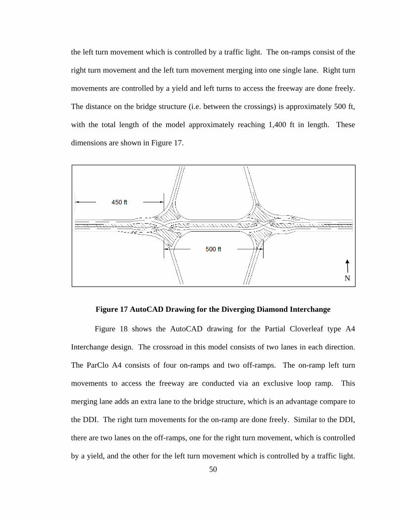
Figure 17 AutoCAD Drawing for the Diverging Diamond Interchange .......................... 50
Figure 18 AutoCAD Drawing for ParClo A4 ................................................................... 51
Figure 19 AutoCAD Drawing for ParClo B4 ................................................................... 52
Figure 20 Diverging Diamond Interchange Conflict Points ............................................. 53
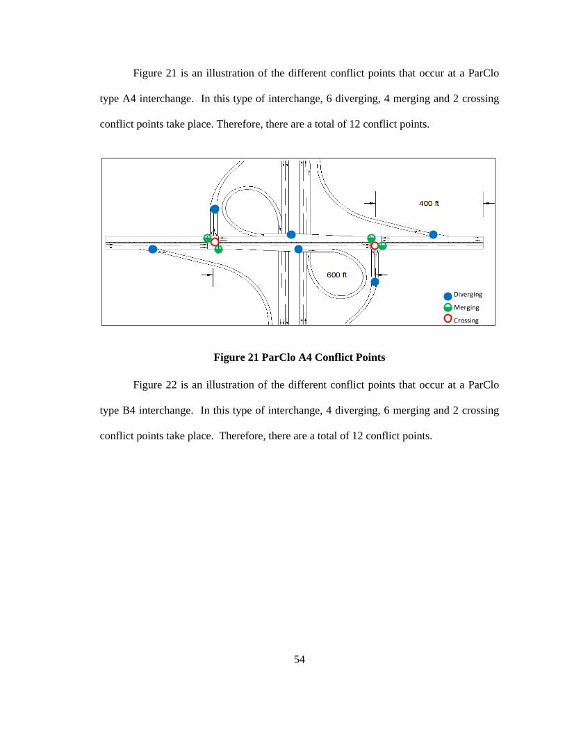
Figure 21 ParClo A4 Conflict Points ................................................................................ 54
Figure 22 ParClo B4 Conflict Points ................................................................................ 55
Figure 23 Synchro’s Optimization Functions (Husch et. al., 2006) ................................. 56
Figure 24 Movements and Phase Numbering Scheme for the DDI .................................. 58
Figure 25 Optimal Signal Timing Plan for DDI 4 High 3.1 Volume Scenario ................ 59
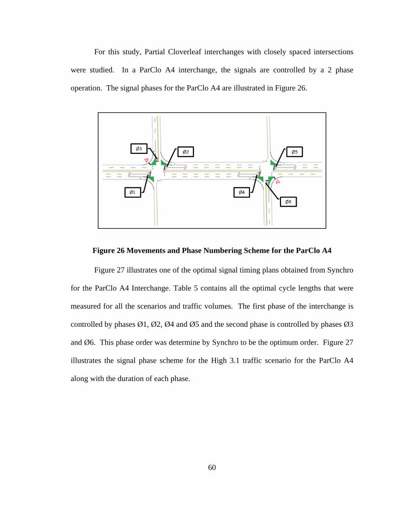
Figure 26 Movements and Phase Numbering Scheme for the ParClo A4 ........................ 60
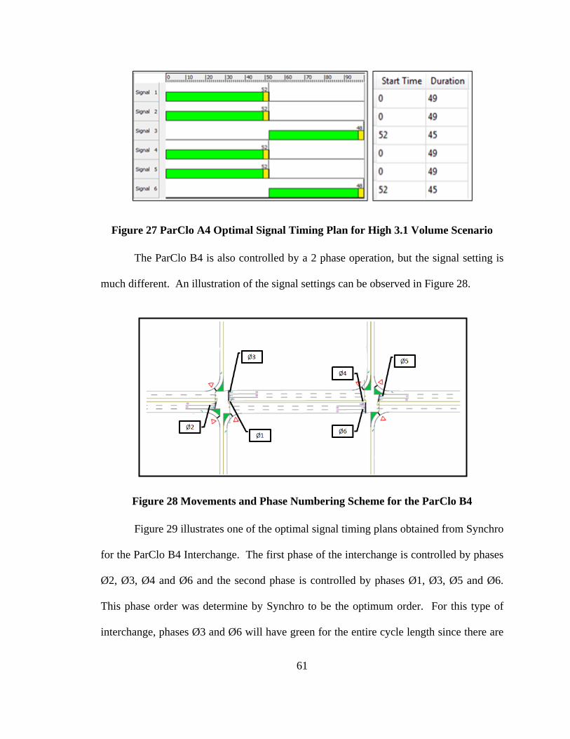
Figure 27 ParClo A4 Optimal Signal Timing Plan for High 3.1 Volume Scenario ......... 61
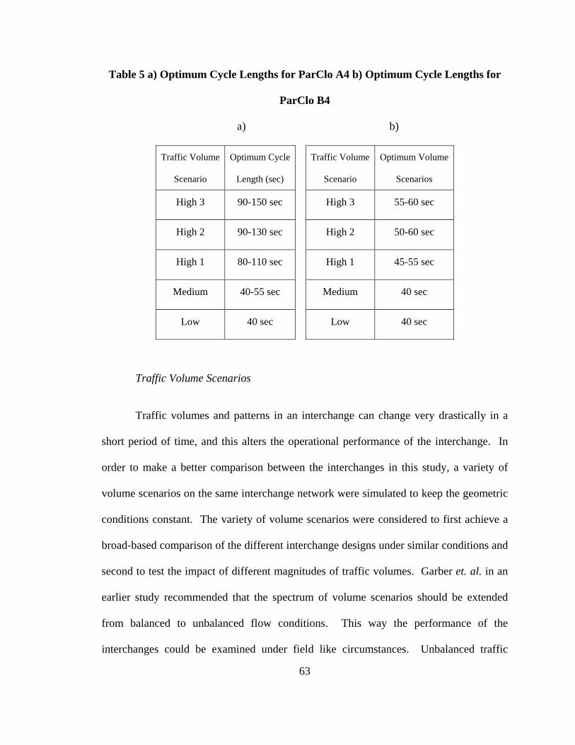
Figure 28 Movements and Phase Numbering Scheme for the ParClo B4 ........................ 61
Figure 29 ParClo B4 Optimal Signal Timing Plan for High 3.1 Volume Scenario .......... 62
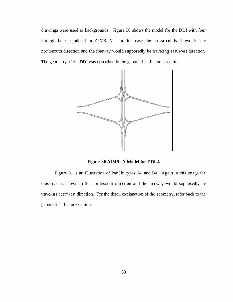
Figure 30 AIMSUN Model for DDI-4 .............................................................................. 68
Figure 31 AIMSUN Models for a) ParClo A4 and b) ParClo B4 ..................................... 69
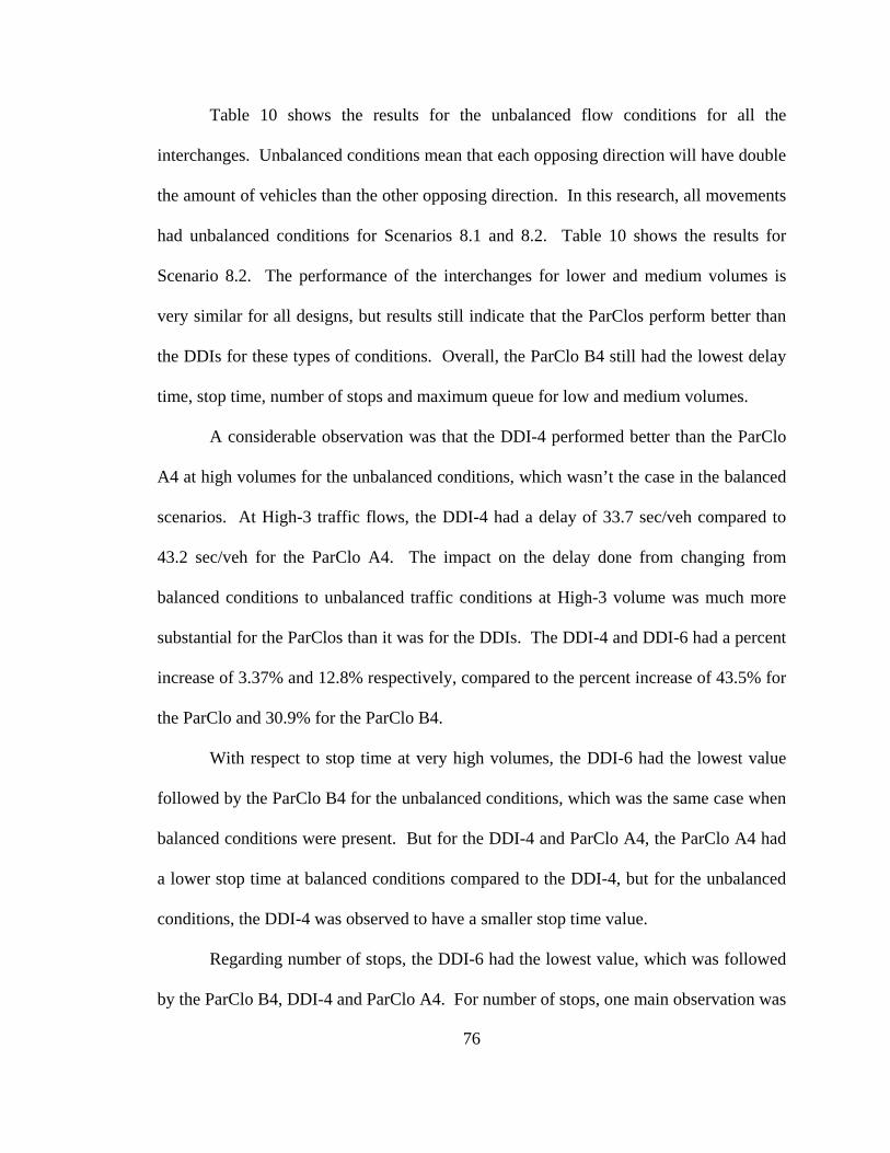
Figure 32 Results for Delay Time for Low and Medium Scenarios ................................. 80
Figure 33 Results for Delay Time for High Scenarios ..................................................... 83
Figure 34 Results for Stop Time for Low and Medium Scenarios ................................... 84
Page 12
xi
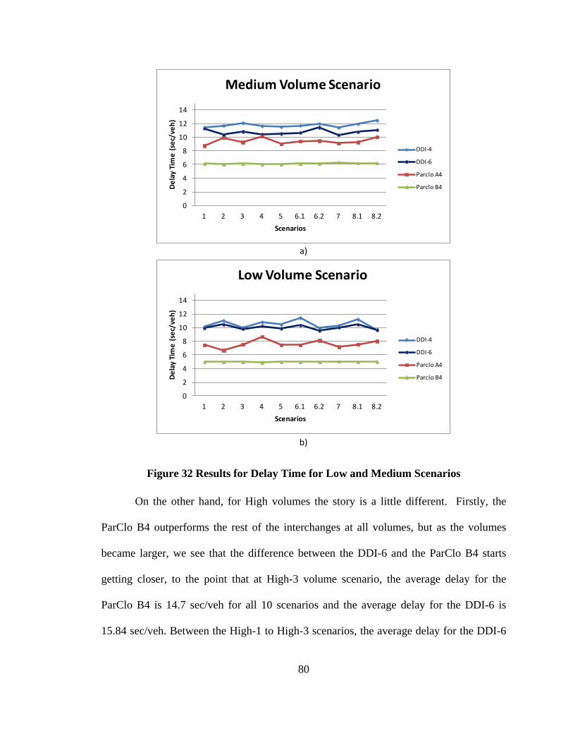
Figure 35 Results for Stop Time for High Scenarios ........................................................ 86
Figure 36 Results for Number of Stops for Low and Medium Scenarios ........................ 87
Figure 37 Results for Number of Stops for High Scenarios ............................................. 90
Figure 38 Results for Maximum Queue Lengths for Low and Medium Scenarios .......... 91
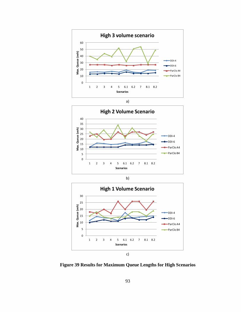
Figure 39 Results for Maximum Queue Lengths for High Scenarios .............................. 93
Page 13
xii
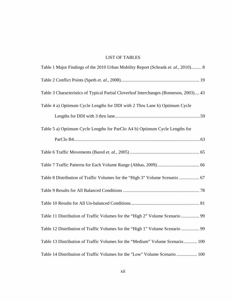
LIST OF TABLES
Table 1 Major Findings of the 2010 Urban Mobility Report (Schrank et. al., 2010) ......... 8
Table 2 Conflict Points (Speth et. al., 2008)..................................................................... 19
Table 3 Characteristics of Typical Partial Cloverleaf Interchanges (Bonneson, 2003) .... 43
Table 4 a) Optimum Cycle Lengths for DDI with 2 Thru Lane b) Optimum Cycle
Lengths for DDI with 3 thru lane ...........................................................................59
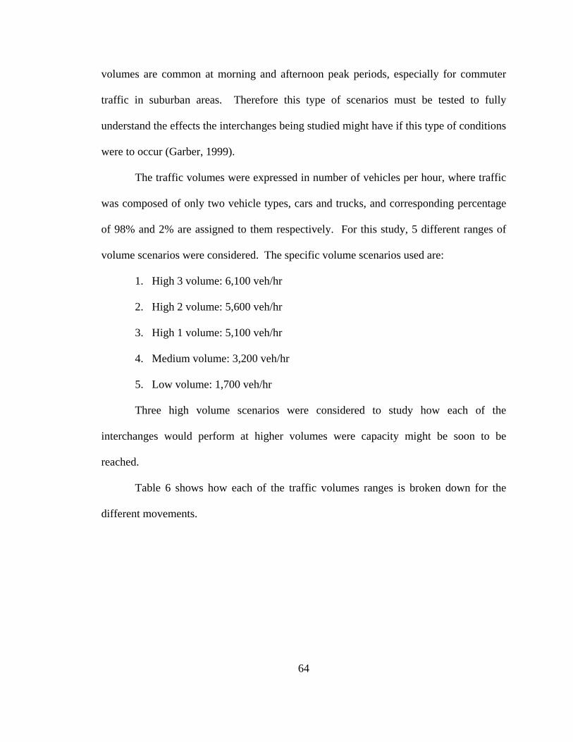
Table 5 a) Optimum Cycle Lengths for ParClo A4 b) Optimum Cycle Lengths for
ParClo B4 ...............................................................................................................63
Table 6 Traffic Movements (Bared et. al., 2005) ............................................................. 65
Table 7 Traffic Patterns for Each Volume Range (Abbas, 2009) ..................................... 66
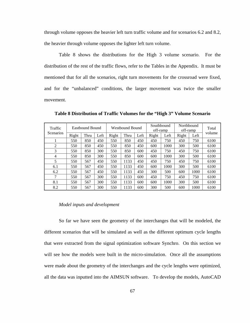
Table 8 Distribution of Traffic Volumes for the “High 3” Volume Scenario .................. 67
Table 9 Results for All Balanced Conditions ................................................................... 78
Table 10 Results for All Un-balanced Conditions ............................................................ 81
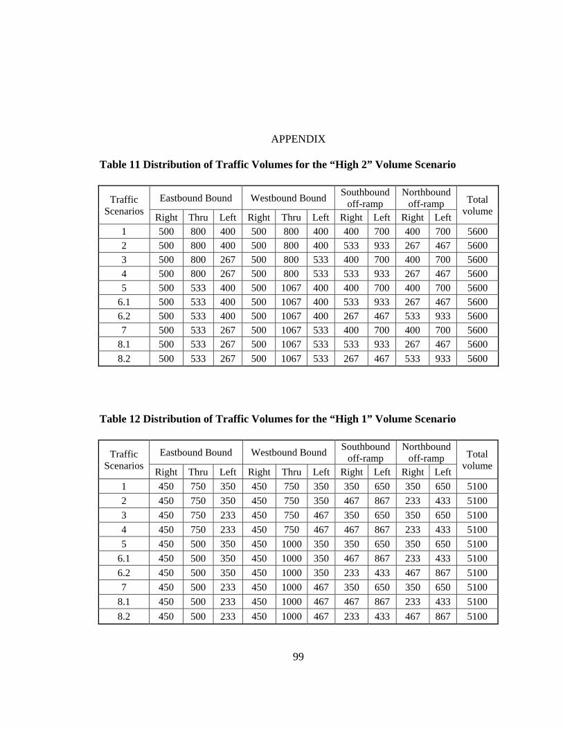
Table 11 Distribution of Traffic Volumes for the “High 2” Volume Scenario ................ 99
Table 12 Distribution of Traffic Volumes for the “High 1” Volume Scenario ................ 99
Table 13 Distribution of Traffic Volumes for the “Medium” Volume Scenario ............ 100
Table 14 Distribution of Traffic Volumes for the "Low" Volume Scenario .................. 100
Page 14
1
INTRODUCTION
The need for innovation in the highway sector has never been greater. The
highway system has had a major impact in the U.S. society and economy, and the
American lifestyle very strongly depends on it. Mobility has become a necessity since
people have grown accustomed to it. Whether driving or riding the bus, many Americans
use the highway system every day in their personal, social or professional activities.
According to the Bureau of Transportation Statistics from 2006, Americans use personal
vehicles for 87 percent of daily trips and 90 percent of long-distance trips (Bureau of
Transportation Statistics, 2006).
Many Nation’s economies are depended on an efficient highway system, whose
functioning would be unimaginable without the access highways provide for motor
vehicles. The U.S. is without exception one of those nations. The 4 million mile
highway system, which serves more than 300 million residents and 7 million business
establishments, carries over 65 percent of the nation’s $15 trillion in freight traffic and 88
percent of all noncommercial person miles traveled (TRB, 2009).
For many years the highway system has been under very severe stress. Most of
the U.S. highways, which have been in constant use for decades, were built to sustain and
accommodate traffic conditions that no longer exit. Over the past decade traffic has
changed not only in numbers but in their nature as well since now we are in the presence
of car that can travel much faster. Most of these highways have exceeded their original
Page 15
2
design life and are now deteriorating and heavily congested (TRB, 2009). So the need
for new innovative designs has never been more important. In the following sections, the
motivation of conducting this work and the different problems that society and
transportation engineers are faced with due to the deterioration of highways and the
increase in congestion will be explained in more detail. Before venturing into the
literature review section, the objectives of this study will be clearly explicated.
Motivation
The United States has always been a very competitive nation in the global
economy. The system of highways, bridges, public transportation, and railroads on
which the nation depends upon have been the main cause of this achievement. The
United States in contrast to the Western world relies more on its roads both for personal
and commercial use. Car ownership is virtually universal excepting few of the larger
cities where mass transit systems have been built. The development of the Interstate
System allowed the U.S. economy in the last half of the 20th century to nourish and grow
in size and productivity. But nowadays the capacity and the performance of the current
Interstate Highway System are too congested and this will reduce the Interstate’s ability
to sustain the increased productivity this country will need to compete in the global
economy.
The introduction of the automobile in the late 19th century signaled the beginning
of an era of mobility in the United States and ended the era of the railroads as the
predominant transportation for people and goods. In the early 20th century, with the
introduction of the national highway system, automobiles were made the number one
Page 16
3
mode of travel for most Americans. The use of private automobiles provided Americans
with a high degree of personal mobility, continuing to allow people to travel where and
with whom they wanted. In the 1950’s the creation of the Eisenhower Interstate
Highway System, composed of high-capacity, high-speed roadways, made available the
connection throughout the United States (Weingroff, 2006).
The transportation system the nation depends upon has largely been built the past
60 years, and much of the system is getting older and needs to be replaced or rebuilt.
One example is the 47,000 mile Interstate Highway System, which represents about 1
percent of the total U.S. road miles, consists of almost 15,000 interchanges, in which
many are wearing out or do not meet current operational standards. Over the years, the
amount of highway mileage built has been substantial, but the raise in travel has been so
great that most of the capacity and reliability when the system was built have been used
up. Travel on the U.S. highway system has increased significantly from 600 billion
vehicles miles traveled (VMT) in 1956 to 3 trillion VMT in 2006 (AASHTO, 2007).
The U.S. is a vast nation which has defeated the tyranny of distance through
investments in a highway system that has connected together and linked communities to
the world. So far, the highway system has provided American consumers and businesses
with an unparalleled mobility and choice. Today Americans conduct over 90 percent of
U.S. trips to work and 88 percent of all those trips are made by automobiles (Rodrigue et.
al. 2009). The invention and the vast acceptance of the automobiles have allowed people
to travel where they want, when they want and with whom they want. Demand mobility,
comfort, status, speed and convenience are some of the obvious advantages related to
automobile use. Thus, automobile ownership continues to grow worldwide, which is an
Page 17
4
illustration of these advantages. Most individuals, when given the choice and the
opportunity, will favor the use of an automobile. One of the main problems of the growth
in the total number of vehicles is that it gives rise to congestion at peak traffic hours on
all road systems (AASHTO, 2007).
During the construction of the Interstate Highway System in the 1950s, the
economy of the United States was mainly self-contained. But at the moment this has
changed, since the percentage of U.S. Gross Domestic Product (GDP) represented by
foreign trade increased from 13 percent in 1990 to 26 percent in 2000 and is expected to
reach 35 percent by 2020. Consequently, the number of containers moving through U.S.
ports has increase from 8 million units in 1980 to over 40 million in 2006 and is expected
to arrive at 110 million by 2020. To carry those containers as well as the growing
domestic traffic, truck freight on our highways is expected to increase over 100 percent
by 2035. Highways are the basis of the U.S. freight transportation system carrying nearly
80 percent of domestic tonnage and 94 percent domestic value. Trucks have provided
direct service for both long-distance and local shipments, and provide the pickup and
delivery for long-distance shipments made by rail or overnight airfreight. So an efficient
highway system is necessary to maintain the economical stability this nation has
experienced in the last decades (AASHTO, 2007).
Over the next 50 years, forecasts have indicated that the U.S. population will
grow from 300 million to 435 million. The amount of increase expected will be about an
equivalent of another Canada to be added each decade. So the main question is what
needs to be done so that the Highway System of the future can continue to play its role as
Page 18
5
a strategic national highway network, with the capacity to move all the freight and
automobiles traffic with an adequate speed and reliability (AASHTO, 2007).
Problem Statement
Some of the main industries in the United States are travel, tourism and
recreation. Together they rank as the top three industries in all the states. In contrary to
extractive industries, such as timber and mining, which have been declining in many
parts of America, the role of travel, tourism and recreation has been in a climb. This
industry, which generated over $700 billion in revenues in 2007, directly depends on a
good transportation system (AASHTO, 2007).
In the United States travel is measured in vehicle miles traveled (VMT), and since
1955 to 2006, travel has increase from 600 billion to 3 trillion VMT per year. U.S.
DOT’s 2004 Conditions and Performance estimated that this amount will grow by 2.07
percent through 2022, and at this rate by 2055, VMT is expected to exceed 7 trillion.
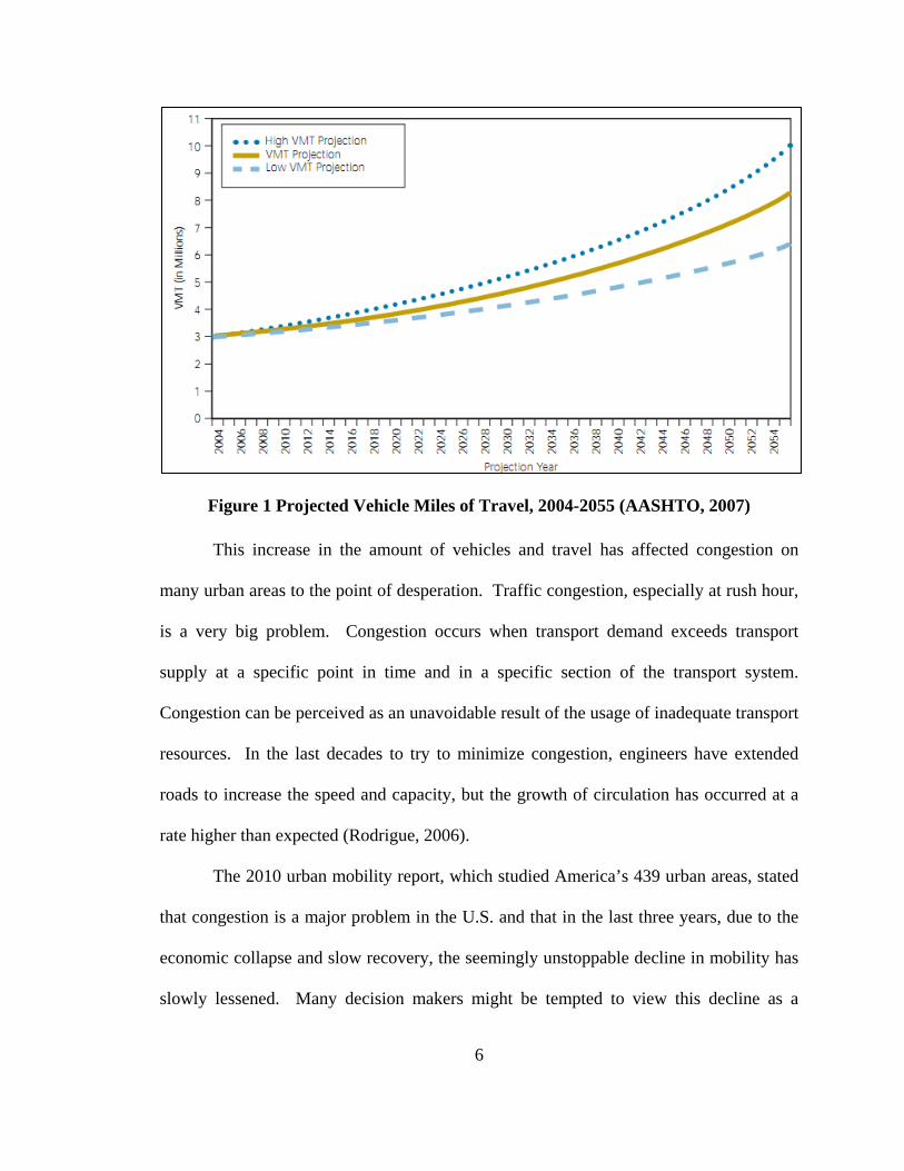
This expected increase is illustrated in Figure 1. The number of licensed drivers has also
grown from 78 million approximately 50 years ago to 205 million today and is expected
to grow over 380 million 50 years from now. These days, highways carry over 246
million vehicles compared to 65 million vehicles in 1956, and the amount of vehicles is
expected to reach nearly 400 million by 2055 (AASHTO, 2007).
Page 19
6
Figure 1 Projected Vehicle Miles of Travel, 2004-2055 (AASHTO, 2007)
This increase in the amount of vehicles and travel has affected congestion on
many urban areas to the point of desperation. Traffic congestion, especially at rush hour,
is a very big problem. Congestion occurs when transport demand exceeds transport
supply at a specific point in time and in a specific section of the transport system.
Congestion can be perceived as an unavoidable result of the usage of inadequate transport
resources. In the last decades to try to minimize congestion, engineers have extended
roads to increase the speed and capacity, but the growth of circulation has occurred at a
rate higher than expected (Rodrigue, 2006).
The 2010 urban mobility report, which studied America’s 439 urban areas, stated
that congestion is a major problem in the U.S. and that in the last three years, due to the
economic collapse and slow recovery, the seemingly unstoppable decline in mobility has
slowly lessened. Many decision makers might be tempted to view this decline as a
Page 20
7
change in trend or a sign that the congestion problem is slowly been solved, however the
data from the 2010 Urban Mobility Report does not support this conclusion since the
problem is larger than expected and also since history has shown that after a recession,
traffic growth comes roaring back (Schrank et. al., 2010).
In 2009, congestion caused urban Americans to travel 4.8 billion hours more and
to purchase an extra 3.9 billion gallons of fuel adding up to a total cost of $115 billion,
and all this waste comes with a heavy price in terms of wasted productivity and fuel.
2008 appeared to be the best year for congestion in recent times since congestion
worsened in 2009. But this is no reason for celebration since prior to the economy
slowing, just 5-6 years ago, congestion levels were much higher than a decade ago, and
these conditions are expected to return with a strengthening economy (Schrank et. al.
2010). Table 1 shows the major findings of the 2010 Urban Mobility Report. An
important detail to mention is that the delay, the travel time and the fuel wasted compared
to 2007 have gone down for individuals as well as for the entire nation, but these values
are still very high and they has been forecasted to increase in the future.
Page 21
8
Table 1 Major Findings of the 2010 Urban Mobility Report (Schrank et. al., 2010)
It is known that during the past decade, highway congestion levels have steadily
worsened as our nation’s population and need for travel have grown at a higher rate than
the infrastructure’s capacity. It is also known that congestion not only negatively affects
travel, but it also affects business efficiencies, energy availability and air quality, and If
not treated, congestion will have a great impact in the recovery of the nation’s
economical growth. According to the U.S. Department of Transportation’s Bureau of
Transportation Statistics, transportation has a vital importance to the U.S. economy since
more than $1 out of every $10 produced in the U.S. gross domestic product is related to
transportation activity (Bureau of Transportation Statistics, 2006).
The consequence of all the increase in population the increase in the amount of
cars has been the main reason why highways and road systems do not have the capacity
to handle the vehicle load during peak-hour without forcing many people to wait in line.
Page 22
9
Studies have forecasted that the amount of traffic in the future is expected to grow, and if
some measures are not taken, the nations’ economy might be in big danger.
Overview of Approach
Congestion has cost this country $115 billion for the 2009 year in delays and
wasted fuels, and there doesn’t seem to be one solution that will fix this problem
(Schrank et. al. 2010). There have been many solutions recommended to decrease the
congestion such as the usage of public transportation, carpooling, asking businesses to
help reduce travel peak hours by letting employees work earlier or late shifts, or
increasing efficiency and adding capacity to the existing roads and transit systems.
But the fact is that demand for highway travel by Americans will continue to
grow as population increases. Rising traffic congestion is an inescapable condition, and
the peak hour traffic congestion is a natural result of the way modern societies operates.
Traffic congestion has primarily been the result of the basic mobility problem, which is
that too many people want to move at the same times of the day. In the current society,
efficient operations require that people work and run errands at about the same time so
that they can interact with each other. So this basic requirement cannot be altered
without having a great impact in the economy and society of the United States (Downs,
2004). The vast majority of people seeking to move during rush hours use private
vehicles for one main reason, which is that privately owned vehicles are faster, more
private, more comfortable, more convenient in trip timing, and more flexible for doing
multiple tasks on one trip. With almost 88 percent of American’s daily commuters using
private vehicles, and millions more wanting to move at the same time of days,
Page 23
10
American’s problem is that its highways and road systems do not have the capacity to
handle the vehicle load during peak-hour without forcing many people to wait in line
(Downs, 2004).
The roadway infrastructure has been pushed to its limit due to the gradual rise of
travel demand. Mobility in the U.S. is considered a major necessity, but today’s traffic
engineers and planners are challenged with a major problem, which is to meet these
mobility needs with very little resources while population growth escalates faster than
infrastructural growth. Over the years, engineers have come up with different solutions
to minimize congestion. One solution to alleviate congestion is the invention of new
innovative designs that can optimize the performance of roadway systems.
For many years, one of the main focus and concerns of transportation
improvements have been physical bottlenecks. Highway systems are notorious for
causing congestion on very specific points. One of these locations that has proven to
cause a lot of congestion on a daily basis are interchanges, and how bad congestion
becomes is mainly related to the physical design of these structures. Many of these
interchanges were originally constructed many years ago when the designs were
appropriate for the conditions present then, but are now considered outdated since they do
not perform according to the flow of traffic present (FHWA, 2005).
The interstate system, which has been one of the main sources of this countries
economical success, consists of around 15,000 interchanges for which many of them do
not meet current operational standards. Most of the significant congestion occurring at
the interstate system takes place at interchanges because they were not designed to carry
the volume of traffic that currently uses them. This blockage point, where most of the
Page 24
11
congestion occurs, creates many holdups and safety problems and the projected future
traffic volumes will make these problems much worse. The main goal of any well
designed interchange is to sustaining traffic flowing smoothly, but with congestion
worsening, new measures will need to be implemented so that these interchanges can
work efficiently (AASHTO, 2007).
After the implementation of the interstate highway system, the use of interchanges
became more prevalent to improve the flow on the nation’s new highways (Garber et. al.,
1999). Originally, to select an interchange type, the engineers would solely base the
selection in the site’s physical limitations and the forecasted traffic volumes. During the
1870s and 1980s, new and improved knowledge of traffic flow theory and better human
factors research caused an improvement of the interchange selection process (Garber et.
al., 1999). As a result of these new knowledge’s, there was a comprehension that factors
such as access control, highway classification, design speed, traffic composition,
construction costs, right-of-way issues, and safety needed to be considered in the
selection of the interchange. Despite all the progress in the interchange selection
methods, there are still a number of interchanges nationwide that are either under or over
designed (Garber et. al., 1999).
As defined by the AASHTO “Green Book” an interchange is a system of
interconnecting roads in conjunction with one or more grade separations that provide
movement of traffic between two or more roadways or highways on different levels
(AASHTO, 2004). The most distinguished features of any interchange are ramps, which
permit connection and access between intersecting roadways. Throughout the years,
interchanges have come in a diverse array of geometry forms with a range of design
Page 25
12
features. Grade separations have been in use to improve traffic flow since the first
development of the interchange in 1928 (Garber et. al., 1999).
Interchanges can vary from single ramps connecting local streets to complex
design layouts involving multiple highways. There are many basic interchange
configurations which are indicated in the Exhibit 10-1 in Chapter 10 in the 2004
AASHTO Green Book (AASHTO, 2004). The decision for the application of a type of
interchange configuration is based on many variables such as the number of intersection
legs, surrounding topography and culture, the degree of flexibility in the traffic operations
desired, type of truck traffic, right-of-way and practical aspects of costs among others.
Signing and operations are also major considerations in the design and implementation of
an interchange (PennDOT, 2009). Understanding which type and form of interchange are
best for a given location and a given purpose is the job of the transportation engineer.
The basic interchange types can be classified in terms to include three-leg
designs, four-leg designs and other special interchange designs involving two or more
structures. Three-leg designs represent an interchange with three intersecting legs
consisting of one or more highway grade separations and one-way roadways for all traffic
movements. Examples of three-leg designs, which are also designated as T or Y
interchanges, include the trumpet interchange, directional T type interchange and a fully
directional interchange (MaineDOT, 2004). Four-leg designs represent interchanges with
four intersection legs which may be grouped under six general configurations. The four-
leg designs can be classified as Diamond Interchanges, Single-Point Urban Interchanges
(SPUIs), Partial Cloverleafs, Full Cloverleaf and Interchanges with direct and semidirect
connections (PennDOT, 2009). In addition to interchange types, different definitions
Page 26
13
apply to interchange designations. “System interchanges” are interchanges between two
fully access-controlled highways or freeway. On the other hand, “service interchanges”
are interchanges where one or both of the intersecting highways are not a fully access-
controlled facility (e.g. arterial roads) (MaineDOT, 2004).
To sustain all this growth in vehicles and travel, engineers will need to come up
with new innovative interchange designs that can minimize congestion and delays
allowing the traffic to move smoothly so that the economy of this nation can keep on
growing. One such innovative design is the Diverging Diamond Interchange (DDI). One
of the main goals of the DDI interchange design is to accommodate left-turn movements
and hence eliminate a phase in the signal cycle (Sharma et. al., 2007). This design has
been in use since 2009 and has been studied and compared to many other interchanges.
The outcome of all these studies has been very promising, and they have shown that the
DDI interchange can increase flow, decrease congestion and allow for a heavy left turn
movement. Another interchange that is known to allow for heavy left turn movement is
the Partial Cloverleaf. In contrast to the DDI, the Partial Cloverleafs have been in use for
many decades now and consists of 16% of all the types of interchanges in the U.S.
(Bonneson, 2003). Therefore in this study, the DDI will be compared to the Partial
Cloverleaf Interchange type A4 and B4 because of their similarities to: allow for more
left turn movements, having ramps in all quadrants and been controlled by a two phase
operation.
Page 27
14
LITERATURE REVIEW
The primary goal of this research is to evaluate and compare the operational
performance of several interchanges, which include a Diverging Diamond Interchange
and the different types of Partial Cloverleaf, using a micro simulation platform. The
results of this comparison will assist decision makers in selecting and determining which
design will be the most appropriate for particular locations A thorough literature review,
focusing on the characteristics and potential benefits and drawbacks of each interchange,
the procedures for analyzing interchanges, a review of available simulation platforms, as
well as results from previous studies, was performed in order to attain the goal of this
research.
Diverging Diamond Interchange
Chlewicki (2003) introduced two new designs developed by himself, the
Synchronized Split-Phasing Intersection and the Diverging Diamond Interchange (DDI).
The designs take advantage of the benefits of split-phasing and signal synchronization to
theoretically improve signal timing at heavy volume interchanges or heavy turning
movements. Simulations were conducted to compare the delay and total stops of these
new designs to other conventional designs. The idea behind the DDI was to use the
crossing over movement on an interchange design. The conventional diamond
interchange seemed to be the easiest design to create crossover movements for. The main
Page 28
15
goal was to better accommodate left turn movements and potentially eliminate a phase in
the cycle for the signals. Figure 2 shows the layout of the diverging diamond
interchange. The highway portion, shown in the northbound/southbound direction, does
not change but the movements off the ramps change for left turns. Through and left turn
traffic for the arterial road also maneuvers in a different manner from a conventional
diamond interchange because the traffic crosses to the “wrong” side in between the
ramps.
Figure 2 Diverging Diamond Interchange (Chlewicki, 2003)
The biggest potential benefit for the DDI is the ability to combine phases in ways
that cannot be done in other interchange designs. Ramp phases can be combined with a
mainline through movement, and mainline left movements can be combined with though
movement throughout the whole phase. Also coordination of the signals can be made
between a ramp phase and a through phase without much difficulty and the reduction of a
phase could benefit the signal timing. Also the diverging diamond interchange was found
to have less conflict points than a conventional diamond interchange. The diverging
Page 29
16
diamond interchange was compared to a standard diamond interchange, where the total
delay for the conventional diamond was about three times as great as the diverging
diamond, and the stop delay was over four times. The authors stated there seemed to be
great potential for the DDI design but more research would be needed to be done to look
into alterations in traffic patterns and signal spacing, as well as a cost analysis.
Bared et. al., (2005) presented the results of a study on two new alternative
designs, one of them being the Diverging Diamond Interchange. This design was studied
for different traffic scenarios using traffic simulation and the results showed better
performance including level of service, delay, queue, and throughput during peak hours
when compared to similar corresponding conventional designs. Two different designs of
DDI are analyzed which are a four-lane DDI, in which the total number of lanes is 4 in
the arterial road, and a six-lane DDI in which the total number of lanes is six in the
arterial road. For the four-lane DDI, five different traffic flow scenarios were considered
which included one low, one medium, and three high flows (to measure the performance
beyond the capacity of the conventional diamond). For the six-lane DDI, six traffic flow
scenarios were considered which consisted of one low, one medium and four high flows.
The geometry proposed to model the DDI by Bared is shown in Figure 3.
Page 30
17
Figure 3 Layout of a Diverging Diamond Interchange Design (Bared et. al., 2005)
The signal phasing scheme that was proposed for the DDI is shown in Figure 4.
For this signal scheme, a cycle length of 70 second was found to be optimal for lower to
medium flows, and a cycle length of 100 seconds was found best for higher flows. The
amber time used was 3 sec. and the all-red period was 2 sec at the end of every phase.
The signal was set to operate under two phases.
Page 31
18
Figure 4 Signal Settings for a DDI (Bared et. al., 2005)
The conclusions extracted by these study was that for higher traffic volumes, the
DDI has better performance and offers lower delays, lesser number of stops, lower stop
time and shorter queue lengths as compared to the performance of the conventional
design. For lower volumes, the performance of DDI and conventional intersection were
similar. The capacity for all signalized movements was higher for the DDI as compared
to the conventional diamond. Also while the DDI does now allow trough movements
from off- to on-ramps, it allows u-turn movements with fewer conflicts than at a
conventional diamond interchange.
Page 32
19
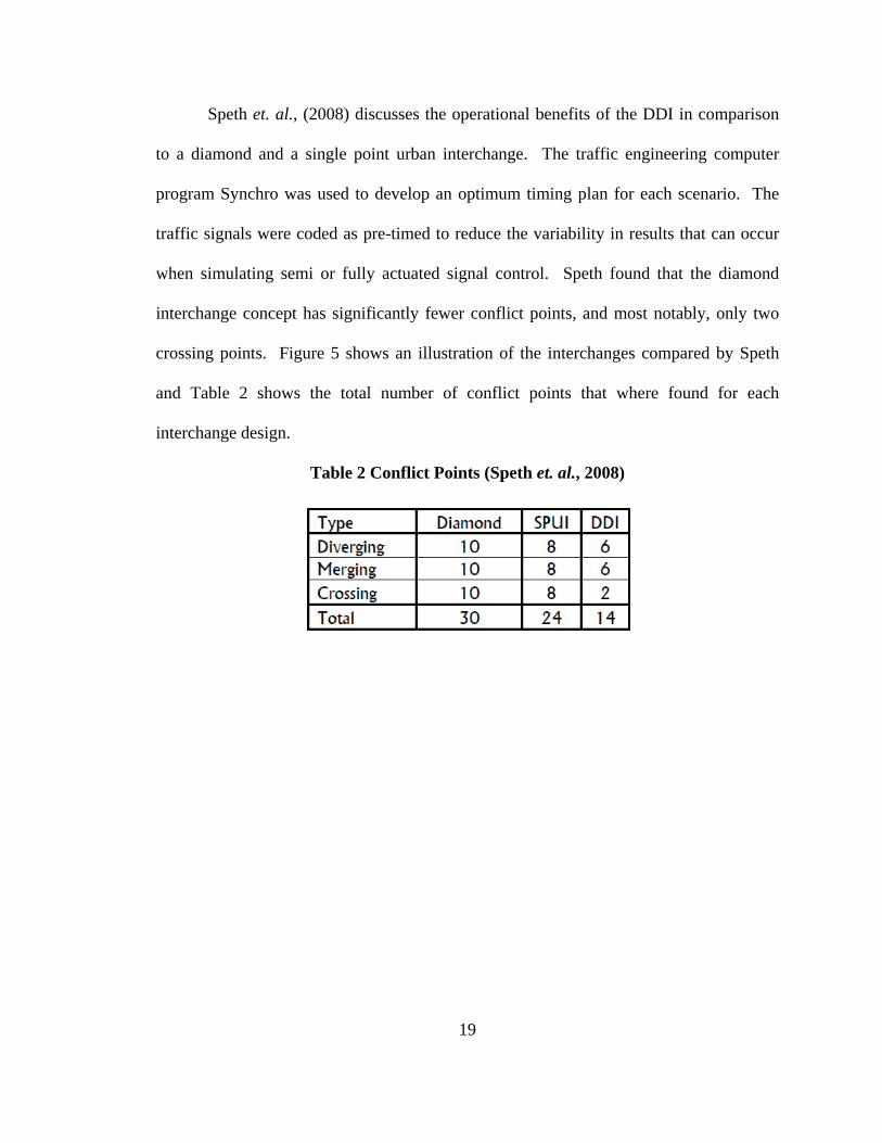
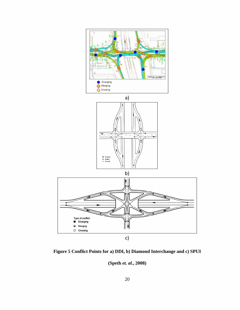
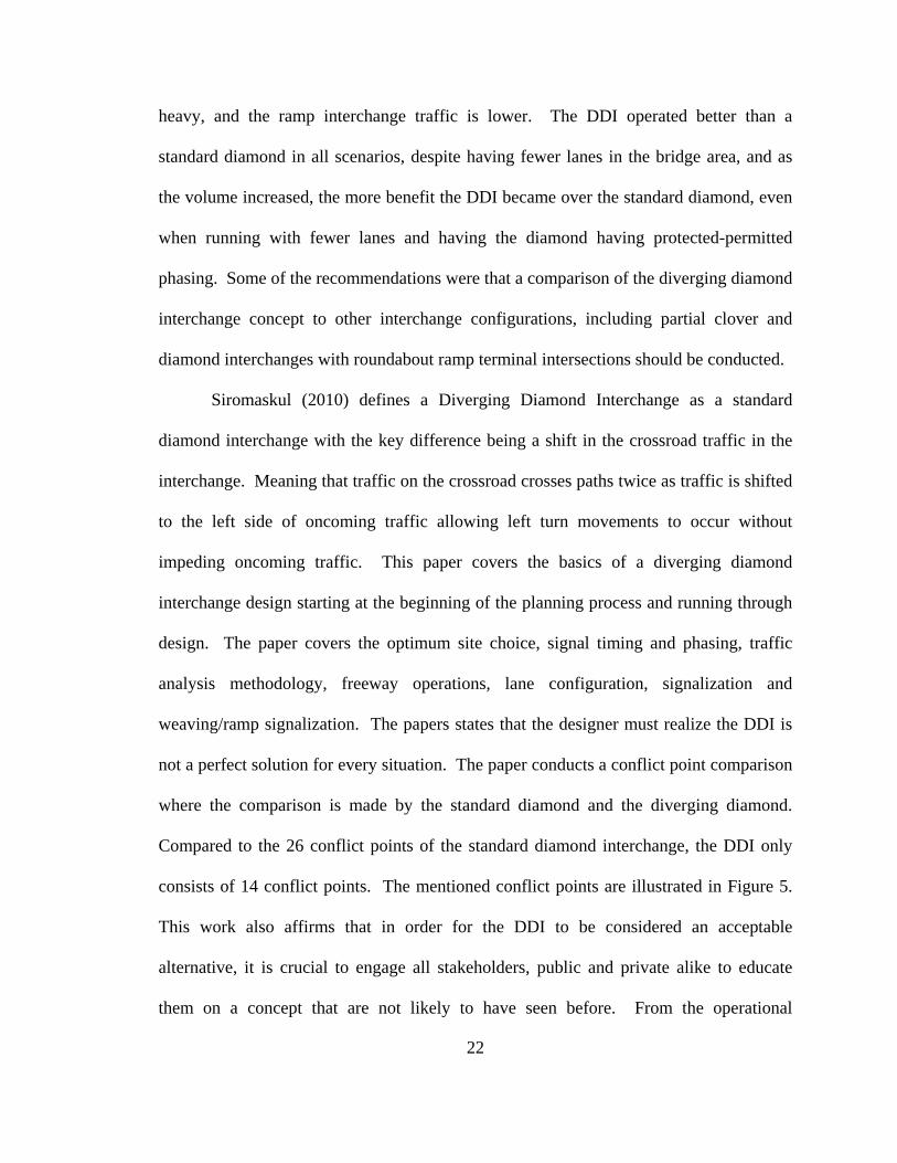
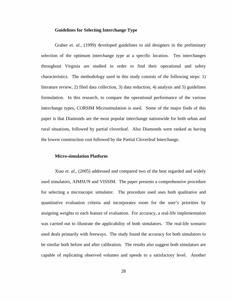
Speth et. al., (2008) discusses the operational benefits of the DDI in comparison
to a diamond and a single point urban interchange. The traffic engineering computer
program Synchro was used to develop an optimum timing plan for each scenario. The
traffic signals were coded as pre-timed to reduce the variability in results that can occur
when simulating semi or fully actuated signal control. Speth found that the diamond
interchange concept has significantly fewer conflict points, and most notably, only two
crossing points. Figure 5 shows an illustration of the interchanges compared by Speth
and Table 2 shows the total number of conflict points that where found for each
interchange design.
Table 2 Conflict Points (Speth et. al., 2008)
Page 33
20
a)
b)
c)
Figure 5 Conflict Points for a) DDI, b) Diamond Interchange and c) SPUI
(Speth et. al., 2008)
Page 34
21
Speth noted that the number of simultaneous points of conflict, which do not exist
in the diverging diamond interchange concept, as any vehicle entering the intersections
can only be struck one direction. The paper stated that the conflict points of a DDI
require significantly less yellow and all red time to control, which in turn give less lost
time and more green time and more capacity. In this study, the traffic operations of the
three interchange designs were compared for four different volume scenarios in order to
get a good understanding of the conditions that affect each of the interchange types. To
compare the capacity and delay characteristics of the interchange types, the traffic
patterns were varied with high balanced ramp volumes, high unbalanced ramp volumes,
heavy arterial volumes, mid-to heavy level overall volumes, and a real-world projected
condition shown as volume scenarios in Figure 6.
Figure 6 Traffic Volumes (Speth et. al., 2008)
The results of this study by Speth concluded that the DDI configuration increases
in value of different MOEs with more volume, especially with the increase of ramp
volume. The least beneficial scenario was found to be when the arterial volumes are
Page 35
22
heavy, and the ramp interchange traffic is lower. The DDI operated better than a
standard diamond in all scenarios, despite having fewer lanes in the bridge area, and as
the volume increased, the more benefit the DDI became over the standard diamond, even
when running with fewer lanes and having the diamond having protected-permitted
phasing. Some of the recommendations were that a comparison of the diverging diamond
interchange concept to other interchange configurations, including partial clover and
diamond interchanges with roundabout ramp terminal intersections should be conducted.
Siromaskul (2010) defines a Diverging Diamond Interchange as a standard
diamond interchange with the key difference being a shift in the crossroad traffic in the
interchange. Meaning that traffic on the crossroad crosses paths twice as traffic is shifted
to the left side of oncoming traffic allowing left turn movements to occur without
impeding oncoming traffic. This paper covers the basics of a diverging diamond
interchange design starting at the beginning of the planning process and running through
design. The paper covers the optimum site choice, signal timing and phasing, traffic
analysis methodology, freeway operations, lane configuration, signalization and
weaving/ramp signalization. The papers states that the designer must realize the DDI is
not a perfect solution for every situation. The paper conducts a conflict point comparison
where the comparison is made by the standard diamond and the diverging diamond.
Compared to the 26 conflict points of the standard diamond interchange, the DDI only
consists of 14 conflict points. The mentioned conflict points are illustrated in Figure 5.
This work also affirms that in order for the DDI to be considered an acceptable
alternative, it is crucial to engage all stakeholders, public and private alike to educate
them on a concept that are not likely to have seen before. From the operational
Page 36
23
comparison, it was determined that the DDI’s effectiveness at managing traffic increases
as the turning volume increases. One of the major benefits to a DDI occurs in the
decrease in the number of lanes required to manage the same traffic that other concepts
may require several additional lanes and multiple turn lanes to manage. Also it is found
that the DDI decreases the impact of merging vehicles on the traffic on the freeway as
merging traffic is not as heavy platooned as it reaches the freeway mainline.
Chlewicki (2010) introduced a paper with theories on how the DDI works by
examining the signal progressions both within the interchange and outside of the
interchange. Chlewicki examined the unique traffic pattern within the interchange to
make the interchange more effective. He also examines the unique traffic pattern that is
established beyond the interchange at subsequent signals to increase the overall
efficiency of the traffic progression for the entire corridor. This research determined that
several factors play into synchronizing any two signals in the DDI, which are the space
between signals, the speed of the vehicles, the cycle lengths, and the phase distribution.
The procedure suggested by this research in designing a DDI was to (1) Lay out a rough
schematic of DDI, (2) Determine cycle splits at each signal in the interchange for the
design year during peak periods, (3) Determine the basic synchronization strategy based
on turning movement volumes and consider the cycle length needs, (4) Determine how
much time would be ideal to get from the first signal to the second signal, (5) Adjust
speed and the distance between the crossover signals to optimize synchronization, (6)
Make slight adjustments as necessary to signal timing to maximize the optimization, (7)
Lay out signal along the corridor adjacent to the DDI and re-examine the cycle lengths
based on the whole system and (8) Make adjustments as needed. Chlewicki states that
Page 37
24
determining the correct cycle length can significantly increase the amount of bandwidth
in both direction of the progression and that taking the signal timing into consideration
during design can make an effective design even better.
Sharma et. al. (2007) presented a paper of the results of a study comparing the
Diverging Diamond Interchange (DDI) to the Conventional Diamond Interchange (CDI).
Both alternatives were studied for a range of volume scenarios using traffic micro
simulation and a cost-effectiveness analysis was also conducted. The results suggested
that for all traffic scenarios the performance of the DDI was found to be better than the
CDI with lower delays for critical movements, lower travel time and lower maximum
queue lengths. It was also found that the DDI showed increased capacity for the critical
movements, particularly for left-turns. Also according to the results found in this
research, a 4 lane DDI would be a superior option to building a 6 lane CDI.
A paper by Abbas et. al. (2009) offered a traffic comparison between the single
point (SPI) and the Diverging Diamond (DDI) grade separated interchanges. The
comparison was conducted by using the VISSIM simulation platform and the MOEs
considered were throughput, delay and number of stops. The analysis was only
conducted for the surface street crossing and ramps, excluding the traffic operations of
the freeway itself. In this research a wide variety of hypothetical traffic flow scenarios
were studied for each design. The results suggested that for balanced conditions the
capacity for the SPI was superior to the DDI. For unbalanced conditions, the sum of
critical lane volume for the DDI was found to gradually increase to a level comparable to
the SPI. When the imbalanced of the crossroad opposing volumes was 30-70% and
greater, the DDI outperformed the SPI. This research also found that the DDI had shorter
Page 38
25
delays than the SPI but the SPI generated fewer number of stops compared to the DDI
design.
Partial Cloverleaf
Milan et. al., (1999) describes the results of a comparison of the traffic operations
of an existing full cloverleaf interchange with the partial cloverleaf interchange
configuration. This work described a case study, conducted on the interchange located
on Sunrise Boulevard/U.S Highway 50 in Sacramento, California, where an evaluation
was conducted to determine if it was necessary to replace the existing full cloverleaf
interchange with a partial cloverleaf configuration to improve peak hour traffic
operations. For the analysis, CORSIM Microsimulation was used as the key analysis
tool. The key findings of this report were that the partial cloverleaf design
accommodates more traffic than the full cloverleaf configuration and also improved the
ability to control off-ramp and arterial traffic flows. The key MOEs that were considered
for the analysis include Total Trips Served, Average Travel Speed, Vehicle Miles
Traveled, Vehicles Hours of Delay and Maximum Queue Lengths for on and off ramps.
Zhang et. al., (2010) studied the possibility of controlling two adjacent T-
intersections and partial cloverleaf interchanges with one controller. The paper described
how a Partial Cloverleaf interchanges has a similar geometry as a dual T-intersection and
therefore the signal timing could basically be the same as the dual T-intersection. The
paper describes six common types of partial cloverleaf interchange which are shown in
Figure 7.
Page 39
26
Figure 7 Six Common Types of ParClos (Zhang et. al., 2010)
It is stated in the paper that generally one controller is adequate to control closely
spaced intersections of interchanges. For diamond interchanges, it is generally
recognized that for intersection spacing less than 800 feet, a single controller should be
used, and for intersections spacing more than 800 feet, two controllers with interconnect
should be provided. The phase scheme using one controller for Parclo A2, B2 and AB2
types are given in Figure 8.
Page 40
27
a)
b)
Figure 8 Phasing Scheme for ParClo a) Types A and b) Type B (Zhang et. al., 2010)
The partial cloverleaf interchanges with four quadrants do not have left-turns
from the off-ramps, and therefore one controller is also adequate to control two
intersections. The signal phasing is firstly given with different phase sequences and
control types. The key findings of this paper were that when closely spaced one
controller can be used in a partial cloverleaf interchange and that the selection of different
phasing scheme can yield to different progression performances.
Page 41
28
Guidelines for Selecting Interchange Type
Graber et. al., (1999) developed guidelines to aid designers in the preliminary
selection of the optimum interchange type at a specific location. Ten interchanges
throughout Virginia are studied in order to find their operational and safety
characteristics. The methodology used in this study consists of the following steps: 1)
literature review, 2) filed data collection, 3) data reduction, 4) analysis and 5) guidelines
formulation. In this research, to compare the operational performance of the various
interchange types, CORSIM Microsimulation is used. Some of the major finds of this
paper is that Diamonds are the most popular interchange nationwide for both urban and
rural situations, followed by partial cloverleaf. Also Diamonds were ranked as having
the lowest construction cost followed by the Partial Cloverleaf Interchange.
Micro-simulation Platform
Xiao et. al., (2005) addressed and compared two of the best regarded and widely
used simulators, AIMSUN and VISSIM. The paper presents a comprehensive procedure
for selecting a microscopic simulator. The procedure used uses both qualitative and
quantitative evaluation criteria and incorporates room for the user’s priorities by
assigning weights to each feature of evaluation. For accuracy, a real-life implementation
was carried out to illustrate the applicability of both simulators. The real-life scenario
used deals primarily with freeways. The study found the accuracy for both simulators to
be similar both before and after calibration. The results also suggest both simulators are
capable of replicating observed volumes and speeds to a satisfactory level. Another
Page 42
29
finding was that most of the standard traffic modeling requirements can be modeled with
both simulators. The main contribution from this paper is that different users have
different preferences but overall these two simulators only have very minor differences in
the features and accuracy. The selection of the best simulator is highly subjective since
AIMSUN and VISSIM simulators are the best ones available.
Page 43
30
METHODOLOGY
The objective of this research is to provide better guidance on one unconventional
design which is the Diverging Diamond Interchange compared to the Partial Cloverleaf
Interchange design which is a conventional interchange design. Therefore, different steps
need to be taken to assure a fair comparison occurs. The first part of the methodology
section introduces the Diverging Diamond Interchange (DDI) and the Partial Cloverleaf
(ParClo) interchanges. This section describes the different characteristics such the
number of ramps as well as the typical geometry for each design. The second part of the
methodology describes the type of micro-simulation to be used to compare the different
interchange designs. The micro-simulation software chosen is described in detail, and the
reason why this particular software was used compared to others is also mentioned. In
this section the different measures of effectiveness extracted from micro-simulation are
defined to understand what measures will be used to conduct the comparison.
The type of interchange configuration used at a specific location is based on a
variety of factors such a highway classification, traffic volume and distribution, design
speed, availability of right of way, degree of access control (Garber et. al., 1999).
Therefore, the next section of the methodology will be dealing with the experimental
design of each interchange. In this section, the geometrical features of each design to be
modeled in micro-simulation will be describes along with the different magnitudes of
traffic volumes and distribution. The next step will be to optimize cycle lengths of each
Page 44
31
interchange for each different scenario by the use of a signal optimization tool. This step
will allow the user to extract the best results for each design so that a fair comparison can
be conducted. Once the required input data is described, the next step will be to use
micro-simulation to obtain results for the different magnitudes of traffic volumes and
distribution tested in this study. Different replications will be modeled to obtain the
average results for each of the measures used to perform the comparison. The results
from the micro-simulation will be used to conduct a comparison between each
interchange design. The final step will be to conduct a statistical analysis of the results
for the designs. The main procedure for this report is shown in Figure 9.
Figure 9 Methodology Procedure
Page 45
32
Interchange Background
Diverging Diamond Interchange
The Diverging Diamond Interchange (DDI) was introduced to the U.S. by Gilbert
Chlewicki who is known as the “father of the DDI” (Chlewicki, 2010). The DDI
interchange was first used in France and is now being considered as an option to provide
the necessary capacity at an interchanges. The DDI is a new and rare interchange design
that is an unusual variant of the conventional diamond interchange. The key difference
between these two interchange is in the way left turns and through movements navigate
between intersections (Bared et. al., 2005). As shown in Figure 11, the through
movements at the DDI intersect each other at the crossroad, and are conducted on the left
side of oncoming traffic. This allows left turn movements to occur without obstructing or
conflicting with oncoming traffic and without stopping. The right turn movements to the
ramp are made before the crossover which merges with the left turn movement from the
westbound. Like the conventional diamond interchange, the DDI consists of two ramp
terminals (Siromaskul, 2010).
As mentioned in the previous section, the DDI was first used in France and some
of the places the DDI can be found in that country are at the intersection of Highway A13
and RD 182 in Versailles, the intersection of Highway A4 and Boulevard the Stalingrad
in Le Perreux-sur-Mame, and the intersection of Highway A1 and Route d’Avelin in
Seclin (Bared et. al., 2005). The DDI design is a fairly a new design in the U.S. but there
have been a couple build in the recent years. The first DDI, which is shown in Figure 10,
was completed in July 2009 in Springfield, MO, at the intersection of Route 13 and I-44.
Page 46
33
Some other places the DDI has been built are at the intersection of US 60 James River
Freeway and National Avenue in Springfield, MO, at the intersection of I-15 and
American Fork Main Street in American Fork, UT, at the intersection of I-270 and
Dorsett Road, in Maryland Heights, MO and at the intersection of US 129 Bypass/SR 115
and Middlesettlements Road in Alcoa, TN among other places.
Figure 10 First U.S. Diamond Diverging Interchange (Chlewicki, 2010)
The main reason why DDIs are being selected at the locations they are being
proposed is due to its high capacity and its accident history. Different studies have
shown that a DDI decreases accidents due to its significant reduction in conflict points
when compared to other interchanges (Siromaskul, 2010). Another reason for its
Page 47
34
selection as a viable option is that it can minimize potential impacts to existing right of
way compared to other interchange concepts such as the standard diamond or the partial
cloverleaf interchange (Siromaskul, 2010). DDI interchanges have specially succeeded
in suburban/urban areas where limited and costly right of ways and reduced duration of
construction are critical issues. Good operational benefits from a DDI interchanges have
been shown to come when heavy volumes of left turns onto the freeway ramps are
present, when there is a moderate to heavy off ramp left turn volume, when moderate and
unbalanced through volumes approach the cross road, and when there is a limited bridge
deck width available (Bared et. al., 2005).
Figure 11 illustrates the typical two signalized junctions or nodes in a DDI. Due
to the removal of the need for a left turn signal phase at the signalized junctions, the
signals operate with just two phases, with each phase assigned to the alternative opposing
movements (Bared et. al., 2005). The two signal phases reduce the amount of lost time,
which in turn allow for more capacity as well as a shorter cycle length for each
intersection (Speth, 2008). In a DDI interchange, ramp phases can be combined with
crossroad through movements, and mainline left turn movement phases can be combined
with through movements, which is an ability the DDI holds that cannot be done with
other interchange designs without a major penalty to other phases. Due to the above
reason, and the unique geometry, coordination of the signals can be made without much
difficulty (Chlewicki, 2003).
Page 48
35
Figure 11 Crossover Movements in a DDI Interchange (Bared, 2009)
Compared to other interchanges, the DDI has the potential to be more beneficial
to pedestrian volumes since all movements at a DDI are signalized. This allows
pedestrians to make all of their crossings while being protected, and since all of the
movements are signalized, no addition of phases to the signal system is required
(Siromaskul, 2010).
Partial Cloverleaf
According to a survey conducted by Graber and Fontaine, in which 36 state DOTs
out of 50 took part, Partial Cloverleaf (ParClo’s) which consist of 16% of all types of
Interchanges in the US, are accepted as one of the most popular freeway-to-arterial
interchange in North America behind Diamond Interchanges (Bonneson, 2003). This
design has been very well received and has been in use in the US, Canada and
Page 49
36
occasionally in some parts of Europe. A partial cloverleaf interchange is a modification
of a cloverleaf interchange. A major characteristic of a ParClo Interchange is the ability
to accommodate heavy left-turn traffic by means of a loop thereby improving capacity,
operations and safety (MDT, 2007). A major disadvantage of a ParClo is that it suffers
from many of the same disadvantages as the full cloverleaf’s do with regards to loop
ramps and weaving areas (Garber, 1999). The common types of partial cloverleaf
interchanges are shown in Figure 12. For all of the categories, the distance between
intersections is usually between 600 and 900 ft (MnDOT, 2001). The main reason why a
Partial Cloverleaf would be preferred against any other type of interchange (e.g.
Conventional Diamond Interchange) is if the site where it needs to be built requires a
high amount of left turn movement.
Figure 12 Six Types of Partial Cloverleaf (Zhang et. al., 2010)
To distinguish the different types of Partial Cloverleaf Interchanges, the solution
traffic engineers have come up with is to address each type with a letter and a number.
Page 50
37
This type of Interchange can be labeled either with a letter A, B or AB, and a number 1
through 4. The letter A after the word “ParClo” designates that two ramps meet the
freeway before the driver crosses the arterial road, while B designates that two ramps
meet the freeway past the crossing. When a ParClo is labeled as AB, it means a
combination of both A and B types, so a driver might find two ramps before reaching the
freeway on one direction, and two ramps past the crossing while driving on the opposite
direction. The numbers following the label A, B or AB designates how many quadrants
of the interchange contain ramps. So a number 2 would mean that ramps are only located
on two quadrants, and a number 4 mean ramps are located in all the quadrants. As
mentioned in the introduction, this research will focus its efforts in better understanding
the operations of types A-4 and B-4 of the partial cloverleaf interchanges, since they have
greater similarities to the Diverging Diamond Interchange design.
The four quadrant ParClo interchange is used to provide for higher traffic
volumes than the conventional diamond through the elimination of left turning at the
crossroad ramp terminals (IDOT, 2002). The ParClo A4 interchange contains two inner
loop ramps, both located on the freeway approach in advance of the crossing road, and
these loop ramps serve as entrances to the mainline. The main difference between
Diamond type interchanges and ParClo A4 is that for the cross road, left-turn movements
are accommodated on loop ramp, which greatly increases capacity and decreases stops
that otherwise would require to execute a left turn movement. Right turn movements for
the cross road for this type of interchange are isolated, and the only crossing maneuvers
occurring at the intersections are due to the through traffic and the left turn traffic exiting
the freeway. Traffic will need to stop twice at the crossing road, in which each stop is
Page 51
38
usually controlled by a 2-phase signal (MnDOT, 2001). Figure 13 illustrates all
movements occurring on a ParClo A4 and how the 2-phase signal works for each of the
at-grade intersections.
Figure 13 ParClo A4 (MnDOT, 2001)
From all types of ParClos, the ParClo A4 is generally regarded as the most
effective interchange between a freeway and an arterial road (Transportation Association
of Canada, 1999). The capacity compared to Diamond Interchanges has been found to be
superior due to almost having an extra lane for the bridge structure. Also, wrong-way
movements on exit ramps are not probable since the signage can be very easily
understood (MTO, 1994).
Some of the advantages of this type of interchange are that it favors the fast
freeway traffic by placing exit terminal in advance of the bridge structure. Compared to a
Page 52
39
full cloverleaf, it eliminates some of the weaving problems and the single exit features
simplify signing of the on the freeway. All traffic movements are natural and it’s able to
increase its capacity due to the extra lane in the bridge structure. Another main
advantage compared to other types of ParClo interchanges is that it does not require left
turn bays on the crossroad. Some of the disadvantages are the higher construction and
property costs than diamond interchanges and that more signalization is required on the
cross road when through and left turn traffic volumes are high (Bonneson, 2003). An
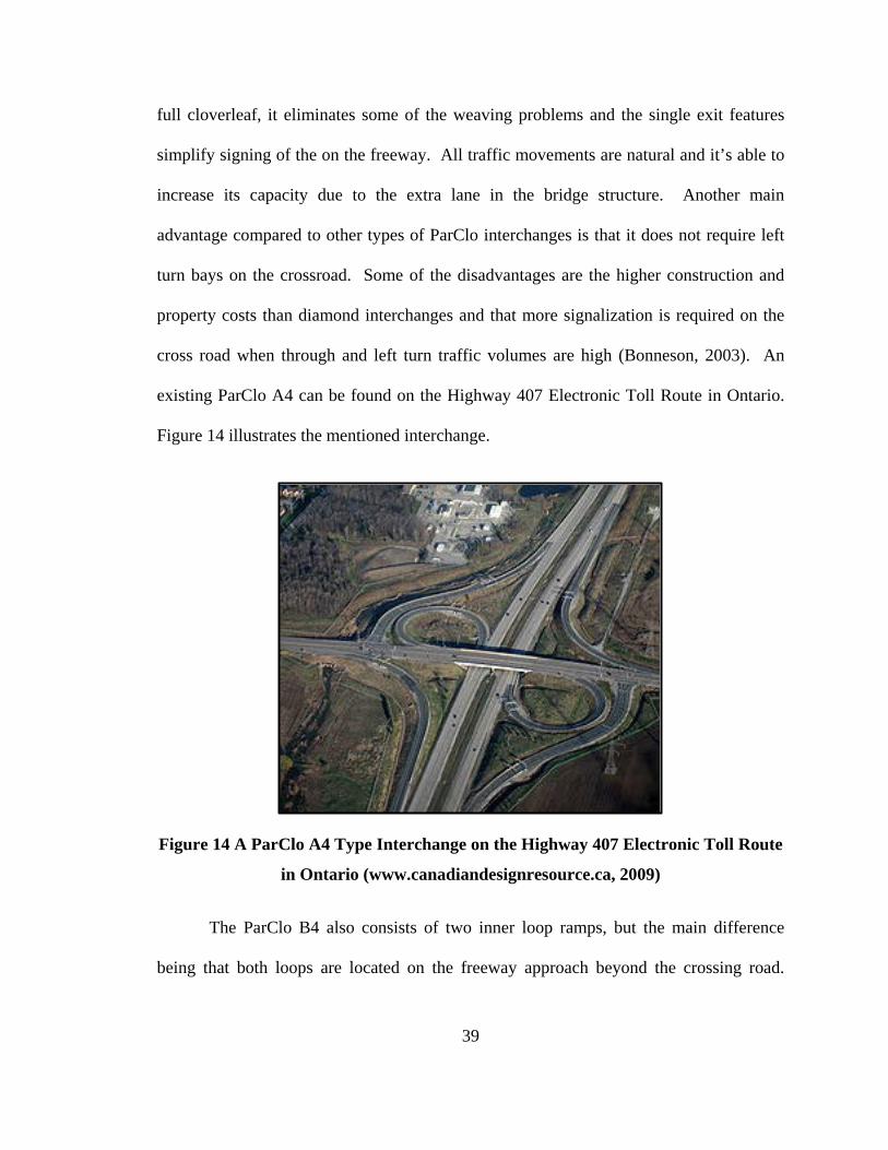
existing ParClo A4 can be found on the Highway 407 Electronic Toll Route in Ontario.
Figure 14 illustrates the mentioned interchange.
Figure 14 A ParClo A4 Type Interchange on the Highway 407 Electronic Toll Route
in Ontario (www.canadiandesignresource.ca, 2009)
The ParClo B4 also consists of two inner loop ramps, but the main difference
being that both loops are located on the freeway approach beyond the crossing road.
Page 53
40
Both of these loop ramp serve as exits from the mainline. In the ParClo B4, the signals
are also controlled by a 2-phase operation, but the movements are very different. Firstly,
the left turn movements are made trough loop ramps and secondly, the left turn
movements from the cross road are made through at-grade intersections. This type of
interchange also increases capacity not just because of the extra lane in the bridge
structure but because one through movement at each intersection does not have to stop.
This has shown to be the major contributor to the decrease of the overall delay of the
interchange (MTO, 1994).
Figure 15 ParClo B4 (MnDOT, 2001)
Some of the main advantages of the ParClo B4 are that movements from the
freeway do not have to pass through a signal, so it significantly reduces the possibility of
Page 54
41
traffic up on the freeway. The single exits on the freeway simplify signing, making it not
conducive to wrong way movements. Some of the other advantages are that weaving is
reduced compared to a full cloverleaf, all the traffic movements are natural and one
through movement at each intersection can receive a continuous green indication
(Bonneson, 2003).
Compared to the ParClo A4, the ParClo B4 has some serious disadvantage.
Traffic exiting from the freeway at high speed is required to decelerate significantly to
negotiate the small radius loop ramp. This feature surprises some drivers and it tends to
have higher accident rates. Also, since one through movement at each intersection does
not have to stop, it makes it more difficult for pedestrians to cross the minor road
(MnDOT, 2001). Another downside compared to a ParClo A4 is that it requires left turn
bays on the crossroad. Compared to diamond interchanges, this type of interchange has
higher construction and property costs (MTO, 1994).
ParClo B4 interchanges can be found in British Columbia, Massachusetts,
Michigan, Nebraska, and Kentucky among other places. An existing ParClo B4, which is
shown in Figure 16, can be found in Woodhaven Wayne in Michigan.
Page 55
42
Figure 16 A ParClo B4 Type Interchange in Woodhaven Wayne, MI
(Google Earth, 2011)
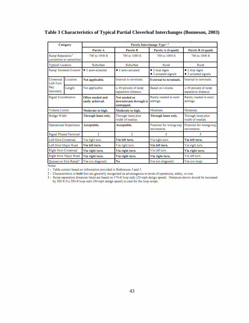
A summary of the characteristics of ParClo Interchanges for the ramp terminal
control, ramp separation, Signal Phasing and volume limits among others can be seen in
Table 3. “ParClo A” and “ParClo B” are understood to have ramps in all 4 quadrants. In
this study, ramp separation is shown to be 700 ft, but according to the Minnesota
Department of Transportation’s Road Design Manual, intersection distance for the
ParClos is between 600 and 900 ft.
Page 56
43
Table 3 Characteristics of Typical Partial Cloverleaf Interchanges (Bonneson, 2003)
Page 57
44
Experimental Design
The operation of an interchange is affected by many factors such traffic volume
conditions present, geometric features and signal plan configuration among others. To
make a fair and realistic comparison, one needs to make sure that the interchanges being
compared have the same characteristics applicable to each type since otherwise one
would be giving advantage to one type of interchange versus the other. One tool that has
effectively been used to compare interchange has been Micro-simulation. The type of
Microsimulation used in this study is AIMSUN 6.0, which is explained in more detail in
the following section. Different Measures of Effectiveness (MOEs), extracted from
Microsimulation, are used to determine how one interchange operates compared to
another. For each model, geometrical characteristics such as the distance between
crossings were property designed to meet standard geometrical design regulations.
Different traffic flows were considered to be tested, where each different flow was further
divided into balanced and unbalanced conditions between the on/off ramp and the
crossroad. To get optimum results for each interchange under the different traffic
patterns, and to compare the interchanges at their best performances, a signal
optimization tool called Synchro was used to optimize the cycle lengths. Each of the
above criterions is described in more detail in the following sections.
Microsimulation Platform
These days the focus of transportation projects has shifted from building more
roads to inventing new unconventional and innovative designs that will help in sustaining
all the traffic growth. One tool to compare operational efficiency of new designs
Page 58
45
compared to conventional ones is by the use of simulation. Simulation modeling provides
researchers and transportation engineers the means to remotely study and analyze traffic
by accurately modeling field conditions. Nowadays simulation is being employed more
often since there are several limitations with the methodology suggested in the Highway
Capacity Manual (Traffic Analysis Tools Primer, 2003).
Simulation tools are effective in evaluating the dynamic evolution of traffic
congestion problems on transportation systems. By dividing the analysis period into time
slices, a simulation model can evaluate the buildup, dissipation, and duration of traffic
congestion (Xiao, 2005). Simulation tools, however, require an excess of input data,
considerable error checking of the data, and manipulation of a large amount of potential
calibration parameter. Simulation models cannot be applied to a specific facility without
the calibration of those parameters to the actual conditions in the field. Calibration can be
a complex and time consuming process (Xiao, 2005). Simulation modeling is being used
increasingly as an off-line tool for testing various controls and for selecting and
evaluating alternative designs before actual implementation. Several traffic simulation
models have been developed for different purposes over the years (Xiao, 2005).
AIMSUN which stands for “Advanced Interactive Microscopic Simulator for
Urban and Non-Urban Networks” was developed by the Department of Statistics and
Operational research, at the Universitat Poletecnica de Catalunya, Barcelona, Spain as a
simulator tool that is able to reproduce real traffic conditions of different traffic networks.
Aimsun has been designed and implemented as a tool for traffic analysis to help traffic
engineers in the design and assessment of traffic systems. The version that was used in
this study was AIMSUN 6.0. Aimsun has two components that allow dynamic
Page 59
46
simulations, the Microscopic Simulator and the Mesoscopic simulator. Both of these
simulators can deal with different traffic networks: urban networks, freeways, highways,
ring roads, arterials and any combination between them (Transport Simulation Systems,
2008).
Throughout the simulation time period, the AIMSUN Microsimulator
continuously models the behavior of every vehicle traveling through the traffic network.
Different vehicle behavior models such car following and lane changing are used in the
Microsimulator. This Microscopic simulator is a combined discrete/continuous
simulator, meaning that there are some elements of the system whose states change
continuously over simulated time. Some other characteristics of AIMSUN are that it
provides detailed modeling of the traffic network, it can distinguishes between different
types of vehicles and drivers, and it enables a wide range of network geometries to be
dealt with, and it can also model incidents, conflicting maneuvers and much more
(Transport Simulation Systems, 2008). These characteristics came in very handy for this
study since DDI consists of a very special geometry.
For traffic generation, the time interval between two consecutive vehicle arrivals,
also known as the headway, is sampled as a random distribution model. When loading a
traffic demand into Aimsun the user may select among different headway models:
exponential, uniform, normal, constant, etc. (Transport Simulation Systems, 2008). For
this study traffic arrivals were assumed as Poisson with the exponential distribution
headways. The outputs provided by AIMSUN Dynamic are a continuous animated
graphical representation of the traffic network performance, both in 2D and 3D, statistical
output data (flow, speed, journey times, delays, stops), and data gathered by the simulated
Page 60
47
detectors (counts, occupancy, speed) (Transport Simulation Systems, 2008). The
animation output is very powerful because it enables the analyst to quickly see and
qualitatively assess the overall performance of each interchange alternative. The reader
can refer to the AIMSUN user’s manual for a more complete description of this
simulation tool. To enable for a direct comparative assessment of the interchange types,
system-wide measures of effectiveness were calculated within AIMSUN.
Measures of Effectiveness
Measures of Effectiveness (MOEs) are the system performance statistics that best
characterize the degree to which a particular alternative operates. To make a fair
comparative assessment of the interchanges in this study and to determine the appropriate
performance criteria, several MOEs were chosen based on several factors. The most
significant factor taken into consideration was delay time, which was the primary
measure of effectiveness used to evaluate the performance of the interchange designs.
Delay is a standard parameter used to measure the performance of an intersection. The
Highway Capacity manual identifies delay, which is used to calculate the level of service,
as the primary measure of effectiveness for signalized intersections (Transportation
Research Board, 2000).
A study by Abbas et. al., (2009) used delay measures as the primary performance
criteria to compare the Single Point Interchange (SPI) to the Diverging Diamond
Interchange (DDI). So from a delay perspective, several performance criteria will be
used to compare the operations of each design. The designs will be tested for several
traffic scenarios, therefore different delay measure such as average delay time, average
Page 61
48
stop time and average number of stops will be accounted for. The number of stops will
clarify the number of times, on average, a driver will have to stop while travelling
through each type of interchange.
A study by Bared et. al., (2005) evaluated and compared the Diverging Diamond
Interchange to a Conventional Diamond Interchange, and the performance measures that
were used for the intersection designs were average delay time per vehicle, average stop
time per vehicle, average number of stops per vehicle, average queue length and
maximum queue length. Another study by Milam et. al. (1999) compared traffic
operations of an existing full cloverleaf interchange with that of a partial cloverleaf
interchange configuration. The key MOEs that were considered for the above study were
total trips served, average travel speed, vehicle miles traveled, vehicle hours of delay and
maximum queue lengths. Therefore maximum queue will also be used as a performance
measure.
The performance statistics that are considered to conduct the operational
comparison of the interchanges from AIMSUN at the system level (i.e. referring to the
entire network) are Delay time, Stop time and Number of stops. AIMSUN defines delay
time as the average time per vehicle, which is the difference between the expected travel
time and the travel time. Stop time is defined as the average time at standstill per vehicle
and number of stops is defined as average number of stops per vehicle. The performance
statistic that is considered at the section level and turning level is maximum queue length
which is defined as the maximum length of the queue in a section, expressed as number
of vehicles per lane. The mean length of a vehicle in AIMSUN is about 13 feet. All of
Page 62
49
these MOEs are calculated as the average of all vehicles (Transport Simulation Systems,
2008).
Based on the criteria presented in this section, average delay, stop time, number of
stops and maximum queue will be the measures of effectiveness selected to evaluate and
compare the operational performance of each interchange design. These MOEs would
effectively demonstrate the actual time wasted for the signals, as well as the
psychological frustrations of the drivers.
Geometrical Features
To accurately code roadway geometry in the simulator, maps were used as
backgrounds. Small background maps were required to distinguish the basic geometric
elements including the start/end points of ramps and weaving sections, number of lanes
and stop lines. The diverging diamond interchange at I-44 and Route 13 in Springfield,
MO was used as reference when drawing the models in AutoCAD and AIMSUN. This
interchange is shown in Figure 10 in the interchange background section.
Figure 17 shows the AutoCAD drawing for the Diverging Diamond Interchange
design that will be used to conduct the comparison. The crossroad in this model has two
lanes in each direction. The through and left turning vehicles cross over to the left side of
the roadway. The left turn movement shares the second lane with the through movement
before the first ramp terminal and then takes the exit ramp before the second ramp
terminal. This eliminates the need for an exclusive left turn bay and a left turn signal
phase, permitting the use of a two phase traffic signal. There are two lanes on the off-
ramps, one for the right turn movement, which is controlled by a yield, and the other for
Page 63
50
the left turn movement which is controlled by a traffic light. The on-ramps consist of the
right turn movement and the left turn movement merging into one single lane. Right turn
movements are controlled by a yield and left turns to access the freeway are done freely.
The distance on the bridge structure (i.e. between the crossings) is approximately 500 ft,
with the total length of the model approximately reaching 1,400 ft in length. These
dimensions are shown in Figure 17.
Figure 17 AutoCAD Drawing for the Diverging Diamond Interchange
Figure 18 shows the AutoCAD drawing for the Partial Cloverleaf type A4
Interchange design. The crossroad in this model consists of two lanes in each direction.
The ParClo A4 consists of four on-ramps and two off-ramps. The on-ramp left turn
movements to access the freeway are conducted via an exclusive loop ramp. This
merging lane adds an extra lane to the bridge structure, which is an advantage compare to
the DDI. The right turn movements for the on-ramp are done freely. Similar to the DDI,
there are two lanes on the off-ramps, one for the right turn movement, which is controlled
by a yield, and the other for the left turn movement which is controlled by a traffic light.
N
Page 64
51
The distance for the bridge structure is approximately 600 ft, with the total length of the
model approximately reaching 1,400 ft.
Figure 18 AutoCAD Drawing for ParClo A4
Figure 19 shows the AutoCAD drawing for the Partial Cloverleaf Interchange
type B4 design. The crossroad in this model consists of two lanes in each direction. The
ParClo B4 consists of two on-ramps and four off-ramps. The on-ramp right turn
movements are conducted by free right turn movements that merge with the left turn
movements from the cross road. The left turn movements from the crossroad are
conducted by an exclusive lane on the bridge structure. There are two ways to access the
crossroad from the freeway. Right turn movements from the off-ramp are conducted
before passing the bridge structure by a single lane that enters the crossroad by yielding
to the through movement. The left turn movements from the freeway to access the
crossroad are conducted via loop ramps. These loop ramps are accessed after going
N
Page 65
52
under the bridge structure, and then merge into the through traffic on the crossroad. This
merging lane and the left turn exclusive lane on the bridge structure add an extra lane to
the bridge structure. This extra lane will also give advantage to this type of interchange
compared to the DDI with a total of 4 through lanes since it will increase capacity. The
distance for the bridge structure is approximately 600 ft, with the total length of the
model approximately reaching 1,400 ft.
In the case of the AutoCAD drawings for ParClo interchanges, the freeway
segment is shown so that the loop connections to the freeway segment can be better
understood. When conducting the micro-simulation model, the freeway segment will not
be considered.
Figure 19 AutoCAD Drawing for ParClo B4
The above models with the described geometries will me compared using the
AIMSUN micro-simulation tool to determine how the DDI compares to the ParClos.
One main characteristics of the ParClo interchange is that it consists of 6 lanes on the
N
Page 66
53
bridge section (2 through and 1 left turn in each direction), and that extra lane compared
to the DDI with 4 through lanes can be very easily converted to a through lane. In terms
of cost, building an extra lane for a DDI would not be more costly than building the
Partial Cloverleaf designs. Therefore a DDI with 6 through lanes will also be modeled to
be compared against the ParClos.
Safety Analysis
A conflict point is the point at which a highway or roadway user crosses, merges
or diverges with another highway or roadway user. Conflict points are commonly used to
explain the accident potential of a roadway. Access management strategies are typically
designed to reduce the number and density of conflict points. Figure 20 is an illustration
of the different conflict points that occur at a DDI interchange. In this type of
interchange, 6 diverging, 6 merging and 2 crossing conflict points take place. Therefore,
there are a total of 14 conflict points.
Figure 20 Diverging Diamond Interchange Conflict Points
Diverging
Merging
Crossing
Page 67
54
Figure 21 is an illustration of the different conflict points that occur at a ParClo
type A4 interchange. In this type of interchange, 6 diverging, 4 merging and 2 crossing
conflict points take place. Therefore, there are a total of 12 conflict points.
Figure 21 ParClo A4 Conflict Points
Figure 22 is an illustration of the different conflict points that occur at a ParClo
type B4 interchange. In this type of interchange, 4 diverging, 6 merging and 2 crossing
conflict points take place. Therefore, there are a total of 12 conflict points.
Diverging
Merging
Crossing
Page 68
55
Figure 22 ParClo B4 Conflict Points
The Diverging Diamond Interchange type has two more conflict points than the
ParClo types, but the conflict points at a DDI are all separated. Three of the conflict
points for a ParClo A4 occur at one of the intersections and for the ParClo B4 two
conflict points occur at an intersection. Therefore, one can make the statement that the
DDI will be less prone to potential accidents since all the conflict points are separated.
Signal Settings and Signal Optimization tool
The next step of analysis was to provide signal timings for each volume range.
Signal timings are critical functions for any type of interchange, therefore signal
optimization software Synchro was used to evaluate signal timings for the interchange
model and only minor adjustments were made by the user.
Synchro, a software developed by Trafficware, is a macroscopic analysis and
optimization tool that implements the methods of the 2000 Highway Capacity Manual.
Synchro allows for quick generation of optimum timing plans, where it optimizes cycle
Diverging
Merging
Crossing
Page 69
56
lengths, split times, offsets and phase sequences to minimize driver stops and delay
(Husch et. al., 2006). Before any optimization can begin, it is very important to
understand the functions that this type of software might use. Synchro contains a number
of optimization functions which are shown in Figure 23.
Figure 23 Synchro’s Optimization Functions (Husch et. al., 2006)
The first step in optimizing an intersection is to set up timing plans, where volume
data, lane data, Phase numbers for each movement along with phase parameters will be
some of the required factors. This step also covers optimization of cycle lengths and
splits, and the determination of capacity and coding errors. The second step requires the
division of the network into subsystems so that each zone can be optimized as a separate
structure in the cycle length optimization. Since in this study only one interchange will
be optimized at a time, this step was skipped. The third step is to optimize the cycle
length for the system. Synchro sets up a timing plan for each cycle length, and then
Page 70
57
selects the cycle length that will best perform based on different Measures of
Effectiveness (MOE). The last step optimizes offsets as well as the phase order if the
option of “Allow Lead/Lag Optimize” is selected, which was the case for this study. This
Lead/Lag optimization will check al combinations of leading and lagging phasing to
improve traffic flow (Husch et. al., 2006).
Signal optimization software Synchro has the ability to model multiple
intersections with one controller also known as group control. This feature of Synchro,
called “Cluster Editor”, allows for the analysis of complex traffic situation such as a
diamond freeway interchange or two closely spaced intersections, which are the case for
the DDI and ParClo interchanges (Husch et. al., 2006). Having one controller will also
help in coordinating both intersections, so that travel for drivers is smooth.
The amber time interval used, which is the amount of time for the yellow interval,
was 3 seconds and all-red interval, which is the amount of time for the all read interval
that follows the yellow interval, was set at 2 seconds after each phase ends. The 2
seconds interval should be of sufficient duration to permit the intersection to clear before
cross traffic is released. Also, free right turn movements were allowed and priority rule
was coded in the model. After all the characteristics of each interchanged were modeled
in Synchro, each design was run for 3600 seconds, to determine the optimum cycle length
for each of the scenarios for the different volume ranges. Each design is described in
more detail in the following paragraphs.
Signal phasing diagram for the DDI is shown in Figure 24. Whether or not all
movements within the DDI are signal controlled, each signal should be timed as a two-
phase signal. This two-phase operation permits for a shorter cycle lengths and decreased
Page 71
58
lost time per phase. Careful attention should be given to the traffic distribution at the
interchange to determine movements that should receive priority (Siromaskul, 2010).
Therefore, all the scenarios were simulated in Synchro to determine the optimum cycle
length pertaining to each traffic distribution.
Figure 24 Movements and Phase Numbering Scheme for the DDI
The optimum cycle lengths obtained from Synchro are shown in Table 4. All of
the optimum cycle lengths are based on traffic data that corresponds to each scenario. An
important observation to note is that when one lane was added to the DDI, the optimum
cycle length dropped from 100-130 seconds to 60-80 seconds, which is a big difference
and will result in lower delays for potential users.
Page 72
59
Table 4 a) Optimum Cycle Lengths for DDI with 2 Thru Lane b) Optimum Cycle
Lengths for DDI with 3 thru lane
a) b)
Traffic Volume
Scenario
Optimum Cycle
Length (sec)
Traffic Volume
Scenario
Optimum Cycle
Length (sec)
High 3 100-130 sec High 3 60-80 sec
High 2 90-110 sec High 2 60-80 sec
High 1 75-100 sec High 1 55-70 sec
Medium 50-55 sec Medium 50 sec
Low 50 sec Low 50 sec
Figure 25 is an illustration of one of the signal timing plans for one of the
scenarios for the DDI. The first phase of the interchange is controlled by phases Ø1, Ø3
and Ø6 and the second phase is controlled by phases Ø2, Ø5 and Ø4. This phase order
was determine by Synchro to be the optimum order. The signal timing plan figure shows
the optimum signal phasing scheme as well as the duration for each phase.
Figure 25 Optimal Signal Timing Plan for DDI 4 High 3.1 Volume Scenario
Page 73
60
For this study, Partial Cloverleaf interchanges with closely spaced intersections
were studied. In a ParClo A4 interchange, the signals are controlled by a 2 phase
operation. The signal phases for the ParClo A4 are illustrated in Figure 26.
Figure 26 Movements and Phase Numbering Scheme for the ParClo A4
Figure 27 illustrates one of the optimal signal timing plans obtained from Synchro
for the ParClo A4 Interchange. Table 5 contains all the optimal cycle lengths that were
measured for all the scenarios and traffic volumes. The first phase of the interchange is
controlled by phases Ø1, Ø2, Ø4 and Ø5 and the second phase is controlled by phases Ø3
and Ø6. This phase order was determine by Synchro to be the optimum order. Figure 27
illustrates the signal phase scheme for the High 3.1 traffic scenario for the ParClo A4
along with the duration of each phase.
Page 74
61
Figure 27 ParClo A4 Optimal Signal Timing Plan for High 3.1 Volume Scenario
The ParClo B4 is also controlled by a 2 phase operation, but the signal setting is
much different. An illustration of the signal settings can be observed in Figure 28.
Figure 28 Movements and Phase Numbering Scheme for the ParClo B4
Figure 29 illustrates one of the optimal signal timing plans obtained from Synchro
for the ParClo B4 Interchange. The first phase of the interchange is controlled by phases
Ø2, Ø3, Ø4 and Ø6 and the second phase is controlled by phases Ø1, Ø3, Ø5 and Ø6.
This phase order was determine by Synchro to be the optimum order. For this type of
interchange, phases Ø3 and Ø6 will have green for the entire cycle length since there are
Page 75
62
no conflicts with other movement. This characteristic makes it very hard to have
pedestrian crossings.
Figure 29 ParClo B4 Optimal Signal Timing Plan for High 3.1 Volume Scenario
Table 5 illustrates the optimum cycle lengths for the ParClo A4 and ParClo B4
interchanges. In terms of the cycle length, compared to the ParClo B4, the ParClo A4
required a much longer cycle length to provide optimal results. The main reason for this
is that in a ParClo B4, one through movement at each intersection does not have to stop.
The optimum cycle lengths for low and medium volumes were very similar for both of
these interchanges, but for the high volume scenarios, the optimum cycle length changed
significantly.
Page 76
63
Table 5 a) Optimum Cycle Lengths for ParClo A4 b) Optimum Cycle Lengths for
ParClo B4
a) b)
Traffic Volume
Scenario
Optimum Cycle
Length (sec)
Traffic Volume
Scenario
Optimum Volume
Scenarios
High 3 90-150 sec High 3 55-60 sec
High 2 90-130 sec High 2 50-60 sec
High 1 80-110 sec High 1 45-55 sec
Medium 40-55 sec Medium 40 sec
Low 40 sec Low 40 sec
Traffic Volume Scenarios
Traffic volumes and patterns in an interchange can change very drastically in a
short period of time, and this alters the operational performance of the interchange. In
order to make a better comparison between the interchanges in this study, a variety of
volume scenarios on the same interchange network were simulated to keep the geometric
conditions constant. The variety of volume scenarios were considered to first achieve a
broad-based comparison of the different interchange designs under similar conditions and
second to test the impact of different magnitudes of traffic volumes. Garber et. al. in an
earlier study recommended that the spectrum of volume scenarios should be extended
from balanced to unbalanced flow conditions. This way the performance of the
interchanges could be examined under field like circumstances. Unbalanced traffic
Page 77
64
volumes are common at morning and afternoon peak periods, especially for commuter
traffic in suburban areas. Therefore this type of scenarios must be tested to fully
understand the effects the interchanges being studied might have if this type of conditions
were to occur (Garber, 1999).
The traffic volumes were expressed in number of vehicles per hour, where traffic
was composed of only two vehicle types, cars and trucks, and corresponding percentage
of 98% and 2% are assigned to them respectively. For this study, 5 different ranges of
volume scenarios were considered. The specific volume scenarios used are:
1. High 3 volume: 6,100 veh/hr
2. High 2 volume: 5,600 veh/hr
3. High 1 volume: 5,100 veh/hr
4. Medium volume: 3,200 veh/hr
5. Low volume: 1,700 veh/hr
Three high volume scenarios were considered to study how each of the
interchanges would perform at higher volumes were capacity might be soon to be
reached.
Table 6 shows how each of the traffic volumes ranges is broken down for the
different movements.
Page 78
65
Table 6 Traffic Movements (Bared et. al., 2005)
Traffic Scenario Eastbound (Veh/hr) Westbound (veh/hr)
Southbound off-ramp (veh/hr)
Northbound off-ramp (veh/hr)
Total Flow
(veh/hr) L T R L T R L R L R
High 3 450 850 550 450 850 550 750 450 750 450 6100 High 2 400 800 500 400 800 500 700 400 700 400 5600 High 1 350 750 450 350 750 450 650 350 650 350 5100
Medium 200 500 300 200 500 300 400 200 400 200 3200 Low 100 300 150 100 300 150 200 100 200 100 1700
The above mentioned volumes provide some insight into the relative operations of
the different types of interchanges, but as mentioned before, Garber et. al. in an earlier
study recommended that the spectrum of volume scenarios should be extended from
balanced to unbalanced conditions. Therefore, the volume scenarios were further divided
into 10 different scenarios to test the impact of different varieties of traffic volumes and
distributions and to gain a better picture on the operational performance of the
interchange.
Table 7 illustrates the pattern as well as the trend of change of the scenarios. In
the table, “Balanced” means that the opposing movements (e.g. northbound and
southbound through) in each phase have the same traffic volume. In the other hand,
“unbalanced” mean that one direction has a higher traffic volume than the other (Abbas,
2009).
Page 79
66
Table 7 Traffic Patterns for Each Volume Range (Abbas, 2009)
Scenarios Crossroad Freeway
Through Movements Left Turns Left Turn off ramps
1 Balanced Balanced Balanced
2 Balanced Balanced Unbalanced
3 Balanced Unbalanced Balanced
4 Balanced Unbalanced Unbalanced
5 Unbalanced Balanced Balanced
6.1* Unbalanced Balanced Unbalanced
6.2^ Unbalanced Balanced Unbalanced
7 Unbalanced Unbalanced Balanced
8.1* Unbalanced Unbalanced Unbalanced
8.2^ Unbalanced Unbalanced Unbalanced
* Heavier through volume opposes the heavier left-turn volume
^ Heavier through volume opposes the lighter left-turn volume
Moving down on Table 7, the directional distribution of the traffic goes from a
balanced to an all unbalanced condition. For example, all movements for scenario 1 will
have the same traffic volume for opposing movements, whereas for scenario 8, all
movements will have different opposing traffic volumes. In needs to be mentioned that
for scenarios 6.1, 6.2, 8.1 and 8.2, the distribution of the balanced and unbalanced
conditions is the same. The main difference is that for scenarios 6.1 and 8.1, the heavier
Page 80
67
through volume opposes the heavier left turn traffic volume and for scenarios 6.2 and 8.2,
the heavier through volume opposes the lighter left turn volume.
Table 8 shows the distributions for the High 3 volume scenario. For the
distribution of the rest of the traffic flows, refer to the Tables in the Appendix. It must be
mentioned that for all the scenarios, right turn movements for the crossroad were fixed,
and for the “unbalanced” conditions, the larger movement was twice the smaller
movement.
Table 8 Distribution of Traffic Volumes for the “High 3” Volume Scenario
Traffic Scenarios
Eastbound Bound Westbound Bound Southbound off-ramp
Northbound off-ramp Total
volume Right Thru Left Right Thru Left Right Left Right Left 1 550 850 450 550 850 450 450 750 450 750 6100 2 550 850 450 550 850 450 600 1000 300 500 6100 3 550 850 300 550 850 600 450 750 450 750 6100 4 550 850 300 550 850 600 600 1000 300 500 6100 5 550 567 450 550 1133 450 450 750 450 750 6100
6.1 550 567 450 550 1133 450 600 1000 300 500 6100 6.2 550 567 450 550 1133 450 300 500 600 1000 6100 7 550 567 300 550 1133 600 450 750 450 750 6100
8.1 550 567 300 550 1133 600 600 1000 300 500 6100 8.2 550 567 300 550 1133 600 300 500 600 1000 6100
Model inputs and development
So far we have seen the geometry of the interchanges that will be modeled, the
different scenarios that will be simulated as well as the different optimum cycle lengths
that were extracted from the signal optimization software Synchro. On this section we
will see how the models were built in the micro-simulation. Once all the assumptions
were made about the geometry of the interchanges and the cycle lengths were optimized,
all the data was inputted into the AIMSUN software. To develop the models, AutoCAD
Page 81
68
drawings were used as backgrounds. Figure 30 shows the model for the DDI with four
through lanes modeled in AIMSUN. In this case the crossroad is shown in the
north/south direction and the freeway would supposedly be traveling east/west direction.
The geometry of the DDI was described in the geometrical features section.
Figure 30 AIMSUN Model for DDI-4
Figure 31 is an illustration of ParClo types A4 and B4. Again in this image the
crossroad is shown in the north/south direction and the freeway would supposedly be
traveling east/west direction. For the detail explanation of the geometry, refer back to the
geometrical feature section.
Page 82
69
Figure 31 AIMSUN Models for a) ParClo A4 and b) ParClo B4
Once all models were created they were properly examined to make sure no
mistakes were made about the geometrical features and to make sure that all the data was
entered correctly. The same traffic volumes as well as the same lane configuration were
applied to all of the redesigned interchanges. Signal timings used for the designs were
the ones obtained from Synchro and were then modified by the user though several trials
to improve the performance. Extensive computer simulations of the interchange types
were performed in order to determine traffic characteristics that affected operations at the
interchanges. The variation of traffic demand volumes generated a total of 50 scenarios
for each interchange design. Simulation time for each run was 7,200 seconds and the
warm up period was set to 900 seconds for each model. Simulation runs were performed
on the same computer to ensure consistency since otherwise a simulation could be
affected by the type of computer used. The memory and the processor of the computer
that was used were Intel® Core™ i5 CPU 3.20 GHZ, 4.00 GB of RAM.
Page 83
70
Because of traffic variability, a statistically calculated number of runs were
necessary to achieve a level of confidence in the results. Results of a study conducted by
FHWA, who tried to examine the validity of computer models for a case study using
CORSIM, showed that between 5 and 10 different runs showed recognizable
improvements in terms of achieving the mean value and that at least 10 simulation runs
were needed to stabilize the results due to traffic variability (Wiegand et. al., 2011).
Therefore, 10 replications were performed for each simulation to ensure that there were
no significant discrepancies in the results.
The number of seeds used also affects the results of a simulation run. For
instance, if ten replications are performed with the same number of seeds, the ten
replications will yield the same results. Therefore, different seed numbers were used for
each of the ten simulation runs. Different random seed values are assigned to each
replication in AIMSUN by default. In case an inconsistency was observed in the
preliminary results between the different replications, the entire animation simulation was
observed in order to select the problem and fix it. An average of the replications was
then computed. Once everything was observed to be properly working, the necessary
measures of effectiveness were extracted from the micro-simulation platforms for
statistical analysis and comparison between the intersection designs. The results of these
simulations helped to gain insight into the relative performance of the interchange types
therefore showing the differences in their operational capacities.
Page 84
71
ANALYSIS AND RESULTS
As mentioned before, the key simulation MOEs that were considered in the
analysis included Delay time, Number of Stops, Stop time and Maximum queue length.
The same input traffic volumes were applied to all designs. In this way, the performance
measures from the designs been studied in this research are comparable. On the
subsequent figures and tables, a comparison is done for all three types of interchanges
(four if we consider the DDI with 4 thru lane and the DDI with 6 through lanes) which
are shown in a graphical and tabular format. Results are divided into the five different
traffic flows (high3, high 2, high 1, medium and low) and different graphs and tables are
created to represent the different MOEs.
Table 9 shows the results for the balanced flow conditions for all the interchanges.
In this research, all balanced conditions occurred in Scenario 1, where all the movements
have balanced conditions. The performance of the interchanges for lower and medium
volumes is very similar for all designs, but results still indicate that the ParClo B4
outperforms the other interchanges. Both ParClo type interchanges show much better
results compared to the DDI in terms of Delay time (where there is a decrease in delay of
2.77 to 5.24 sec/veh), Stop time (which is close to 54% lower) and Number of Stops
Page 85
72
(where again the distinction is significant with close to 42% lower number of stops). In
terms of queue at low volumes, the ParClo A4 experienced a smaller queue consisting of
4 vehicles, 16-33% lower than the other interchanges. For Medium volumes, the ParClo
B4 again outperformed the other interchange types. In terms of delay, the ParClo B4 had
2.66 seconds lower delay compared to the ParClo A4, and 5.31 seconds lower compared
to the DDIs. In terms of queue in Medium volumes, the DDIs and the ParClo B4
experienced an increase of 1 to 1.5 vehicles from low to medium volume, where the
ParClo A4 experienced an increase of 4.5 vehicles, which is an increase of 53%.
Having a lower Delay and Number of stops for the ParClo B4 was expected since
one through movement at each intersection does not have to stop, therefore decreasing
these MOEs being considered to evaluate the interchanges. As was mentioned before,
the main reason to have a 4 lane DDI and a 6 lane DDI in this study was that if the DDI
with 4 thru lanes turned out to perform worse than the ParClo interchanges with the same
amount of thru lanes, then one could make the assumption that constructing a DDI with
one extra lane per direction compared to the ParClos with 4 lanes would not be more
costly. This is because of the acceleration/deceleration lanes in the bridge structure that
act as an extra lane.
As illustrated in Table 9 below, the DDI with 4 through lanes did not perform as
well as the other interchanges. In terms of Delay time, the DDI-4 had the largest value
followed by the ParClo A4, the DDI-6 and ParClo B4. Compared to the ParClo B4, the
DDI-4 and ParClo A4 had at least double the delay if not more for all the High flows.
But comparing the DDI with 6 through lanes with the ParClo B4, it can be observed that
as the flows increased, the difference between their delay times decreased, to the point
Page 86
73
that by High-3 flow scenario, the delay times almost came to be equal. The ParClo B4
went from a Delay time of 8.45 sec/veh to a delay of 13.9 sec/veh (an increase of 64.5%),
where the DDI-6 only changed from a delay of 12.9 sec/veh to a delay of 14.1 sec/veh
(an increase of 9.3%). An assumption could be made that if higher volumes would have
been studied, then the DDI-6 would have outperformed the ParClo B-4.
Regarding stop time, the DDI-6 had the smaller value for the High-3 traffic flow
followed by the ParClo B4, ParClo A4 and DDI-4. It can be noted that the stop time for
the vehicles in the DDI-6 interchange was not affected as much when the traffic flow was
increased, since from High-1 to High-3 flows the stop time only increased by 6%,
compared to an increase of 95% for the ParClo B4.
In Table 9 we can observe that for all the High traffic flows, the ParClo B4
outperformed the rest of the Interchanges except in Maximum queue. For High-3 volume
flows, the ParClo B4 had a 158% higher queue than the DDI-4, 207% higher queue than
the DDI-6 and a 48% higher queue than the ParClo A4. Increasing the amount of cars
had a greater impact in term of queue for the ParClo B4, since after High-1 traffic flow
scenario, the maximum queue grew more substantially compared to the other
interchanges. The reason why this happened was that at high traffic volumes, the cars
coming off the freeway had a hard time accessing the crossroad. The through movements
in the crossroad have green throughout the whole cycle length, which means that they
will never stop, consequently they do not allow enough space for the cars coming off the
freeway to merge onto the crossroad.
The lowest queues for the High traffic flow scenarios corresponded to the DDI
with 6 through lanes, which was expected, since having an extra lane per direction would
Page 87
74
help in decreasing the queue. An interesting observation was that the maximum queues
for the DDI-6 were not that different from the DDI-4, which is due to the special
geometry of this interchange. If only the interchanges with 4 through lanes are
considered, then in terms of queue the DDI-4 outperformed the ParClos for the High-3
scenarios. The DDI-4 had a 42% fewer queue compared to the ParClo A4 and 61%
reduction compared to the ParClo B4.
To conclude with the balanced condition results, it needs to be mentioned that for
maximum queue, from the low traffic flow to the High 3 traffic flow, the ParClo B4
experienced the highest change. It went from having a queue of 5 vehicles at low flows
to having a maximum queue of 40 vehicles, which is an increase of 700% compared to an
increase of 158% for the DDI-4, 116% for the DDI-6 and 575% for the ParClo A4
design.
Page 88
Table 9 Results for All Balanced Conditions
Traffic Flow
Scenario
Input Flow
(Veh/hr)
Delay Time (sec/veh) Stop Time (sec/veh) No. of Stops Max. Queue (veh)
DD
I-4
DD
I-6
ParClo A
4
ParClo B
4
DD
I-4
DD
I-6
ParClo A
4
ParClo B
4
DD
I-4
DD
I-6
ParClo A
4
ParClo B
4
DD
I-4
DD
I-6
ParClo A
4
ParClo B
4
High 3 6,100 32.6 14.1 30.1 13.9 25.5 8.81 20.9 9.5 0.837 0.595 0.939 0.496 15.5 13 27 40
High 2 5,600 21.9 13.4 20.06 10.1 15.9 8.52 12.9 6.24 0.696 0.554 0.606 0.399 12 12 23 27
High 1 5,100 18.9 12.9 16.6 8.45 13.4 8.27 10.3 4.87 0.635 0.532 0.518 0.365 11.5 10 18 15
Medium 3,200 11.4 11.3 8.75 6.09 7.18 7.18 4.12 3.29 0.515 0.501 0.358 0.285 7.5 7 8.5 6
Low 1,700 10.2 9.89 7.43 4.96 6.63 6.48 3.47 2.73 0.475 0.465 0.317 0.24 6 6 4 5
75
Page 89
76
Table 10 shows the results for the unbalanced flow conditions for all the
interchanges. Unbalanced conditions mean that each opposing direction will have double
the amount of vehicles than the other opposing direction. In this research, all movements
had unbalanced conditions for Scenarios 8.1 and 8.2. Table 10 shows the results for
Scenario 8.2. The performance of the interchanges for lower and medium volumes is
very similar for all designs, but results still indicate that the ParClos perform better than
the DDIs for these types of conditions. Overall, the ParClo B4 still had the lowest delay
time, stop time, number of stops and maximum queue for low and medium volumes.
A considerable observation was that the DDI-4 performed better than the ParClo
A4 at high volumes for the unbalanced conditions, which wasn’t the case in the balanced
scenarios. At High-3 traffic flows, the DDI-4 had a delay of 33.7 sec/veh compared to
43.2 sec/veh for the ParClo A4. The impact on the delay done from changing from
balanced conditions to unbalanced traffic conditions at High-3 volume was much more
substantial for the ParClos than it was for the DDIs. The DDI-4 and DDI-6 had a percent
increase of 3.37% and 12.8% respectively, compared to the percent increase of 43.5% for
the ParClo and 30.9% for the ParClo B4.
With respect to stop time at very high volumes, the DDI-6 had the lowest value
followed by the ParClo B4 for the unbalanced conditions, which was the same case when
balanced conditions were present. But for the DDI-4 and ParClo A4, the ParClo A4 had
a lower stop time at balanced conditions compared to the DDI-4, but for the unbalanced
conditions, the DDI-4 was observed to have a smaller stop time value.
Regarding number of stops, the DDI-6 had the lowest value, which was followed
by the ParClo B4, DDI-4 and ParClo A4. For number of stops, one main observation was
Page 90
77
that the ParClo A4 had almost double the stops during the unbalanced conditions
compared to the balanced condition, whereas the DDI’s number of stops where almost
constant. In terms of queue, the DDI-6 had the lowest values for High traffic volumes.
But if we again compare the interchanges with 4 through lanes, then again the DDI-4
outperformed both ParClos.
Page 91
Table 10 Results for All Un-balanced Conditions
Traffic Flow
Scenario
Input Flow
(Veh/hr)
Delay Time (sec/mile) Stop Time (#/veh/mi) No. of Stops Max. Queue (ft)
DD
I-4
DD
I-6
ParClo A
4
ParClo B
4
DD
I-4
DD
I-6
ParClo A
4
ParClo B
4
DD
I-4
DD
I-6
ParClo A
4
ParClo B
4
DD
I-4
DD
I-6
ParClo A
4
ParClo B
4
High 3 6,100 33.7 15.9 43.2 18.2 26.5 10.6 31.9 13.3 0.834 0.58 1.71 0.61 18.5 15 27 49
High 2 5,600 31.4 14.1 37.5 10.7 24.5 9.15 27.1 6.62 0.793 0.561 1.27 0.42 15 14.5 27 25
High 1 5,100 23.1 13.4 32.2 8.71 17.2 8.51 22.6 5.13 0.679 0.556 1.072 0.35 15 14 26 19
Medium 3,200 12.5 11.1 10.1 6.25 8.07 6.96 5.17 3.41 0.533 0.486 0.36 0.29 10 7 12.5 6.66
Low 1,700 9.70 9.65 7.99 5.01 6.20 6.30 3.76 2.77 0.456 0.448 0.33 0.24 6 6 5 4.33
78
Page 92
79
Figure 32 and Figure 33 are illustrations in graphical format of the delay time for
all the traffic flows for each interchange. In each graph, the x-axis represent the different
scenarios (from balanced to unbalanced conditions) discussed on the traffic volume
scenario section, and on the y-axis we have the delay time in seconds per vehicle. In
each table, the light blue color represents the Delay Time for the DDI with 4 through
lanes, the darker blue represents the Delay Time for the DDI with 6 thru lanes, the red
color represents the Delay Time for the ParClo A4 and lastly the green color represents
the Delay Time for the ParClo B4. Graph Figure 33 a) represent the delay time of the
interchanges for the High-3 traffic flow, Figure 33 b) represents the delay time for the
High-2 traffic flow, Figure 33 c) represents the delay time for High-1 traffic flow
scenarios, Figure 32 a) represents the delay time for Medium traffic flow volumes and
Figure 32 b) represents the delay time for Low traffic flow volume.
It was obvious from the graphs that the ParClo A4 and DDI-4 did not perform as
well as the other two interchanges. It was no surprise that the DDI-6 had better results
than the DDI-4 since one extra lane per direction added more capacity, and it was also
not a surprise that in terms of Delay time, Stop time and Number of stops that the ParClo
B4 outperformed the ParClo A4 since as has been mentioned earlier one through
movement on the crossroad for the ParClo B4 does not stop. Therefore, the analysis was
mostly divided into comparing the DDI-4 with the ParClo A4 and the DDI-6 with the
ParClo B4. For Low and Medium volume scenarios, it can be noted that the lowest delay
occurred for the ParClo B4 followed by the ParClo A4. When the scenarios moved from
all balanced to all unbalanced scenarios (i.e. from Scenario 1 to Scenario 8.2), there were
no apparent changes in the graphs.
Page 93
80
a)
b)
0
2
4
6
8
10
12
14
1 2 3 4 5 6.1 6.2 7 8.1 8.2
Dela
y Ti
me
(sec
/veh
)
Scenarios
Low Volume Scenario
DDI-4
DDI-6
Parclo A4
Parclo B4
0
2
4
6
8
10
12
14
1 2 3 4 5 6.1 6.2 7 8.1 8.2
Dela
y Ti
me
(sec
/veh
)
Scenarios
Medium Volume Scenario
DDI-4
DDI-6
Parclo A4
Parclo B4
Figure 32 Results for Delay Time for Low and Medium Scenarios
On the other hand, for High volumes the story is a little different. Firstly, the
ParClo B4 outperforms the rest of the interchanges at all volumes, but as the volumes
became larger, we see that the difference between the DDI-6 and the ParClo B4 starts
getting closer, to the point that at High-3 volume scenario, the average delay for the
ParClo B4 is 14.7 sec/veh for all 10 scenarios and the average delay for the DDI-6 is
15.84 sec/veh. Between the High-1 to High-3 scenarios, the average delay for the DDI-6
Page 94
81
changed from a delay of 13.7 sec/veh to a delay of 15.8 sec/veh, a 15% increase,
compared to the ParClo B4 which went from a delay of 8.62 sec/veh to a delay of 14.7
sec/veh, an increase of 70%. This tells us that for the High scenarios simulated in this
study, the ParClo B4 outperformed the DDI-6, but if higher traffic flows (e.g. 6,600
veh/hr) would have been studied, with almost all certainty the DDI-6 would have
outperformed the ParClo B4.
DDI-6 and the ParClo B4 performed comparable at High-3 scenarios, and we
have stated before that the average delay for all 10 scenarios was lower for the ParClo
B4. But the graph denotes that there are two instances in particular were the DDI-6
outperforms the ParClo B4, which are scenarios 6.2 and 8.2. This indicates that the DDI-
6 would perform better when the heavier through movement on the crossroad opposes the
lighter left turn movement from the ramp.
Now if we analyze the results for the ParClo A4 and the DDI-4 for all High
scenarios we see that for the more balanced scenarios (Scenarios 1 through 4) the ParClo
A4 had a smaller delay time compared to the DDI-4. This suggests that if balanced
scenarios would occur in the field in a real scenario, then the ParClo A4 would be the
more suitable choice. On the other hand, we see that after scenario 4 the DDI-4’s
performance was better than the ParClo A4. So if the conditions in the field behave more
unbalanced, which is the case during peak hour traffic, then the DDI-4 would be a more
appropriate design to implement. The main reason for this occurrence was that a higher
mean queue value was observed for the ParClo A4 than the DDI. Since the vehicles
trying to make a left turn from the off-ramp had to cross the through traffic, then this
increased the delay time since there were cars back up for the major part of the
Page 95
82
simulation. Also the special geometry of the DDI allowed for a lower cycle length,
therefore decreasing the overall delay time. Another observation about the DDI-4 at
High-3 traffic flow was that it performed best for scenario 5, which was when all
movements were balanced except the through movement on the cross road. The ParClo
A4 showed best results for the first four scenarios, where all scenarios had one thing in
common, through movements were balanced.
Page 96
83
0
5
10
15
20
25
30
35
40
1 2 3 4 5 6.1 6.2 7 8.1 8.2
Dela
y Ti
me
(sec
/veh
)
Scenarios
High 1 Volume Scenario
DDI-4
DDI-6
Parclo A4
Parclo B4
0
10
20
30
40
50
1 2 3 4 5 6.1 6.2 7 8.1 8.2
Dela
y Ti
me
(sec
/veh
)
Scenarios
High 2 Volume Scenario
DDI-4
DDI-6
Parclo A4
Parclo B4
0
10
20
30
40
50
60
1 2 3 4 5 6.1 6.2 7 8.1 8.2
Dela
y Ti
me
(Sec
/veh
)
Scenarios
High 3 Volume Scenario
DDI-4
DDI-6
Parclo A4
Parclo B4
a)
b)
c)
Figure 33 Results for Delay Time for High Scenarios
Page 97
84
For Figure 34 and Figure 35, the same colors and characteristics as the graphs
before (e.i. Figure 32 and Figure 33) are used to represent each interchange. The main
difference is that now the y-axis represents the stop time in seconds per vehicles. For low
and medium traffic flows, the ParClos were superior to the DDIs. The values for all
designs stayed fairly constant throughout the 10 different scenarios.
Figure 34 Results for Stop Time for Low and Medium Scenarios
Page 98
85
At High volumes, the ParClo B4 was more superior in terms of stop time to the
rest of the interchanges. But as the traffic flow increased from High-1 to High-3, the
difference from the ParClo B4 to the DDI-6 diminished. The average stop time for all 10
scenarios for the DDI-6 and ParClo B4 at the High-3 traffic flow was 10.45 sec/veh and
10.1 sec/veh respectively, which is very close. Again if we look at the increase of the stop
time value from the High-1 scenario to the High-3 scenario, we can make an assumption
that the DDI-6 will be better at higher volumes which have not been simulated in this
study. For scenarios 1 through 4 (e.i. a more balanced condition), the ParClo B4 had a
lower stop time than the DDI-6, but for a more unbalanced conditions except for
scenarios 6.1 and 8.1, the DDI-6 had a lower delay time. Therefore it would be fare to
say that the DDI-6 would perform better during peak hours at volume higher than 6,100
vehicles per hour (e.i. higher than High-3 traffic flow).
Analyzing the results of stop time for the ParClo A4 and the DDI-4 showed very
similar results as before when the delay time was analyzed for these two interchange
designs. The ParClo A4 was superior for the more balanced conditions, where it showed
its best results. The DDI-4 outperformed the ParClo when more unbalanced conditions
were present (e.i. scenarios 5 through 8.2) and its best results occurred at scenario 5
which was the same case when examining delay time.
Page 99
86
a)
b)
c)
0
5
10
15
20
25
30
35
1 2 3 4 5 6.1 6.2 7 8.1 8.2
Stop
Tim
e (s
ec/v
eh)
Scenarios
High 1 Volume Scenario
DDI-4
DDI-6
Parclo A4
Parclo B4
0
5
10
15
20
25
30
35
40
1 2 3 4 5 6.1 6.2 7 8.1 8.2
Stop
Tim
e (s
ec/v
eh)
Scenarios
High 2 Volume Scenario
DDI-4
DDI-6
Parclo A4
Parclo B4
05
1015202530354045
1 2 3 4 5 6.1 6.2 7 8.1 8.2
Stop
Tim
e (s
ec/v
eh)
Scenarios
High 3 Volume Scenario
DDI-4
DDI-6
Parclo A4
Parclo B4
Figure 35 Results for Stop Time for High Scenarios
Page 100
87
For Figure 36 and Figure 37, the same characteristics for the previous graphs are
used to represent each interchange. The only difference is that in this graphs, the y-axis
is represented by number of stops make by each vehicle. Figure 36 a) and Figure 36 b)
represent medium and low volumes respectively, and it can be noted that the ParClos had
fewer stops than the DDIs.
a)
b)
0
0.1
0.2
0.3
0.4
0.5
0.6
0.7
1 2 3 4 5 6.1 6.2 7 8.1 8.2
Num
ber o
f Sto
ps
Scenarios
Medium Volume Scenario
DDI-4
DDI-6
Parclo A4
Parclo B4
0
0.1
0.2
0.3
0.4
0.5
0.6
0.7
1 2 3 4 5 6.1 6.2 7 8.1 8.2
Num
ber o
f Sto
ps
Scenarios
Low Volume Scenario
DDI-4
DDI-6
Parclo A4
Parclo B4
Figure 36 Results for Number of Stops for Low and Medium Scenarios
Page 101
88
Now moving to the High traffic flows on Figure 37, it can be observed that again
the ParClo B4 performed much better in terms of number of stops compared to the rest of
the interchanges. It can also be noted that as the traffic flows move from a High-1 flow
to a High-3 flow, the number of stops between the ParClo B4 and DDI-6 got closer.
Therefore another assumption can be made that for higher scenarios than represented in
this study, the DDI-6 would have a smaller value for the number of stops.
One main observation is that the number of stops for the ParClo B4, DDI-4 and
DDI-6 remain constant for almost all scenarios except for the High-3 traffic flow. So
changing the conditions in the roadway from balanced to unbalanced conditions did not
have a big effect in these three interchanges. In the other hand, the number of stops made
by vehicles had a great effect when traffic conditions changed for the ParClo A4. We see
that for balanced scenarios (e.i. scenarios 1 through 4) the number of stops collected from
Microsimulation was less than the DDI-4 for scenarios High-1 and High-2. For these
balanced scenarios, the number of stops observed by the ParClo A4 was fairly similar.
But when the traffic conditions changed to more unbalanced scenarios, there was a big
spike in the number of stops attained by the ParClo A4. The reason for occurring this is
very simple. The ParClo A4 has a characteristics that makes it different to the other types
of interchanges, which is that there is a left turn that occurs from the off-ramp right at
each intersection. This left turn movement crosses the through movements, which is not
the case for the DDI or the ParClo B4. And since one through movement has double the
flow, these increases the green time for that movement and therefore, the left turns from
the off-ramps at high volumes always hold cars. Also while watching the simulation run,
one could observe that the ParClo A4 had the highest mean queues, which in turn create a
Page 102
89
higher amount of number of stops and stop time. Compared to the rest of the
interchanges, the ParClo A4 had the overall highest value for the number of stops.
Higher number of stops is not favorable from a delay perspective and a safety
perspective.
Page 103
90
a)
b)
c)
0
0.2
0.4
0.6
0.8
1
1.2
1.4
1.6
1 2 3 4 5 6.1 6.2 7 8.1 8.2
Num
ber o
f sto
ps
Scenarios
High 1 Volume Scenario
DDI-4
DDI-6
Parclo A4
Parclo B4
00.20.40.60.8
11.21.41.61.8
1 2 3 4 5 6.1 6.2 7 8.1 8.2
Bum
ber o
f Sto
ps
Scenarios
High 2 Volume Scenario
DDI-4
DDI-6
Parclo A4
Parclo B4
00.20.40.60.8
11.21.41.61.8
2
1 2 3 4 5 6.1 6.2 7 8.1 8.2
Num
ber o
f sto
ps
Scenarios
High 3 Volume Scenario
DDI-4
DDI-6
Parclo A4
Parclo B4
Figure 37 Results for Number of Stops for High Scenarios
Page 104
91
For Figure 38 and Figure 39, the same characteristics for the previous graphs are
used to represent each interchange. The only difference is that in these graphs, the y-axis
represents the maximum queue length occurred for the different scenarios. For medium
and low volumes, shown in Figure 38 a) and Figure 38 b), it can be observed that all
types of interchange designs being studied in this research had very similar results.
a)
b)
0
1
2
3
4
5
6
7
8
1 2 3 4 5 6.1 6.2 7 8.1 8.2
Max
. Que
ue (v
eh)
Scenarios
Low Volume Scenario
DDI-4
DDI-6
ParClo A4
ParClo B4
0
2
4
6
8
10
12
1 2 3 4 5 6.1 6.2 7 8.1 8.2
Max
. Que
ue (v
eh)
Scenarios
Medium Volume Scenario
DDI-4
DDI-6
ParClo A4
ParClo B4
Figure 38 Results for Maximum Queue Lengths for Low and Medium Scenarios
Page 105
92
For High 1 volume scenario shown in Figure 39, the ParClo type A4 had the
highest queue length followed by the ParClo type B4, the DDI-4 and the DDI-6. For
High 2 and 3 volume scenarios, the ParClo B4 had the highest amount of queue followed
by the ParClo type A4, the DDI-4 and DDI-6. The maximum queue length on a ParClo
B4 occurs at the off-ramps, where cars are trying to enter the crossroad, but are unable to
do so since the crossroad is very congested and the vehicles wanting to go through the
intersection do not have to stop since they have green throughout the whole cycle length.
For the High volume flows, the DDI designs had a much better performance than the
ParClo designs. The ParClo A4 had double the queue length than the DDIs, and the
ParClo B4 had almost triple the maximum queue lengths at some instances compared to
the DDIs.
Page 106
93
a)
b)
c)
0
5
10
15
20
25
30
1 2 3 4 5 6.1 6.2 7 8.1 8.2
Max
. Que
ue (v
eh)
Scenarios
High 1 Volume Scenario
DDI-4
DDI-6
ParClo A4
ParClo B4
0
5
10
15
20
25
30
35
40
1 2 3 4 5 6.1 6.2 7 8.1 8.2
Max
. Que
ue (v
eh)
Scenarios
High 2 Volume Scenario
DDI-4
DDI-6
ParClo A4
ParClo B4
0
10
20
30
40
50
60
1 2 3 4 5 6.1 6.2 7 8.1 8.2
Max
. Que
ue (v
eh)
Scenarios
High 3 volume scenario
DDI-4
DDI-6
ParClo A4
ParClo B4
Figure 39 Results for Maximum Queue Lengths for High Scenarios
Page 107
94
CONCLUSION
In this study one unconventional interchange design was compared to a
conventional design. The Diverging Diamond Interchange (DDI) is a new and rare
interchange design that has gain a lot of recognition as a viable unconventional
interchange design that can accommodate heavy left-turn traffic by means of eliminating
a signal phase in the signal cycle and it can also reduce congestion. On the other hand,
the Partial Cloverleaf (ParClo) Interchange has been in use for many years and has
become one of the most popular interchange designs in North America. A major
characteristic of a ParClo Interchange is also the ability to accommodate heavy left-turn
traffic by means of a loop thereby improving capacity. To conduct the comparison
different steps were taken to gain insight into the relative performance of each
interchange type.
For the first part of this study, each interchange design was introduced and their
geometrical features where described. Then different traffic flows and distributions were
introduced so that a broader understanding of the operations of each interchange could be
understood. From the traffic distribution, 50 different scenarios were generated for each
type of interchange. Before simulating the models in a micro-simulation software, the
signals were optimized by the use of Synchro so that the best possible results could be
extracted for each different scenario. Finally, the AIMSUN micro-simulation software
Page 108
95
tool was used to obtain results for the different magnitudes of traffic volumes and
distributions tested in this study to conduct the comparison.
The following conclusions can be made from the analysis and results. The
performance of the interchanges for lower and medium volumes was found to be very
similar for all designs. For the High traffic flows, the ParClo B4 outperformed the rest of
the Interchanges except in Maximum queue. In terms of delay time, stop time and
number of stops for the high flow balanced conditions, the DDI with 4 through lanes was
found to have the largest value followed by the ParClo A4, the DDI with 6 through lanes
and the ParClo B4. For unbalanced conditions occurring at high flows, the ParClo A4
had the largest average delay time, average stop time and average number of stops
followed by the DDI-4, the DDI-6 and ParClo B4. Therefore, the DDI with 4 through
lanes would be a more effective type of interchange when unbalanced conditions are
present compared to the ParClo type A4, which is the more popular type. Unbalanced
conditions are the most seen conditions in the majority of highway interchanges.
One observation was that as the flows increased, the difference between the delay
times, stop time and number of stops of the DDI with 6 through lanes and the ParClo B4
decreased, to the point that by High-3 flow scenario, the above mentioned MOEs almost
came to be equal. This suggests that for higher volumes not tested in this work, the DDI
with 6 through lanes would be a more viable option. The results also showed that there
were two scenarios were the DDI with 6 through lane outperformed the ParClo B4 for
High-3 volume flows, which was when the heavier through movement on the crossroad
opposes the lighter left turn movement from the ramp. Therefore, if these conditions are
found at a specific location, then the DDI with 6 through lanes should be considered. In
Page 109
96
terms of average maximum queue, both types of DDI interchanges outperformed the
ParClo designs. Therefore if queue is a major problem at a location where an interchange
needs to be replaced, then the DDI would be a viable option.
To finalize, this study will aid engineers on the selection of the best alternative
solution between the DDI and the ParClo. All of the types of interchanges studied in this
research have their benefits and drawbacks, therefore a close look will need to be taken to
understand the requirements of the location where the designs will be implemented. The
next section describes the limitations and further research in more detail.
Page 110
97
RECOMMENDATIONS FOR FUTURE WORKS
The limitations in the research study have indicated the following areas as
recommendations for future work:
1. More high traffic flow scenarios should be performed and analyzed to compare
the operational characteristics for the interchange configurations. Also a wider
range of geometry (dual-left turn lanes, etc.) should be analyzed in situations
approaching capacity.
2. The design studied in this work should be expanded to accommodate a higher
through volumes by adding double left-turn lanes.
3. Platooning occurred due to the signal timings can affect the traffic flow pattern
onto the freeway at the merge points. Therefore a comparison should be
conducted to see the difference on the freeway merge operations with different
interchange types.
4. More research should be provided into the operational and safety characteristics
of these Interchanges. This task can be performed with the help of the Surrogate
Safety Assessment Model (SSAM) developed by FHWA.
5. Environmental impact associated with the implementation of the interchanges
studied in this work should be conducted.
6. The effect of pedestrians and bicycles should be examined to evaluate the
operations of the interchange configurations.
Page 111
98
7. Finally a cost-benefit analysis of the DDI vs. ParClo Interchanges is
recommended. This analysis could show how beneficial and cost effective each
interchanges is with varying traffic volume distribution.
Page 112
99
APPENDIX
Table 11 Distribution of Traffic Volumes for the “High 2” Volume Scenario
Traffic Scenarios
Eastbound Bound Westbound Bound Southbound off-ramp
Northbound off-ramp Total
volume Right Thru Left Right Thru Left Right Left Right Left 1 500 800 400 500 800 400 400 700 400 700 5600 2 500 800 400 500 800 400 533 933 267 467 5600 3 500 800 267 500 800 533 400 700 400 700 5600 4 500 800 267 500 800 533 533 933 267 467 5600 5 500 533 400 500 1067 400 400 700 400 700 5600
6.1 500 533 400 500 1067 400 533 933 267 467 5600 6.2 500 533 400 500 1067 400 267 467 533 933 5600 7 500 533 267 500 1067 533 400 700 400 700 5600
8.1 500 533 267 500 1067 533 533 933 267 467 5600 8.2 500 533 267 500 1067 533 267 467 533 933 5600
Table 12 Distribution of Traffic Volumes for the “High 1” Volume Scenario
Traffic Scenarios
Eastbound Bound Westbound Bound Southbound off-ramp
Northbound off-ramp Total
volume Right Thru Left Right Thru Left Right Left Right Left 1 450 750 350 450 750 350 350 650 350 650 5100 2 450 750 350 450 750 350 467 867 233 433 5100 3 450 750 233 450 750 467 350 650 350 650 5100 4 450 750 233 450 750 467 467 867 233 433 5100 5 450 500 350 450 1000 350 350 650 350 650 5100
6.1 450 500 350 450 1000 350 467 867 233 433 5100 6.2 450 500 350 450 1000 350 233 433 467 867 5100 7 450 500 233 450 1000 467 350 650 350 650 5100
8.1 450 500 233 450 1000 467 467 867 233 433 5100 8.2 450 500 233 450 1000 467 233 433 467 867 5100
Page 113
100
Table 13 Distribution of Traffic Volumes for the “Medium” Volume Scenario
Traffic Scenarios
Eastbound Bound Westbound Bound Southbound off-ramp
Northbound off-ramp Total
volume Right Thru Left Right Thru Left Right Left Right Left 1 300 500 200 300 500 200 200 400 200 400 3200 2 300 500 200 300 500 200 267 533 133 267 3200 3 300 500 133 300 500 267 200 400 200 400 3200 4 300 500 133 300 500 267 267 533 133 267 3200 5 300 333 200 300 667 200 200 400 200 400 3200
6.1 300 333 200 300 667 200 267 533 133 267 3200 6.2 300 333 200 300 667 200 133 267 267 533 3200 7 300 333 133 300 667 267 200 400 200 400 3200
8.1 300 333 133 300 667 267 267 533 133 267 3200 8.2 300 333 133 300 667 267 133 267 267 533 3200
Table 14 Distribution of Traffic Volumes for the "Low" Volume Scenario
Traffic Scenarios
Eastbound Bound Westbound Bound Southbound off-ramp
Northbound off-ramp Total
volume Right Thru Left Right Thru Left Right Left Right Left 1 150 300 100 150 300 100 100 200 100 200 1700 2 150 300 100 150 300 100 133 267 67 133 1700 3 150 300 66.7 150 300 133 100 200 100 200 1700 4 150 300 66.7 150 300 133 133 267 67 133 1700 5 150 200 100 150 400 100 100 200 100 200 1700
6.1 150 200 100 150 400 100 133 267 67 133 1700 6.2 150 200 100 150 400 100 66.7 133 133 267 1700 7 150 200 66.7 150 400 133 100 200 100 200 1700
8.1 150 200 66.7 150 400 133 133 267 67 133 1700 8.2 150 200 66.7 150 400 133 66.7 133 133 267 1700
Page 114
101
REFERENCES
AASHTO. "Future Needs of the U.S. Surface Transportation System." Transportation
Invest In Our Future TIF1-1 (2007). Print.
AASHTO. 2004. A Policy on Geometric Design of Highways and Streets. American
Association of State Highway and Transportation Officials. Fifth Edition.
Washington, D.
Abbas, M. A., Bared, J.G., Wolf, S., Edara, P. K. Traffic Operational Comparison of
Single Point and Diverging Diamond Interchanges. Transportation Research Record,
TRR Paper #09-29392. Transportation Research Board, Washington, DC, 2009.
Bared, J.G., P. K. Edara, R. Jagannathan. Design and operational performance of Double
Crossover Intersection and Diverging Diamond Interchange. Transportation
Research Record, TRR No. 1912. Transportation Research Board, Washington, DC,
2005.
Bared, J.G. Double Crossover Diamond Interchange. FHWA Publication No.: FHWA-
HRT-09-054. Federal Highway Administration, 2009.
Bonneson, James. Zimmerman, Karl and Jacobson, Marc. Review and evaluation of
interchange ramp design considerations for facilities without frontage roads. Texas
Transportation Institute. FHWA/TX-04/4538-1. September 2003.
Page 115
102
Bureau of Transportation Statistics. 2006. Transportation Statistics Annual Report.
Research and Innovative Technology Administration, U.S. Department of
Transportation, Washington, D.C.
Chlewicki, Gilbert. New Interchange and Intersection Designs: The Synchronized Split-
Phasing Intersection and the Diverging Diamond Interchange. Presented at 2nd
Urban Street Symposium, Anaheim, Calif., 2003.
Chlewicki, Gilbert. Operational Effects of the Diverging Diamond Interchange. 89th
Transportation Research Board Annual Meeting DVD, Washington, D.C., 2010.
Chlewicki, Gilbert. The Diverging Diamond Interchange Website. 2010. Web. 02 May
2011. <http://www.divergingdiamond.com/index.html>.
Downs, Anthony. "Traffic: Why It’s Getting Worse, What Government Can
Do." Brooklyn Institute Press [Brooklyn] 2004: 156-60. Print.
Eisenhower Interstate Highway System. Http://www.fhwa.dot.gov. Federal Highway
Administration. Web. 28 Sept.2011.
<http://www.fhwa.dot.gov/interstate/homepage.cfm>.
FHWA. 2005. Traffic Congestion and Reliability: Trends and Advanced Strategies for
Congestion Mitigation. Rep. Cambridge Systems. Federal Highway Administration,
1 Sept. 2005. Web. 6 July 2011.
<http://www.ops.fhwa.dot.gov/congestion_report/congestion_report_05.pdf>.
FHWA. 2006. Highway Statistics 2006. U.S. Department of Transportation, Washington,
D.C. <www.fhwa.dot.gov/policy/ohim/hs06/index.htm> Accessed June 22, 2011.
FHWA. 2008. Our Nation’s Highways 2008. Publication No. FHWA-PL-08-021.
<www.fhwa.dot.gov/policyinformation/pubs/pl08021/index.cfm.
Page 116
103
Future Surface Transportation System Needs. American Association of State Highway
and Transportation Officials, 2005. Web. 20 July 2011.
Garber, N.J; Fontaine, M.D.. Guidelines for Preliminary Selection of the Optimum
Interchange type for a Specific Location, Virginia Transportation Research Council,
1999.
Husch, David and Alberk, John, 2006 “Synchro Studio 7: Synchro plus SimTraffic and
3D Viewer” Traffic Signal Software User Guide. Trafficware, Ltd. U.S.
IDOT. Bureau of Design and Environmental Manual: Interchanges. Illinois Department
of Transportation. Chapter 37.
< http://www.dot.state.il.us/desenv/BDE%20Manual/BDE/pdf/chap37.pdf> 2002.
MaineDOT. 2004. Highway Design Guide National Standards: Interchanges.
Publication. Maine Department of Transportation, Dec. 2004. Web. 7 Aug. 2011.
MDT. Road Design Manual: Interchanges. Montana Department of Transportation.
Chapter 29. <http://www.mdt.mt.gov/other/traffic/external/pdf/chapter_29.pdf>
2007.
MnDOT. Road Design Manual: Interchanges and Grade Separations. Minnesota
Department of Transportation. Chapter 29.
< http://www.dot.state.mn.us/design/rdm/english/6e.pdf> 2001.
MTO. Geometric Design Standards for Ontario Highways manual. Ontario Ministry of
Transportation. Chapter E. 1994.
PennDOT. 2009. Design Manual: Grade Separations and Interchanges. Publication no.
13M (DM-2). Pennsylvania Department of Transportation, 2009. Web. 5 Aug. 2011.
Page 117
104
Rodrigue, Jean-Paul, Claude Comtois, and Brian Slack. "Chapter 6." The Geography of
Transport Systems. London: Routledge, 2006. Print.
Schrank, David, Tim Lomax, and Shawn Turner. 2010 Urban Mobility Report. Rep.
Texas Transportation Institute, 2010. Web. July 2011. <http://mobility.tamu.edu>.
Sharma S., Chatterjee I. Performance Evaluation of the Diverging Diamond Interchange
In Comparison With the Conventional Diamond Interchange, Department of Civil
and Environmental Engineering University of Missouri-Columbia, 2007.
Siromaskul, Smith. Diverging Diamond Interchange Design 101: Things to Know Before
You Start. Conference Paper AB10H0201 Transportation Research Board,
Washington, DC, 2010.
Speth, Steven. A Comparative Analysis of Diverging Diamond Interchange Operations.
2008 ITE Annual Meeting. HDR Engineering. 2008.
Traffic Analysis Tools Primer, 2003, FHWA
Transport Simulation Systems, “Aimsun 6.0 User’s Manual: Microsimulator and
Mesosimulator in Aimsun 6.” 2008, pp. 1-387
Transportation Association of Canada. Geometric Design Guide for Canadian Roads.
Ottawa, 1999.
TRB. 2008. The Federal Investment in Highway Research 2006-2009: Strengths and
Weaknesses. Washington, D.C.: Transportation Research Board, 2008. Print.
TRB. 2009. Implementing the Results of the Second Strategic Highway Research
Program: Saving Lives, Reducing Congestion, Improving Quality of Life.
Washington, D.C.: Transportation Research Board, 2009. Print.
Page 118
105
USDOT. 2008. 2008 Status of the Nation’s Highway, Bridges, and Transit: Conditions
and Performance. Report to Congress.
<www.fhwa.dot.gov/policy/2006cpr/execsumm.htm>.
Weingroff, Richard F. "The Year of the Interstate." FHWA (2006). Web. 14 July 2011.
<http://www.fhwa.dot.gov/publications/publicroads/06jan/01.cfm>.
Wiegand, Jonathan D., and David Yang. "Traffic Simulation Runs: How Many Needed?"
Federal Highway Administration, 07 July 2011. Web. 12 Aug. 2011.
<http://www.fhwa.dot.gov/publications/publicroads/11janfeb/05.cfm>.
Xiao, H., Ambadipudi, R., Hourdakis, J., Michalopoulos, P.. “Methodology for Selecting
Microscopic Simulators: Comparative Evaluation of AIMSUN and VISSIM.”
Intelligent Transportation Systems Institute, University of Minnesota. May 2005
Zhang, Zhen and Tian Zong. Signal Control of Dual T-intersections and Partial
Cloverleaf Interchanges with one controller. Presented at the technical session of
2010 ITE western district conference, San Francisco. 2010.