Comparison of Ensemble Data Assimilation methods for the ...

Sequential filtering for the shallow water equations model 1

Comparison of Ensemble Data Assimilation methods for the

shallow water equations model in the presence of nonlinear

observation operator

M. Jardak,a ∗I. M. Navon b and M. Zupanski c

a Laboratoire de Metorologie Dynamique/CNRS Ecole Normale Superieure, Paris, France

b Department of Scientific Computing, Florida State University, Tallahassee, FL 32306-4120, USA

c Cooperative Institute for Research in the Atmosphere, Colorado State University, 1375 Campus Deliver, Fort Collins,

CO 80523-1375, USA

∗Correspondence to: M.Jardak, Laboratoire de Metorologie Dynamique/CNRS Ecole Normale Superieure, Paris, France,

E-mail:[email protected]

A new comparison of three frequently used sequential data assimilation

methods illuminating their strengths and weaknesses in the presence of linear

and nonlinear observation operators is presented. The ensemble Kalman filter

(EnKF), the particle filter (PF) and the maximum likelihood ensemble filter

(MLEF) methods were implemented and the spectral shallow water equations

model in spherical geometry model was employed using the Rossby-Haurwitz

Wave no. 4 test case as initial condition. Numerical tests conducted reveal that

all three methods perform satisfactory in the presence of linear observation

operator for 10 to 15 days model integration, whereas the EnKF, even with the

Evensen fixture [Evensen 03] for the nonlinear observation operator failed in all

tested metrics. The particle filter and the hybrid filter MLEF both performed

satisfactorily in the presence of highly nonlinear observation operators with a

slight advantage in terms of CPU time to the MLEF method. Copyright c© 2010

Royal Meteorological Society

Key Words: Data Assimilation, EnKF, PF, MLEF, shallow water equations

Received . . .

Citation: . . .Copyright c© 2010 Royal Meteorological Society Q. J. R. Meteorol. Soc. 00: 2–23 (2010)

Prepared using qjrms4.cls

Quarterly Journal of the Royal Meteorological Society Q. J. R. Meteorol. Soc. 00: 2–23 (2010)

1. Introduction

Sequential data assimilation fuses observations of the

current (and possibly, past) state of a system with

predictions from a mathematical model (the forecast) to

produce an analysis, providing ”the best” estimate of the

current state of the system. Central to the concept of

sequential estimation data assimilation is the propagation

of flow dependent probability density function (pdf) given

an estimate of the initial pdf.

In sequential estimation, the analysis and forecasts

can be viewed as probability distributions. The analysis

step is an application of the Bayes theorem. Advancing

the probability distribution in time, for the general case is

done by the Chapman-Kolmogorov equation, but since it is

unrealistically expensive, various approximations operating

on representations of the probability distributions are

used instead. If the probability distributions are normal,

they can be represented by their mean and covariance,

which gives rise to the Kalman filter (KF). However,

due to the high computational and storage overheads

it requires, an approximation based on Monte-Carlo

ensemble calculations has been proposed by [Evensen

1994], [Evensen and Van Leeuwen 1996], [Burgers et al.

1998] and [Houtekamer and Mitchell 1998]. The method

is essentially a Monte-Carlo approximation of the Kalman

filter which avoids evolving the covariance matrix of the

state vector. A second type of EnKF filter consists of the

class of square root filters of [Anderson and Anderson 2003]

see also [Bishop et al. 2001].

Variants of the EnKF such as Kalman ensemble square

root filters (KSRF), the singular evolutive extended Kalman

(SEEK) filter, and the less common singular evolutive

interpolated Kalman (SEIK) filter can be found in the paper

of [Tippett et al. 2003], see also the paper of [Nerger et al.

2005] where the aforementioned filters were reviewed and

compared.

The PF methods,also known as sequential Monte-

Carlo (SMC) methods or Bayesian filters. The SMC

methods are an efficient means for tracking and forecasting

dynamical systems subject to both process and observation

noise. Applications include robot tracking, video or audio

analysis, and general time series analysis see [Doucet et

al. 2001]. These methods utilize a large number N of

random samples named particles to represent the posterior

probability distributions. The particles are propagated

over time using a combination of sequential importance

sampling and resampling steps. Resampling for PF is used

to avoid the problem of degeneracy of this algorithm that is,

avoiding the situation where all but one of the importance

weights are close to zero. The performance of the PF

algorithm can be crucially affected by a judicious choice

of a resampling method. See [Arulampalam et al. 2002]

for a listing of the most used resampling algorithms. The

PF suffers from ”the curse of dimensionality” requiring

computations that increase exponentially with dimension

as pointed out by Silverman [Silverman 1986]. This

argument was enhanced and amplified by the recent work of

[Bengtsson et al. 2008] and [Bickel et al. 2008] and finally

explicitly quantified by [Synder et al. 2008]. They indicated

that unless the ensemble size is greater than exp(τ2/2),

where τ2 is the variance of the observation log-likelihood,

the PF update suffers from a ”collapse” in which with

high probability only few members are assigned a posterior

weight close to one while all other members have vanishing

small weights. This issue becomes more acute as we move

to higher spatial dimensions.

The MLEF filter of [Zupanski 2005]; [Zupanski and

Zupanski 2006] is a hybrid between the 3-D variational

method and the EnKF. It maximizes the likelihood of

a posterior probability distribution, thus its name. The

MLEF belongs to the class of deterministic ensemble

filters, since no perturbed observations are employed. As

in variational and ensemble data assimilation methods, the

cost function is derived using Gaussian probability density

function framework. Like other ensemble data assimilation

algorithms, the MLEF produces an estimate of the analysis

uncertainty ( e.g. analysis error covariance)

Copyright c© 2010 Royal Meteorological Society Q. J. R. Meteorol. Soc. 00: 2–23 (2010)



In this paper data assimilation experiments are

performed and compared using the ensemble Kalman filter

EnKF, the particle filter PF and the Maximum Likelihood

Ensemble Filter MLEF. These methods were tested on a

spectral shallow water equations model using the Rossby-

Haurwitz wave no 4 test case for both linear and nonlinear

observation operators.

The spectral shallow water equations model in

spherical geometry of Williamson [Williamson 1992] and

[Jakob et al.1995] is used to generate the true solution

and forecasts. To improve EnKF analysis errors and

avoid ensemble errors that generate spurious corrections,

a covariance localization investigated by [Houtekamer and

Mitchell 1998,2001] is incorporated. To improve both the

analysis and the forecast results, the forecast ensemble

solutions are inflated from the mean as suggested in

[Anderson and Anderson 1999] and reported in [Hamill et

al. 2001].

Since the resampling is a crucial step for (PF) method,

the systematic, multinomial and the residual resampling

methods [Arulampalam et al. 2002],[Doucet et al. 2001] and

[Nakano and al. 2007] were tested.

The paper is structured as follows. Section 2

presents the spectral shallow-water equations in spherical

coordinates model and the numerical methods used for its

resolution. In section 3 we present algorithmic details of

each of the data assimilation methods considered. In section

4 we present the numerical results obtained and discuss

them for both the linear and nonlinear observation operators

in several commonly used error metrics. In particular the

Talagrand diagrams ( skill or score test) see [Wilks 2005]

, the early work of Murphy [ Murphy 1971 and 1993] and

[Talagrand et al. 1997 ] and the interpretation of [Hamill

2001], and the root mean square error (rmse) are employed

to detect ensemble members spread, while the rmses are

used to track filter divergence [Houtekamer 2005]

Finally section 5 is reserved for summary and

conclusions.

2. Shallow-Water equations in spherical geometry

The shallow water equations are a set of hyperbolic

partial differential equations that describe the flow below

a pressure surface in a fluid.

The equations are derived from depth-integrating the

Navier-Stokes equations, they rely primarily on the

assumptions of constant density and hydrostatic balance.

The shallow-water equations in spherical geometry are

given by

∂u

∂t+

u

a cos θ

∂u

∂λ+v

a

∂u

∂θ− tan θ

avu− fv = − g

a cos θ

∂h

∂λ

∂v

∂t+

u

a cos θ

∂v

∂λ+v

a

∂v

∂θ+

tan θ

au2 + fu = −g

a

∂h

∂θ

∂h

∂t+

u

a cos θ

∂h

∂λ+v

a

∂h

∂θ+

h

a cos θ

[∂u

∂λ+∂(cos θ)

∂θ

]= 0

where V = u~i+ v~j is the horizontal velocity vector

( with respect to the surface of the sphere), gh is the free

surface geopotential, h is the free surface height, g is the

gravity acceleration. f = 2Ω sin θ is the Coriolis parameter,

Ω is the angular velocity of the earth. θ denotes the angle of

latitude, µ = sin θ is the longitude. λ the longitude,and a is

the radius of the earth.

One of the major advances in meteorology was the use

by [Rossby 1939] of the barotropic vorticity equation with

the β -plane approximation to the spherical of the Earth, and

the deduction of solutions reminiscent of some large scale

waves in the atmosphere. These solutions have become

known as Rossby waves see [Haurwitz 1940 ] While the

shallow water do not have corresponding analytic solutions

they are expected to evolve in a similar way as the above R-

H equations which explains why they have been widely used

to test shallow water numerical models since the seminal

paper of [Phillips 1959]. Following the research work of

[Hoskins 1973] Rossby -Haurwitz waves with zonal wave

numbers less or equal to 5 are believed to be stable. This

makes the R-H zonal wave no 4 a suitable candidate for

assessing accuracy of numerical schemes as was evident



4 M.Jardak et al.

from its being chosen as a test case by [Williamson et al.

1992] and by a multitude of other authors. It has been

numerically shown that the R-H wave no 4 breaks down

into more turbulent behavior after long term numerical

integration as recently discovered by [Thuburn and Li 2000]

and also by [Smith and Dritschel 2006].

The initial velocity field for the Rossby-Haurwitz wave

is defined as

u = aω cosφ+ aK cosr−1 φ(r sin2 φ− cos2 φ)

cos(rλ)

v = −aKr cosr−1 φ sinφ sin(rλ)

(1)

The initial height field is defined as,

h = h0 +a2

g[A(φ) +B(φ) cos(rλ) + C(φ) cos(2rλ)]

(2)

where the variables A(φ), B(φ), C(φ) are given by

A(φ) =ω

2(2Ω + ω) cos2 φ+

1

4k2

cos2r φ[(r + 1) cos2 φ+ (2r2 − 2r − 2)− 2r2 cos2 φ]

B(φ) =2(Ω + ω)k

(r + 1)(r + 2)

cosr φ[(r2 + 2r + 2)− (r + 1)2 cos2 φ]

C(φ) =1

4k2 cos2r φ[(r + 1) cos2 φ− (r + 2)]

In here, r represents the wave number,h0 is the height at the

poles. The strength of the underlying zonal wind from west

to east is given by ω and k controls the amplitude of the

wave.

3. Sequential Bayesian Filter- theoretical setting

This section applies to the three sequential data assimilation

methods discussed herein. One also can see the survey of

Diard [Diard et al. 2003] and the overview of [Clappe et al.

2007]. The sequential Bayesian filter is a large numberN of

random samples advanced in time by a stochastic evolution

equation, to approximate the probability densities. In order

to analyze and make inference about the dynamic system at

least a model equation along with an observation operator

are required. Generically, stochastic filtering problem is a

dynamic system that assumes the form

xt = f(t,xt−1,vt)

yt = h(t,xt,nt)

(3)

The first equation of (3) is the state equation or the system

model, the second represents the observation equation.

The vectors xt and yt are respectively the state and the

observation vectors. The state and observation noises are

represented by vt and nt respectively. The discrete-time

counterpart of the system (3) reads

xk = f(xk−1,vk−1)

yk = h(xk,nk)

(4)

The deterministic mapping fk : Rnx × Rnd −→ Rnx is a

possibly non-linear function of the state xk−1, vk, k ∈ N

is an independent identically distributed (i.i.d) process noise

sequence, nx, nd are dimensions of the state and the process

noise vectors, respectively. Likewise, the deterministic

mapping hk : Rnx × Rnn −→ Rnz is a possibly non-

linear function, nk, k ∈ N is an i.i.d. observation noise

sequence, and nx, nn are dimensions of the state and

observation noise vectors, respectively.

Let y1:k denote the set of all available observations

yi up to time t = k, (i.e. y1:k = yi|i = 1, · · · , k). From

a Bayesian point of view, the problem is to recursively

calculate some degree of belief in the state xk at time

t = k, taking different values, given the data y1:k up to

the time t = k. Equivalently, the Bayesian solution would

be to calculate the pdf p(xk|y1:k). This density will

encapsulate all the information about the state vector xk

that is contained in the observations y1:k and the prior

distribution for xk.




Assume the required pdf p(xk−1|y1:k−1) at time k − 1 is

available. The prediction stage uses the state equation (4) to

obtain the prior pdf of the state variable at time k via the

Chapman-Kolmogorov equation

p(xk|y1:k−1) =

∫p(xk|xk−1)p(xk−1|y1:k−1)dxk−1,

(5)

where the probabilistic model of the state evolution,

p(xk|xk−1) is readily obtained from the state equation (4)

and the known statistics of vk−1.

As an observation yk becomes available at time t = k,

the prior pdf could be updated via the Bayes rule

p(xk|y1:k) =p(zk|xk)p(xk|y1:k−1)

p(yk|y1:k−1), (6)

where the normalizing constant

p(yk|y1:k−1) =

∫p(yk|xk)p(xk|y1:k−1)dxk. (7)

depends on the likelihood function p(yk|xk), defined by

the measurement or observation equation (4) and the known

statistics of nk.

The relations (5) and (6) form the basis for the

optimal Bayesian solution. This recursive propagation of the

posterior density is only a conceptual solution. One cannot

generally obtain an analytical solution. Solutions exist only

in a very restrictive set of cases like that of the Kalman

filters for instance (namely, if fk and hk are linear and both

vk and nk are Gaussian). We turn now to describe in detail

each of the three used filters.

3.1. Particle Filters

Particle filters see [Doucet et al. 2000, Doucet et al. 2001,

Arulampalam et al. 2002 , Berliner and Wikle 2007A]

and recently the review paper of [Van Leeuwen 2009]

approximate the posterior densities by population of states.

These states are called ”particles”. Each of the particles

has an assigned weight, and the posterior distribution can

then be approximated by a discrete distribution which has

support on each of the particles. The probability assigned to

each particle is proportional to its weight. See for instance

[Metropolis and Ulam 1944], [Gordon et al., 1993] [Doucet

et al. 2001] and [Stuart 2010].

The different (PF) algorithms differ in the way that the

population of particles evolves and assimilates the incoming

observations. A major drawback of particle filters is that

they suffer from sample degeneracy after a few filtering

steps.

In this 2-D plus time problem the common remedy

is to resample the prior pdf whenever the weights focus

on few members of the ensemble. Here we use several

strategies such as Systematic Resampling (SR), Residual

Resampling (RR) and or the Bayesian bootstrap filter of

Gordon et al. [Gordon 1993] see also [Berliner and Wikle

2007A and 2007B]. Multinomial Resampling (MR). The

SR algorithm generates a population of equally weighted

particles to approximate the posterior at some time k. This

population of particles is assumed to be an approximate

sample from the true posterior at that time instant.

The PF algorithm proceeds as follows:

• Initialization: The filter is initialized by drawing a

sample of size N from the prior pdf.

• Filtering:

Preliminaries: Assume that xik−1i=1,··· ,N is a

population of N particles, approximately distributed

as in an independent sample from p(xk−1|y1:k−1)

Prediction: Sample N values, q1k, · · · , qNk ,

from the distribution of vk. Use these to

generate a new population of particles,

x1k|k−1,x

2k|k−1, · · · ,x

Nk|k−1 via the equation

xik|k−1 = fk(xik−1,vik) (8)



6 M.Jardak et al.

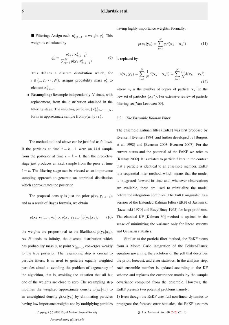
Filtering: Assign each xik|k−1, a weight qik. This

weight is calculated by

qik =p(yk|xik|k−1)∑Nj=1 p(yk|x

jk|k−1)

(9)

This defines a discrete distribution which, for

i ∈ 1, 2, · · · , N, assigns probability mass qik to

element xik|k−1

• Resampling: Resample independently N times, with

replacement, from the distribution obtained in the

filtering stage. The resulting particles, xiki=1,··· ,N ,

form an approximate sample from p(xk|y1:k) .

The method outlined above can be justified as follows.

If the particles at time t = k − 1 were an i.i.d sample

from the posterior at time t = k − 1, then the predictive

stage just produces an i.i.d. sample from the prior at time

t = k. The filtering stage can be viewed as an importance

sampling approach to generate an empirical distribution

which approximates the posterior.

The proposal density is just the prior p(xk|y1:k−1),

and as a result of Bayes formula, we obtain

p(xk|y1:k−1,yk) ∝ p(xk|y1:k−1)p(yk|xk), (10)

the weights are proportional to the likelihood p(yk|xk).

As N tends to infinity, the discrete distribution which

has probability mass qi at point xik|k−1, converges weakly

to the true posterior. The resampling step is crucial to

particle filters. It is used to generate equally weighted

particles aimed at avoiding the problem of degeneracy of

the algorithm, that is, avoiding the situation that all but

one of the weights are close to zero. The resampling step

modifies the weighted approximate density p(xk|yk) to

an unweighted density p(xk|yk) by eliminating particles

having low importance weights and by multiplying particles

having highly importance weights. Formally:

p(xk|yk) =

N∑i=1

qiδ(xk − xki) (11)

is replaced by

p(xk|yk) =

N∑i=1

1

Nδ(xk − xk

?) =

N∑i=1

niNδ(xk − xk

i)

(12)

where ni is the number of copies of particle xki in the

new set of particles xk?. For extensive review of particle

filtering see[Van Leeuwen 09].

3.2. The Ensemble Kalman Filter

The ensemble Kalman filter (EnKF) was first proposed by

Evensen [Evensen 1994] and further developed by [Burgers

et al. 1998] and [Evensen 2003, Evensen 2007]. For the

current status and the potential of the EnKF we refer to

[Kalnay 2009]. It is related to particle filters in the context

that a particle is identical to an ensemble member. EnKF

is a sequential filter method, which means that the model

is integrated forward in time and, whenever observations

are available, these are used to reinitialize the model

before the integration continues. The EnKF originated as a

version of the Extended Kalman Filter (EKF) of Jazwinski

[Jazwinski 1970] and Bucy[Bucy 1965] for large problems.

The classical KF [Kalman 60] method is optimal in the

sense of minimizing the variance only for linear systems

and Gaussian statistics.

Similar to the particle filter method, the EnKF stems

from a Monte Carlo integration of the Fokker-Planck

equation governing the evolution of the pdf that describes

the prior, forecast, and error statistics. In the analysis step,

each ensemble member is updated according to the KF

scheme and replaces the covariance matrix by the sample

covariance computed from the ensemble. However, the

EnKF presents two potential problems namely:

1) Even though the EnKF uses full non-linear dynamics to

propagate the forecast error statistics, the EnKF assumes




that all probability distributions involved are Gaussian.

2) The updated ensemble preserves only the first two

moments of the posterior.

Let p(x) denote the Gaussian prior probability density

distribution of the state vector x with mean µ and covariance

Q

p(x) ∝ exp(−1

2(x− µ)TQ−1(x− µ)

)We assume the data y to have a Gaussian pdf with

covariance R and mean Hx, where H is the so-called the

observation matrix, is related to h of equation (4), and where

the value Hx assumes what the value of the data y would

be in absence of observation errors. Then p(y|x) is the

probability (likelihood) of the observations y given that the

truth is given by the model state x and is of the form

p(y|x) ∝ exp

(−1

2(y −Hx)TR−1(y −Hx)

).

According to the Bayes theorem the posterior probability

density follows from the relation

p(x|y) ∝ p(y|x)p(x). (13)

There are many variants of implementing the EnKF

of various computational efficiency and in what follows

we employ standard formulation of the EnKF for linear

and nonlinear observation operators with covariance

localization. See [Evensen 1994, Burgers et al. 1998,

Mandel 2006, Mandel 2007 and Lewis et al. 2006], also see

[Nerger et al. 2005] and Sakov and Oke [Sakov 2008] The

implementation of the standard EnKF may be divided into

three steps, as follows:

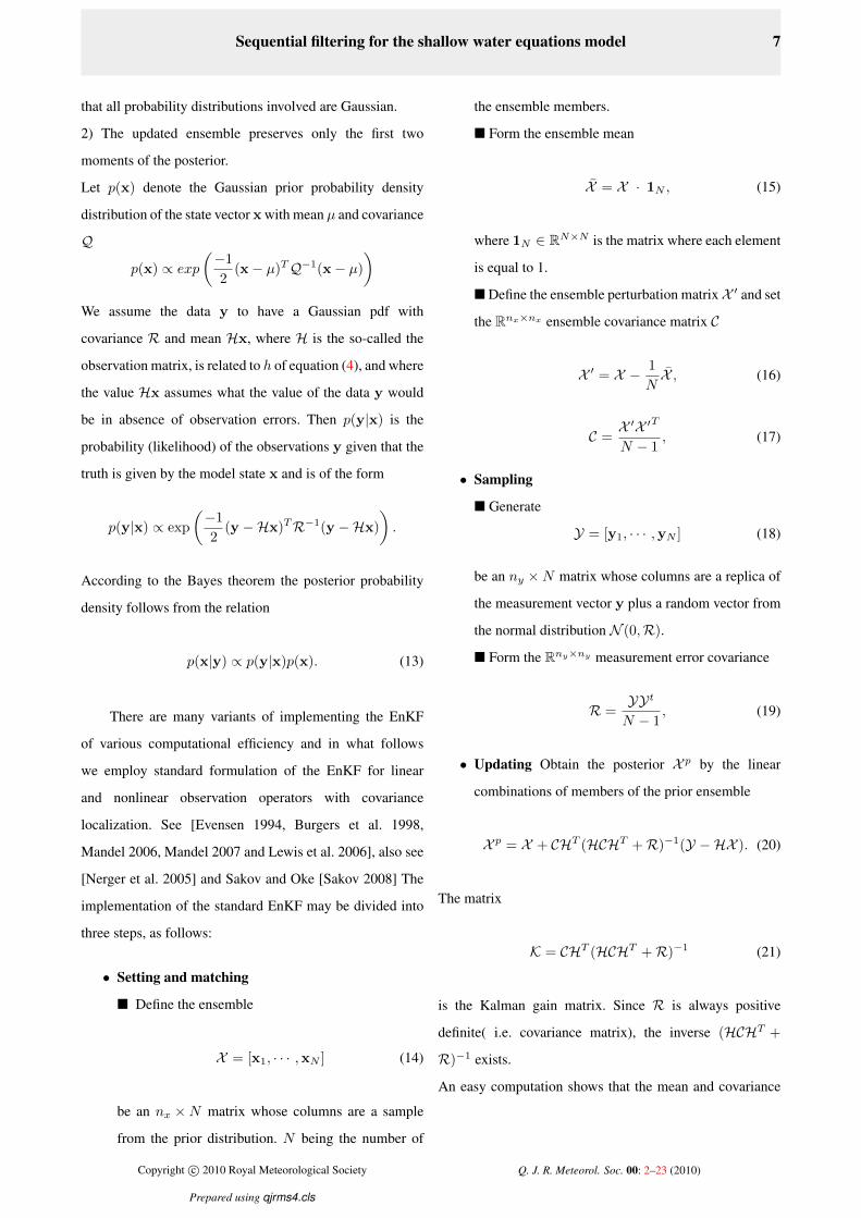
• Setting and matching

Define the ensemble

X = [x1, · · · ,xN ] (14)

be an nx ×N matrix whose columns are a sample

from the prior distribution. N being the number of

the ensemble members.

Form the ensemble mean

X = X · 1N , (15)

where 1N ∈ RN×N is the matrix where each element

is equal to 1.

Define the ensemble perturbation matrixX ′ and set

the Rnx×nx ensemble covariance matrix C

X ′ = X − 1

NX , (16)

C =X ′X ′T

N − 1, (17)

• Sampling

Generate

Y = [y1, · · · ,yN ] (18)

be an ny ×N matrix whose columns are a replica of

the measurement vector y plus a random vector from

the normal distribution N (0,R).

Form the Rny×ny measurement error covariance

R =YYt

N − 1, (19)

• Updating Obtain the posterior X p by the linear

combinations of members of the prior ensemble

X p = X + CHT (HCHT +R)−1(Y −HX ). (20)

The matrix

K = CHT (HCHT +R)−1 (21)

is the Kalman gain matrix. Since R is always positive

definite( i.e. covariance matrix), the inverse (HCHT +

R)−1 exists.

An easy computation shows that the mean and covariance



8 M.Jardak et al.

of the posterior or updated ensemble are given by

X p = X p +K [y − (HX p + d)] , (22)

with the vector d results from the affine measurement

relation

h(x) = Hx + d. (23)

The covariance of the posterior obeys

Cp = C − K[HCHT +R

]KT , (24)

In the case of nonlinear observation operators, a

modification to the above algorithm is advised. As advised

by Evensen [Evensen 2003] and following his notation, let

x the augmented state vector made of the state vector and

the predicted observation vector (nonlinear in this case).

x =

x

H(x)

. (25)

Define the linear observation operator H by

H

x

y

= y (26)

and carry out the steps of the EnKF formulation in

augmented state space x and H instead of x and H.

Superficially, this technique appears to reduce the nonlinear

problem to the previous linear observation operator case.

However, whilst the augmented problem, involving linear

observation problem, is a reasonable way of formulating the

EnKF, it is not as well-founded as the linear case, which can

be justified as an approximation to the exact and optimal KF.

To prevent the occurrence of filter divergence usually

due to the background-error covariance estimates from

small number of ensemble members as pointed out in

[Houtekamer and Mitchell 1998], the use of covariance

localization was suggested. Mathematically, the covariance

localization increases the effective rank of the background

error covariances. See the work of [ Gaspari and

Cohn 1999] also [Hamill and Snyder 2000, 2006] and

[Ehrendorfer 2007]. The covariance localization consists of

multiplying point by point the covariance estimate from

the ensemble with a correlation function that is 1.0 at

the observation location and zero beyond some prescribed

distance. Mathematically, to apply covariance localization,

the Kalman gain

K = CHT (HCHT +R)−1

is replaced by a modified gain

K = [ρ C]HT (H [ρ C]HT +R)−1 (27)

where ρ denotes the Schur product ( The Schur product

of matrices A and B is a matrix D of the same dimension,

where dij = aijbij) of a matrix S with local support with

the covariance model generated by the ensemble. Various

correlation matrices have been used. For the present model,

we used the usual Gaussian correlation function

ρ(D) = exp[−[D

l]2], (28)

where l is the correlation length here l = 200 length units.

In addition, the additive covariance inflation of [Anderson

and Anderson 1999] with the inflation factor r = 1.001 has

been employed.

3.3. The Maximum Likelihood Ensemble Filter

The Maximum Likelihood Ensemble Filter (MLEF)

proposed by Zupanski [Zupanski 2005], and Zupanski and

Zupanski [Zupanski 2006] is a hybrid filter combining

the 3-D variational method with the EnKF. It maximizes

the likelihood of posterior probability distribution which

justifies its name. The method comprises three steps, a

forecast step that is concerned with the evolution of the

forecast error covariances, an analysis step based on solving

a non-linear cost function and an updating step.




• Forecasting:

It consists of evolving the square root analysis

error covariance matrix through the ensembles. The

starting point is from the evolution equation of

the discrete Kalman filter described in Jazwinski

[Jazwinski 1970]

P kf =Mk−1,kPkaMT

k−1,k +Qk−1, (29)

where P (k)f is the forecast error covariance matrix at

time k,Mk−1,k is the linearized forecast model (e.g.,

Jacobian) from time k − 1 to time k, and Qk−1 is the

model error matrix which is assumed to be normally

distributed. Since P k−1a is positive matrix for any k,

equation (29) could be factorized and written as

P kf =

(Pkf )1/2︷︸︸︷(

Mk−1,k(P ka )1/2)(Mk−1,k(P ka )1/2

)T+Qk−1

where (P ka )1/2 is of the form

(P ka )1/2 =

pk(1,1) p

k(2,1) · · · p

k(N,1)

pk(1,2) pk(2,2) · · · p

k(N,2)

pk(1,n) pk(2,n) · · · p

k(N,n)

, (30)

as usual N is the number of ensemble members and

n the number of state variables. The lower case pki,j

are obtained by calculating the square root of (P ka ).

Using equation(30), the square root forecast error

covariance matrix (P kf )1/2 can then be expressed as

(P kf )1/2 =

bk(1,1) b

k(2,1) · · · b

k(N,1)

bk(1,2) bk(2,2) · · · b

k(N,2)

bk(1,n) bk(2,n) · · · b

k(N,n)

, (31)

where for each 1 ≤ i ≤ N

bki =

bk(i,1)

bk(i,2)

...

bk(i,n)

=Mk−1,k

xk1 + pk(i,1)

xk2 + pk(i,2)

...

xkn + pk(i,n)

−

Mk−1,k

xk1

xk2...

xkn

.

The vector xk =(xk1x

k2 · · ·xkn

)Tis the analysis state

from the previous assimilation cycle. which is found

from the posterior analysis pdf as presented in

[Lorenc 1986].

• Analyzing:

The analysis step for the MLEF involves solving

a non-linear minimization problem. As in Lorenc

[Lorenc 1986], the associated cost function is defined

in terms of the forecast error covariance matrix and is

given as

J (x) = 12 (x− xb)

T(P kf

)−1

(x− xb)+

12 [y − h(x)]

T R−1 [y − h(x)]

(32)

where y is the vector of observations, h is the non-

linear observation operator, R is the observational

error covariance matrix and xb is a background state

given by

xb =Mk−1,k(xk) +Qk−1. (33)

Through a Hessian preconditioner we introduce the

change of variable

(x− xb) = (P kf )1/2(I +O)−T/2ξ (34)



10 M.Jardak et al.

where ξ is vector of control variables, O is referred

to as the observation information matrix and I is the

identity matrix. The matrix O is provided by

O = (P kf )T/2HTR−1H(P kf )T/2 =

(R−1/2H(P kf )1/2)T (R−1/2H(P kf )1/2)

here H is the Jacobian matrix of the non-linear

observation operator h evaluated at the background

state xb.

Let Z the matrix defined by

Z =

z(1,1) z(2,1) · · · z(N,1)

z(1,2) z(2,2) · · · z(N,2)

z(1,n) z(2,n) · · · z(N,n)

,

and let zi assumes the form

zi =

z(i,1)

z(i,2)

...

z(i,n)

= R−1/2Hbki .

From the following approximations

zi ≈ R−1/2[h(x + bki )− h(x)

], (35)

and

O ≈ ZZT . (36)

one can use an eigenvalue decomposition of the

of symmetric positive definite matrix I +O to

calculate the inverse square root matrix necessary to

the updating step. It is worth mentioning that the

approximation (35) is not necessary and a derivation

of the MLEF not involving (35) has been recently

developed in Zupanski et al. [Zupanski 08]

• Updating:

The final point about MLEF is to update the square

root analysis error covariance matrix. In order to

estimate the analysis error covariance at the optimal

point, the optimal state xopt minimizing the cost

function J given by (32)is substituted

(P ka )T/2 = (P kf )T/2(I +O(xopt))−T/2. (37)

4. Numerical results

4.1. Model set-up

As in [Williamson 1992,1997,2007] and [Jakob et al. 1995],

the grid representation for any arbitrary variable φ is related

to the following spectral decomposition

φ(λ, µ) =

M∑m=−M

N(m)∑n=|m|

φm,nPm,n(µ)eimλ, (38)

where Pm,n(µ)eimλ are the spherical harmonic functions

[Boyd 01]. Pm,n(µ) stands for the Legendre polynomial.M

is the highest Fourier wavenumber included in the east-west

representation, N(m) is the highest degree of the associated

Legendre polynomials for longitudinal wavenumber m.

The coefficients of the spectral representation (38) are

determined by

φm,n =

∫ 1

−1

1

2π

∫ 2π

0

φ(λ, µ)e−imλPm,n(µ)dλdµ (39)

The inner integral represents a Fourier transform,

φm(µ) =1

2π

∫ 2π

0

φ(λ, µ)e−imλdλ (40)

which is evaluated using a fast Fourier transform routine.

The outer integer is evaluated using Gaussian quadrature on

the transform grid.

φm,n =

J∑j=1

φm(µ)Pm,n(µ)ωj , (41)




where µj denotes the Gaussian grid points in the meridional

direction and ωj is the Gaussian weight at point µj .

The meridional grid points are located at the Gaussian

latitudes θj , which are the J roots of the Legendre

polynomial Pj(sin θj) = 0. The number of grid points in

the longitudinal and meridional directions are determined so

as to allow the unaliased representation of quadratic terms,

I ≥ 3M + 1

J ≥ 3N + 1

2

where N is the highest wavenumber retained in the

latitudinal Legendre representation N = maxN(m) = M .

The pseudo spectral method, also known as the spectral

transform method in the geophysical community, of [Orszag

1969, 1970] and [Eliassen et al. 1970] has been used to

tackle the nonlinearity.

In conjunction with the spatial discretization described

before, the time discretization, two semi-implicit time

steps have been used for the initialization. Because of the

hyperbolic type of the shallow water equations, the centered

leapfrog scheme

φk+1m,n − φk−1

m,n

2∆t= F(φkm,n) (42)

has been invoked for the subsequent time steps. After

the leapfrog time-differencing scheme is used to obtain

the solution at t = (k + 1)∆t, a slight time smoothing is

applied to the solution at time k∆t (Asselin filter) .

φkm,n = φkm,n + α[φk+1m,n − 2φkm,n + φk−1

m,n

](43)

replacing the solution at time k. It reduces the amplitude of

different frequencies ν by a factor 1− 4α sin2(ν∆t2 ).

4.2. EnKF set-up and numerical results

In all our numerical experiments a time step of ∆t = 600

sec has been employed. The observations were provided at a

frequency consisting of one set of observations every 36∆t.

4.2.1. Impact of the number of observations and the

number of ensemble members

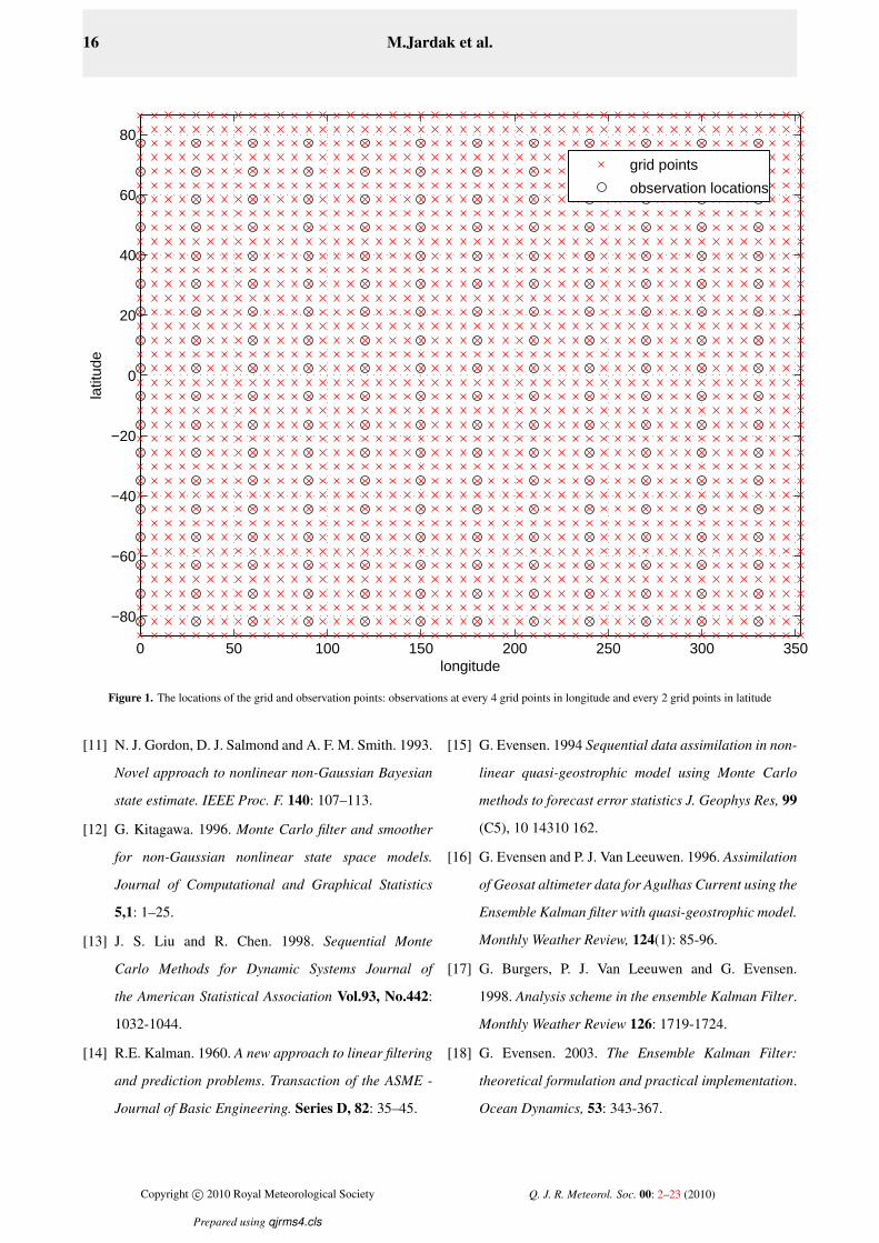
The impact of the number of observations follows the

findings of [ Fletcher and Zupanski 2008]. In fact after

attaining a number of observations threshold, all the root

mean square errors rmses for all the fields ( namely the

components of the velocity and geopotential) coincide. In

our test the number of the observations threshold was

attained at around 912 observations at each observation

time. The observational grid is a subset of the rhomboidal

spectral truncation (48x38) and consists of observations

being distributed at every grid point in the longitude and

every 2 points in the latitude, as presented in figure 1.

The impact of the number of ensemble members on

the results has also been examined. We have conducted

several experiments with different numbers of ensemble

members, namely, 50, 100, 200 and 300 ensemble members,

respectively. Our results reveal that employing only 100

ensemble members was sufficient to successfully perform

the data assimilation and that using higher number of

ensemble members had no impact on the ensuing results.

4.2.2. Linear observation operator case - description of

the EnKF results

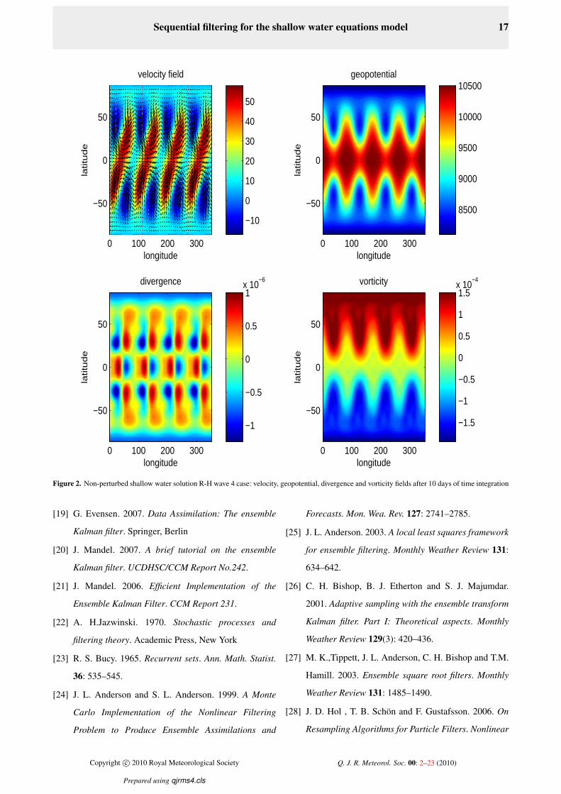
Figure 2 provides an overview of the unperturbed shallow

water solution using the Rossby-Haurwitz wave no.4 as

initial conditions after 10 days of time integration.

In figure 3 we present a 1% random perturbation

around the mean of the geopotential field. This perturbed

field along with the perturbed velocity divergence and vor-

ticity fields will serve as initialization for the observations.

In figure 4 we present an overview of the results

obtained using 10 days EnKF data assimilation time



12 M.Jardak et al.

integration. The linear observation operator H(u) = u has

been employed, 100 ensemble members were used with 1%

random perturbation around the mean accounting for the

standard deviation for the model error covariance matrix.

In the presence of 1% and 3% random perturbations

around the mean respectively, the RH wave no. 4 test

case preserves its global characteristic shape for more than

30 days of data assimilation time integration. This shows

the resilience of the RH wave no. 4 test case to random

perturbation in the presence of linear observation operator.

4.2.3. Nonlinear observation operator case - description

of the EnKF results

Here we are employing H(u) = u2 as a representative of

a nonlinear observation operator ( we have also tested

H(u) = u4 results not shown) The number of observation

points is 912 ( their distribution in space and time being

identical to the linear observation operator EnKF case).

The EnKF for the nonlinear observation operator H(u) =

u2 starts to manifest a deterioration at a round 5 days

of data assimilation time integration. By 10 days of data

assimilation time integration a full filter divergence takes

place as it can be seen in the rmses as well as in the

corresponding Talagrand diagram. Figure 5 displays the

corresponding Talagrand diagram also known as the rank

score. Contrary to the linear observation operator Talagrand

diagram where a uniform ensemble repartition is observed,

the Talagrand diagram for the nonlinear case displays a

tendency to a weakly U-shaped ensemble repartition. This

result characterizes the onset of filter divergence. In figure

6 we present the true, the EnKF analysis for one ensemble

member and the expected analysis geopotential fields for

5 days data assimilation time integration. This illustration

confirms the validity of the Talagrand diagram. As a matter

of fact, a deterioration of the typical shape of the RH wave

no.4 test case is noticeable.

Figure 7 regroups the Talagrand diagrams and root

mean square errors rmses corresponding to different values

of the random perturbation around the mean, namely

1%, 3% and 6% perturbations. The Talagrand diagrams

display now a non symmetrical U shape characteristic of

filter divergence as well as bias. An increase in the values

of the frequencies follows the increase in the perturbation

percentage. The rmses of the geopotential field, presented in

the same figure, increase accordingly with the perturbation.

In figures 8 and 9 we present the true, the EnKF

analysis for one ensemble member and the expected

analysis geopotential forecast and analysis geopotential

fields for 10 days EnKF window of data assimilation

with 1% and 3% perturbation around the mean. The

same nonlinear observation operator H(u) = u2 has been

employed. The results obtained point to a total loss of shape

and symmetry deterioration of the RH wave no. 4 test case.

The purpose of the this section is not to establish the

onset of filter divergence, rather to show that the fixture

of Evenson [Evenson 2003] is not suitable for nonlinear

observation operator. New efforts to mitigate the problem

of high nonlinearity in EnKF have been undertaken. The

recent work of Kalnay and collaborators, [Kalnay priv.

comm. 2008], [Kalnay and Yang 2008] and [Kalnay and

Yang 2010] suggests an approach involving outer loops of

minimization, borrowed from variational data assimilation

practice. They introduce an empirical convergence criterion

within a nonstandard iterative minimization scheme.

Common to both mentioned algorithms is that they treat

each iteration of minimization as a quadratic sub-problem

and thus rely on the use of traditional Kalman filter linear

analysis update equation in each iteration.

4.3. PF set-up and numerical results

As in the previous (EnKF) section, all our numerical

experiments employ a time step of ∆t = 600sec. The

observations are sampled once every 6 hours i.e. at a

frequency consisting of one observation every 36 time steps.




4.3.1. The impact of number of particles and of the

resampling strategy

In view of recent results in the literature ( such as

[Van Leeuwen 2009] [Snyder et al. 2008] ) the issue of

choice of an adequate number of particles is of paramount

importance. In order to avoid filter degeneracy we follow

the suggestion of Van-Leeuwen [Van Leeuwen 2009] as

to the choice of suitable number of particles, that should

be not smaller than the number of degrees of freedom of

the simulated system. We tested three cases namely, 1000,

1500 and 1900 particle filters (compare to 48× 38 modes

in the latitude-longitude directions for the spherical-spectral

shallow-water model )

In as far as PF resampling methods are concerned,

we tested three resampling techniques namely, residual,

systematic and multinomial resampling,respectively. All

of them performed equally well with a slight edge

to the systematic resampling technique in as far as

computational efficiency is concerned see [Doucet et al.

2001, Arulampalam et al. 2002 and Van Leeuwen 2009]. A

novel feature introduced here is the equivalent of Talagrand

diagrams, where instead of taking the ensemble members

we took the particles. Then we iterated over the number

of bins (1900 particles, 51 bins). Similar to the ensemble

framework, this diagram could be a good tool to detect

systematic flaws of a particle filter prediction system.

4.3.2. Linear observation operator case

The linear observation operator assuming the formH(u) =

u has been employed for the particle filter case and we do

not show the related results. However, we observe almost

identical results to those obtained for the EnKF linear

observation operator case, in fact the R-H wave no 4 test

case preserves its global characteristic shapes with minor

changes occurring in the center of the recirculation zones at

around 10 days of data assimilation time integration.

4.3.3. Non-linear observation operator case

We consider the impact of nonlinear observation operator

for the particle filter (PF) when H(u) = u2. As displayed

in figure 10, where the true, PF analysis for one particle

geopotential fields for 1% and 3% perturbation around

the mean are depicted. After 10 days data assimilation

time integration,the R-H wave no 4 test case preserves

its global characteristic shape and no distortion nor cell

pattern breakdown can be detected. These results should be

contrasted to our EnKF findings of filter divergence for the

same data assimilation time integration.

A part from the bias ( i.e. the first and last bins) of

the U-shaped diagrams shown in figure 11, we have

uniformity of the frequencies repartition indicates that the

probability distribution has been well sampled. In fig 12

we present the time evolution of the rmses after 10 days

of data assimilation time integration of PF for 1% and

3% perturbation around the mean. The striking result is

that the rmses variation is now bounded in contrast to the

EnKf case where the increase in the corresponding rmses

is quasi-exponential. The effect of degree of nonlinearity

of the observation operator in the PF case has been also

examined. As figure 13 shows that a stronger nonlinearity

(i.eH(u) = exp(u) ) has no substantial effect on the rmses.

Indeed, the rmses envelope is not affected despite presence

of oscillations characteristic of the PF filter.

4.4. MLEF set-up and results

Only 30 ensemble members were sufficient for carrying

out the MLEF runs, while the number of cycles was set to

70. The iterative nonlinear minimization method employed

for cost function minimization was the Flecher-Reeves

nonlinear conjugate gradient algorithm. In each of the

MLEF data assimilation cycles, 5 iterations are performed

to obtain the analysis. The standard deviation of each of the

Gaussian state and observation noise was taken to be 1%

random perturbation around the mean. No localization nor

inflation were used within the ensemble part of this method.



14 M.Jardak et al.

We observe similar results to those obtained for the

EnKF and PF in linear observation operator case, namely

that the global characteristic shapes of the filtered solution

are preserved. This feature is presented in figure

When H(u) = u2, we observe additional aspects in

the divergence and the vorticity fields as it can be seen

in figure after 10 days of model integration with data

assimilation. The striking resemblance between the PF and

MLEF results manifests the successful implementation of

both filters. This result is further confirmed as the degree

of nonlinearity of the observation operators was increased

fromH(u) = u2 toH(u) = eu. Our numerical experiments

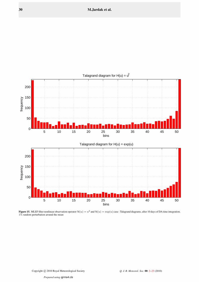
are presented in in figure 14. As presented in figure 15,

we observe that a part from the bias ( i.e. the first and last

bins) of the U-shaped diagrams shown ,we have uniformity

of the frequencies repartition indicates that the probability

distribution has been well sampled. This is in agreement

with our PF findings. The rmses presented in figure 16 are

bounded and the nonlinearity of the observation operator

has no effect on the rmses, consequently the MLEF filter

predicts well the true solution independently of the linearity

of the observation operator.

5. Summary and conclusions

In this paper, a comparison was carried out for the three

most popular ensemble data assimilation methods (EnsDA)

for a spherical nonlinear shallow water equations model

discretized via a spectral model and tested for the Rossby

Haurwitz wave no. 4.

The Monte Carlo version of EnKF, the particle filter PF with

several resampling strategies and finally as a representative

of hybrid filters, the maximum likelihood filter MLEF were

tested in the presence of both linear and highly nonlinear

observation operators. The nonlinear observation operators

replicate and stand as a proxy for more realistic processes

such as cloud, aerosol and precipitation processes, as well

as remote sensing (e.g., satellite and radar) observations.

While the typical EnsDA analysis equation assumes

linearity and Gaussianity for EnKF, (thus fundamentally

preventing this EnsDA from extracting maximum

information from nonlinear observations) we have also

tested a Bayesian filter, the particle filter, whose analysis

equation is nonlinear as well as the MLEF hybrid filter,

which accommodates nonlinear observation operators as

well as non-Gaussianity.

In the case of linear observation operator results for the

three above mentioned sequential data assimilation filters

leads to the conclusion, that the aforementioned methods

are comparable and yield satisfactory results. Amongst the

different error metrics used to assess filter divergence, we

chose to retain the Talgrand diagram (known also as Rank

Score) , the usual rmse statistics. Results of Talagrand

diagram for EnKF in the presence of nonlinear operators

show that filter divergence onset occurs at about 5 days of

data assimilation using the R-H wave no.4 test case. We

conclude that EnKF with Evensen’s fixture for nonlinearity

fails to converge for nonlinear observation operators . In

contrast the other two filters (PF and MLEF) handled well

the issue of nonlinearity of the observation operators as well

as non-Gaussianity, as expected. The three error metrics

retained support the results obtained.

These results are of course a function of our particular

implementation of the EnKF, PF and MLEF, respectively

and are a function of the number of particles (number of

ensemble members) the number of observations as well

as the particular model tested. In as far as computational

efficiency, the MLEF was found to be faster than the EnKF,

while the PF filter proved to be the most time consuming in

as far as the shallow water equations model with nonlinear

observation operator is concerned.

The EnKF version for the nonlinear observation oper-

ator H(u) = u2 is displaying a significant discrepancy

between the true and filtered EnKF solutions. is consid-

erable. We join here many authors, [Jardak et al. 2010],

[Nakano et al. 2007] and [Apte et al. 2008A,2008B] to

cite but a few, to draw the conclusion that even with

the modification suggested by [Evensen 2003], the EnKF




filter diverges in the case of nonlinear observation oper-

ator applied here to the shallow water equations model.

In conclusion, we can only compare between the PF and

the MLEF filters in the presence of nonlinear observation

operators. Both the PF and the MLEF filters exhibit good

performance in terms of results of sequential data assimi-

lation as evidenced by the rmses and the divergence statis-

tics. for the tests conducted with the nonlinear observation

operators the MLEF method appears to have an edge in

terms of CPU time over the PF method method with SR

resampling. Indeed, the PF results were obtained using

1000-1900 particles, while MLEF obtained similar results

for only 30-300 ensembles.

Acknowledgements

The research of Prof. I.M. Navon and Dr. M. Jardak was

supported by the National Science Foundation (NSF), grant

ATM-03727818. The authors also acknowledge the support

by NASA Modeling, Analysis, and Prediction Program

under Award NNG06GC67G. Prof. Navon acknowledges

the National Science Foundation (NSF), grant ATM-

0931198. Dr. Zupanski acknowledges the National Science

Foundation (NSF), grant ATM-0930265. Finally, Dr.

Jardak is grateful to W.H.Hanya and M.O.Nefysa for the

continuous help.

References

[1] D. L. Williamson, J. B. Drake, J. J. Hack, R. Jacob

and P. N. Swarztrauber.1992. A standard test set for

numerical approximations to shallow-water equations

in spherical geometry. J. Comput. Phys 102: 211–224.

[2] D. L. Williamson. 1997. Climate Simulations with

a spectral semi-Lagrangian model with linear

grid,” Numerical Methods in Atmospheric and

Ocean Modelling. Canadian Meteorological and

Oceanographic Society 279–292.

[3] D. L. Williamson. 2007. The Evolution of Dynamical

Cores for Global Atmospheric Models. Journal of the

Meteorological Society of Japan 85B: 241–269.

[4] R. Jakob-Chien, J. J. Hack and D. L. Williamson.1995.

Spectral transform solutions to the shallow water test

set. J. Comput. Phys 119: 164–187 .

[5] J. P. Boyd , 2001. Chebyshev and Fourier Spectral

Methods, Second Edition (Revised). Dover Publishing

[6] M. L. Berliner and C. K. Wikle. 2007. A Bayesian

tutorial for data assimilation. Physica D. 30: 1–16.

[7] M. L. Berliner and C. K. Wikle. 2007. Approximate

importance sampling Monte Carlo for data assimila-

tion. Physica D. 30: 37-49

[8] A. Doucet, A. , S. Godsill, S. and C. Andrieu. 2000.

On Sequential Monte Carlo sampling methods for

Bayesian filtering. Statistics and Computing. 10 (3):

197–208.

[9] A. Doucet, J. F. G. de Freitas and N. J. Gordon. 2001.

An introduction to sequential Monte Carlo methods.

Sequential Monte Carlo Methods in Practice, Doucet,

A. , de Freitas, J.F.G and Gordon, N.J (eds.) Springer-

Verlag, New York

[10] M. S. Arulampalam, S. Maskell, N. Gordon and

T. Clapp. 2002. A Tutorial on Particle Filters for

Online Nonlinear/Non-Gaussian Bayesian Tracking.

IEEE transactions on signal processing. Vol(150)

no.2: 174–188.



16 M.Jardak et al.

0 50 100 150 200 250 300 350

−80

−60

−40

−20

0

20

40

60

80

longitude

latit

ude

grid points

observation locations

Figure 1. The locations of the grid and observation points: observations at every 4 grid points in longitude and every 2 grid points in latitude

[11] N. J. Gordon, D. J. Salmond and A. F. M. Smith. 1993.

Novel approach to nonlinear non-Gaussian Bayesian

state estimate. IEEE Proc. F. 140: 107–113.

[12] G. Kitagawa. 1996. Monte Carlo filter and smoother

for non-Gaussian nonlinear state space models.

Journal of Computational and Graphical Statistics

5,1: 1–25.

[13] J. S. Liu and R. Chen. 1998. Sequential Monte

Carlo Methods for Dynamic Systems Journal of

the American Statistical Association Vol.93, No.442:

1032-1044.

[14] R.E. Kalman. 1960. A new approach to linear filtering

and prediction problems. Transaction of the ASME -

Journal of Basic Engineering. Series D, 82: 35–45.

[15] G. Evensen. 1994 Sequential data assimilation in non-

linear quasi-geostrophic model using Monte Carlo

methods to forecast error statistics J. Geophys Res, 99

(C5), 10 14310 162.

[16] G. Evensen and P. J. Van Leeuwen. 1996. Assimilation

of Geosat altimeter data for Agulhas Current using the

Ensemble Kalman filter with quasi-geostrophic model.

Monthly Weather Review, 124(1): 85-96.

[17] G. Burgers, P. J. Van Leeuwen and G. Evensen.

1998. Analysis scheme in the ensemble Kalman Filter.

Monthly Weather Review 126: 1719-1724.

[18] G. Evensen. 2003. The Ensemble Kalman Filter:

theoretical formulation and practical implementation.

Ocean Dynamics, 53: 343-367.




0 100 200 300

−50

0

50

longitude

latitu

de

velocity field

−10

0

10

20

30

40

50

longitude

latitu

de

geopotential

0 100 200 300

−50

0

50

8500

9000

9500

10000

10500

longitude

latitu

de

divergence

0 100 200 300

−50

0

50

−1

−0.5

0

0.5

1x 10

−6

longitude

latitu

de

vorticity

0 100 200 300

−50

0

50

−1.5

−1

−0.5

0

0.5

1

1.5x 10

−4

Figure 2. Non-perturbed shallow water solution R-H wave 4 case: velocity, geopotential, divergence and vorticity fields after 10 days of time integration

[19] G. Evensen. 2007. Data Assimilation: The ensemble

Kalman filter. Springer, Berlin

[20] J. Mandel. 2007. A brief tutorial on the ensemble

Kalman filter. UCDHSC/CCM Report No.242.

[21] J. Mandel. 2006. Efficient Implementation of the

Ensemble Kalman Filter. CCM Report 231.

[22] A. H.Jazwinski. 1970. Stochastic processes and

filtering theory. Academic Press, New York

[23] R. S. Bucy. 1965. Recurrent sets. Ann. Math. Statist.

36: 535–545.

[24] J. L. Anderson and S. L. Anderson. 1999. A Monte

Carlo Implementation of the Nonlinear Filtering

Problem to Produce Ensemble Assimilations and

Forecasts. Mon. Wea. Rev. 127: 2741–2785.

[25] J. L. Anderson. 2003. A local least squares framework

for ensemble filtering. Monthly Weather Review 131:

634–642.

[26] C. H. Bishop, B. J. Etherton and S. J. Majumdar.

2001. Adaptive sampling with the ensemble transform

Kalman filter. Part I: Theoretical aspects. Monthly

Weather Review 129(3): 420–436.

[27] M. K.,Tippett, J. L. Anderson, C. H. Bishop and T.M.

Hamill. 2003. Ensemble square root filters. Monthly

Weather Review 131: 1485–1490.

[28] J. D. Hol , T. B. Schon and F. Gustafsson. 2006. On

Resampling Algorithms for Particle Filters. Nonlinear



18 M.Jardak et al.

longitude

latit

ude

0 50 100 150 200 250 300 350

−80

−60

−40

−20

0

20

40

60

80

8000

8500

9000

9500

10000

10500

Figure 3. EnKF filter linear observation operator case : initial perturbation geopotential field

Statistical Signal Processing Workshop, Cambridge,

United Kingdom.

[29] N. Metropolis, and S. Ulam. 1944. The Monte Carlo

Method. J. Amer. Stat. Assoc. 44: 335–341.

[30] J. L. Lewis, S. Lakshivarahan and S. K. Dhall.

2006. Dynamic Data Assimilation: A least squares

approach. Cambridge University Press, in the series

on Encyclopedia of Mathematics and its Applications

Volume 104

[31] E. N. Lorenz. 1963. Deterministic nonperiodic flow. J.

Atmos. Sci., 20:130–141 .

[32] E. N. Lorenz. 1969. The predictability of a flow which

possesses many scales of motion. Tellus 21: 289–307.

[33] S. E. Cohn. 1997. An introduction to estimation

theory. Journal of the Meteorological Society of Japan

Vol.75, No.1B 257–288

[34] X. Xiong, I. M. Navon and B. Uzunoglu. 2006. A

Note on the Particle Filter with Posterior Gaussian

Resampling Tellus 58A: 456–460.

[35] P. Houtekamer and H. Mitchell. 1998. Data assimila-

tion using an ensemble Kalman filter technique.Mon.

Wea. Rev. 126: 796–811.

[36] P. L. Houtekamer and H. L. Mitchell. 2001. A

Sequential Ensemble Kalman Filter for Atmospheric

Data Assimilation. Mon.Wea.Rev.129: 123–137.

[37] P. L. Houtekamer, H. L. Mitchell, G. Pellerin, M.

Buehner, M. Charron, L. Spacek and B. Hansen. 2005.




0 100 200 300

−50

0

50

longitude

latit

ude

velocity field

−20

0

20

40

60

longitude

latit

ude

geopotential

0 100 200 300

−50

0

50

8500

9000

9500

10000

10500

longitude

latit

ude

divergence

0 100 200 300

−50

0

50

−8

−6

−4

−2

0

2

4

6

x 10−6

longitude

latit

ude

vorticity

0 100 200 300

−50

0

50

−1.5

−1

−0.5

0

0.5

1

1.5x 10

−4

Figure 4. EnKF filter linear observation operator case : velocity, geopotential, divergence and vorticity fields after 10 days of DA time integration. 100ensemble members and 1% random perturbation around the mean

A Sequential Ensemble Kalman Filter for Atmospheric

Data Assimilation Mon.Wea.Rev.133: 604–620.

[38] S. L. Dance. 2004. Issues in high resolution limited

area data assimilation for quantitative precipitation

forecasting. Physica D 196: 1–27.

[39] G. Kotecha and P. M. Djuric. 2003. Gaussian particle

filtering IEEE Trans. Signal Processing 51: 2592–

2601.

[40] D. E. Goldberg. 1989. Genetic algorithms in search,

optimization and machine learning Addison-Wesley,

Reading.

[41] B. W. Silverman. 1986. Density Estimation for

Statistics and Data Analysis. Chapman and Hall

[42] T. Bengtsson, P. Bickel, and B. Li. 2008. Curse-of-

dimensionality revisited:Collapse of the particle filter

in very large scale systems. Probability and Statistics:

Essays in Honor of David A. Freedman Vol. 2, 316–

334 .

[43] P. Bickel, B. Li and T. Bengtsson. 2008. Sharp

Failure Rates for the Bootstrap Particle Filter in High

Dimensions. IMS Collections: Pushing the Limits of

Contemporary Statistics: Contributions in Honor of

Jayanta K. Ghosh Vol.3: 318-329 .

[44] C. Snyder, T. Bengtsson, P. Bickel, and J.L. Anderson.

2008 Obstacles to high-dimensional particle filtering

Mon. Wea. Rev. Vol 136, No12 ,4629–4640.



20 M.Jardak et al.

5 10 15 20 25 30 35 40 45 500

50

100

150

200

bins

freq

uenc

y

Talagrand diagram

0 0.5 1 1.5 2 2.5 3 3.5 4 4.5 5300

320

340

360

380rm

seφ

time(days)

Figure 5. EnKF filter non-linear observation operator caseH(u) = u2: time evolution of the geopotential rmse and Talagrand diagram after 5 days dataassimilation of time integration

[45] D. Zupanski. 1997. A general weak constraint

applicable to operational 4DVAR data assimilation

systems. Mon.Wea.Rev. 125: 2274-2292

[46] M. Zupanski. 2005. Maximum Likelihood Ensemble

Filter. Part 1: the theoretical aspect. Mon.Wea.Rev.

133: 1710–1726.

[47] D. Zupanski, M. Zupanski. 2006. Model error

estimation employing ensemble data assimilation

approach Mon.Wea.Rev. 134: 137–1354.

[48] M. Zupanski, I. M. Navon and D. Zupanski. 2008.

The Maximum Likelihood Ensemble Filter as a

non-differentiable minumization algorithm Q.J.Roy.

Meteor.Soc. 134: 1039–1050

[49] M. Jardak, I. M. Navon and M. Zupanski. 2010.

Comparison of Sequential data assimilation methods

for the Kuramoto-Sivashinsky equation. International

Journal for Numerical Methods in Fluids 136 Issue 4,

374–402

[50] A. C. Lorenc. 1986. Analysis methods for numerical

weather prediction Q. J. Roy. Meteor. Soc. 112: 1177-

1194 .

[51] T. M. Hamill, J. S. Whitaker and C. Snyder. 2001.

Distance-Dependent Filtering of Background Error

Covariance Estimates in an Ensemble Kalman Filter

Mon.Wea.Rev.,129: 2776–2790 .

[52] T. M. Hamill and C. Snyder. 2000. A Hybrid

Ensemble Kalman Filter-3D Variational Analysis

Scheme. Mon.Wea.Rev.128: 2905–2919 .

[53] T. M. Hamill. 2006. Ensemble-based atmospheric

data assimilation. Predictability of Weather and




longitude

latit

ude

true

0 50 100 150 200 250 300 350

−50

0

50

8000

9000

10000

longitude

latit

ude

EnkF analysis geopotential field for one ensemble member

0 50 100 150 200 250 300 350

−50

0

50

8000

9000

10000

longitude

latit

ude

EnKF expected analysis geopotential field

0 50 100 150 200 250 300 350

−50

0

50

8000

9000

10000

Figure 6. EnKF filter non-linear observation operator case H(u) = u2: true, the EnKF analysis for one ensemble member and the expected analysisgeopotential fields after 5 days of data assimilation time integration. 100 ensemble members and 1% random perturbation around the mean

Climate, Cambridge Press, 124–156 .

[54] T.M. Hamill. 2001. Interpretation of rank histogram

for verifying ensemble forecasts. Mon. Weather Rev.

129(3): 550–560

[55] L. Nerger, ,W. Hiller, J. Schrater. 2005. A comparison

of error subspace Kalman filters. Tellus A,57 (5): 715–

735

[56] G. Gaspari, S. E. Cohn. 1999. Construction of

correlation functions in two and three dimensions. Q.

J. Roy. Meteor Soc. Vol 125 Issue 554:723-757 .

[57] S. Nakano, G. Ueno and T. Higuchi T. 2007. Merging

particle filter for sequential data assimilation.

Nonlinear Processes in Geophysics 14: 395409

[58] A. Apte , C. K. R. T. Jones, A. M. Stuart and J. Voss.

2008. Data assimilation: Mathematical and statistical

perspectives. Int. J. Numer. Meth. Fluids 56: 1033–

1046

[59] A. Apte , C. K. R. T. Jones and A. M. Stuart. 2008.

Bayesian approach to Lagrangian data assimilation.

Tellus A,60: 336–347

[60] R. K. Smith and D. G. Dritschel. 2006. Revisiting

the Rossby–Haurwitz wave test case with contour

advection. Journal of Computational Physics 217,

Issue 2, 473–484

[61] P. J. van Leeuwen. 2009. Particle filtering in

geophysical systems. Mon.Wea.Rev. 137: Issue 12,

4089–4114

[62] E. Kalnay. 2010 Ensemble Kalman Filter: Current

Status and Potential Data Assimilation: Making Sense

of Observations William Lahoz, Boris Khattatov,



22 M.Jardak et al.

10 20 30 40 500

100

200

300

400

500

bins

freq

uenc

y

Talagrand diagram for 1% perturbation

10 20 30 40 500

50

100

150

200

250

300

350

bins

freq

uenc

y


10 20 30 40 500

50

100

150

bins

freq

uenc

y


0 2 4 6 8 100

200

400

600

800

1000

time(days)

rmse

φ

1% perturbation3% perturbation6% perturbation

Figure 7. EnKF filter non-linear observation operator caseH(u) = u2 and for different random perturabtion around the mean: Talagrand diagrams andtime evolution of root mean square error for the geopotential field for 10 days of time integration

Richard Menard (Editors) Springer

[63] P. Sakov and P. Oke. 2008. Implications of the Form of

the Ensemble Transformation in the Ensemble Square

Root Filters.Mon.Wea.Rev.136: 1042–1052

[64] B. Haurwitz. 1940. The motion of atmospheric

disturbances on the spherical earth. J. Mar. Res. 3

254–267

[65] J. Thuburn and Y. Li. 2000. Numerical simulations of

Rossby-Haurwitz waves. Tellus A 52 (2): 181–189

[66] B. J. Hoskins. 1973. Stability of the Rossby-Haurwitz

wave. Quart. J. Roy. Meteorol. Soc.99: 723–745

[67] N.A. Phillips. 1959. Numerical integration of the

primitive equations on the hemisphere. Mon. Wea.

Rev.87: 333–345

[68] C. G. Rossby and collaborators. 1939. Relation

between variations in the intensity of the zonal

circulation of the atmosphere and the displacements of

the semi-permanent centres of action. J. Marine Res.

2: 38–55

[69] C. A. Pires, O. Talagrand and M. Bocquet. 2010. Diag-

nosis and impacts of non-Gaussianity of innovations

in data assimilation. Physica D 239: 1701–1717

[70] M. Bocquet. 2008. Issues of nonlinearity and non-

gaussianity Contribution to the WWRP/THORPEX.

workshop on 4D-Var and ensemble Kalman filter

inter-comparisons Buenos Aires

[71] A.H. Murphy. 1973. A New Vector Partition of the

Probability Score. Journal of Applied Meteorology




longitude

latit

ude

true

0 50 100 150 200 250 300 350

−50

0

50

longitude

latit

ude

One ensemble member of the EnKF analysis

0 50 100 150 200 250 300 350

−50

0

50

longitude

latit

ude

Expected EnKF analysis

0 50 100 150 200 250 300 350

−50

0

50

8000

9000

10000

8000

9000

10000

8000

9000

10000

Figure 8. EnKF filter non-linear observation operator case H(u) = u2: true, the EnKF analysis for one ensemble member and the expected analysisgeopotential fields after 10 days of data assimilation time integration, 100 ensemble members and 1% random perturbation around the mean

vol. 12, Issue 4: 595–600

[72] A.H. Murphy. 1973. What is a good forecast? An essay

on the nature of goodness in weather forecasting.

Weather and forecasting. 8: 281–293

[73] D.S. Wilks. 1995. Statistical Methods in the Atmos-

pheric Sciences. Academic Press, New York

[74] O. Talagrand, R. Vautard, and B. Strauss. 1997. Evalu-

ation of probabilistic prediction systems. Proceedings,

ECMWF Workshop on Predictability. ECMWF. 1–25

[75] E. Kalnay and S. C Yang. 2010. Accelerating the

spin-up of Ensemble Kalman Filtering. Quart. J. Roy.

Meteor. Soc. in press

[76] J. Diard, P. Bessiere and E. Mazer. 2003. A survey of

probabilistic models, using the bayesian programming

methodology as unifying framework. The second Inter-

national Conference on Computational Intelligence,

Robotics and Autonomous Systems, Singapore

[77] O. Cappe, S.J. Godsill and E. Moulines. 2007. An

Overview of Existing Methods and Recent Advances

in Sequential Monte Carlo. Proceedings of the IEEE

95: 899–924

[78] A.M Stuart. 2010. Inverse Problems: A Bayesian

Prespective. Acta Numerica Vol 19: 451–559



24 M.Jardak et al.

longitude

latit

ude

true

0 50 100 150 200 250 300 350

−50

0

50

8000

9000

10000

longitude

latit

ude

One ensemble member of the EnKF analysis

0 50 100 150 200 250 300 350

−50

0

50

8000

9000

10000

longitude

latit

ude

Expected EnKF analysis

0 50 100 150 200 250 300 350

−50

0

50

8000

9000

10000

Figure 9. EnKF filter non-linear observation operator case H(u) = u2: true, the EnKF analysis for one ensemble member and the expected analysisgeopotential fields after 10 days of data assimilation time integration, 100 ensemble members and 3% random perturbation around the mean




longitude

latit

ude

true geopotential field

0 50 100 150 200 250 300 350

−50

0

50

8000

9000

10000

longitude

latit

ude

PF geopotential field, run with 3% perturbation around the mean

0 50 100 150 200 250 300 350

−50

0

50

8000

9000

10000

11000

longitude

latit

ude

PF geopotential field, run with 1% perturbation around the mean

0 50 100 150 200 250 300 350

−50

0

50

8000

9000

10000

Figure 10. PF filter non-linear observation operator caseH(u) = u2: true, and PF geopotential field with 1% and 3% random perturbation around themean after 10 days of time integration. 1900 particles



26 M.Jardak et al.

5 10 15 20 25 30 35 40 45 500

50

100

150

200

250

300

350

bins

freq

uenc

y

Talagrand diagram for 3% random perturbation

5 10 15 20 25 30 35 40 45 500

100

200

300

400

500

600

bins

freq

uenc

y

Talagrand diagram for 1% random perturbation

Figure 11. PF filter non-linear observation operator caseH(u) = u2: Talagrand diagrams after 10 days of time integration, 1900 particles for 1% and3% random perturbation around the mean




0 1 2 3 4 5 6 7 8 9 10500

520

540

560

580

600

620

time(days)

rmse

φ

1% perturbation around the mean3% perturbation around the mean

Figure 12. PF filter non-linear observation operator caseH(u) = u2: time evolution of the geopotential rmse 1% and 3% random perturbation aroundthe mean



28 M.Jardak et al.

0 1 2 3 4 5 6 7 8 9 10500

505

510

515

520

525

530

535

540

545

time(days)

rmse

φ

H(u) = u2

H(u) = exp(u)

Figure 13. PF non-linear observation operatorH(u) = u2 andH(u) = exp(u) case: time evolution of the geopotential rmse 1% random perturbationaround the mean




longitude

latit

ude

Analysis geopotential field H(u) = u2

5 10 15 20 25 30 35 40 45

5

10

15

20

25

30

35

Analysis geopotential field H(u) = exp(u)

latit

ude

longitude

5 10 15 20 25 30 35 40 45

5

10

15

20

25

30

35

8500

9000

9500

10000

10500

8500

9000

9500

10000

10500

Figure 14. MLEF filter nonlinear observation operatorH(u) = u2 andH(u) = exp(u) case : geopotential field, after 10 days of DA time integration.1% random perturbation around the mean.



30 M.Jardak et al.

5 10 15 20 25 30 35 40 45 500

50

100

150

200

bins

freq

uenc

y

Talagrand diagram for H(u) = exp(u)

5 10 15 20 25 30 35 40 45 500

50

100

150

200

bins

freq

uenc

y

Talagrand diagram for H(u) = u2

Figure 15. MLEF filter nonlinear observation operatorH(u) = u2 andH(u) = exp(u) case : Talagrand diagrams, after 10 days of DA time integration.1% random perturbation around the mean




0 1 2 3 4 5 6 7 8 9 100

100

200

300

400

500

600

time(days)

rmse

φ

H(u) =exp(u)

H(u) = u2

Figure 16. MLEF filter nonlinear observation operator H(u) = u2 and H(u) = exp(u) case: time evolution of the geopotential rmse. 1% randomperturbation around the mean



Date post:	18-Dec-2021
Category:	Documents
Upload:	others
View:	2 times
Download:	0 times

Comparison of Ensemble Data Assimilation methods for the ...

Documents