Comparison of Finite Difference and Mixed Finite ...

COMMUNICATIONS IN COMPUTATIONAL PHYSICSVol. 2, No. 4, pp. 806-826

Commun. Comput. Phys.August 2007

Comparison of Finite Difference and Mixed Finite

Element Methods for Perfectly Matched Layer Models

V. A. Bokil1,∗ and M. W. Buksas2

1 Department of Mathematics, Oregon State University, Corvallis, OR 97331, USA.2 CCS-4, Mail Stop D409, Los Alamos National Laboratory, NM 87544, USA.

Received 29 April 2006; Accepted (in revised version) 5 January 2007

Available online 15 February 2007

Abstract. We consider the anisotropic uniaxial formulation of the perfectly matchedlayer (UPML) model for Maxwell’s equations in the time domain. We present and an-alyze a mixed finite element method for the discretization of the UPML in the timedomain to simulate wave propagation on unbounded domains in two dimensions. Onrectangles the spatial discretization uses bilinear finite elements for the electric fieldand the lowest order Raviart-Thomas divergence conforming elements for the mag-netic field. We use a centered finite difference method for the time discretization. Wecompare the finite element technique presented to the finite difference time domainmethod (FDTD) via a numerical reflection coefficient analysis. We derive the numeri-cal reflection coefficient for the case of a semi-infinite PML layer to show consistencybetween the numerical and continuous models, and in the case of a finite PML to studythe effects of terminating the absorbing layer. Finally, we demonstrate the effectivenessof the mixed finite element scheme for the UPML by a numerical example and providecomparisons with the split field PML discretized by the FDTD method. In conclusion,we observe that the mixed finite element scheme for the UPML model has absorbingproperties that are comparable to the FDTD method.

AMS subject classfications: 65M60, 78M10

Key words: Perfectly matched layers, mixed finite element methods, FDTD, Maxwell’s equations.

1 Introduction

The effective modeling of electromagnetic waves on unbounded domains by numeri-cal techniques, such as the finite difference or the finite element method, is dependenton the particular absorbing boundary condition used to truncate the computational do-main. In 1994, J. P. Berenger created the perfectly matched layer (PML) technique for thereflectionless absorption of electromagnetic waves in the time domain [4]. The PML is

∗Corresponding author. Email addresses: [email protected] (V. A. Bokil), [email protected](M. W. Buksas)

http://www.global-sci.com/ 806 c©2007 Global-Science Press

V. A. Bokil and M. W. Buksas / Commun. Comput. Phys., 2 (2007), pp. 806-826 807

an absorbing layer that is placed around the computational domain of interest in orderto attenuate outgoing radiation. Berenger showed that his PML model allowed perfecttransmission of electromagnetic waves across the interface of the computational domainregardless of the frequency, polarization or angle of incidence of the waves. The wavesare then attenuated exponentially with respect to depth into the absorbing layers. Sinceits original inception in 1994, PML’s have also extended their applicability in areas otherthan computational electromagnetics such as acoustics, elasticity, etc., [2, 3, 15–17].

The properties of the continuous PML model have been studied extensively andare well documented. The original split field PML, proposed by Berenger, involved anonphysical splitting of Maxwell’s equations resulting in non-Maxwellian fields and aweakly hyperbolic system [1]. A complex change of variables approach was used in [9,20]to derive an equivalent PML model that did not require a splitting of Maxwell’s equa-tions. In [22] the authors observed that a material can possess reflectionless properties ifit is assumed to be anisotropic. A single layer in this technique was termed uniaxial, andthe PML was referred to as the uniaxial PML (UPML). In this method, modifications toMaxwell’s equations are also not required and one obtains a strongly hyperbolic system.In [14,18] further study of the anisotropic PML is carried out. Unlike Berenger’s split fieldPML, which is a nonphysical medium, the anisotropic PML can be a physically realizablemedium [20]. Thus, there are several reasons for using the anisotropic PML in numericalsimulations. In [24] the authors show that the anisotropic PML and Berenger’s split fieldPML produce the same tangential fields; however, the normal fields are different as thetwo methods satisfy different divergence conditions.

The finite depth of the absorbing layer allows the transmitted part of the wave to re-turn to the computational domain. In addition, the discretization of Maxwell’s equationsintroduces errors which cause the PML to be less than perfectly matched. Even so, it hasbeen found that the PML medium can result in reflection errors as minute as -80 dB to-100 dB [4, 5, 9, 14].

There are a number of publications that study the properties of the finite differencetime domain (FDTD) method (Yee scheme [26]) for discretizing the PML model (e.g.,see [23]). There are significantly fewer publications that study the properties of the fi-nite element method for the approximation of the PML equations. A comparison of theanisotropic PML to the split field PML of Berenger was performed in [24], in which theauthors implement the anisotropic PML into an edge based finite element method fora second order formulation of Maxwell’s equations. In [25] the authors use the lowestorder as well as first order tangential vector finite element methods for the discretizationof the electric field. They compare the performance of these elements with the FDTDmethod when a PML is used to terminate the computational domain. They show that thelowest order elements do not perform as well as the FDTD method; however, the firstorder elements can produce more accurate results than FDTD. A time domain mixed fi-nite element method has been used in [11] along with mass lumping techniques to solvescattering problems on domains where a PML method based on the Zhao-Cangellaris’smodel is used to terminate the mesh [27]. The underlying partial differential equations in

808 V. A. Bokil and M. W. Buksas / Commun. Comput. Phys., 2 (2007), pp. 806-826

the Zhao-Cangellaris’s PML model are second order in time, whereas the anisotropic uni-axial model consists of a system of first order PDEs. A recent paper [19] presents a newformulation to implement the complex frequency shifted perfectly matched layer (CFS-PML) for boundary truncation in a two-dimensional vector finite element time domainmethod directly applied to Maxwell’s equations.

In this paper, we present a mixed finite element method (FEM) for the discretiza-tion of the anisotropic uniaxial formulation of the PML, by Sacks et al., [22] in the timedomain to simulate electromagnetic wave propagation on unbounded regions. We di-vide the computational domain into rectangles. On each rectangle, we use continuous(piecewise) bilinear finite elements to discretize the electric field and the Raviart-Thomaselements [21] to discretize the magnetic field. The degrees of freedom are staggered inspace as in the FDTD scheme. We use a centered finite difference scheme in time andwe stagger the temporal components of the electric and magnetic fields. We study theeffectiveness of the PML technique as an absorbing boundary condition for the mixedFEM by performing a numerical reflection coefficient analysis. We provide comparisonsof the numerical approximations of the PML model by the mixed FEM with those of theZhao-Cangellaris’s PML model discretized using the FDTD scheme, presented in [12].We compare simulations performed using the UPML discretized by the mixed FEM withthe split field PML of Berenger discretized by the FDTD method [4]. These comparisonsdemonstrate that the PML technique is an effective absorbing boundary condition for themixed FEM, which has comparable (with FDTD) absorbing properties. We have usedthis method in problems of scattering type in [7]. A mixed FEM was used for the dis-cretization of a similar UPML formulation for the wave equation written as a system offirst order PDE’s in [8]. An advantage of FEM’s is that they can model arbitrary complexgeometrical structures effectively, whereas the FDTD method employs a stair steppingapproach that can be very inaccurate.

An outline of the remainder of this paper is as follows. In Sections 2 and 3, we describethe UPML model and its implementation. In Section 4, we derive the two-dimensional(2D) transverse magnetic (TM) mode of the UPML model, and we describe a mixed finiteelement formulation for the UPML. Section 5 describes the numerical discretization inspace and time. We perform a numerical reflection coefficient analysis in Section 6. In thisanalysis, we provide a comparison of the absorbing properties of the discrete PML modelusing the mixed finite element method with those using the FDTD method. Finally, wepresent numerical examples in Section 7 that demonstrate the effectiveness of the discretePML model using the mixed FEM. We also compare these numerical results with thoseof the split field method of Berenger discretized by the FDTD method.

2 An anisotropic perfectly matched layer model

In this section we summarize the construction of the anisotropic PML. We refer the readerto [6] for a detailed derivation of the PML model.


We consider the time-harmonic form of Maxwell’s equations with time dependenceeiωt given by

iωB=−∇×E, iωD=∇×H, (2.1)

along with zero divergence conditions on B and D. For every field vector V, V denotesits Fourier transform. Constitutive relations, which relate the electric and magnetic fluxes(D,B) to the electric and magnetic fields (E,H), are added to these equations to make thesystem fully determined and to describe the response of a material to the electromagneticfields. The most general form of these constitutive laws are

B=[µ]H; D=[ǫ]E, (2.2)

where, in (2.2) the square brackets indicate a tensor quantity. The tensors [ǫ] and [µ] aredefined as

[ǫ]= [ǫ]+[σE ]

iω, [µ]= [µ]+

[σM ]

iω, (2.3)

where, [ǫ], and [µ], are the electric permittivity and the magnetic permeability tensors,respectively. Also, [σE], and [σM], are the electric and magnetic conductivity tensors,respectively.

The split-field PML, introduced by Berenger [4], is a hypothetical medium based on amathematical model. In [18] Mittra and Pekel showed that Berenger’s PML is equivalentto Maxwell’s equations with a diagonally anisotropic tensor appearing in the constitu-tive relations for D and B. For a single interface the anisotropic medium is uniaxial andis composed of both the electric permittivity and magnetic permeability tensors. Thisuniaxial formulation performs as well as the original split-field PML while avoiding thenonphysical field splitting. By properly defining a general constitutive tensor [S], whichwe will define in Section 3, we can use the UPML in the interior working volume as wellas the absorbing layer. This tensor provides a lossless isotropic medium in the primarycomputation zone and individual UPML absorbers adjacent to the outer lattice boundaryplanes for mitigation of spurious wave reflections. The fields excited within the UPMLare also plane wave in nature and satisfy Maxwell’s curl equations.

The derivation of the PML properties for the tensor constitutive laws is done directlyby Sacks et al., [22] and also by Gedney [14]. In the PML layers the impedance matchingassumption must be satisfied, i.e., the impedance of the layer must match that of freespace: ǫ−1

0 µ0 =[ǫ]−1[µ]. This implies

[ǫ]

ǫ0=

[µ]

µ0=[S]. (2.4)

Hence, the constitutive parameters inside the PML layer are [ǫ] = ǫ0[S] and [µ] = µ0[S],where [S] is a diagonal tensor.


3 Implementation of the uniaxial PML

To apply the perfectly matched layer to electromagnetic computations, the half infinitelayer is replaced with a layer of finite depth and backed with a more conventional bound-ary condition, such as a perfect electric conductor (PEC). This truncation of the layer willlead to reflections generated at the PEC surface which can propagate back through thelayer to re-enter the computational region. In this case, the reflection coefficient R is afunction of the angle of incidence θ, the depth of the PML δ, as well as the diagonal ele-ments of the (diagonal) tensor [S] in (2.4). These diagonal elements of [S] in the PML arechosen in order for the attenuation of waves in the PML to be sufficient so that the wavesstriking the PEC surface are negligible in magnitude. Perfectly matched layers are thenplaced near each edge (face in 3D) of the computational domain where a non-reflectingcondition is desired. This leads to overlapping PML regions in the corners of the domain.

As shown in [22], the correct form of the tensor which appears in the constitutive lawsfor these regions is the product

[S]= [S]x[S]y[S]z, (3.1)

where component [S]α in the product in (3.1) is responsible for attenuation in the α direc-tion, for α = x,y,z. All three of the component tensors in (3.1) are diagonal and have theforms

[S]x =

s−1x 0 00 sx 00 0 sx

; [S]y =

sy 0 00 s−1

y 0

0 0 sy

; [S]z =

sz 0 00 sz 00 0 s−1

z

. (3.2)

Here sα governs the attenuation of the electromagnetic waves in the α direction for α =x,y,z.

When designing PMLs for implementation, it is important to choose the parameterssα so that the resulting frequency domain equations can be easily converted back into thetime domain. The simplest of these [14] which we employ here is

sα =1+σα

iωǫ0, where σα ≥0, α= x,y,z. (3.3)

The PML interface represents a discontinuity in the conductivities σα. To reduce the nu-merical reflections caused by these discontinuous conductivities the σα are chosen to befunctions of the variable α (for e.g., σx is taken to be a function of x in the [S]x com-ponent of the PML tensor). Choosing these functions so that σα = 0, i.e., sα = 1, at theinterface makes the PML a continuous extension of the medium being matched and re-duces numerical reflections at the interface. Increasing the value of σα with depth in thelayer allows for greater overall attenuation while keeping down the numerical reflections.Gedney [14] suggests a conductivity profile

σα(α)=σmax|α−α0|m

δm, α= x,y,z, (3.4)


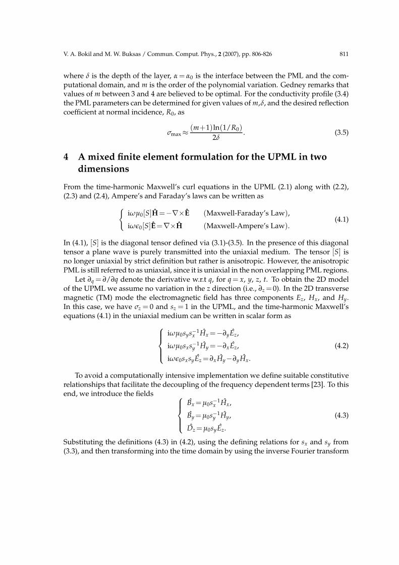
where δ is the depth of the layer, α = α0 is the interface between the PML and the com-putational domain, and m is the order of the polynomial variation. Gedney remarks thatvalues of m between 3 and 4 are believed to be optimal. For the conductivity profile (3.4)the PML parameters can be determined for given values of m,δ, and the desired reflectioncoefficient at normal incidence, R0, as

σmax≈(m+1)ln(1/R0)

2δ. (3.5)

4 A mixed finite element formulation for the UPML in two

dimensions

From the time-harmonic Maxwell’s curl equations in the UPML (2.1) along with (2.2),(2.3) and (2.4), Ampere’s and Faraday’s laws can be written as

iωµ0[S]H=−∇×E (Maxwell-Faraday’s Law),

iωǫ0[S]E=∇×H (Maxwell-Ampere’s Law).(4.1)

In (4.1), [S] is the diagonal tensor defined via (3.1)-(3.5). In the presence of this diagonaltensor a plane wave is purely transmitted into the uniaxial medium. The tensor [S] isno longer uniaxial by strict definition but rather is anisotropic. However, the anisotropicPML is still referred to as uniaxial, since it is uniaxial in the non overlapping PML regions.

Let ∂q = ∂/∂q denote the derivative w.r.t q, for q = x, y, z, t. To obtain the 2D modelof the UPML we assume no variation in the z direction (i.e., ∂z =0). In the 2D transversemagnetic (TM) mode the electromagnetic field has three components Ez, Hx, and Hy.In this case, we have σz = 0 and sz = 1 in the UPML, and the time-harmonic Maxwell’sequations (4.1) in the uniaxial medium can be written in scalar form as

iωµ0sys−1x Hx =−∂yEz,

iωµ0sxs−1y Hy =−∂xEz,

iωǫ0sxsyEz =∂xHy−∂yHx.

(4.2)

To avoid a computationally intensive implementation we define suitable constitutiverelationships that facilitate the decoupling of the frequency dependent terms [23]. To thisend, we introduce the fields

Bx =µ0s−1x Hx,

By =µ0s−1y Hy,

Dz =µ0syEz.

(4.3)

Substituting the definitions (4.3) in (4.2), using the defining relations for sx and sy from(3.3), and then transforming into the time domain by using the inverse Fourier transform


yields an equivalent system of time-domain differential equations given as

∂tB=− 1

ǫ0Σ2B−−→

curlE,

∂tH=1

µ0∂tB+

1

ǫ0µ0Σ1B,

∂tD=− 1

ǫ0σxD+curlH,

∂tE=− 1

ǫ0σyE+

1

ǫ0∂tD.

(4.4)

In the above H=(Hx,Hy)T, B=(Bx,By)T, E=Ez and D= Dz. Also, in (4.4)

Σ1 =

(

σx 00 σy

)

; Σ2 =

(

σy 00 σx

)

. (4.5)

Let D denote the computational domain in R2. We denote the domain D along with the

surrounding finite PML layers by Ω. In (4.4), the operators denoted by−→curl, and curl are

linear differential operators which are defined as

−→curlφ=(∂yφ,−∂xφ)T, ∀ φ∈D′(Ω), (4.6)

curlv=∂xvy−∂yvx, ∀ v=(vx,vy)T ∈D′(Ω)2, (4.7)

where D′(Ω) is the space of distributions on Ω. The operator curl appears as the (formal)

transpose of the operator−→curl [13], i.e.,

〈curlv,φ〉= 〈v,−→curlφ〉, ∀v∈D′(Ω)2, φ∈D′(Ω), (4.8)

with 〈·,·〉 being the appropriate inner product. Thus, the PML model consists in solvingsystem (4.4) for the six variables Bx, By, Hx, Hy, D, E in Ω, with PEC conditions on ∂Ω toterminate the PML; namely, n×E=0, on ∂Ω, where n is the outward unit normal to ∂Ω.In the case of the 2D TM mode the PEC condition translates to E=Ez =0, on ∂Ω.

Based on the above discussion, we consider the following variational formulation ofsystem (4.4) which is suitable for discretization by finite elements.

Find (E(·,t), D(·,t), H(·,t), B(·,t)) ∈ H10(Ω)×H1

0(Ω)×[L2(Ω)]2×[L2(Ω)]2 such thatfor all Ψ∈ [L2(Ω)]2, for all φ∈H1

0(Ω),

d

dt

∫

ΩB·Ψ dx=− 1

ǫ0

∫

ΩΣ2B·Ψ dx−

∫

Ω

−→curlE·Ψ dx,

d

dt

∫

ΩH·Ψ dx=

1

µ0

d

dt

∫

ΩB·Ψ dx+

1

ǫ0µ0

∫

ΩΣ1B·Ψ dx,

d

dt

∫

ΩD ·φ dx=− 1

ǫ0

∫

ΩσxD ·φ dx+

∫

Ω

−→curlφ·H dx,

d

dt

∫

ΩE·φ dx=− 1

ǫ0

∫

ΩσyE·φ dx+

1

ǫ0

d

dt

∫

ΩD ·φ dx,

(4.9)


K

E

E

E

E

Hy

Hy

Hx Hx

Edge 1

Edge 2

Edge

3

Edge

4

ex -

ey

?

6

6

6

- -

u u

u u

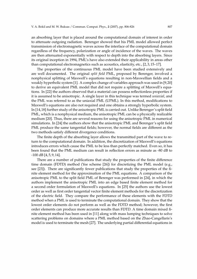
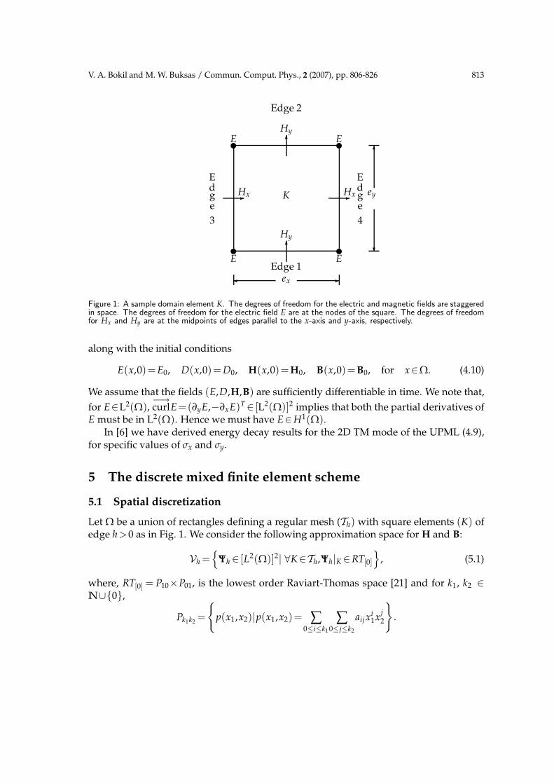
Figure 1: A sample domain element K. The degrees of freedom for the electric and magnetic fields are staggeredin space. The degrees of freedom for the electric field E are at the nodes of the square. The degrees of freedomfor Hx and Hy are at the midpoints of edges parallel to the x-axis and y-axis, respectively.

along with the initial conditions

E(x,0)=E0, D(x,0)= D0, H(x,0)=H0, B(x,0)=B0, for x∈Ω. (4.10)

We assume that the fields (E,D,H,B) are sufficiently differentiable in time. We note that,

for E∈L2(Ω),−→curlE=(∂yE,−∂xE)T∈ [L2(Ω)]2 implies that both the partial derivatives of

E must be in L2(Ω). Hence we must have E∈H1(Ω).In [6] we have derived energy decay results for the 2D TM mode of the UPML (4.9),

for specific values of σx and σy.

5 The discrete mixed finite element scheme

5.1 Spatial discretization

Let Ω be a union of rectangles defining a regular mesh (Th) with square elements (K) ofedge h>0 as in Fig. 1. We consider the following approximation space for H and B:

Vh =

Ψh ∈ [L2(Ω)]2| ∀K∈Th,Ψh|K ∈RT[0]

, (5.1)

where, RT[0] = P10×P01, is the lowest order Raviart-Thomas space [21] and for k1, k2 ∈N∪0,

Pk1k2=

p(x1,x2)|p(x1,x2)= ∑0≤i≤k1

∑0≤j≤k2

aijxi1x

j2

.


The basis functions for Hx have unity value along an ey edge and are zero over all otheredges. Similarly, the basis functions for Hy have unity value along an ex edge and arezero over all other edges (see Fig. 1).

The approximation space for E and D is chosen to be

Uh =φh ∈H10(Ω)| ∀K∈Th,φh|K ∈Q1, (5.2)

where the space Q1 = P11. The basis functions for E have unity value at one node andare zero at all other nodes. Fig. 1 shows the locations for the degrees of freedom for theelectric and magnetic fields.

Based on the approximation spaces described above the spatially discrete scheme is:Find (Eh(·,t),Dh(·,t),Hh(·,t),Bh(·,t))∈Uh×Uh×Vh×Vh such that for all Ψh ∈Vh, and forall φh∈Uh,

d

dt

∫

ΩBh ·Ψhdx=− 1

ǫ0

∫

ΩΣ1Bh ·Ψhdx−

∫

Ω

−→curlEh ·Ψhdx,

d

dt

∫

ΩHh ·Ψhdx=

1

µ0

d

dt

∫

ΩBh ·Ψhdx+

1

ǫ0µ0

∫

ΩΣ2Bh ·Ψhdx,

d

dt

∫

ΩDh ·φh dx=− 1

ǫ0

∫

ΩσxDh ·φh dx+

∫

Ω

−→curlφh ·Hh dx,

d

dt

∫

ΩEh ·φh dx=− 1

ǫ0

∫

ΩσyEh ·φh dx+

1

ǫ0

d

dt

∫

ΩDh ·φh dx.

(5.3)

5.2 Temporal discretization

For the temporal discretization we use a centered second order accurate finite differencescheme. For k∈Z let,

D∆tVk =

Vk+1/2−Vk−1/2

∆t, V

k=

Vk+1/2+Vk−1/2

2. (5.4)

Let (·,·) denote the inner product in L2(Ω). We can now describe the fully discrete

scheme in space and time as: Find (En+1h ,Dn+1

h ,Hn+ 1

2

h ,Bn+ 1

2

h )∈Uh×Uh×Vh×Vh such thatfor all Ψh ∈Vh, for all φh∈Uh,

(i) (D∆tBnh ,Ψh)=− 1

ǫ0(Σ2Bn

h ,Ψh)−(−→curlEn

h , Ψh),

(ii) (D∆tHnh ,Ψh)=

1

µ0(D∆tB

nh ,Ψh)+

1

ǫ0µ0(Σ1Bn

h ,Ψh),

(iii) (D∆tDn+ 1

2

h ,φh)=− 1

ǫ0(σxDh

n+ 12 ,φh)+(

−→curlφh,H

n+ 12

h ),

(iv) (D∆tEn+ 1

2

h ,φh)=− 1

ǫ0(σyEh

n+ 12 ,φh)+

1

ǫ0(D∆tD

n+ 12

h , φh).

(5.5)


6 Analysis of the discrete PML model

In this section we study the properties of the discrete mixed FEM-UPML model by per-forming a plane wave analysis to calculate the reflection coefficient. We refer the readerto [6] for a detailed stability and dispersion analysis of the mixed FEM method for thediscretization of the UPML and a comparison with the FDTD scheme.

In the discrete setting the PML model is no longer perfectly matched since the dis-cretization introduces some error which manifests itself as spurious reflections. There isalso error that is introduced due to the termination of the PML. We study the errors in-troduced in the discrete model by calculating the reflection coefficient of an infinite PML(to study the errors caused by the discretization) as well as the reflection coefficient of afinite PML (to study the errors introduced by terminating the PML).

For simplicity we assume in this section that ǫ0=µ0=1. Let us also assume an infinitePML in the region x>0. Thus, σy =0 and let σx =σ. Considering exact integration in time,we will look for solutions of the form

V(x,y,t)= V(x,y)eiωt, (6.1)

to the semi-discrete system (5.3). Substituting (6.1) in (5.3), we obtain the time harmonicsystem

iω(Bx,ψx)=−(

∂yE,ψx

)

,

iω(Hx,ψx)= iω((

1+σ

iω

)

Bx,ψx

)

,

iω((

1+σ

iω

)

By,ψy

)

=(

∂xE,ψy

)

,

iω(Hy,ψy)= iω(By,ψy),

iω((

1+σ

iω

)

D,φ)

=(

Hx,∂yφ)

−(

Hy,∂xφ)

,

iω(E,φ)= iω(D,φ).

(6.2)

We assume that σ is a piecewise constant function of x with jumps at x = lh,l = 0,1,2,.. .,where h=hx =hy is the mesh step size. Let

σl =

Value of σ on (lh,(l+1)h), if l≥0,

0, if l <0.(6.3)

Using the definition (3.3), we have

sx,l = sl =1+σl

iω. (6.4)

Since σy = 0, we have sy = 1. The PML is in the half space x > 0 and the computationaldomain is in the half space x < 0. Therefore, x = 0 is the interface between the PML and


d

d

d

d d d

d

d

d

d

El−1,m−1

El−1,m

El−1,m+1

El,m−1

El,m+1

El,m

El+1,m−1

El+1,m

El+1,m+1

6 6

6 6

6 6

-

-

-

-

-

-

Hl−1,m−1/2

Hl−1,m+1/2

Hl,m−1/2

Hl,m+1/2

Hl+1,m−1/2

Hl+1,m+1/2

Hl−1/2,m−1 Hl+1/2,m−1

Hl−1/2,m Hl+1/2,m

Hl−1/2,m+1 Hl+1/2,m+1

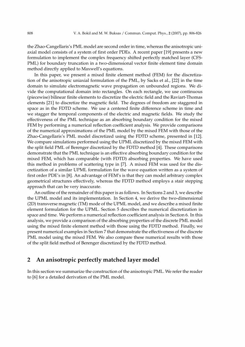
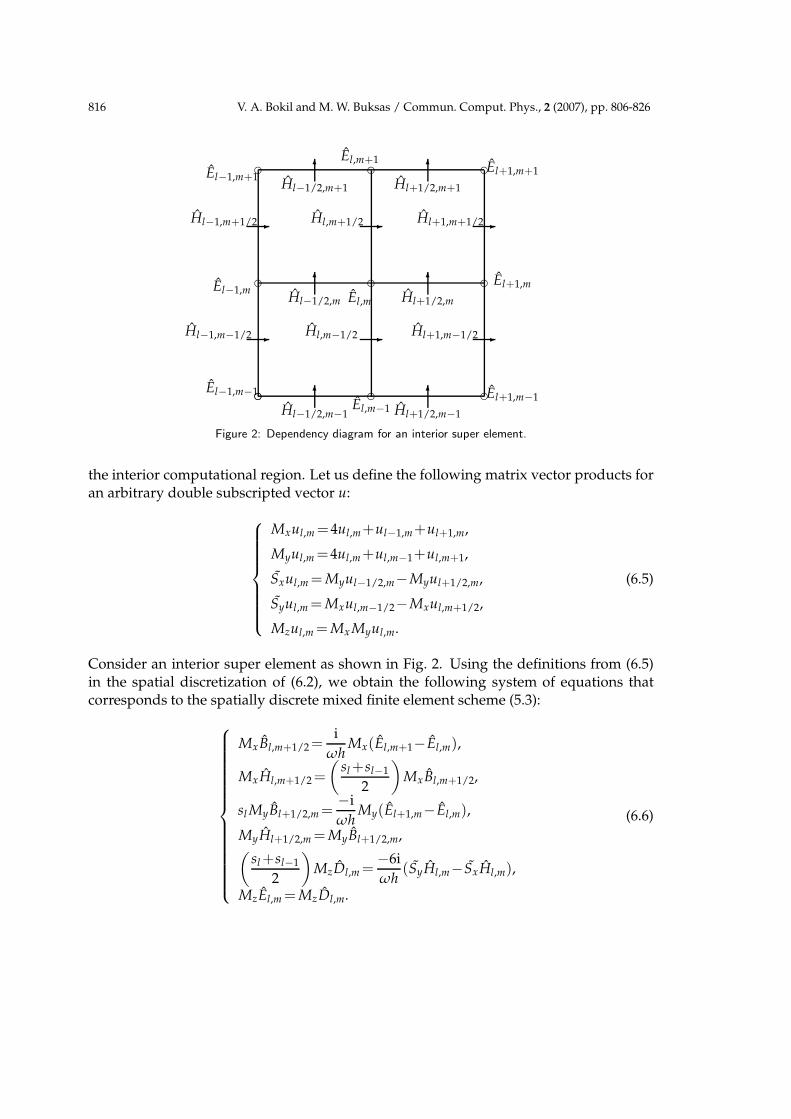
Figure 2: Dependency diagram for an interior super element.

the interior computational region. Let us define the following matrix vector products foran arbitrary double subscripted vector u:

Mxul,m =4ul,m+ul−1,m+ul+1,m,

Myul,m =4ul,m+ul,m−1+ul,m+1,

Sxul,m = Myul−1/2,m−Myul+1/2,m,

Syul,m = Mxul,m−1/2−Mxul,m+1/2,

Mzul,m = Mx Myul,m.

(6.5)

Consider an interior super element as shown in Fig. 2. Using the definitions from (6.5)in the spatial discretization of (6.2), we obtain the following system of equations thatcorresponds to the spatially discrete mixed finite element scheme (5.3):

Mx Bl,m+1/2 =i

ωhMx(El,m+1−El,m),

MxHl,m+1/2 =

(

sl +sl−1

2

)

Mx Bl,m+1/2,

sl MyBl+1/2,m =−i

ωhMy(El+1,m−El,m),

MyHl+1/2,m = MyBl+1/2,m,(

sl +sl−1

2

)

MzDl,m =−6i

ωh(SyHl,m−SxHl,m),

MzEl,m = MzDl,m.

(6.6)


Combining the equations in (6.6), we obtain an equation in E by eliminating the othervariables

−ω2h2

6

(

sl +sl−1

2

)

MzEl,m =

(

sl +sl−1

2

)

(MxEl,m+1−2MxEl,m+MxEl,m−1)

+1

sl(MyEl+1,m−MyEl,m)− 1

sl−1(MyEl,m−MyEl−1,m). (6.7)

We now look for solutions to (6.7) of the form

El,m = Ele−ikymh. (6.8)

After substituting (6.8) in (6.7), and performing some algebra, we obtain

− ζω2h2

6

(

sl +sl−1

2

)

(4El +El−1+El+1)=1

sl(El+1−El)−

1

sl−1(El−El−1), (6.9)

where the coefficient ζ is defined as

ζ =1− 12

ω2h2

(

sin2(kyh/2)

1+2cos2(kyh/2)

)

. (6.10)

Let kx and kpmlx be the x components of the wave vector in free space and the PML, respec-

tively. To calculate the reflection coefficient for the infinite PML, we look for solutions to(6.9) of the form

El =

e−ikxhl +Reikxhl , for l <0,

Te−kpmlx hl, for l >0,

(6.11)

where the reflection coefficient is R, and T is the transmission coefficient. Consider theequations associated to the node at the interface l =0 and one node each on either side ofthe interface at l =1, and l =−1. From (6.9) we have

− ζω2h2

6(4E−1+E−2+E0)=(E0−E−1)−(E−1−E−2),

− ζω2h2

6

(

1+s0

2

)

(4E0+E−1+E1)=1

s0(E1−E0)−(E0−E−1),

− ζω2h2

6

(

s1+s0

2

)

(4E1+E0+E2)=1

s1(E2−E1)−

1

s0(E1−E0),

(6.12)

where ζ is defined in (6.10), and sl is defined in (6.4). Substituting for El from (6.11) in(6.12) we obtain three equations in the unknowns E0, R and T. Solving these resultingequations for R, we can show that the reflection coefficient has the Taylor series expansion

R=− 1

16ω2(ω2−k2

y)σ(σ+2iω)h2 +1

48ω3σ2(σ+2iω)(ω2−k2

y)3/2h3+O(h4). (6.13)


The formula (6.13) implies that the reflection coefficient is proportional to h2.Next, we study the effects of terminating the PML by a PEC. This amounts to setting

E=0 at the boundary x=δ=Nh of the PML, i.e. EN=0. Here, N is the number of nodes perwavelength, i.e., the thickness of the PML is one wavelength and the number of nodesper wavelength is equal to the number of nodes in the PML. To obtain the reflectioncoefficient we write equation (6.9) for all the nodes in the PML as well as for the node atthe interface of the working volume and PML, E0, and node E−1 in the working volumewhich is h distance away from the interface. Assuming that we know the value of E−2

we obtain a system of equations

AE=−(ω2h2ζ+6)E−2 e1. (6.14)

In the above E=[E−1,E0,E1,··· ,EN−1]T, e1 =[1,0,0,··· ]T and the matrix of coefficients ob-

tained from (6.9) is

A=

b−1 c0 0 ... 0a−1 b0 c1 0 ... 0

0 a0 b1 c2. . .

......

. . .. . .

. . .. . . 0

cN−1

0 0 ... 0 aN−2 bN−1

, (6.15)

where

al = ζω2h2

(

sl+1+sl

2

)

+6

sl,

bl =4ζω2h2

(

sl−1+sl

2

)

−6

(

1

sl+

1

sl−1

)

,

cl = ζω2h2

(

sl−1+sl−2

2

)

+6

sl−1.

(6.16)

We can solve system (6.15) for the value of R by using (6.11) for l =−1 and l =−2. In thiscase the reflection coefficient is calculated to be

R=−e2ikxh

(

1+(ω2h2ζ+6)κ eikxh

1+(ω2h2ζ+6)κe−ikx h

)

, (6.17)

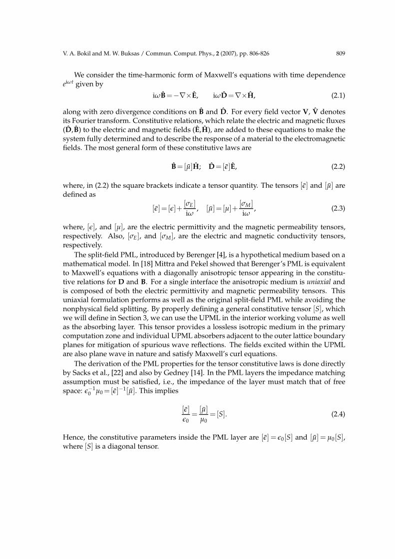
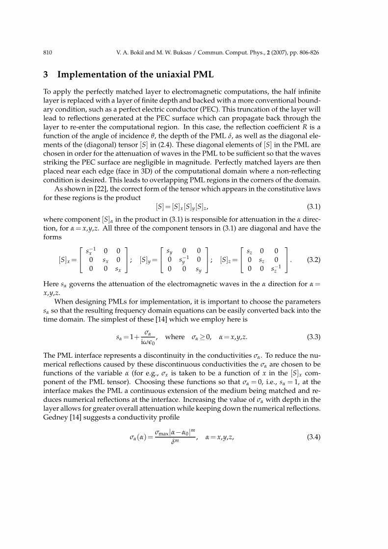
where κ is the first diagonal entry in A−1.Fig. 3 plots the reflection coefficient in decibels, Db (i.e., 20log10 R), versus the number

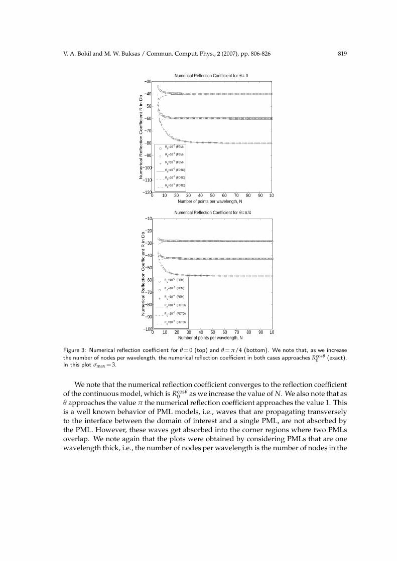
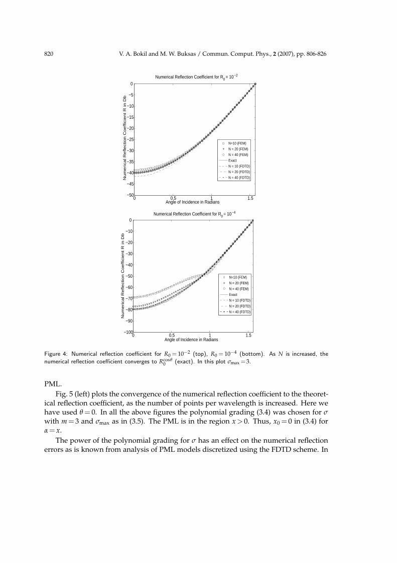
of nodes per wavelength N for different values of R0, the reflection coefficient at normalincidence for θ =0 (top) and θ =π/4 (bottom). Fig. 4 plots the reflection coefficient in Dbversus the angle of incidence θ for R0=10−2 (top) and R0=10−4 (bottom). In these figureswe compare the reflection coefficient for the mixed FEM scheme with the reflection co-efficient for the TE mode of the Zhao-Cangellaris’s PML model using the FDTD schemewhich was presented in [12]. As can be seen in these plots the reflection properties of theFEM compare well with those of the FDTD method.


0 10 20 30 40 50 60 70 80 90 100−120

−110

−100

−90

−80

−70

−60

−50

−40

−30

Number of points per wavelength, N

Nu

me

rica

l R

efle

ctio

n C

oe

ffic

ien

t R

in

Db

Numerical Reflection Coefficient for θ = 0

R0=10−2 (FEM)

R0=10−3 (FEM)

R0=10−4 (FEM)

R0=10−2 (FDTD)

R0=10−3 (FDTD)

R0=10−4 (FDTD)

0 10 20 30 40 50 60 70 80 90 100−100

−90

−80

−70

−60

−50

−40

−30

−20

−10

Number of points per wavelength, N

Nu

me

rica

l R

efle

ctio

n C

oe

ffic

ien

t R

in

Db

Numerical Reflection Coefficient for θ = π/4

R0=10−2 (FEM)

R0=10−3 (FEM)

R0=10−4 (FEM)

R0=10−2 (FDTD)

R0=10−3 (FDTD)

R0=10−4 (FDTD)

Figure 3: Numerical reflection coefficient for θ =0 (top) and θ = π/4 (bottom). We note that, as we increase

the number of nodes per wavelength, the numerical reflection coefficient in both cases approaches Rcosθ0 (exact).

In this plot σmax =3.

We note that the numerical reflection coefficient converges to the reflection coefficientof the continuous model, which is Rcosθ

0 as we increase the value of N. We also note that asθ approaches the value π the numerical reflection coefficient approaches the value 1. Thisis a well known behavior of PML models, i.e., waves that are propagating transverselyto the interface between the domain of interest and a single PML, are not absorbed bythe PML. However, these waves get absorbed into the corner regions where two PMLsoverlap. We note again that the plots were obtained by considering PMLs that are onewavelength thick, i.e., the number of nodes per wavelength is the number of nodes in the


0 0.5 1 1.5−50

−45

−40

−35

−30

−25

−20

−15

−10

−5

0

Angle of Incidence in Radians

Nu

me

rica

l R

efle

ctio

n C

oe

ffic

ien

t R

in

Db

Numerical Reflection Coefficient for R0 = 10−2

N=10 (FEM)

N = 20 (FEM)

N = 40 (FEM)

Exact

N = 10 (FDTD)

N = 20 (FDTD)

N = 40 (FDTD)

0 0.5 1 1.5−100

−90

−80

−70

−60

−50

−40

−30

−20

−10

0

Angle of Incidence in Radians

Nu

me

rica

l R

efle

ctio

n C

oe

ffic

ien

t R

in

Db

Numerical Reflection Coefficient for R0 = 10−4

N=10 (FEM)

N = 20 (FEM)

N = 40 (FEM)

Exact

N = 10 (FDTD)

N = 20 (FDTD)

N = 40 (FDTD)

Figure 4: Numerical reflection coefficient for R0 = 10−2 (top), R0 = 10−4 (bottom). As N is increased, the

numerical reflection coefficient converges to Rcosθ0 (exact). In this plot σmax =3.

PML.

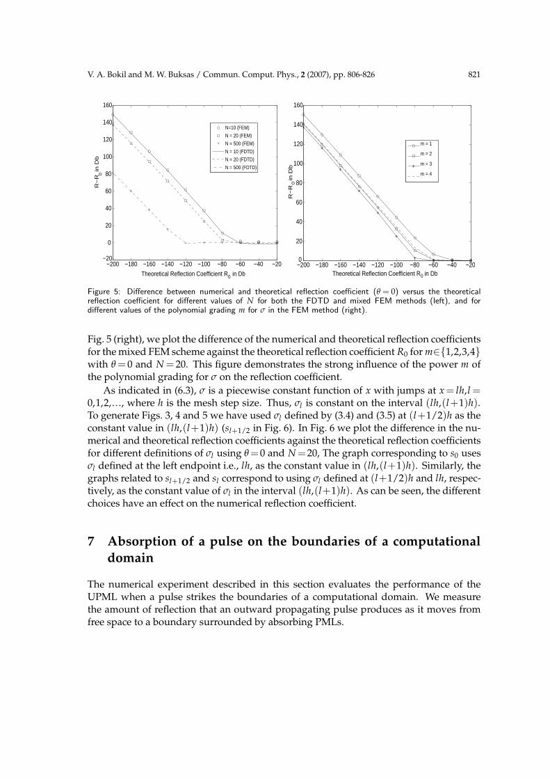
Fig. 5 (left) plots the convergence of the numerical reflection coefficient to the theoret-ical reflection coefficient, as the number of points per wavelength is increased. Here wehave used θ = 0. In all the above figures the polynomial grading (3.4) was chosen for σwith m = 3 and σmax as in (3.5). The PML is in the region x > 0. Thus, x0 = 0 in (3.4) forα= x.

The power of the polynomial grading for σ has an effect on the numerical reflectionerrors as is known from analysis of PML models discretized using the FDTD scheme. In


−200 −180 −160 −140 −120 −100 −80 −60 −40 −20−20

0

20

40

60

80

100

120

140

160

Theoretical Reflection Coefficient R0 in Db

R−

R0 i

n D

b

N=10 (FEM)

N = 20 (FEM)

N = 500 (FEM)

N = 10 (FDTD)

N = 20 (FDTD)

N = 500 (FDTD)

−200 −180 −160 −140 −120 −100 −80 −60 −40 −200

20

40

60

80

100

120

140

160


R−

R0

in D

b

m = 1

m = 2

m = 3

m = 4

Figure 5: Difference between numerical and theoretical reflection coefficient (θ = 0) versus the theoreticalreflection coefficient for different values of N for both the FDTD and mixed FEM methods (left), and fordifferent values of the polynomial grading m for σ in the FEM method (right).

Fig. 5 (right), we plot the difference of the numerical and theoretical reflection coefficientsfor the mixed FEM scheme against the theoretical reflection coefficient R0 for m∈1,2,3,4with θ = 0 and N = 20. This figure demonstrates the strong influence of the power m ofthe polynomial grading for σ on the reflection coefficient.

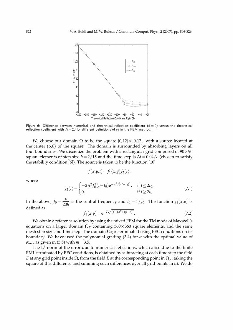
As indicated in (6.3), σ is a piecewise constant function of x with jumps at x = lh,l =0,1,2,.. ., where h is the mesh step size. Thus, σl is constant on the interval (lh,(l+1)h).To generate Figs. 3, 4 and 5 we have used σl defined by (3.4) and (3.5) at (l+1/2)h as theconstant value in (lh,(l+1)h) (sl+1/2 in Fig. 6). In Fig. 6 we plot the difference in the nu-merical and theoretical reflection coefficients against the theoretical reflection coefficientsfor different definitions of σl using θ =0 and N =20, The graph corresponding to s0 usesσl defined at the left endpoint i.e., lh, as the constant value in (lh,(l+1)h). Similarly, thegraphs related to sl+1/2 and sl correspond to using σl defined at (l+1/2)h and lh, respec-tively, as the constant value of σl in the interval (lh,(l+1)h). As can be seen, the differentchoices have an effect on the numerical reflection coefficient.

7 Absorption of a pulse on the boundaries of a computational

domain

The numerical experiment described in this section evaluates the performance of theUPML when a pulse strikes the boundaries of a computational domain. We measurethe amount of reflection that an outward propagating pulse produces as it moves fromfree space to a boundary surrounded by absorbing PMLs.


−200 −180 −160 −140 −120 −100 −80 −60 −40 −20−20

0

20

40

60

80

100

120

140


R−

R0

in D

b

sl,0

sl,1/2

sl,1

Figure 6: Difference between numerical and theoretical reflection coefficient (θ = 0) versus the theoreticalreflection coefficient with N =20 for different definitions of σl in the FEM method.

We choose our domain Ω to be the square [0,12]×[0,12], with a source located atthe center (6,6) of the square. The domain is surrounded by absorbing layers on allfour boundaries. We discretize the problem with a rectangular grid composed of 90×90square elements of step size h = 2/15 and the time step is ∆t = 0.04/c (chosen to satisfythe stability condition [6]). The source is taken to be the function [10]

f (x,y,t)= f1(x,y) f2(t),

where

f2(t)=

−2π2 f 20 (t−t0)e−π2 f 2

0 (t−t0)2, if t≤2t0,

0, if t≥2t0.(7.1)

In the above, f0 =c

20his the central frequency and t0 = 1/ f0. The function f1(x,y) is

defined asf1(x,y)=e−7

√(x−6)2+(y−6)2

. (7.2)

We obtain a reference solution by using the mixed FEM for the TM mode of Maxwell’sequations on a larger domain ΩR containing 360×360 square elements, and the samemesh step size and time step. The domain ΩR is terminated using PEC conditions on itsboundary. We have used the polynomial grading (3.4) for σ with the optimal value ofσmax as given in (3.5) with m=3.5.

The L2 norm of the error due to numerical reflections, which arise due to the finitePML terminated by PEC conditions, is obtained by subtracting at each time step the fieldE at any grid point inside Ω, from the field E at the corresponding point in ΩR, taking thesquare of this difference and summing such differences over all grid points in Ω. We do


0 100 200 300 400 500 60010

−16

10−14

10−12

10−10

10−8

10−6

10−4

10−2

Reference Error FEMSF

4 cell PML

8 cell PML

16 cell PML

Time Step

L2

erro

ro

nth

e90

×90

cell

sg

rid

0 100 200 300 400 500 60010

−16

10−14

10−12

10−10

10−8

10−6

10−4

10−2 Reference Error

FEMSF

4 cell PML

8 cell PML

16 cell PML

Time Step

L2

erro

ro

nth

e18

0×

180

cell

sg

rid

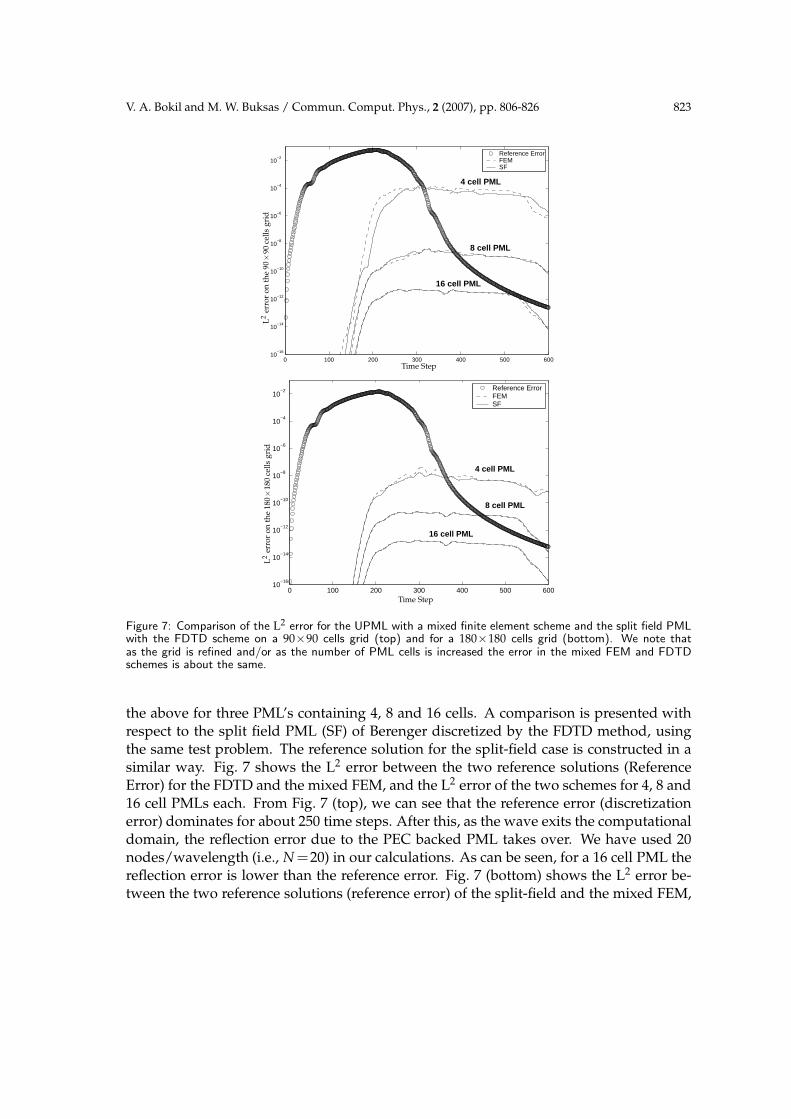
Figure 7: Comparison of the L2 error for the UPML with a mixed finite element scheme and the split field PMLwith the FDTD scheme on a 90×90 cells grid (top) and for a 180×180 cells grid (bottom). We note thatas the grid is refined and/or as the number of PML cells is increased the error in the mixed FEM and FDTDschemes is about the same.

the above for three PML’s containing 4, 8 and 16 cells. A comparison is presented withrespect to the split field PML (SF) of Berenger discretized by the FDTD method, usingthe same test problem. The reference solution for the split-field case is constructed in asimilar way. Fig. 7 shows the L2 error between the two reference solutions (ReferenceError) for the FDTD and the mixed FEM, and the L2 error of the two schemes for 4, 8 and16 cell PMLs each. From Fig. 7 (top), we can see that the reference error (discretizationerror) dominates for about 250 time steps. After this, as the wave exits the computationaldomain, the reflection error due to the PEC backed PML takes over. We have used 20nodes/wavelength (i.e., N =20) in our calculations. As can be seen, for a 16 cell PML thereflection error is lower than the reference error. Fig. 7 (bottom) shows the L2 error be-tween the two reference solutions (reference error) of the split-field and the mixed FEM,


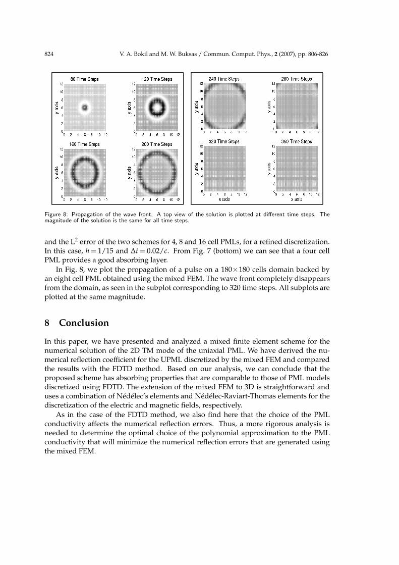
Figure 8: Propagation of the wave front. A top view of the solution is plotted at different time steps. Themagnitude of the solution is the same for all time steps.

and the L2 error of the two schemes for 4, 8 and 16 cell PMLs, for a refined discretization.In this case, h = 1/15 and ∆t = 0.02/c. From Fig. 7 (bottom) we can see that a four cellPML provides a good absorbing layer.

In Fig. 8, we plot the propagation of a pulse on a 180×180 cells domain backed byan eight cell PML obtained using the mixed FEM. The wave front completely disappearsfrom the domain, as seen in the subplot corresponding to 320 time steps. All subplots areplotted at the same magnitude.

8 Conclusion

In this paper, we have presented and analyzed a mixed finite element scheme for thenumerical solution of the 2D TM mode of the uniaxial PML. We have derived the nu-merical reflection coefficient for the UPML discretized by the mixed FEM and comparedthe results with the FDTD method. Based on our analysis, we can conclude that theproposed scheme has absorbing properties that are comparable to those of PML modelsdiscretized using FDTD. The extension of the mixed FEM to 3D is straightforward anduses a combination of Nedelec’s elements and Nedelec-Raviart-Thomas elements for thediscretization of the electric and magnetic fields, respectively.

As in the case of the FDTD method, we also find here that the choice of the PMLconductivity affects the numerical reflection errors. Thus, a more rigorous analysis isneeded to determine the optimal choice of the polynomial approximation to the PMLconductivity that will minimize the numerical reflection errors that are generated usingthe mixed FEM.


Acknowledgments

The authors would like to thank Dr. H. T. Banks, Dr. R. Glowinski, and Dr. Mac Hymanfor fruitful discussions and for their tremendous support and encouragement. This workwas supported in part by Los Alamos National Laboratory, an affirmative action/equalopportunity employer which is operated by the University of California for the UnitedStates Department of Energy under contract Nos W-7405-ENG-36, 03891-001-99-4G, 74837-001-03 49, and/or 86192-001-04 49, and in part by the U.S. Air Force Office of ScientificResearch under grants AFOSR F49620-01-1-0026 and AFOSR FA9550-04-1-0220.

References

[1] S. Abarbanel and D. Gottlieb, A mathematical analysis of the PML method, J. Comput. Phys.,134 (1997), 357-363.

[2] S. Abarbanel, D. Gottlieb and J. S. Hesthaven, Well-posed perfectly matched layers for ad-vective acoustics, J. Comput. Phys., 154 (1999), 266-283.

[3] A. Ahland, D. Schulz and E. Voges, Accurate mesh truncation for Schrodinger equations bya perfectly matched layer absorber: Application to the calculation of optical spectra, Phys.Rev. B, 60 (1999), 109-112.

[4] J. P. Berenger, A perfectly matched layer for the absorption of electromagnetic waves, J.Comput. Phys., 114 (1994), 185-200.

[5] J. P. Berenger, Three dimensional perfectly matched layer for the absorption of electromag-netic waves, J. Comput. Phys., 127 (1996), 363-379.

[6] V. A. Bokil and M. W. Buksas, Comparison of a finite difference and a mixed finite elementformulation of the uniaxial perfectly matched layer, Tech. Rep. CRSC-TR06-12, N. C. StateUniversity, February 2006.

[7] V. A. Bokil and R. Glowinski, A distributed Lagrange multiplier based fictitious domainmethod for Maxwell’s equations, Int. J. Comput. Numer. Anal. Appl., 6 (2004), 203-245.

[8] V. A. Bokil and R. Glowinski, An operator splitting scheme with a distributed Lagrange mul-tiplier based fictitious domain method for wave propagation problems, J. Comput. Phys.,205 (2005), 242-268.

[9] W. C. Chew and W. H. Weedon, A 3D perfectly matched medium from modified Maxwellsequations with stretched coordinates, Microw. Opt. Techn. Lett., 7 (1994), 599-604.

[10] G. Cohen, P. Joly, J. Roberts and N. Tordjman, Higher order triangular finite elements withmass lumping for the wave equation, SIAM J. Numer. Anal., 38 (2001), 2047-2078.

[11] G. Cohen and P. Monk, Mur-Nedelec finite element schemes for Maxwell’s equations, Com-put. Method. Appl. Mech. Engrg., 169 (1999), 197-217.

[12] F. Collino and P. Monk, Optimizing the perfectly matched layer, Comput. Method. Appl.Mech. Engrg., 164 (1998), 157-171.

[13] R. Dautray and J.-L. Lions, Mathematical Analysis and Numerical Methods for Science andTechnology, vol. 3, Springer-Verlag, Berlin Heidelberg, 1990.

[14] S. D. Gedney, An anisotropic perfectly matched layer absorbing media for the truncation ofFDTD lattices, IEEE T. Antenn. Propag., 44 (1996), 1630-1639.

[15] M. E. Hayder, F. Q. Hu and M. Y. Hussaini, Towards perfectly absorbing conditions for Eulerequations, in: AIAA 13th CFD Conference, Paper 97-2075, 1997.


[16] F. Q. Hu, On absorbing boundary conditions for linearized Euler equations by a perfectlymatched layer, J. Comput. Phys., 129 (1996), 201-219.

[17] D. Johnson, C. Furse and A. Tripp, Application and optimization of the perfectly matchedlayer boundary condition for geophysical simulations, Microw. Opt. Techn. Lett., 25 (2000),254-255.

[18] R. Mittra and U. Pekel, A new look at the perfectly matched layer (PML) concept for the re-flectionless absorption of electromagnetic waves, IEEE Microw. Guided Wave Lett., 5 (1995),84-86.

[19] M. Movahhedi, A. Abdipour, H. Ceric, A. Sheikholeslami and S. Selberherr, Optimization ofthe perfectly matched layer for the finite-element time-domain method, IEEE Microw. Wirel.Components Lett., 17(1) (2007), 10-12.

[20] C. M. Rappaport, Perfectly matched absorbing boundary conditions based on anisotropiclossy mapping of space, IEEE Microw. Guided Wave Lett., 5 (1995), 90-92.

[21] P. A. Raviart and J. M. Thomas, A mixed finite element method for 2nd order elliptic prob-lems, in: I. Galligani and E. Magenes (Eds.), Proc. of Math. Aspects on the Finite ElementMethod, Lecture Notes in Mathematics, Springer-Verlag, vol. 606, 1977, pp. 292-315.

[22] Z. S. Sacks, D. M. Kinsland, R. Lee and J. F. Lee, A perfectly matched anisotropic absorberfor use as an absorbing boundary condition, IEEE T. Antenn. Propag., 43 (1995), 1460-1463.

[23] A. Taflove, Advances in Computational Electrodynamics: The Finite-Difference Time-Domain Method, Artech House, Norwood, MA, 1998.

[24] J. We, D. Kinsland, J. Lee and R. Lee, A comparison of anistropic PML to Berenger’s PMLand it’s application to the finite-element method of EM scattering, IEEE T. Antenn. Propag.,45 (1997), 40-50.

[25] J.-Y. Wu, J. Nehrbass and R. Lee, A comparison of PML for TVFEM and FDTD, Int. J. Numer.Model., 13 (2000), 233-244.

[26] K. S. Yee, Numerical solution of initial boundary value problems involving Maxwell’s equa-tions in isotropic media, IEEE T. Antenn. Propag., 14 (1966), 302-307.

[27] L. Zhao and A. Cangellaris, A general approach for the development of unsplit-field time-domain implementations of perfectly matched layers for FDTD grid truncation, IEEE Mi-crow. Guided Wave Lett., 6 (1996), 209-211.

Date post:	23-Feb-2022
Category:	Documents
Upload:	others
View:	16 times
Download:	0 times

Comparison of Finite Difference and Mixed Finite ...

Documents