Comparison of finite difference based methods to obtain sensitivities of stochastic chemical kinetic models Rishi Srivastava, David F. Anderson, and James B. Rawlings Citation: J. Chem. Phys. 138, 074110 (2013); doi: 10.1063/1.4790650 View online: http://dx.doi.org/10.1063/1.4790650 View Table of Contents: http://jcp.aip.org/resource/1/JCPSA6/v138/i7 Published by the American Institute of Physics. Additional information on J. Chem. Phys. Journal Homepage: http://jcp.aip.org/ Journal Information: http://jcp.aip.org/about/about_the_journal Top downloads: http://jcp.aip.org/features/most_downloaded Information for Authors: http://jcp.aip.org/authors
Transcript
Comparison of finite difference based methods to obtain sensitivities ofstochastic chemical kinetic modelsRishi Srivastava, David F. Anderson, and James B. Rawlings Citation: J. Chem. Phys. 138, 074110 (2013); doi: 10.1063/1.4790650 View online: http://dx.doi.org/10.1063/1.4790650 View Table of Contents: http://jcp.aip.org/resource/1/JCPSA6/v138/i7 Published by the American Institute of Physics. Additional information on J. Chem. Phys.Journal Homepage: http://jcp.aip.org/ Journal Information: http://jcp.aip.org/about/about_the_journal Top downloads: http://jcp.aip.org/features/most_downloaded Information for Authors: http://jcp.aip.org/authors
THE JOURNAL OF CHEMICAL PHYSICS 138, 074110 (2013)
Comparison of finite difference based methods to obtain sensitivitiesof stochastic chemical kinetic models
Rishi Srivastava,1,a) David F. Anderson,2,b) and James B. Rawlings1,c)
1Department of Chemical and Biological Engineering, University of Wisconsin-Madison,Madison, Wisconsin 53706, USA2 Department of Mathematics, University of Wisconsin-Madison, Madison, Wisconsin 53706, USA
(Received 24 September 2012; accepted 21 January 2013; published online 20 February 2013)
Recent years have seen an increasing popularity ofstochastic chemical kinetic models due to their role in de-scribing and explaining critical biological phenomena.3–9 Oneuseful tool for understanding these models is the chemicalmaster equation, which describes the evolution of the prob-ability density of the system. The solution of the masterequation is computationally tractable only for simple sys-tems. Rather, approximation techniques such as finite stateprojection,10 that operates on a reduced state space, or thestochastic simulation algorithm (SSA),11, 12 that generates ex-act sample paths, are employed to reconstruct a system’sprobability distribution and statistics (usually the mean andvariance). Applying these techniques to solve models of bi-ological processes leads to significant improvements in ourunderstanding of intrinsic noise and its effect on cellularbehavior.
These stochastic chemical kinetic models depend on pa-rameters whose values are often unknown and can change dueto changes in the environment. Sensitivities quantify the de-pendence of the system’s output to changes in the model pa-rameters. Sensitivity analysis is useful in determining param-eters to which the system output is most responsive, in as-sessing robustness of the system to extreme circumstances orunusual environmental conditions, and in identifying rate lim-iting pathways as a candidate for drug delivery. However, one
of the most important applications of sensitivities is in param-eter estimation. Sensitivities provide a way to approximate theHessian of the objective function through the Gauss-Newtonapproximation (Ref. 13, p. 535).
A popular unbiased method of sensitivity estimation isthe likelihood ratio gradient method.14–16 The unbiasednessof the likelihood ratio gradient method comes at the cost ofa high variance of the estimator if there are several reactionevents in the estimation of the output of interest. The conver-gence rate, which is a measure of the rate at which the meansquared error of the estimator converges to zero, of this es-timator is O(N−1/2), in which N is the number of estimatorsimulations. Komorowski et al.17 use a linear noise approx-imation of stochastic chemical kinetic models for sensitivityanalysis. However, use of linear noise approximation limitstheir analysis to only stochastic differential equation modelsthat incorporate Brownian motions. Gunawan et al.18 com-pare the sensitivity of the mean with the sensitivity of the en-tire distribution. They explain why the sensitivity of the meancan be inadequate in determining the sensitivity of stochasticchemical kinetic models.
Despite being easier to implement and intuitive to un-derstand, finite difference based methods produce biased sen-sitivity estimates. However, implemented with considerationof the trade-off between the statistical error of the estimatorand its bias, finite difference based methods can have a con-vergence rate close to the best possible convergence rate ofO(N−1/2).19 McGill et al.20 compare the applicability of likeli-hood ratio gradient and finite difference based methods. Theydiscuss situations where one method performs better than the
074110-2 Srivastava, Anderson, and Rawlings J. Chem. Phys. 138, 074110 (2013)
other. Drew et al.21 demonstrate usefulness of sensitivity anal-ysis on Monte Carlo simulations of copper electrodeposition.
Several different estimators using finite difference havebeen proposed.1, 2, 19 Anderson1 proposed a new estimator,coupled finite difference (CFD), using a single Markov chainfor the nominal and perturbed processes. The CFD estimatorincorporates a tight coupling between the nominal and per-turbed processes, thereby producing a significant reduction inestimator variance.1
In this paper, we show the superiority of CFD over CRNin the estimation of sensitivities. We do not discuss the inde-pendent random number2 estimator, also known as the CrudeMonte Carlo1 estimator, because either estimator, CRN orCFD, usually has several orders of magnitude smaller vari-ance than this estimator. We calculate sensitivity estimates offive different quantities of interest. In example one, the quan-tity of interest is the expected value of a species. Example twolooks at the likelihood of experimental data. Example threelooks at the probability of a rare state. Example four looks atthe expected value of a fast fluctuating species. Example fivelooks at the expected value of a gene product in a model ofa genetic toggle switch. In this example, the CRN method isshown to be superior to the CRP method, something not pre-viously observed in the literature.
This paper is arranged as follows. Section II definesthe estimators that are used in the subsequent examples.Section III shows the results we obtain from the five exam-ples. Finally, Sec. IV discusses the conclusions of this paperand summarizes the contributions.
II. THE ESTIMATORS
Common random number (CRN; Refs. 2 and 19): Asingle simulation of the CRN estimator uses two coupled SSAsimulations: the first coupled SSA simulation uses the rate pa-rameter k and randomness ω and the second one uses the per-turbed rate parameter k + ε and the same randomness ω. Bythe same randomness ω, we mean that both first and secondcoupled simulations use the same seed of the pseudo-randomnumber generator in an implementation of Gillespie’s directmethod.11
Coupled Finite difference (CFD; Ref. 1): A singlesimulation of the CFD estimator simulates a Markov chainwith an enlarged state space. The marginal processes ofthis Markov chain yield the realizations of the coupled pro-cesses with rate parameters k and k + ε. The new Markovchain is constructed in such a way that there is a tightcoupling between the marginal processes, yielding a lowvariance for the estimator. See Anderson1 for the completedescription.
Common Reaction Path (CRP; Ref. 2): A single simula-tion of the CRP estimator uses two SSA simulations coupledthrough random time change representation. Thus, it is CRNfor the next reaction method.
Finite difference approximations of the sensitivity can beobtained from any of the above methods by sample averagingappropriate differences of the realizations.
0
20
40
60
80
100
0 0.5 1 1.5 2
Spec
ies
Pop
ula
tion
t
A
BC
FIG. 1. A typical simulation of the network involving reactions (R1) and(R2).
III. EXAMPLES
A. Sensitivity of an expected value of a populationof a species
Consider the following simple reaction network consist-ing of two reactions
Ak1−→ B, (R1)
Bk2−→ C. (R2)
Figure 1 shows a typical SSA simulation of the network in-volving reactions (R1) and (R2).
We wish to estimate the sensitivity of the expected valueof B with respect to the rate constant k1,
s(t ; k1) = dEB(t ; k1)
dk1, (1)
where B(t; k1) represents the number of B molecules at time twith a choice of rate constant of k1. The forward finite differ-ence approximation to Eq. (1) is
s(t ; k1) ≈ EB(t ; k1 + ε) − EB(t ; k1)
ε, (2)
which has a bias of O(ε). That is,
s(t ; k1) = EB(t ; k1 + ε) − EB(t ; k1)
ε+ O(ε).
Centered differences produce a bias of O(ε2). Throughout thepaper we use the forward finite difference to approximate thesensitivity. We denote an estimator of the right hand side of (2)using either CRN or CFD as sest in which est ∈ {CRN, CFD}.Let Best
i (t ; k1) and Besti (t ; k1 + ε) denote the population of B
obtained through the ith simulation of estimator est. Then theestimator sest for s(t; k1) of (1) is defined as
sest = 1
N
N∑i=1
Besti (t ; k1 + ε) − Best
i (t ; k1)
ε. (3)
074110-3 Srivastava, Anderson, and Rawlings J. Chem. Phys. 138, 074110 (2013)
-10
-5
0
5
10
15
20
0 0.5 1 1.5 2
Est
imat
edse
nsi
tivity
t
(a) scrnscfdsex
0
0.2
0.4
0.6
0.8
1
1.2
1.4
1.6
1.8
2
0 0.5 1 1.5 2
Est
imat
orst
d.
dev
.
t
(b) σ[scrn]σ[scfd]
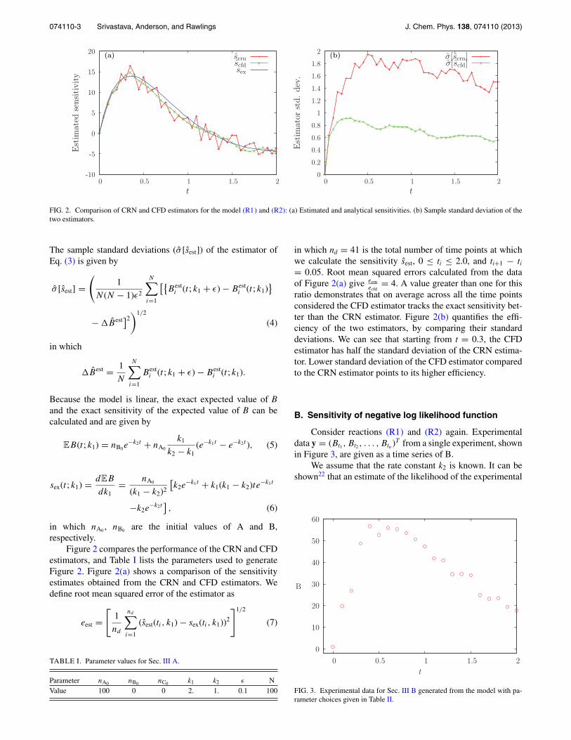
FIG. 2. Comparison of CRN and CFD estimators for the model (R1) and (R2): (a) Estimated and analytical sensitivities. (b) Sample standard deviation of thetwo estimators.
The sample standard deviations (σ [sest]) of the estimator ofEq. (3) is given by
σ [sest] =(
1
N (N − 1)ε2
N∑i=1
[{Best
i (t ; k1 + ε) − Besti (t ; k1)
}
− �Best]2
)1/2
(4)
in which
�Best = 1
N
N∑i=1
Besti (t ; k1 + ε) − Best
i (t ; k1).
Because the model is linear, the exact expected value of Band the exact sensitivity of the expected value of B can becalculated and are given by
EB(t ; k1) = nB0e−k2t + nA0
k1
k2 − k1(e−k1t − e−k2t ), (5)
sex(t ; k1) = dEB
dk1= nA0
(k1 − k2)2
[k2e
−k1t + k1(k1 − k2)te−k1t
−k2e−k2t
], (6)
in which nA0 , nB0 are the initial values of A and B,respectively.
Figure 2 compares the performance of the CRN and CFDestimators, and Table I lists the parameters used to generateFigure 2. Figure 2(a) shows a comparison of the sensitivityestimates obtained from the CRN and CFD estimators. Wedefine root mean squared error of the estimator as
in which nd = 41 is the total number of time points at whichwe calculate the sensitivity sest, 0 ≤ ti ≤ 2.0, and ti+1 − ti= 0.05. Root mean squared errors calculated from the dataof Figure 2(a) give ecrn
ecfd= 4. A value greater than one for this
ratio demonstrates that on average across all the time pointsconsidered the CFD estimator tracks the exact sensitivity bet-ter than the CRN estimator. Figure 2(b) quantifies the effi-ciency of the two estimators, by comparing their standarddeviations. We can see that starting from t = 0.3, the CFDestimator has half the standard deviation of the CRN estima-tor. Lower standard deviation of the CFD estimator comparedto the CRN estimator points to its higher efficiency.
B. Sensitivity of negative log likelihood function
Consider reactions (R1) and (R2) again. Experimentaldata y = (Bt1 , Bt2 , . . . , Btn )T from a single experiment, shownin Figure 3, are given as a time series of B.
We assume that the rate constant k2 is known. It can beshown22 that an estimate of the likelihood of the experimental
0
10
20
30
40
50
60
0 0.5 1 1.5 2
B
t
FIG. 3. Experimental data for Sec. III B generated from the model with pa-rameter choices given in Table II.
074110-4 Srivastava, Anderson, and Rawlings J. Chem. Phys. 138, 074110 (2013)
0
200
400
600
800
1000
1200
0 500 1000 1500 2000 2500 3000 3500 4000
i
(y − xi(k1)) R−1 (y − xi(k1))
(a)
10−250
10−200
10−150
10−100
10−50
100
0 500 1000 1500 2000 2500 3000 3500 4000
i
exp (−(1/2)(y − xi(k1)) R−1(y − xi(k1)))
(b)
10−160
10−140
10−120
10−100
10−80
10−60
10−40
0 500 1000 1500 2000 2500 3000 3500 4000
L(k
1,N
)
N
(c)
50
100
150
200
250
300
350
0 500 1000 1500 2000 2500 3000 3500 4000
φ
N
(d) φcrn(k1 + N)φcrn(k1, N)
-700
-600
-500
-400
-300
-200
-100
0
100
0 500 1000 1500 2000 2500 3000 3500 4000
s crn
(k1,N
)
N
(e)
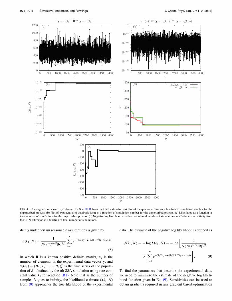
FIG. 4. Convergence of sensitivity estimate for Sec. III B from the CRN estimator: (a) Plot of the quadratic form as a function of simulation number for theunperturbed process. (b) Plot of exponential of quadratic form as a function of simulation number for the unperturbed process. (c) Likelihood as a function oftotal number of simulations for the unperturbed process. (d) Negative log likelihood as a function of total number of simulations. (e) Estimated sensitivity fromthe CRN estimator as a function of total number of simulations.
data y under certain reasonable assumptions is given by
L(k1, N ) = 1
N (2π )nd/2|R|1/2
N∑i=1
e−(1/2)(y−xi (k1))′R−1(y−xi (k1))
(8)
in which R is a known positive definite matrix, nd is thenumber of elements in the experimental data vector y, andxi(k1) = (Bt1 , Bt2 , . . . , Btn )Ti is the time series of the popula-tion of B, obtained by the ith SSA simulation using rate con-stant value k1 for reaction (R1). Note that as the number ofsamples N goes to infinity, the likelihood estimate L(k1, N)from (8) approaches the true likelihood of the experimental
data. The estimate of the negative log likelihood is defined as
φ(k1, N ) = − log L(k1, N ) = − log
[1
N (2π )nd/2|R|1/2
×N∑
i=1
e−(1/2)(y−xi (k1))′R−1(y−xi (k1))
]. (9)
To find the parameters that describe the experimental data,we need to minimize the estimate of the negative log likeli-hood function given in Eq. (9). Sensitivities can be used toobtain gradients required in any gradient based optimization
074110-5 Srivastava, Anderson, and Rawlings J. Chem. Phys. 138, 074110 (2013)
100
200
300
400
500
600
700
800
900
1000
1100
0 500 1000 1500 2000 2500 3000 3500 4000
i
(y − xi(k1)) R−1 (y − xi(k1))
(a)
10−250
10−200
10−150
10−100
10−50
100
0 500 1000 1500 2000 2500 3000 3500 4000
i
exp (−(1/2)(y − xi(k1)) R−1(y − xi(k1)))
(b)
10−110
10−100
10−90
10−80
10−70
10−60
10−50
10−40
0 500 1000 1500 2000 2500 3000 3500 4000
L(k
1,N
)
N
(c)
60
80
100
120
140
160
180
200
220
240
0 500 1000 1500 2000 2500 3000 3500 4000
φ
N
(d) φcfd(k1 + N)φcfd(k1, N)
-200
-180
-160
-140
-120
-100
-80
-60
0 500 1000 1500 2000 2500 3000 3500 4000
s cfd(k
1,N
)
N
(e)
FIG. 5. Convergence of sensitivity estimate for Sec. III B from the CFD estimator: (a) Plot of quadratic form as a function of simulation number for theunperturbed process. (b) Plot of exponential of quadratic form as a function of simulation number for the unperturbed process. (c) Likelihood as a function oftotal number of simulations for the unperturbed process. (d) Negative log likelihood as a function of total number of simulations. (e) Estimated sensitivity fromthe CFD estimator as a function of total number of simulations.
algorithm. Here, we are interested in the sensitivity
s(k1, N) = dφ(k1, N )
dk1(10)
of the estimated negative log likelihood function and the con-vergence of this sensitivity with the number of samples, N.The forward finite difference approximation of (10) is givenby
s(k1, N) ≈ φ(k1 + ε,N ) − φ(k1, N )
ε. (11)
We write estimator est ∈ {CRN, CFD} of the sensitivity s(k1,N) of Eq. (10) as
sest(k1, N ) = φest(k1 + ε,N ) − φest(k1, N )
ε(12)
in which φest(k1, N) is the estimate of the negative loglikelihood obtained from Eq. (9) using the estimator est ∈{CRN, CFD}.
Figure 4 shows the steps in obtaining the sensitivityof the negative log likelihood function using the CRN esti-mator. Table II contains the parameters used in this exam-ple. Figure 4(a) shows the variation of the quadratic form
074110-6 Srivastava, Anderson, and Rawlings J. Chem. Phys. 138, 074110 (2013)
(y − xi(k1))′R−1(y − xi(k1)) as a function of individual SSAsimulation number i. Figure 4(a) reveals the wide variation inthe value of the quadratic form for different individual SSAsimulations. Figure 4(b) is a plot of e−(1/2)(y−xi (k1))′R−1(y−xi (k1))
as a function of the individual SSA simulation number i. Thewide variation in (y − xi(k1))′R−1(y − xi(k1)) of Figure 4(a)leads to even wider variation in the exponential, as depictedin Figure 4(b). Figure 4(c) depicts convergence of L(k1, N)with N. L(k1, N) in Figure 4(c) is given by Eq. (8). Large vari-ation in e−(1/2)(y−xi (k1))′R−1(y−xi (k1)) as depicted in Figure 4(b)explains the sharp jumps in L(k1, N) which occur wheneverthe last SSA simulation i = n dominates all the previous 1 ≤ i≤ n − 1 simulations. Figure 4(d) shows the convergence of thenominal and perturbed negative log likelihoods: φcrn(k1, N)and φcrn(k1 + ε,N ). The sharp jumps in φcrn(k1, N) occur atthe same n values as the jumps in L(k1, N) in Figure 4(c).Finally, Figure 4(e) shows the convergence of the sensitiv-ity of the negative log likelihood using the CRN estimator,scrn(k1, N), as a function of N.
Next, we change focus from the CRN estimator to theCFD estimator. In Figures 5(a)–5(e), we plot the analogousresults to Figures 4(a)–4(e). Finally, Figure 6 compares con-vergence of CRN estimator, scrn(k1, N), and CFD estimator,scfd(k1, N). We see that the convergence of the CFD estima-tor to the estimated true value is faster than the CRN estima-tor. An estimated true value is obtained by performing 50 000simulations of the CFD estimator. The quicker convergenceproperty makes the CFD estimator a natural choice for the es-timator of sensitivity of negative log likelihood. One point tonote is that, as N → ∞, the final converged value for bothCFD and CRN estimators is going to be the same, becauseboth the estimators have the same bias; the CRN estimatorshown in Figure 6 simply has not converged by N = 4000.
-700
-600
-500
-400
-300
-200
-100
0
100
0 500 1000 1500 2000 2500 3000 3500 4000
N
scrn(k1, N)scfd(k1, N)
Exact
FIG. 6. Convergence of the estimated sensitivities of (11) from CRN andCFD estimators. Compared to the CRN estimator the CFD estimator showsquicker convergence to the estimated true value.
Regulatory Protein
g1
g2 g3
g4
r5
r3
r1
r7r6
r4
r8
r2
FIG. 7. Schematic diagram of the pap regulatory network. There are fourpossible states of the pap operon depending on the LRP-DNA binding.
C. Sensitivity of a rare state probability
Consider the pap operon regulation10, 23 which has a bi-ologically important rare state. In Srivastava et al.,23 we ob-tained a significantly better estimate of the rare state probabil-ity using stochastic quasi-steady-steady perturbation analysis(sQSPA), compared to both the full model and importancesampling based methods.24, 25 Figure 7 shows the schematicof the pap operon regulation.
State g1 is the rare state. The master equation for the sys-tem is
dP1
dt= −(r1 + r3)P1 + r2P2 + r4P3, (13)
dP2
dt= −(r2 + r5)P2 + r1P1 + r6P4, (14)
dP3
dt= −(r4 + r7)P3 + r3P1 + r8P4, (15)
dP4
dt= −(r6 + r8)P4 + r5P2 + r7P3, (16)
in which Pi(t; r2): i = 1, 2, 3, 4 is the probability of state gi
and rj: j = 1, 2, . . . , 8 are the rates of transition defined inTable III. Define
Si(t ; r2) = ∂Pi
∂r2i = 1, 2, 3, 4. (17)
The governing equations for the sensitivities Si: i=1,2,3,4 areobtained by differentiating (13)–(16) with respect to r2,
dS1
dt= −(r1 + r3)S1 + P2 + r2S2 + r4S3, (18)
dS2
dt= −P2 − (r2 + r5)S2 + r1S1 + r6S4, (19)
dS3
dt= −(r4 + r7)S3 + r3S1 + r8S4, (20)
dS4
dt= −(r6 + r8)S4 + r5S2 + r7S3. (21)
074110-7 Srivastava, Anderson, and Rawlings J. Chem. Phys. 138, 074110 (2013)
TABLE III. Reaction stoichiometry and reaction rates for Sec. III C.
In Srivastava et al.,23 we showed that the sQSPA modelreduction leads to the reaction network shown in Figure 8.
In the sQSPA model reduction, we write probabilities Pi:i = 1, 2, 3, 4 in a power series expression given by
Pi = Wi0 + εsqWi1 + ε2sqWi2 + O
(ε3
sq
),
in which εsq = 1r1+r3
. By comparing O(ε0sq) terms, the sQSPA
model reduction finds the expression for Wi0, i = 1, 2, 3, 4.The master equation for the sQSPA reduced model is
W10 = 0, (22)
dW20
dt= −[r1 + r5]W20 + r2W30 + r6W40, (23)
dW30
dt= −[r2 + r7]W30 + r1W20 + r8W40, (24)
dW40
dt= −[r6 + r8]W40 + r5W20 + r7W30, (25)
in which Wij are the jth-order probabilities of state gi: i = 1,2, 3, 4, r1 = r2r3/(r1 + r3), and r2 = r1r4/(r1 + r3). By com-paring O(ε1
sq) terms, one crucial equation23 that comes out isthe approximation of the probability (Psq1
) of the rare state interms of the probabilities of the other states satisfies
Psq1= εsq(r2W20 + r4W30) (26)
in which εsq = 1/(r1 + r3).
r1
r2
r6
r5 r8r7
g4
g3g2
FIG. 8. Reduced system of the pap regulatory network of Sec. III C in theslow time scale regime.
We are interested in the sensitivity of probability of therare state g1, with respect to r2,
s(t ; r2) = S1 = ∂P1(t ; r2)
∂r2. (27)
To estimate s(t; r2) of Eq. (27), we use three different estima-tors: CRN, CFD, and sQSPA with common random numbers(SRN). The CRN estimator is given as
scrn(t ; r2) = 1
Nε
N∑i=1
[1(pacrn
i (t, r2 + ε) = g1)
− 1(pacrn
i (t, r2) = g1)]
(28)
in which pacrni (t ; r2) is the state of the pap operon at time t
with rate parameter r2 obtained through the ith CRN simula-tion, and N is the number of CRN simulations. A point to noteis that the ith CRN simulation uses one SSA simulation withrate parameter r2, i.e., pacrn
i (t ; r2), and one SSA simulationwith rate parameter r2 + ε, i.e., pacrn
i (t ; r2 + ε). The indica-tor random variable 1(A) evaluates to 1 whenever the eventA happens and 0 otherwise. In an analogous fashion, we havethe CFD estimator for Eq. (27) as
scfd(t ; r2) = 1
Nε
N∑i=1
[1(pacfd
i (t, r2 + ε) = g1)
− 1(pacfd
i (t, r2) = g1)]
. (29)
The SRN estimator estimates the sensitivity of Psq1of Eq. (26)
with respect to r2. The SRN estimator is given by
ssrn = εsq
ε
[(r2 + ε)W20(t ; r2 + ε) + r4W30(t ; r2 + ε)
− r2W20(t ; r2) − r4W30(t ; r2)]
(30)
in which W20(t ; r2) and W20(t ; r2 + ε) are obtained by simu-lating the reduced system shown in Figure 8 and governed bythe master equation (22)–(25) using common random num-bers and SSA simulations. Figure 9 shows a comparison ofthe CRN, CFD, and SRN estimators. The ratio of root meansquared errors of CRN and CFD estimators is ecrn
ecfd= 4.75. As
the number of reaction events is small in the pap operon, wealso apply the likelihood gradient method.15 We performed500 simulations for each of the four estimators. The likeli-hood method performs better than both CRN and CFD forthis example, but it performs worse than SRN. The SRN es-timator tracks the true sensitivity closely except for a smallinitial time. This example reveals the distinct advantage ofanalytical insight and model reduction, e.g., the sQSPA anal-ysis, over the several proposed estimators that do not use thereduced model.
In this example, the number of reactions fired within thetime interval of consideration was small, which is preciselywhen the likelihood method can produce a low variance es-timator. In fact, in this particular application the likelihoodmethod even outperformed the CFD method. For models witheven a moderate number of reaction events, the likelihoodmethod will not outperform CFD. We also note that in this ex-ample, the SRN method outperforms all other methods. How-ever, SRN requires the ability to perform an analytic model
074110-8 Srivastava, Anderson, and Rawlings J. Chem. Phys. 138, 074110 (2013)
-0.04
-0.02
0
0.02
0.04
0.06
0 0.1 0.2 0.3 0.4 0.5
Est
imat
edse
nsi
tivity
t
(a) scrnscfdssrnslrs
0
0.005
0.01
0.015
0.02
0 0.1 0.2 0.3 0.4 0.5
Est
imat
edse
nsi
tivity
t
(b)
scfdssrnslrs
FIG. 9. Estimated sensitivity from the CRN, CFD, and SRN estimators for Sec. III C. The SRN estimator tracks the true sensitivity closely except for a smallinitial time. The CFD estimator performs better than the CRN estimator. On the right, we see that the likelihood method performs better than both the CRN andCFD methods but it performs worse than SRN.
reduction using sQSPA, which was possible in this example,thought not in general.
D. Sensitivity of a fast fluctuating species
In a stochastic simulation of the infection cycle of vesic-ular stomatitis virus (VSV), there is a fast fluctuation in a pro-tein at low copy number along with a rapid increase in thepopulation of the viral genome. Such a system is expensiveto simulate because the frequency of the fluctuation increasesas the simulation progresses leading to small time steps in theSSA simulation.26 To illustrate the phenomenon, consider thefollowing simple 3-species, 3-reaction system
A + Gk1−→ C + G, (R3)
C + Gk2−→ 2G + A, (R4)
2Gk3−→ G (R5)
with k2 ∼ k1 k3. This reaction system describes the interac-tion of three species in a simplified VSV replication process– two forms of viral polymerase, A and C, and viral genomeG. The two forms of the polymerase arise because VSV hastwo different complexes that serve as viral transcriptase and
replicase.27 The viral transcriptase form A is a complex ofconstituent VSV proteins L and P. The replicase form C is acomplex of L, N, and P proteins. The species A is involved inthe transcription reaction (R3) to produce messenger RNA.The transcription reaction leads to the conversion of tran-scriptase A into replicase C. We further assume that producedmRNA from reaction (R3) is short lived and hence we do notinclude it in the model. Species C and G are involved in repli-cation reaction (R4) to produce an additional viral genome G.The replication reaction (R4) leads to the conversion of repli-case C into transcriptase A. Finally, there is a second-orderdegradation reaction (R5) of the viral genome. The model(R3)–(R5) is insufficient to predict the full viral infection cy-cle, but it is instructive in understanding the simulation chal-lenges of the full infection cycle model used by Hensel et al.26
The reaction rate constants k1, k2, k3 denote macroscopic reac-tion rate constants with units μm3/(mol s). We express micro-scopic reaction rates in terms of macroscopic rate constants(k1, k2, k3) and the system size ,
r1 = 1
k1ag, r2 = 1
k2cg, r3 = 1
k3g(g − 1)
in which a, c, g represent the number of molecules of A,C, and G, respectively, and the system size appears be-cause the reactions are second order. For the purposes of this
0
1
2
3
0 1 2 3 4 5 6 7
c(t)
t (sec)
(a)(a)
100
101
102
103
104
105
106
0 1 2 3 4 5 6 7
g(t)
t (sec)
(b)
FIG. 10. A typical SSA simulation of the network of (R3)–(R5). (a) Counts of species C vs. time. (b) Counts of species G vs. time.
074110-9 Srivastava, Anderson, and Rawlings J. Chem. Phys. 138, 074110 (2013)
0
1000
2000
3000
4000
5000
6000
7000
8000
9000
0 1 2 3 4 5 6 7
Sta
ndar
ddev
iati
on
t
(a) σG[scrn]σG[scfd]
0
0.5
1
1.5
2
2.5
3
0 1 2 3 4 5 6 7
Sta
ndar
ddev
iati
on
t
(b)
σC[scrn]
σC[scfd]
FIG. 11. Comparison of standard deviations of CFD and CRN estimators for Sec. III D: (a) Species G and (b) Species C.
example, we take = 105μm3. A stochastic simulationwith the parameter values given in Table IV is shown inFigure 10. Species G increases continuously and this increaseforces species C to fluctuate with increasing frequency asshown in Figure 10.
We want to investigate the sensitivity
s(t ; k3) = dEX(t, k3)
dk3. (31)
In which X ∈ {C, G}. An estimator of the sensitivities of in-terest (31) is
sest = 1
N
N∑i=1
Xesti (t ; k3 + ε) − Xest
i (t ; k3)
ε(32)
in which est ∈ {CRN, CFD}. Figure 11 shows a comparisonof the standard deviations of the two estimators, CRN andCFD, obtained using Eq. (4). The parameters used to generateFigure 11 are shown in Table IV. Figure 11(a) shows that forthe abundant species G, CFD, and CRN estimators have sim-ilar standard deviations, which demonstrates that both CRNand CFD are capable of obtaining good sensitivity estimatesfor the abundant species G. Figure 11(b) shows that for fastfluctuating species C, the CFD estimator has less than onethird the standard deviation of the CRN estimator, whichdemonstrates that the CFD estimator captures the sensitivityof the fast fluctuating species C better than the CRN estimator.This example again demonstrates the superiority of the CFDestimator over the CRN estimator.
E. Sensitivity of genetic toggle switch
We conclude with a model of a genetic toggle switch1, 2, 28
and where XA(t) and XB(t) will denote the number of geneproducts from the two interacting genes. As in Refs. 1, 2,and 28, we take parameter values of b = 50, β = 2.5,a = 16, and α = 1. We consider the derivative of the expec-tation of XA with respect to α at the value one, with [XA(0),XB(0)] = [0, 0] as our choice of initial condition. We willconsider the behavior of three finite difference methods onthis example: CFD, CRN, and CRP.2 For each of the three fi-nite difference methods employed, we use a perturbation ofε = 1/50.
Figure 12 shows a comparison of the standard devia-tions of the three estimators. We again see the superiority ofthe CFD estimator over both the CRN and CRP estimators.
FIG. 12. Comparison of standard deviations of CFD, CRN, and CRP esti-mators on the model (33).
074110-10 Srivastava, Anderson, and Rawlings J. Chem. Phys. 138, 074110 (2013)
Further, starting at time t = 5s, the standard deviation of theCRN estimator is less than that of the CRP estimator. Thisresult demonstrates that it is not always the case that CRP issuperior to CRN, something not previously observed in theliterature.
IV. CONCLUSIONS
In this paper, we compared the performance of several fi-nite difference sensitivity estimators on a number of examplesnot previously considered in the literature. In all the exam-ples and sensitivities of interest, we found that the newly de-veloped CFD estimator performs significantly better than theCRN estimator, which is currently the most commonly usedmethod. Further, in Sec. III E we provided a case in which theCRN estimator is superior to the CRP estimator.
In previous work, it had been shown that the CFD es-timator performs better than the CRP estimator.1 The com-parisons made in this paper, along with Anderson’s previousresults, lead to the conclusion that CFD is currently the bestavailable estimator in the class of finite difference estimatorsof stochastic chemical kinetic models.
Estimating sensitivities of stochastic chemical kineticmodels accurately and efficiently remains an important prob-lem. With variance reduction ideas incorporated in the CFDestimator through a tight coupling of the nominal and per-turbed systems, we believe this estimator has significant ad-vantages over previous estimators without such a coupling.The CFD estimator has significant potential for application inparameter estimation where it can provide accurate estimatesof the Hessian of the objective function. Recently, Wolf andAnderson28 have also proposed a CFD2 estimator to directlyestimate the Hessian of the objective function. Evaluating theeffectiveness of CFD and CFD2 estimators in parameter es-timation of stochastic chemical kinetic models is a topic ofongoing research.
1D. F. Anderson, SIAM J. Numer. Anal. 50, 2237 (2012).2M. Rathinam, P. W. Sheppard, and M. Khammash, J. Chem. Phys. 132,034103 (2010).
3H. H. McAdams and A. Arkin, Proc. Natl. Acad. Sci. U.S.A. 94, 814(1997).
4A. Arkin, J. Ross, and H. McAdams, Genetics 149, 1633 (1998).5M. B. Elowitz, A. J. Levine, E. D. Siggia, and P. S. Swain, Science 297,1183 (2002).
6E. M. Ozbudak, M. Thattai, I. Kurtser, A. D. Grossman, and A. van Oude-naarden, Nat. Genet. 31, 69 (2002).
7W. J. Blake, M. A. Kaern, C. R. Cantor, and J. J. Collins, Nature (London)422, 633 (2003).
8J. M. Raser and E. K. O’Shea, Science 304, 1811 (2004).9S. Hooshangi, S. Thiberge, and R. Weiss, Proc. Natl. Acad. Sci. U.S.A.102, 3581 (2005).
10B. Munsky and M. Khammash, J. Chem. Phys. 124, 044104 (2006).11D. T. Gillespie, J. Phys. Chem. 81, 2340 (1977).12D. T. Gillespie, Physica A 188, 404 (1992).13J. B. Rawlings and J. G. Ekerdt, Chemical Reactor Analysis and Design
Fundamentals (Nob Hill, Madison, WI, 2004), p. 640.14P. W. Glynn, Commun. ACM 33, 75 (1990).15M. K. Nakayama, A. Goyal, and P. W. Glynn, Oper. Res. 42, 137
(1994).16S. Plyasunov and A. P. Arkin, J. Comput. Phys. 221, 724 (2007).17M. Komorowski, M. J. Costa, D. A. Rand, and M. P. H. Stumpf, Proc. Natl.
Acad. Sci. U.S.A. 108, 8645 (2011).18R. Gunawan, Y. Cao, L. Petzold, and F. J. Doyle, Biophys. J. 88, 2530
(2005).19P. W. Glynn, in Proceedings of the 21st Conference on Winter Simulation
(ACM, 1989), pp. 90–105.20J. McGill, B. Ogunnaike, and D. Vlachos, J. Comput. Phys. 231, 7170
(2012).21T. Drews, R. Braatz, and R. Alkire, J. Electrochem. Soc. 150, C807 (2003).22This will be a part of an upcoming publication.23R. Srivastava, E. L. Haseltine, E. A. Mastny, and J. B. Rawlings, J. Chem.
Phys. 134, 154109 (2011).24H. Kuwahara and I. Mura, J. Chem. Phys. 129, 165101 (2008).25M. K. Roh, D. T. Gillespie, and L. R. Petzold, J. Chem. Phys. 133, 174106
(2010).26S. Hensel, J. B. Rawlings, and J. Yin, Bull. Math. Biol. 71, 1671
(2009).27J. K. Rose and M. A. Whitt, in Fields Virology, 4th ed., edited by D. M.
Knipe and P. M. Howley (Lippincot, Philadelphia, 2001), Vol. 1, pp. 1221–1244.
28E. S. Wolf and D. F. Anderson, J. Chem. Phys. 137, 224112 (2012).