Abstract Fuzzy adaptive controllers can guarantee tightcontrol performance when the plant under control is uncer-tain and non-linear. Adaptive algorithm(s) which is an inte-gral component of the control strategy plays a significantrole in determining the control performance. In this work,the performance of a model-free fuzzy adaptive controller(MFFAC) is compared for two different variations of theadaptive algorithm. The adaptive fuzzy controller is mod-eled as a Takagi–Sugeno model. The MFFAC develops anonline inverse model of the plant. Adaptive algorithms basedon least mean square (LMS) are extensively used for onlinelearning. In this paper two variations of the LMS algo-rithm are compared. The two algorithms are normalized leastmean square and fuzzy least mean square. Both the adaptiveschemes were tested for different parameters of the adaptivefuzzy controller. The aim was to investigate the robustnessof the controller and the rate of convergence of the controllerparameters when the plant is subjected to noise and distur-bances.
Keywords Model-free adaptive control · Fuzzy identi-fication Schemes · Takagi–Sugeno models · Least squarelearning schemes
M. B. KadriElectronics and Power Engineering Department, PN EngineeringCollege, National University of Sciences and Technology,Islamabad, Pakistan
M. B. Kadri (B)PN Engineering College, Habib Ibrahim Rehmatullah Road,Karsaz, Karachi 75350, Pakistane-mail: [email protected]; [email protected]
1 Introduction
Control of non-linear and uncertain systems is a challengingtask. Gain scheduled control techniques have been appliedin the past which guarantee acceptable control performancefor a range of operating points. The control performance ofthese controllers degrades when the plant dynamics changeover the period of time and the gains need to be re-calculated[1,2]. Adaptive control with online and offline plant model-ing gives a better control performance due to the adaptation ofthe control parameters [3]. If the plant is modeled offline andcascaded with a model-based adaptive controller, then thecontrol performance can be compromised. The poor controlperformance of model-based adaptive controller is the resultof poor training in some regions due to the unavailability ofthe training data [1]. Online adaptation can be effectively uti-lized to adapt the model parameters with the changing plantdynamics [4]. Model-based control involves extra computa-tion due to the requirement of a plant model for controlling
123
Arab J Sci Eng
purpose [5]. Model-free controllers are best suited for uncer-tain and information poor systems. Fuzzy logic proposed byZadeh [6,7] when incorporated with adaptive control strate-gies can handle uncertainties. The adaptive algorithm whichis utilized in model-free controllers governs the control per-formance. If the adaptive algorithm has fast convergence androbust, then tight control performance can be guaranteed.
Least square approaches for adaptive learning and controlhave been extensively reported in literature [8–10]. If theproblem is formulated such that the square of the errors needto be minimized, then the least square approaches guaranteeconvergence to the optimal parameters [10,11]. A compari-son between fuzzy linear regression and ordinary least squareregression can be found in [12,13]. Due to the robust natureof the fuzzy least square algorithms, many variants of theleast square algorithm have been proposed [1,14].
In this paper, two variations of least mean square (LMS)algorithms are compared and discussed when they are usedto update the control parameters of the model-free adaptivefuzzy controller. The paper is organized as follows: the firstsection discusses the model-free fuzzy adaptive controller(MFFAC). NLMS and FLMS are elaborated in the next sec-tion. The plant on which the performance of the adaptiveschemes is compared is discussed in Sect. 4. Section 5 dis-cusses the impact of the adaptive schemes on the controlperformance when three control parameters are varied.
2 Model-Free Fuzzy Adaptive Fuzzy Control Structure
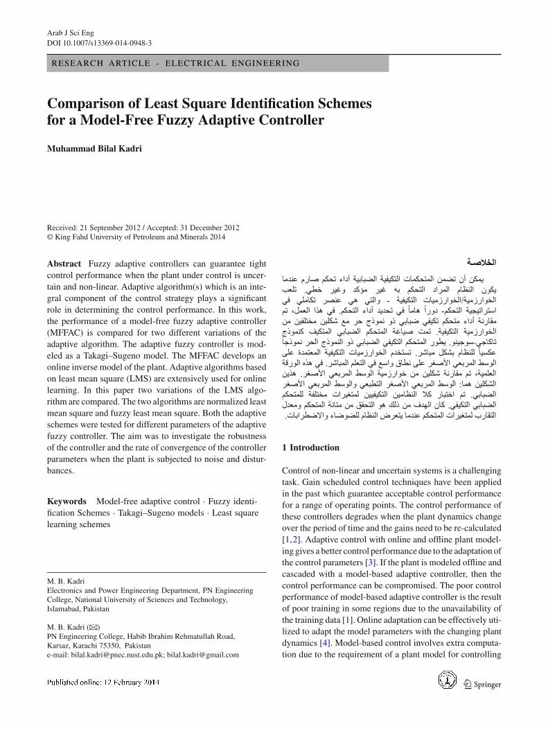
Model-free fuzzy adaptive controller is shown in Fig. 1.Model free implies that the controller does not explicitlybuild a model of the plant during the adaptation process.On the contrary, model based or indirect control strategiesbuild a model of the plant which is subsequently used toupdate the controller parameters [15,16]. The MFFAC hasbeen utilized in the control of different nonlinear processes,
such as cryogenic processes [17–19], cooling coil of an airhandling unit [20,21]. The feedback controller develops aninverse of the plant hence it is able to generate the correctcontrol signal which can derive the plant to the desired set-point. The feedback controller is a 0th order Takagi–SugenoModel. The feedback controller generates the control signalbased on the desired setpoint, feedback from the plant andthe weights (controller parameters) calculated by the fuzzyidentification algorithm. The fuzzy identification algorithmcomputes new weights at each sampling interval. If the fuzzyidentification scheme is good, then it guarantees weight con-vergence to the correct values, which consequently results intight control performance. On the contrary, if the fuzzy iden-tification scheme is numerically unstable or computationallydemanding, the weight convergence cannot be guaranteed.The weights are updated based on the prediction error ‘ε(t)’.The identification schemes reduce the ε(t) at each samplinginterval. ε(t) is the error between the control action com-puted from the old weights, i.e., weights at sampling interval‘t − 1’ and the estimated desired control action uf(t − 1) asshown in Eq. (1).
uf(t − 1) = uf(t − 1) + γ e(t) (1)
Equation (1) is termed as the feedback error learning law[22]. Feedback error learning law (FEL) is based on the rein-forcement learning technique [23]. ‘e(t)’ is the control errorcomputed between the plant output and the desired setpoint.γ is the learning rate and ‘uf(t − 1)’ is the control signalproduced by the feedback controller which resulted in thecontrol error e(t). The purpose of the FEL is to produce acontrol signal which will reduce the control error and forcethe plant towards the desired setpoint. The plant is assumed tobe monotonic. FEL law produces an estimate of the true con-trol action, which is subsequently used to compute the correctweights. The proportional controller in the MFFAC is used toguarantee acceptable control performance during the initialadaptation process when the fuzzy rule base is empty. The
Fig. 1 Block diagram of fuzzymodel reference adaptivecontroller
Fuzzy Identification
Algorithm
ProportionalController
Plant
FeedbackController
e(t)
r(t) u(t)ub(t)
uf(t)
+
-
+
+
MeasurableDisturbances
UnmeasuredDisturbances
Reference Model
123
Arab J Sci Eng
reference model is incorporated to make the desired setpointachievable.
3 Fuzzy Identification Schemes
The fuzzy identification schemes discussed in this paper aretwo different variations of the LMS algorithm. Normalizedleast mean square (NLMS) and fuzzy least mean square(FLMS) algorithms are the two variants in this category.
3.1 Normalized Least Mean Square Fuzzy Identification(NLMS)
Normalized least mean square algorithm [24] is suitable foronline learning because it is computationally undemanding.NLMS has been used as an efficient adaptive algorithm inthe field of signal processing [25] and neurofuzzy control[9,26,27]. It tries to minimize the error at every samplinginstant and is, therefore, very sensitive to noise. The NLMSupdate rule for the 0th order TS Fuzzy model is given by:
w(t) = w(t − 1) + δa(t)
aT (t)a(t)ε(t) (2)
where δ is the update rate,
ε(t) = uf(t) − uf(t) (3)
uf(t) = aT (t)w(t − 1) (4)
ε(t) is the prediction error, uf(t) is the estimates’ controlaction by the previous weight vector, w(t) is the currentweight vector and a(t) = a(x(t) = μA1s1
(x1(t) · μA2s2(x1(t)), . . . , μAnsn
(xn(t)))). ‘a(t)’ represents the rulestrength of the different rules fired by the incoming data.‘μ’ represents the individual membership grade.
3.2 Fuzzy Least Mean Square Fuzzy Identification (FLMS)
During online learning, the controller parameters are adaptedto the specific operating region. When the operating regionchanges, new rules are fired and consequently the weightvector is updated. There might be a possibility of learn-ing interference [9] which will corrupt the past learning.Consequently, the controller parameters need to be re-tuned when the controller returns to one of the operating
regions on which it was trained. To avoid re-training andto achieve robust learning, RSK learning scheme used withfuzzy relational models [28] is incorporated with NLMS.
RSK learning scheme was proposed by Ridley et al. [28]and has been applied to many control processes. RSKis used when the neurofuzzy controller is modeled as afuzzy relational model [29–31]. Recursive RSK is usedwhen the controller is used online. RSK is a very sim-ple, computationally undemanding scheme and is based onthe probabilistic modeling. The algorithm is defined for amulti-input single output system. A rule confidence matrixis formed which stores the mapping between the inputsx1(t), x2(t), . . . , xn(t) and the output y(t) where t is thesampling time. The entry RA1s1
,...,AnSn ,B j (t) in the fuzzyrelation array measures the possibility of obtaining an output‘y(t)’ in set ‘B j ’ from inputs x1(y), x2(t), . . . , xn(t) in setsA1S1
, . . . , Ansnrespectively. The input space of each vari-
able is divided into ‘r ’ referential sets using ‘r ’ fuzzy mem-bership functions. The fuzzy relational matrix is determinedby:
RA1s1,...,Ansn ,B j (t) =
∑Nk=1 f A1s1
,...,Ansn(x(t))μB j (y(t))
∑Nk=1 f A1s1 ,...,Ansn
(x(t)),
(5)
where f A1s1,...,A1s1
,...,Ansn(x(t)) is the product μA1s1
(x1(t)),
. . . , μAnsn(xn(t)) and the summation runs over the relevant
observations. The RSK scheme can be modified to weightthe data exponentially [32]. This will enable the recent datato have more impact on the rule confidences and to forget theold data.
RA1s1 ,...,Ansn ,B j (t)
=∑N
k=1 λN−k f A1s1,...,Ansn
(x(t))μB j (y(t))∑N
k=1 λN−k f A1s1 ,...,Ansn(x(t))
, (6)
where 0 < λ ≤ 1 is the forgetting factor and ‘N’ isthe number of times a particular combination of inputsets is fired. The RSK scheme can be converted intoa recursive form to save memory space and process-ing power. By defining an F Array of size
∏ni=1 Si ,
the denominator of Eq. (6) can be written in recursiveform:
FA1s1 ,...,Ansn(t) =
{
f A1s1 ,...,Ansn(x(t)) + λFA1s1 ,....Ansn
(t − 2) if f A1s1 ,...,Ansn(x(t �= 0))
FA1s1 ,...,Ansn(t − 1) otherwise
(7)
The F Array indicates the frequency with which a particularcombination of input has been fired. The recursive form ofthe RSK scheme is of the form:
123
Arab J Sci Eng
RA1s1 ,...,Ansn ,B j (t) =⎧
⎨
⎩
f A1s1,...,Ansn (x(t))μB j (y(t))+λRA1s1
,...,Ansn ,B j (t−1)FA1s1,...,Ansn (t−1)
FA1s1,...,Ansn (t) if f A1s1 ,...,Ansn
(x(t) �= 0)
RA1s1 ,...,Ansn ,B j (t − 1) otherwise(8)
The FLMS algorithm was proposed by [1,18] and has beensuccessfully applied to the control of non-linear processes[33–35]. The array S(t) in Eq. (9) is similar to the F(t) arrayof the RSK in Eq. (7). When a rule is fired, the correspondingF(t) value and hence the S(t) matrix is updated. A higherF(t) value indicates that the particular rule combination hasbeen fired many times.
w(t) = w(t − 1) + δS(t − 1)a(t − td)
aT (t − td)S(t − 1)a(t − td)ε(t) (9)
where δ is the update rate.
S(t) = diag{
S1, S2, . . . , Si , . . . , Sp}
(10)
si =p
∏
j=1, j �=1
Fj (t) (11)
Fi (t) = Fi (t − 1) + ai (t) (12)
ai (x(t)) = μA1i1(x1(t)) · μA2i2
(x2(t)), . . . , μAnin(xn(t)),
(13)
where ai (x(t)) is the strength with which the rule is fired
a(t) = [
a1a2, . . . , ap]
(14)
ε(t) = uf − aT (t − td)w(t − 1), (15)
where ε(t) is the prediction error.
4 Cooling Coil Modeled as a Hammerstein Model
The plant under consideration is a simplified model of thecooling coil of an air-conditioning unit. Many industrialprocesses can be approximated by a Hammerstein Model(a combination of a static non-linearity and linear dynam-ics). A cooling coil in an air-conditioning system can berepresented by such a model [36]. The transfer function inLaplace form is given by:
y(s) = L { f (u(t))} · e−sTd
τ s + 1, (16)
where ‘Td ’ is the dead time of the plant and ‘τ ’ is the timeconstant of the cooling coil. ‘u(t)’ determines the positionof the control valve and ‘y(s)’ is the Laplace transform ofthe temperature difference across the coil. The static non-linearity ‘ f (u)′ is defined as:
f (u) = 1
3.433ln(30u + 1) (17)
Td = 10 s and τ = 200 s in all of the simulations.
4.1 Identification of a 0th Order Takagi–Sugeno (TS)Model
When 0th order TS model is used to model, the feedfor-ward controller, FLMS and NLMS are used as the trainingscheme. The value of the update rate (δ) for FLMS is 0.01.A small value of update rate ensures that the weights areupdated in small steps and do not respond to noisy measure-ment by making a drastic change in the weights which willaffect the control performance. Feedback error learning witha learning rate (γ ) of 0.5 is used. This value of the learn-ing rate will respond to the control error quickly, a smallvalue (≈0.1) of gamma will take more time for convergenceof the control parameters (weights), whereas a higher value(≈1.0) will cause the controlled variable to have overshootsand undershoots which are undesirable. F array in FLMSis initialized to 10.0. F array in FLMS corresponds to thecovariance matrix in recursive least square algorithm [1]. Ifthe covariance matrix is initialized to a small value, then theweights will be updated very slowly and if the value of thecovariance matrix is chosen to be large, then the weightswill jump away quickly from their initial estimates [37]. Theweights (rule consequents) are initialized to 0.5. Since thecontroller has no prior knowledge, therefore, all the weightsare initialized to the same value. The input to the controlleris x(t) = [r(t), y(t − td)]. Both the inputs have five mem-bership functions with apexes at 0.0, 0.25, 0.5, 0.75, 1.0. Thereference model has a time constant of 200 s. Since the mainobjective is disturbance rejection and the setpoint remainsconstant, the reference model is chosen to have the sametime constant as that of the plant. The sampling time of thecontroller is 10 s. To compare the control performance, theroot mean square of the control error (RMSE) (y(t) − r(t))and the mean absolute value of the control activity (MAE)(u(t) − u(t − 1)) are calculated.
4.2 Control Objective and Disturbance Modeling
The control objective is setpoint tracking which variesbetween 0.25 and 0.75 with a time period of 4,000 samples.The controller along with the plant and sensor is shown inFig. 2. The senor dynamics is modeled as a first-order systemhaving a time constant of 1,000 s. The senor noise is gener-ated by a random number generator. The random number isnormally distributed with a zero mean (μ) and a standarddeviation (σ).
123
Arab J Sci Eng
Fig. 2 Block diagram of thecontrol loop
PlantMFFACr(t)
u(t) y(t)
e(t)
+
-
Reference Signal
Sensor
ym(t)
Fig. 3 Comparison of RMSEof the control error for variablesensor noise (σ )
0.1 0.2 0.3 0.4 0.5 0.6 0.7 0.8
0.075
0.08
0.085
0.09
0.095
0.1
0.105Comparison of RMSE of FLMS and NLMS
Standard deviation ( σ ) of sensor noise
RM
SE
of t
he c
ontr
ol e
rror
FLMS Seed =1
FLMS Seed =100
NLMS Seed =1
NLMS Seed =100
5 Comparison of the Control Performanceof the MFFAC
5.1 Impact of Sensor Noise (σ) on the Learning Schemes
The RMSE of the control error increases monotonically forboth the cases as shown in Fig. 3. FLMS is more robust inrejecting the sensor noise as compared to the NLMS algo-rithm. RMSE of the control error is lower in case of FLMSfor all the noise levels. This clearly demonstrates the abil-ity of FLMS in rejecting the sensor noise. The reason forthe robust performance is that, the FLMS maintains the S(t)matrix as shown in Eq. (13). The S(t) matrix is updated eachtime the rules are fired. When a rule is repeatedly fired, theS(t) matrix value for the specific rule becomes large. Largervalues of S(t) signify more confidence in the weight. Whenthe noisy data are presented, there is a little change in theweight and hence the performance is not compromised. Thisis not the case in NLMS in which the weights are updatedeach time the rule is fired. The MAE of the control erroris shown in Fig. 4. The control activity is higher, whenNLMS is used in the MFAC as compared to FLMS. Sincethe weights are continuously updated for noisy data in caseof NLMS, hence the control activity is higher for all noise
levels. As the sensor noise level is increased, the gap betweenthe NLMS and FLMS curves widens. This indicates thatthe performance of the MFAC with NLMS learning schemedegrades rapidly when noise is introduced into the system(Tables 1, 2).
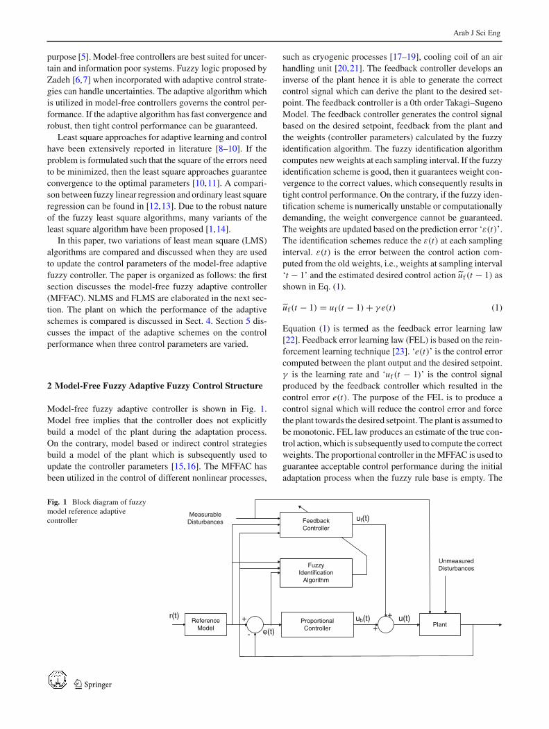
5.2 Impact of Forgetting Factor (λ) on the Learning Scheme
Forgetting factor defines the window length for the past data.If the value is near ‘1’, then the window size is bigger [18]which implies more past data are considered in the computa-tion of the new weights. The impact of increasing the forget-ting factor on the RMSE of the control error is shown in Fig. 5.For both the identification schemes, the RMSE is reducedwhich implies that the control performance improves whenthe forgetting factor is increased from 0 to 1. The improvedcontrol performance is the result of improved learning abil-ity and the convergence of the weights to the correct values.The MAE of the control activity is shown in Fig. 6. Ini-tially, the performance of NLMS is better as compared tothe FLMS learning scheme (control activity is lesser for λ =0.1), but when the forgetting factor is increased FLMS out-performs NLMS and has lower control activity with bettercontrol performance.
123
Arab J Sci Eng
Fig. 4 Comparison of MAE ofthe control error for variablesensor noise (σ )
0.1 0.2 0.3 0.4 0.5 0.6 0.7 0.82
3
4
5
6
7
8
9
10x 10
-4Comparison of MAE of FLMS and NLMS
Standard deviation ( ) of sensor noise
MA
E o
f the
con
trol
err
or
FLMS Seed =1
FLMS Seed =100
NLMS Seed =1
NLMS Seed =100
σ
Table 1 Comparison of RMSEof the control error for variablesensor noise (σ) for seed value= 1
SD OF SENSOR NOISE SEED = 1 SEED = 100
FLMS NLMS FLMS NLMS
0 8.7079E−02 9.4634E−02 7.4068E−02 9.4634E−02
0.1 8.7042E−02 9.4608E−02 7.4699E−02 9.5114E−02
0.2 8.7185E−02 9.4675E−02 7.5473E−02 9.5765E−02
0.3 8.7524E−02 9.4877E−02 7.6409E−02 9.6610E−02
0.4 8.8069E−02 9.5292E−02 7.7493E−02 9.7635E−02
0.5 8.8835E−02 9.5933E−02 7.8708E−02 9.8830E−02
0.6 8.9804E−02 9.6774E−02 8.0050E−02 1.0018E−01
0.7 9.0963E−02 9.7801E−02 8.1513E−02 1.0165E−01
0.8 9.2315E−02 9.9010E−02 8.3081E−02 1.0324E−01
0.9 9.3846E−02 1.0038E−01 8.4750E−02 1.0495E−01
Table 2 Comparison of MAEof the control error for variablesensor noise (σ ) for seedvalue= 1
SD OF SENSOR NOISE SEED = 1 SEED = 100
FLMS NLMS FLMS NLMS
0 1.8824E−04 2.1035E−04 1.9037E−04 2.1035E−04
0.1 2.4141E−04 2.8867E−04 2.6745E−04 2.8880E−04
0.2 3.0023E−04 3.7581E−04 3.0606E−04 3.7643E−04
0.3 3.6082E−04 4.6586E−04 3.8528E−04 4.6717E−04
0.4 4.2520E−04 5.5942E−04 4.5595E−04 5.6222E−04
0.5 4.9611E−04 6.5638E−04 5.1955E−04 6.6110E−04
0.6 5.7241E−04 7.5412E−04 5.9998E−04 7.6294E−04
0.7 6.5286E−04 8.4985E−04 6.9314E−04 8.6654E−04
0.8 7.3642E−04 9.4151E−04 7.7069E−04 9.7067E−04
0.9 8.2049E−04 1.0291E−03 8.5209E−04 1.0767E−03
123
Arab J Sci Eng
Fig. 5 Comparison of RMSEof the control error for variableforgetting factor (λ)
0.1 0.2 0.3 0.4 0.5 0.6 0.7 0.80.06
0.08
0.1
0.12
0.14
0.16
0.18
0.2Comparison of RMSE of FLMS and NLMS
Forgetting factor λ
RM
SE
of t
he c
ontr
ol e
rror
FLMS
NLMS
Fig. 6 Comparison of MAE ofthe control error for variableforgetting factor (λ)
0.1 0.2 0.3 0.4 0.5 0.6 0.7 0.81.5
1.6
1.7
1.8
1.9
2
2.1
2.2x 10
-4 Comparison of MAE of FLMS and NLMS
Forgetting factor λ
MA
E o
f the
con
trol
err
or
FLMS
NLMS
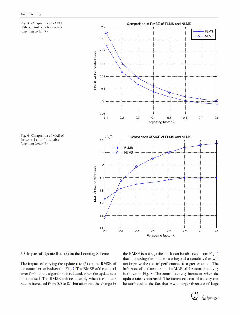
5.3 Impact of Update Rate (δ) on the Learning Scheme
The impact of varying the update rate (δ) on the RMSE ofthe control error is shown in Fig. 7. The RMSE of the controlerror for both the algorithms is reduced, when the update rateis increased. The RMSE reduces sharply when the updaterate in increased from 0.0 to 0.1 but after that the change in
the RMSE is not significant. It can be observed from Fig. 7that increasing the update rate beyond a certain value willnot improve the control performance to a greater extent. Theinfluence of update rate on the MAE of the control activityis shown in Fig. 8. The control activity increases when theupdate rate is increased. The increased control activity canbe attributed to the fact that �w is larger (because of large
123
Arab J Sci Eng
Fig. 7 Comparison of RMSEof the control error for variableupdate rate (δ)
0 0.05 0.1 0.15 0.2 0.25 0.3 0.350.03
0.04
0.05
0.06
0.07
0.08
0.09
0.1Comparison of RMSE of FLMS and NLMS
Update Rate δ
RM
SE
of t
he c
ontr
ol e
rror
FLMS
NLMS
Fig. 8 Comparison of MAE ofthe control error for variableupdate rate (δ)
0 0.05 0.1 0.15 0.2 0.25 0.3 0.351.8
2
2.2
2.4
2.6
2.8
3
3.2
3.4x 10
-4 Comparison of MAE of FLMS and NLMS
Update Rate δ
MA
E o
f the
con
trol
err
or
FLMS
NLMS
values of δ) at each instant which translates into larger controlactivity and improved control performance (as demonstratedby the RMSE). It can be observed from the figures that FLMShas much superior performance as compared to the NLMSboth in terms of control activity and control error. FLMSoffers good control performance (i.e., lower RMSE values)with low minimum control activity as compared to NLMS(Tables 3, 4).
6 Conclusions
The adaptation capability of a MFFAC is investigated in thispaper. Two different versions of the LMS algorithms, namelyFLMS and NLMS, were compared. Hammerstein model witha static non-linearity is used as the plant. The performance ofthe two adaptive algorithms was compared for three differ-ent parameters of the adaptive controller. Simulations were
123
Arab J Sci Eng
Table 3 Comparison of RMSE of the control error for variable updaterate (δ)
δ FLMS NLMS
0.01 0.087078891 0.094633847
0.05 0.051312395 0.055652021
0.1 0.043256527 0.047108488
0.15 0.039926789 0.043613699
0.2 0.03807111 0.041676666
0.25 0.036884929 0.040446935
0.3 0.036062154 0.039606665
0.35 0.035463917 0.039008209
Table 4 Comparison of MAE of the control error for variable updaterate (δ)
δ FLMS NLMS
0.01 1.8824E−04 2.1035E−04
0.05 2.1402E−04 2.5247E−04
0.1 2.3425E−04 2.7675E−04
0.15 2.4915E−04 2.9300E−04
0.2 2.6178E−04 3.0399E−04
0.25 2.7302E−04 3.1307E−04
0.3 2.8276E−04 3.2141E−04
0.35 2.9050E−04 3.2917E−04
performed to compare the control performance when forget-ting factor (λ), sensor noise (σ) and update rate of the adap-tive algorithm (δ) were varied. It was successfully demon-strated that the performance of FLMS was superior to itscounterpart in most of the cases. Both the algorithms werecompared on the basis of RMSE of the control error and MAEof the control activity. The adaptive controller has a lowervalue of RMSE and MAE when FLMS is used as the adap-tive scheme. It can be concluded that FLMS offers robustcontrol performance as well as fast weight convergence ascompared to NLMS.
Acknowledgments The research work was conducted in the ControlLaboratory, Department of Engineering Science, University of Oxford,U.K. under the supervision of Professor Arthur Dexter. The researchwas jointly funded by Higher Education Commission (HEC) and theNational University of Sciences and Technology (NUST), Islamabad,Pakistan.
References
1. Tan, W.-W.: An on-line modified least-mean-square algorithm fortraining neurofuzzy controllers. ISA Trans. 46, 181–188 (2007)
2. Dubay, R.; Kember, G.C.; Blanchett, T.P.: PID gain schedulingusing fuzzy logic. ISA Trans. 39, 317–325 (2000)
3. Santos, M.; Brandizzi, J.; Dexter, A.L.: Control of a cryogenicprocess using a fuzzy PID scheduler. In: Proceedings of the IFAC
Workshop on Digital Control:Past, Present and Future of PID Con-trol, Terassa, Spain pp. 401–405 (2000)
4. Rojas, I.; Pomares, H.; Gonzalez, J.; Herrera, L.J.; Guillen, A.;Rojas, F.; Valenzuela, O.: Adaptive fuzzy controller: applicationto the control of the temperature of a dynamic room in rael time.Fuzzy Sets Syst. (2006)
6. Zadeh, L.A.: Fuzzy sets. Inf. Control 8, 338–353 (1965)7. Procyk, T.J.; Mamdani, E.H.: A linguistic self-organizing process
controller. Automatica 15, 15–30 (1979)8. Stahl, C.: A strong consistent least-squares estimator in a linear
fuzzy regression model with fuzzy parameters and fuzzy dependentvariables. Fuzzy Sets Syst. 157, 2593–2607 (2006)
9. Brown, M.; Harris, C.J.: Neurofuzzy Adaptive Modelling and Con-trol. Prentice Hall International (1994)
10. Widrow, B.: Walach, E.: Adaptive Inverse Control. Prentice HallInformation & System Sciences Series (1996)
11. Wunsche, A.; Nather, W.: Least squares fuzzy regression with fuzzyrandom variables. Fuzzy Sets Syst. 130, 43–50 (2002)
12. Redden, D.T.; Woodall, W.H.: Properties of certain fuzzy linearregression methods. Fuzzy Sets Syst. 64, 361–375 (1994)
13. Yang, M.S.: Lin, T.S.: Fuzzy least-squares linear regression analy-sis for fuzzy input-output data. Fuzzy Sets Syst. 126, 389–399(2002)
14. Tang, M.S.; Liu, H.H.: Fuzzy least squares algorithms for interac-tive fuzzy linear regression models. Fuzzy Sets Syst. 135, 305–316(2003)
15. Sousa, J.M.d.C.: A Fuzzy Approach to Model-Based Control. Lis-bon, Portugal (1998)
16. Babuska, R.; Sousa, J.M.; Verbruggen, H.B.: Model based design offuzzy control systems. In: Proceedings 3rd European Congress OnIntelligent Techniques and Soft Computing (EUFIT ’95), Aachen,Germany, pp. 837–841 (1995)
17. Tan, W.W.; Dexter, A.L.: Self-learning neurofuzzy control of aliquid helium cryostat. Control Eng. Pract. 7, 1209–1220 (1999)
18. Tan, W.W.: Self-Learning Neurofuzzy Control of Non-Linear Sys-tems. D.Phil Thesis, University of Oxford (1997)
19. Santos, M.; Dexter, A.L.: Temperature control in liquid heliumcryostat using self-learning neurofuzzy controller. IEE Proc. Con-trol Theory Appl. 148, 233–238 (2001)
20. Thompson, R.; Dexter, A.L.: A fuzzy decision-making approachto temperature control in air-conditioning systems. Control Eng.Pract. 13, 689–698 (2005)
21. Kadri, M.B.: System identification of a cooling coil using recurrentneural networks. Arab. J. Sci. Eng. 37, 2193–2203 (2012)
22. Tan, W.W.; Lo, C.H.: Development of feedback error learningstrategies for training neurofuzzy controllers on-line. IEEE Int.Fuzzy Syst. Conf. 1016–1021 (2001)
23. Kawato, M.; Uno, Y.; Isobe, M.; Suzuki, R.: Hierarchical neuralnetwork model for voluntary movement with application to robot-ics. IEEE Control Syst. Mag. 8(2), 8–15 (1988)
24. Rogers, E.; Li, Y.: Parallel Processing in a Control Systems Envi-ronment. Prentice Hall (1993)
25. Cho, H.; Lee, C.W.; Kim, S.W.: Derivation of a new normalizedleast mean squares algorithm with modified minimization criterion.Signal Process. 89, 692–695 (2009)
26. Brown, M.; Mills, D.J.; Harris, C.J.: The representation of fuzzyalgorithms used in adaptive modelling and control schemes. FuzzySets Syst. 79, 69–91 (1996)
27. Kadri, M.B.; Dexter, A.L.: Disturbance rejection in information-poor systems using an adaptive model-free fuzzy controller. In:presented at Annual Meeting of the North American Fuzzy Infor-mation Processing Society, NAFIPS (2009)
123
Arab J Sci Eng
28. Ridley, J.N.; Shaw, I.S.: Kruger, J.J.: Probabilistic fuzzy model fordynamic systems. Electron. Lett. 24(14), 890–892 (1988)
29. Tan, W.W.; Dexter, A.L.: Properties of a Fuzzy Relational Model.Technical Report OUEL 2119/96. University of Oxford, Depart-ment of Engineering Science (1996b)
30. Kadri, M.B.; Hussain, S.: Model free adaptive control based onFRM with an approach to reduce the control activity. In: presentedat 2010 IEEE International Conference on Systems Man and Cyber-netics (SMC), Istanbul, Turkey (2010)
31. Kadri, M.B.: Robust model free fuzzy Adaptive controller withfuzzy and crisp feedback error learning schemes. In: Presented at12th International Conference on Control, Automation and Sys-tems (ICCAS), 2012, Jeju, South Korea (2012)
32. Postlethwaite, B.E.: Empirical comparisons of methods of a fuzzyrelational identification. IEE Proc. 138, 199–206, (1991)
33. Kadri, M.B.: Disturbance Rejection in Information Poor SystemsUsing Model Free Neurofuzzy Control. D.Phil Thesis, Universityof Oxford, (2009)
34. Kadri, M.B. Disturbance rejection in nonlinear uncertain systemsusing feedforward control. Arab. J. Sci. Eng. (2012)
35. Kadri, M.B.: Disturbance rejection in model free adaptive con-trol using feedback. In: presented at Modelling, Identification, andControl-2010, Innsbruck, Austria (2010)
36. Wang, S.W.: Dynamic simulation of building VAV air-conditioningsystem and Evaluation of EMCS On-line Control Strategies. Build.Environ. 34, 681–705 (1999)