Comparison of Model Order Reduction Methods for …2018 EngineeringOptimization...

March 26, 2018 Engineering Optimization MOR_Sensorplacement_EO

To appear in Engineering OptimizationVol. 00, No. 00, Month 20XX, 1–21

Comparison of Model Order Reduction Methods for Optimal SensorPlacement for Thermo-Elastic Models ∗

Peter Bennera,b, Email: [email protected],Roland Herzogc, Email: [email protected],Norman Langb, Email: [email protected],

Ilka Riedelc, Email: [email protected],Jens Saaka,b,∗∗, Email: [email protected].

aMax Planck Institute for Dynamics of Complex Technical Systems, Computational Methods inSystems and Control Theory, D–39106 Magdeburg, Germany;

bTechnische Universität Chemnitz, Faculty of Mathematics, Research Group Mathematics inIndustry and Technology, D–09107 Chemnitz, Germany

cTechnische Universität Chemnitz, Faculty of Mathematics, Professorship NumericalMathematics (Partial Differential Equations), D–09107 Chemnitz, Germany;

(October 2017)

In this paper we consider an optimal sensor placement problem for a thermo-elastic solid bodymodel. Temperature sensors are placed in a near-optimal way so that their measurementsallow an accurate prediction of the thermally induced displacement of a point of interest(POI). Low-dimensional approximations of the transient thermal field are used which allowfor efficient calculations. Four model order reduction (MOR) methods are applied and alsocompared with respect to the accuracy of the estimated POI displacement and the locationof the sensors obtained.

Keywords: thermo-elastic model; optimal sensor placement; model order reduction

1. Introduction

This paper is concerned with an optimal sensor placement problem for thermo-elasticsolid body models. The goal is to place temperature sensors in a near-optimal way so thattheir measurements allow an accurate prediction of the thermally induced deformation ata particular point of interest (POI) in real time. Our main motivation and example usedthroughout the paper is the prediction of the deflection of the tool center point (TCP)of a machine tool under thermal loading.Sensor placement problems for partial differential equations (PDEs) are difficult opti-

mization problems due to their large scale and the intricate structure of the objective,which normally involves the estimator covariance matrix of the quantity estimated, orits asymptotic inverse, the Fisher information matrix. In our approach we exploit theparticular structure of thermo-elastic models. While the evolution of the temperature Tis relatively slow, the deformation u is instantaneous. Moreover, we can neglect mechan-ically induced heat sources, so that the coupling is T 7→ u is uni-directional.

∗ An abridged version of the manuscript was submitted to the CIRP sponsored conference on Conference onThermal Issues in Machine Tools, 2018.∗∗Corresponding author.

1


In the optimal sensor placement problem, our objective is to choose sensor locationsin such a way that the measurements contain the maximum amount of information withregard not to the reconstruction of the temperature field itself, but rather with regard tothe subsequent prediction of the thermally induced displacement at a point of interest. Inorder to reduce the complexity of the placement problem we apply model order reduction(MOR) for the temperature field. In this paper we compare four model order reductiontechniques, namely Proper Orthogonal Decompositon (POD), Balanced Truncation (BT)and two different Moment Matching (MM) approaches. The focus of this paper is theapplication of modern model order reduction methods to the sensor placement procedure.Furthermore the results of the sensor placement for these different MOR methods for theunderlying temperature dynamics are compared.Let us put our work into perspective. Model order reduction techniques are frequently

used in sensor placement problems involving PDEs. We mention reaction-diffusion orconvection-diffusion problems (Alonso, Frouzakis, and Kevrikidis (2004); Green (2006);Armaou and Demetriou (2006); Alonso et al. (2004); García et al. (2007)) as well as fluiddynamics applications (Mokhasi and Rempfer (2004); Cohen, Siegel, and McLaughlin(2006); Willcox (2006); Yildirim, Chryssostomidis, and Karniadakis (2009)), where PODis often the method of choice. In another class of applications involving mechanical de-formation of large structures (Kammer (1991); Yi, Li, and Gu (2011); Meo and Zumpano(2005); Sun and Büyüköztürk (2015)), modal analysis is employed as a reduction tech-nique.The references above fall into three categories concerning the actual placement strategy,

viz. forward, backward and simultaneous placement procedures. In the forward sequentialsetting, which we also adopt, sensors are placed one by one such that one obtains amaximal gain of information for each sensor. In the backward approach, one begins witha set of all possible sensor locations and sequentially removes the ones which contributethe least amount of information. Both are greedy algorithms. Simultaneous placementprocedures can only be used, due to the combinatorial complexity, when the number ofpotential locations is relatively small.The goal in all of the above references is to reconstruct the respective field of the under-

lying PDE from a limited number of measurements. In our setting, this would correspondto recovering the entire temperature field from a number of temperature measurements.By contrast, the objective in this paper is to predict the mechanical displacement inducedby that temperature field. This approach changes the metric w.r.t. which we measure thegain of information; see Körkel et al. (2008), Koevoets et al. (2007) and Herzog and Riedel(2015). In Koevoets et al. (2007), thermally induced displacements are estimated usingtemperature measurements as well. However, in contrast to our work, only a small num-ber of potential sensor locations is considered, and modal analysis is used. In Herzog andRiedel (2015), we presented a sensor placement approach based on POD. One drawbackof this simulation based MOR technique is its dependence on the thermal load cycle usedto obtain the snapshots. The present paper is an extension of this work and we comparefour different MOR techniques, three of which do not depend on simulations and are thusmore widely applicable.The paper is organized as follows. In the remainder of this section we state the thermo-

elastic model. The sequential placement strategy is described in detail in section 3. Themodel order reduction techniques under consideration are presented in section 4. Numer-ous numerical experiments are provided in section 5 which allow a comparison of theMOR techniques in the context of sensor placement problems.

We introduced a separate section describing the model.

2


2. Thermo-Elastic Forward Model

Before describing the sensor placement and model order reduction procedures, we firstintroduce the model problem to be considered. We denote the solid body whose thermo-mechanical displacement we consider by Ω, and its surface by Γ. In our application Ω isthe column of a machine tool shown in Figure 1(a). We consider the linear heat equation,

ρ cp T − div(λ∇T ) = 0 in Ω× (0, tend),

λ∂

∂nT + α(x) (T − Tref) = r(x, t) on Γ× (0, tend),

T (·, 0) = T0 in Ω.

(1)

The boundary conditions represent a simple model for the free convection occuring at thesurface Γ, and the heat transfer coefficient may vary across the surface. The right handside r(x, t) represents thermal loads, e.g., due to electric drives. All symbols occuring in(1) are summarized in Table 1.

(a) Photograph of the machine col-umn.

(b) CAD model of the machine column.

Figure 1. Auerbach ACW 630 machine column.

Applying a standard linear Lagrangian finite element discretization in space, seee.g. Braess (2007); Grossmann, Roos, and Stynes (2007), the thermal boundary valueproblem (1) can be written in terms of a linear time-invariant (LTI) control system

EthT = AthT +Bthz,

T (·, 0) = T0.(2)

Here T ∈ Rnth represents the temperature field in the nodal Lagrangian basis. The so-called system inputs z ∈ Rm represent all external influences to the system such as thetemperatures Tref of the surrounding media and the thermal loads r(x, t). The matricesEth, Ath ∈ Rnth×nth , and Bth ∈ Rnth×m denote the mass matrix, the stiffness matrix, andthe input matrix, respectively.

3


The linear elasticity model is based on the balance of forces,

− divσ(ε(u), T ) = f in Ω. (3)

We employ an additive split of the stress tensor σ into its mechanically and thermallyinduced parts. Together with the usual homogeneous and isotropic stress-strain relation,we obtain the following constitutive law, see (Boley and Weiner 1960, Sec. 1.12), (Eslamiet al. 2013, Sec. 2.8):

σ(ε(u), T ) = σel(ε(u)) + σth(T ),

σel(ε(u)) =E

1 + νε(u) +

Eν

(1 + ν)(1− 2ν)trace(ε(u)) I,

σth(T ) = − E

1− 2νβ (T − Tref) I.

(4)

Herein, ε denotes the linearized strain tensor,

ε(u) =1

2(∇u+∇u>),

and I the 3×3 identity tensor. Moreover, E and ν denote Young’s modulus and Poisson’sratio; see Table 1.

Symbol Meaning Value Units

T temperature KT0 initial temperature Kr thermal surface load W m−2

ρ density 7 250 kg m−3

cp specific heat at constant pressure 500 J kg−1 K−1

λ thermal conductivity 46.8 W K−1 m−1

Tref ambient temperature 20 Cα heat transfer coefficient 0 to 12 W K−1 m−2

u displacement mσ stress N m−2

ε strain 1

ν Poisson’s ratio 0.3 1E modulus of elasticity 114·109 N m−2

β thermal volumetric expansion coefficient 1.1·10−5 K−1

Table 1. Table of symbols occuring in the thermal (1) and the elasticity model (4).

In order to simplify the notation, we consider from now on the temperature relativeto the constant Tref, i.e., we write T instead of T − Tref. Using the same finite elementdiscretization as for the thermal model (1) and noting that there are no further externalforces in the system, i.e., f = 0, system (3) becomes

Aelu−AthelT = 0, (5)

where u ∈ Rnel is the coefficient vector representing the spatially discretized displacementfield and the matrices Ael ∈ Rnel×nel and Athel ∈ Rnel×nth denote the elasticity stiffness

4


matrix and the thermo-elastic coupling matrix, respectively. Note that since we use thesame piecewise linear finite element (FE) discretization for both the thermal and elas-ticity equations, we have nel = 3nth. Since we are interested in the thermally induceddeformations of the machine column, we consider the coupling of the thermal model (2)with the elasticity equation (5) and obtain the coupled thermo-elastic system[

Eth 00 0

][Tu

]=

[Ath 0Athel −Ael

][Tu

]+

[Bth0

]z,

⇔ Ex = Ax+Bz

(6)

for the combined state x = (T, u), which is of dimension n = nth + nel = 4nth. Note thatthe coupled thermo-elastic model (6) and the thermal model (2) are basically of the sameform. Moreover, the coupled system is a so-called differential algebraic equation (DAE)of index 1. However, since we are interested in determining the displacement u at certainpoints of interest, specifically the tool center point in our application, we additionallydefine the output equation

y = Cx, (7)

where C ∈ Rq×n maps the state vector x to the points of interest, the so-called systemoutputs y. Finally, the thermo-elastic model is described by the LTI control system (6)–(7). In the following section, we present the sensor placement procedure based on thismodel.

3. Sequentially Optimal Sensor Placement

With the sensor placement problem we seek to choose optimal positions of temperaturesensors on the surface Γ. The goal is to reconstruct from these measurements the temper-ature field T as an intermediate quantity, and subsequently to predict the displacementu(xTCP) at the point of interest, i.e., the tool center point (TCP). As was mentionedin the introduction such placement problems are challenging for a number of reasons.In the following subsections, we reduce the complexity of the problem step by step sothat it becomes tractable. The material in this section closely follows (Herzog and Riedel2015, Sec. 2), where a sequential placement approach was proposed in the context of POD-reduced temperature dynamics. Major parts of this technique can be used in combinationwith other MOR methods as well. In the interest of keeping this paper self-contained,however, we briefly recall the main steps.

3.1 Displacement Estimation

Our first step to make the problem tractable is to apply model order reduction to thetemperature state space. That is, we replace the temperature T by an approximation

T ≈ V T ,

where V ∈ Rn×r with r n. The particular choice of the matrix V depends on themodel order reduction technique; see section 4. Exploiting the linearity of the elasticity

5


equation (5), we can express the elasticity field in terms of the reduced temperature T ,

u = S T ≈ S V T .

Herein, S = A−1el Athel is the solution operator for the elasticity equation. Then the dis-

placement at the point of interest is

u(xTCP) = Cel u ≈ Cel S V T ∈ R3 (8)

with an observation matrix Cel ∈ R3×nel which is related to the output equation y = Cxin (7) by

C =

[Cth 00 Cel

]with Cth ∈ Rqth×nth . Since in the present application only the displacement of the TCPis observed, we have qth = 0 and C = [0, Cel] holds.To estimate the TCP displacement (8) from temperature measurements, we first esti-

mate the reduced temperature T . This estimation will be instantaneous, i.e., at any givenmoment in time we estimate the temperature field using only measurements from thattime instance. Therefore we suppress the dependence on time in our notation. The esti-mation of the reduced temperature field is achieved by solving the least squares problem

MinimizeT∈Rr

1

2

nsensors∑i=1

(r∑

j=1

Tj vj(xi)− Ti

). (9)

Here Ti denotes the i-th temperature measurement, acquired at location xi on the sur-face Γ, where i = 1, . . . , nsensors. We restrict these locations to the vertices of the finiteelement mesh on the surface. Notice moreover that each row of the reduced basis matrixV corresponds to one nodal degree of freedom in the temperature finite element space.Hence we can identify the j-th column of V with a function vj . This justifies the notationvj(xi) = Vij .Next let X = [x1, · · · , xnsensors ] be the vector of all sensor positions selected. Then the

solution of the linear least-squares problem (9) is given by the normal equation

J(X)>J(X) T = J(X)>T . (10)

Here J(X) denotes the Jacobian of the residuals w.r.t. the unknowns (the components ofthe reduced temperature T ), i.e.,

J(X) =

v1(x1) · · · vr(x1)...

...v1(xnsensors) · · · vr(xnsensors)

∈ Rnsensors×r.

The vector of measurements is

T = [T1, · · · , Tnsensors ]>.

The solution of (10) is unique if J(X) has full rank, which we assume. To ensure this,it is necessary to have nsensors ≥ r. The solution of (10) provides an estimator for the

6


reduced temperature,

θT (X) =(J(X)>J(X)

)−1J(X)>T .

Using the relation (8), an estimator for the TCP displacement u(xTCP) is given by

θu(xTCP)(X) = CelSV θT (X) = CelSV(J(X)>J(X)

)−1J(X)>T . (11)

3.2 Covariance of the Estimator

In order to assess the quality of the estimator we consider the covariance matrix ofθu(xTCP)(X). We assume the measurement errors to be i.i.d. random variables with normaldistribution N (0, µ2), i.e., with zero mean and the variance µ2. This means that themeasurements T are normally distributed with associated covariance matrix

CovT = µ2I.

The estimator θT (X) for the reduced temperature field is a linear transformation of themeasurements T , thus its covariance can be written as

CovT (X) =(J(X)>J(X)

)−1J(X)>CovT J(X)

(J(X)>J(X)

)−1

= µ2(J(X)>J(X)

)−1 ∈ Rr×r.

Analogously we obtain the covariance of the estimator θu(xTCP)(X) for the TCP displace-ment from

Covu(xTCP)(X) = µ2CelSV(J(X)>J(X)

)−1(CelSV )> ∈ R3×3. (12)

Notice that the covariance Covu(xTCP)(X) does not depend on the current thermal stateof the machine. However it does depend on the sensor positions selected (encoded in X)as well as on the choice of the reduced-order basis matrix V .

3.3 Sensor Placement Strategy

The precision of a linear least-squares estimator can be inferred from the eigenvalues of itscovariance matrix; see for instance (Fedorov and Hackl 1997, Ch. 1) or (Seber and Wild2005, Ch. 3). Large eigenvalues of Covu(xTCP)(X) indicate a high sensitivity of u(xTCP)w.r.t. perturbations in the temperature measurements. For this reason it is our goal tochoose sensor positions X such that the covariance becomes small in a sense to be defined.This results in the optimal sensor placement problem

Minimize Ψ(

Covu(xTCP)(X))

subject to X = [x1, · · · , xnsensors ] ⊂ Γ. (13)

7


Common optimality criteria used in experimental design include the following,

ΨA(Cov) = trace(Cov),

ΨD(Cov) = ln (det(Cov)) , (14)

ΨE(Cov) = λmax(Cov),

where λmax denotes the maximal eigenvalue; see for instance Uciński (2005). Differentoptimality criteria may produce different solutions of (13). We can interpret the differentcriteria in terms of the uncertainty ellipsoid for the estimates u(xTCP). While D-optimaldesigns minimize the ellipsoid’s volume, A-optimal designs minimize the mean squaredlengths of its axes and E-optimal designs minimize the length of its largest axis. We willfocus in the rest of the paper on the D-optimality criterion.Due to the fact that problem (13) is in general hard to solve, we will reduce the

complexity of the problem in the following. On the one hand, taking the constraintsx1, · · · , xnsensors ∈ Γ literally would require a parametrization of a complicated surfacesuch as the one depicted in Figure 1(b). As mentioned previously, we therefore restrictthe potential sensor positions to the vertices to the FE nodes to overcome this difficulty.This amounts to the selection of a finite but possibly large set Γfinite ⊂ Γ of feasible sensorlocations.Finding globally optimal solutions of (13) with the constraints x1, · · · , xnsensors ∈ Γfinite

would require the solution of a large combinatorial problem. While in principle this can beachieved for sizable problems using sophisticated branch-and-bound algorithms, see forinstance Uciński and Patan (2007), we proceed differently here and replace the simulta-neous placement by a sequential (greedy) placement of one sensor at a time. As observedin Herzog and Riedel (2015) this will lead to slightly suboptimal solutions but it makesthe overall problem tractable. In addition, the sequential placement strategy allows us todetermine the total number of sensors required for a desired target precision on the fly.In view of the sequential placement approach we need to solve a series of subproblems

of the form

Minimizexi∈Γfinite

Ψ(

Covu(xTCP)(x1, . . . , xi−1;xi)). (15)

Here x1, . . . , xi−1 are the locations of the sensors already placed and xi is the currentlysought position of the i-th temperature sensor. Care needs to be taken here when i < r,i.e., when the number of sensors is not yet sufficient to estimate the entire temperaturefield in the reduced basis, which has dimension r. We follow here the approach proposedin Herzog and Riedel (2015) and restrict the estimation problem to the leading mini, rcomponents of the reduced basis. To this end we sort the columns of the reduced basismatrix V in decreasing order of significance, which is a natural side product of the modelorder reduction techniques under consideration.Altogether, the approach just described amounts to using the restricted basis matrix

Vi = [v1, · · · , vmini,r]

and the restricted Jacobian

Ji(xi) =

v1(x1) · · · vmini,r(x1)

......

v1(xi−1) · · · vmini,r(xi−1)

v1(xi) · · · vmini,r(xi)

8


where only the sensor location xi associated with the last row is subject to optimizationin (15). Finally, the covariance matrix appearing in the objective in (15) is given by

Covu(xTCP)(x1, · · · , xi−1;xi) = µ2Cel S Vi(Ji(xi)

>Ji(xi))−1

(Cel S Vi)>, (16)

compare (12). We refer the reader to Herzog and Riedel (2015) for further details.

4. Model Order Reduction Techniques

Within the sensor placement procedure, the temperature field T ∈ Rnth of the machinecolumn is replaced by a low-dimensional approximation T ∈ Rr, r nth. The transfor-mation is described by the basis matrix V ∈ Rnth×r such that T ≈ V T holds in a senseto be made precise. In order to find an appropriate low-dimensional subspace, spannedby the columns of V , for the approximation of the temperature field T we apply variousMOR techniques to the state-space models (2) and (6)–(7), respectively.A sophisticated overview of the following MOR methods can, e.g., be found in Antoulas

(2005). In general, modern projection based MOR is concerned with the dimension re-duction of dynamical systems of the form

Ex = Ax+Bz,

y = Cx.(17)

That is, projection based MOR aims at finding projection matrices V, W ∈ Rn×r withr n defining the reduced-order model (ROM)

E ˙x = Ax+ Bz,

y = Cx(18)

where

E = W>EV ∈ Rr×r, B = W>B ∈ Rr×m,

A = W>AV ∈ Rr×r, C = CV ∈ Rq×r.

The requirement y ≈ y is interpreted differently for each MOR technique. In the followingwe give brief introductions to POD, BT, and two moment matching procedures, namelyPadé approximation (Padé) and the iterative rational Krylov algorithm (IRKA). Notethat the POD and Padé method simply use one-sided projections with V = W . TheMOR techniques considered also differ w.r.t. whether they are applied to the temperatureequation (2) only, or to the thermo-mechanically coupled control system (6)–(7). Thelatter also contains information about the low-dimensional output y = Cx, the TCPdisplacement that we are ultimately interested in.

4.1 Proper Orthogonal Decomposition

Proper orthogonal decomposition (POD) is a simulation based MOR technique for linearor nonlinear time-dependent problems. As in Herzog and Riedel (2015), we apply it onlyto the thermal system (2). System (2) is simulated using a typical loading cycle z(t) andsnapshots T (t1), ..., T (tnsnapshots) are stored. Following standard POD procedure, see e.g.,

9


Kunisch and Volkwein (2001), we set up the Gramian matrix

G = T>Eth T,

where T = [T (t1), ..., T (tnsnapshots)] is the matrix of snapshots and Eth denotes the massmatrix representing the L2(Ω) inner product. Moreover, let D = diag(dj) be the diagonalweight matrix with entries

d21 =

δt12, d2

j =δtj + δtj+1

2, d2

nsnapshots =δtnsnapshots−1

2.

depending on the time steps δtj = tj+1 − tj . Now let λ1 ≥ λ2 ≥ · · · ≥ λr ≥ λr+1 ≥ · · · ≥λnsnapshots ≥ 0 be the eigenvalues of the generalized eigenvalue problem

DGDx = λEth x

with associated eigenvectors vi, i = 1, . . . , nsnapshots, which are orthonormal w.r.t. theE-inner product, i.e., v>i Eth vj = δij holds. Then the projection matrix V defining thePOD MOR technique is chosen as

V = [v1, . . . , vr].

It is well known that the eigenvalues of DGD typically decay exponentially for snapshotsdrawn from the heat equation. Therefore a few eigenvectors usually suffice. Commonly,the truncation threshold r is chosen such that the ratio of the energies contained in thebases of the reduced and full models is near 1, i.e.,∑r

i=1 λi∑nsnapshotsi=1 λi

=

∑ri=1 λi

trace(E−1DGD)≈ 1.

Clearly, one drawback of POD in the context of our problem is that the snapshots, andthus the reduced basis, cover only temperature states present in the set of snapshots.Temperature states obtained from a simulation with different inputs are not necessarilywell represented in span(V ).

4.2 Balanced Truncation

In contrast to POD, balanced truncation (BT) is based on the input/output behaviorof the system under consideration and does not depend on simulations of the system.The question arises which system BT should be applied to, since an output equationis always required. Normally, BT relies on the dimension of both the input as well asthe output to be significantly smaller than the state dimension; see however Benner andSchneider (2013) for recent advances to overcome this limitation. Since the output of thetemperature equation (2) is defined by the temperature sensors, whose locations we areseeking, we cannot directly apply BT solely to the temperature equation with all possiblesensor locations as output. However we can use the thermally induced displacement at theTCP (8) as the output of (2). Thus, instead of the full thermo-mechanical model (6)–(7),we consider the equivalent control system

EthT = AthT +Bthz,

y = CelA−1el AthelT =: CT

(19)

10


describing the thermo-elastic behavior, which is of the same structure as (6)–(7), but ofdimension nth instead of n = 4nth. Note that the information of the elasticity model isentirely contained in the modified output matrix C.The idea of balanced truncation model order reduction is to identify those states that

require the least energy to be controlled, and at the same time yield the most energythrough observation; see Enns (1984); Moore (1981). These states are going to be pre-served within the low-dimensional approximation T . The states which are difficult toexcite and/or difficult to observe are neglected.The determination of the projection subspaces, represented by V and W , is based on

the controllability and observability of the underlying control system (19). That is, inorder to identify the dominant states, the controllability and observability Gramians Pand Q have to be computed. In practice, the Gramians can be found as the solutions ofthe generalized controllability and observability algebraic Lyapunov equations (ALEs)

AthPE>th + EthPA

>th +BthB

>th = 0,

A>thQEth + E>thQAth + C>C = 0,(20)

respectively. As in the case of POD, Eth represents the L2(Ω) inner product. Then P =Q = diag(λ1, . . . , λn) is referred to as a balanced realization, where the λi are the so-calledHankel singular values (HSVs). Such a realization can be obtained by the application ofa certain state transformation. Given such a balanced realization, the HSVs reveal thedominant states of the system and can be computed as the positive square roots of theeigenvalues of the product PE>thQEth. Note that in general, the solutions P and Q ofthe ALEs (20) are neither equal nor in diagonal form. Still, computing the projectionmatrices V, W by using, e.g., the square-root method (SRM), see Glover (1984); Laubet al. (1987), the balancing transformation is carried out implicitly. Often Cholesky-like factorizations of the Gramians P, Q are computed within the SRM. For large-scaleproblems, i.e., models with large state dimension as is the case under consideration here,low-rank approximations of the Gramians are recommended to use in order to efficientlysolve the large-scale ALEs (20); see Benner, Kürschner, and Saak (2013a,b, 2014/15);Kürschner (2016). That is, the Gramians are computed in the form P = RR> andQ = SS> with rank(R), rank(S) n. Then, a singular value decomposition (SVD)

S>EthR = XΛY > = [X1, X2] diag(Λ1,Λ2)[Y1, Y2]>

with decreasingly ordered singular values λ1, . . . , λn, reveals the r n dominant singularvalues λ1 ≥ · · · ≥ λr > 0 contained in the leading block matrix Λ1 ∈ Rr×r. Given theSVD, the projection matrices V, W are computed in the form

V = RY1Λ− 1

2

1 , W = SX1Λ− 1

2

1 .

The most important advantages of BT are the guaranteed preservation of stability ofthe dynamical system and the easily computable error bound

‖y − y‖2‖u‖2

≤ 2

n∑j=r+1

λj

with λj , j = r+1, . . . , n, denoting the truncated singular values contained in Λ2, and theL2-norm ‖u‖22 =

∫∞0 u(t)>u(t) dt.

11


It should be emphasized that in contrast to the POD approach, the elasticity equationplays a role in the MOR process through the output equation (8). Moreover, although onlythe matrix V is needed for the sensor placement procedure, the BT method essentiallyneeds to compute both projection matrices V and W .

4.3 Moment Matching

In the context of model order reduction by moment matching (MM), the starting pointis the transfer function (TF)

G(s) = C(sEth −Ath)−1Bth (21)

of the thermo-mechanical system (19). Note that we again use the system formulation (19)of dimension nth. The TF (21) represents the input-output mapping of the underlyinglinear dynamical system, evaluated in frequency domain. In other words, the input-outputbehavior w.r.t. a certain excitation frequency s is described. Under the assumption thats0 ∈ C is not an eigenvalue of the matrix pencil (E,A), the TF (21) can be written as

G(s) = C(sEth −Ath)−1Bth = C(sEth − s0Eth + s0Eth −Ath)−1Bth

= C[(s0Eth −Ath)

((s− s0)(s0Eth −Ath)−1Eth + I

)]−1Bth

= C[I − (−1)(s− s0)(s0Eth −Ath)−1E

]−1(s0Eth −Ath)−1Bth.

If s is sufficiently close to s0, the inverse [·]−1 can in fact be treated as a Neumann seriesand therefore one obtains

G(s) =

∞∑j=0

C(−(s0Eth −Ath)−1Eth

)j(s0Eth −Ath)−1Bth(s− s0)j =

∞∑j=0

mj(s− s0)j ,

where

mj = C(−(s0Eth −Ath)−1Eth

)j(s0Eth −Ath)−1Bth (22)

are said to be the moments of the transfer function around s0.Moment matching MORmethods aim at finding a ROM (18) such that a certain number

of moments

mj = C(−(s0E − A)−1E

)j(s0E − A)−1B

of the TF G(s), associated with the reduced-order model (18) match the moments mj ofthe original TF G(s). For large-scale problems the application of Krylov subspace basedmethods has proven to be very effective. Computing the projection matrix V in such away that

span(V ) = Kp

((s0Eth −Ath)−1Eth, (s0Eth −Ath)−1Bth

)(23)

holds, it turns out that the first p moments are matched. The same holds for W with

span(W ) = Kp

((s0Eth −Ath)−TE>th, (s0Eth −Ath)−T C>

). (24)

12


Here, K` is a Krylov subspace defined as

K`(Y,Z) = span(Z, Y Z, Y 2Z, . . . , Y `−1Z

).

If both conditions, (23) and (24), are fulfilled, matching of 2p moments is achieved. Forthe choice s0 = 0, the resulting problem is known as Padé approximation. In case s0 =∞the moments are called Markov parameters. In the general case 0 < s0 <∞ the problemis widely known as a rational interpolation problem. The computation of the matrices V ,W can be easily achieved by Arnoldi or Lanczos methods; see e.g., (Saad 2003, Ch. 6). Adetailed description of MOR by moment matching, using Krylov subspace methods, canbe found, e.g., in (Antoulas 2005, Ch. 11).In our application, the heat equation is characterized by a rather slow evolution. There-

fore, the Padé approach, approximating the system related TF at the frequency s0 = 0,is a natural choice for a first representative of the moment matching procedures.In addition, we will investigate the application of the iterative rational Krylov algorithm

(IRKA); see Gugercin, Antoulas, and Beattie (2008). The latter describes the rationalinterpolation using multiple prescribed expansion points si, i = 1, 2, . . . , r. Note that thenumber of expansion points coincides with the dimension of the reduced-order modelbeing generated by IRKA. Moreover, the expansion points are automatically determinedin an H2 optimal sense. The IRKA is developed in order to find a Hermite interpolant ofthe TF G(·) such that the first two moments are going to be matched at every expansionpoint. To summarize, we are going to compare moment matching approaches based onmatching multiple moments (> 2) at a single expansion point s0 = 0 (Padé), and matchingthe first two moments at several expansion points (IRKA).Note that the optimal sensor placement strategy only requires the projection matrix

V . Therefore, using the Padé approximation, it suffices to compute the input Krylovsubspace span(V ) based on the system and input matrices Ath and Bth, respectively,given by the thermal model equation (2). In contrast, similar to BT, the IRKA basedapproach additionally requires the specification of an output matrix in order to auto-matically compute optimal expansion points in the H2 sense and thus, the system (19)has to be considered. For a detailed derivation and explanation of the procedure we referto Gugercin, Antoulas, and Beattie (2008).

5. Numerical Results and Comparison

5.1 Description of Problem Data

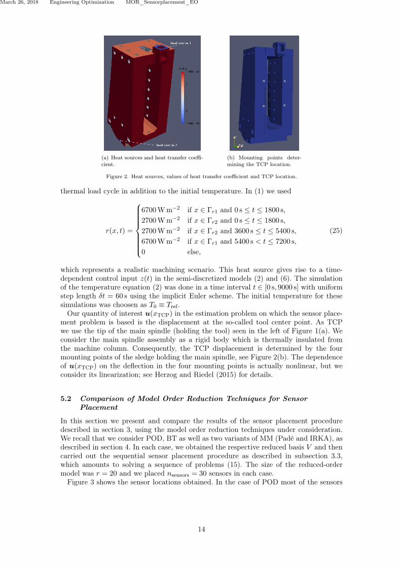
The following numerical experiments are based on the geometry of the prototypical Auer-bach ACW 630 machine column shown in Figure 1(b). The material constants are givenin Table 1. Notice that the heat transfer coefficient varies over different parts of theboundary, which are classified according to the orientation of the outer surface normal;see Figure 2(a). The machine column experiences the influence of two heat sources, seeagain Figure 2(a). One source originates from an electric drive mounted on the top of themachine column (surface part Γr1) while the other source represents the spindle drivingthe horizontal movement of the column (Γr2).The location of the heat sources enters the matrix Bth in (2) and (6) and thus it has an

impact on all reduced-order models. Note that the number of inputs is m = 3, becausethe ambient temperature Tref is considered as an input in order to achieve a linear (asopposed to affine) control system (2). For the generation of the snapshots needed forthe simulation based POD model order reduction technique we have to specify a typical

13


(a) Heat sources and heat transfer coeffi-cient.

(b) Mounting points deter-mining the TCP location.

Figure 2. Heat sources, values of heat transfer coefficient and TCP location.

thermal load cycle in addition to the initial temperature. In (1) we used

r(x, t) =

6700 W m−2 if x ∈ Γr1 and 0 s ≤ t ≤ 1800 s,

2700 W m−2 if x ∈ Γr2 and 0 s ≤ t ≤ 1800 s,

2700 W m−2 if x ∈ Γr2 and 3600 s ≤ t ≤ 5400 s,

6700 W m−2 if x ∈ Γr1 and 5400 s < t ≤ 7200 s,

0 else,

(25)

which represents a realistic machining scenario. This heat source gives rise to a time-dependent control input z(t) in the semi-discretized models (2) and (6). The simulationof the temperature equation (2) was done in a time interval t ∈ [0 s, 9000 s] with uniformstep length δt = 60 s using the implicit Euler scheme. The initial temperature for thesesimulations was choosen as T0 ≡ Tref.Our quantity of interest u(xTCP) in the estimation problem on which the sensor place-

ment problem is based is the displacement at the so-called tool center point. As TCPwe use the tip of the main spindle (holding the tool) seen in the left of Figure 1(a). Weconsider the main spindle assembly as a rigid body which is thermally insulated fromthe machine column. Consequently, the TCP displacement is determined by the fourmounting points of the sledge holding the main spindle, see Figure 2(b). The dependenceof u(xTCP) on the deflection in the four mounting points is actually nonlinear, but weconsider its linearization; see Herzog and Riedel (2015) for details.

5.2 Comparison of Model Order Reduction Techniques for SensorPlacement

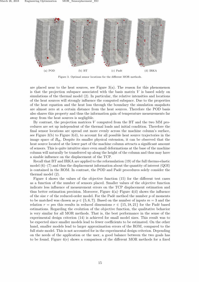
In this section we present and compare the results of the sensor placement proceduredescribed in section 3, using the model order reduction techniques under consideration.We recall that we consider POD, BT as well as two variants of MM (Padé and IRKA), asdescribed in section 4. In each case, we obtained the respective reduced basis V and thencarried out the sequential sensor placement procedure as described in subsection 3.3,which amounts to solving a sequence of problems (15). The size of the reduced-ordermodel was r = 20 and we placed nsensors = 30 sensors in each case.Figure 3 shows the sensor locations obtained. In the case of POD most of the sensors

14


(a) POD (b) BT (c) Padé (d) IRKA

Figure 3. Optimal sensor locations for the different MOR methods.

are placed near to the heat sources, see Figure 3(a). The reason for this phenomenonis that the projection subspace associated with the basis matrix V is based solely onsimulations of the thermal model (2). In particular, the relative intensities and locationsof the heat sources will strongly influence the computed subspace. Due to the propertiesof the heat equation and the heat loss through the boundary the simulation snapshotsare almost zero at a certain distance from the heat sources. Therefore the POD basisalso shares this property and thus the information gain of temperature measurements faraway from the heat sources is negligible.By contrast, the projection matrices V computed from the BT and the two MM pro-

cedures are set up independent of the thermal loads and initial condition. Therefore thefinal sensor locations are spread out more evenly across the machine column’s surface,see Figure 3(b) to Figure 3(d), to account for all possible heat source trajectories in theimage space of Bth. Despite its smaller physical extension, it can be observed that theheat source located at the lower part of the machine column attracts a significant amountof sensors. This is quite intuitive since even small deformations at the base of the machinecolumn will naturally be transferred up along the height of the column and thus may havea sizable influence on the displacement of the TCP.Recall that BT and IRKA are applied to the reformulation (19) of the full thermo-elastic

model (6)–(7) and thus the displacement information about the quantity of interest (QOI)is contained in the ROM. In contrast, the POD and Padé procedures solely consider thethermal model (2).Figure 4 shows the values of the objective function (15) for the different test cases

as a function of the number of sensors placed. Smaller values of the objective functionindicate less influence of measurement errors on the TCP displacement estimation andthus better estimation precision. Moreover, Figure 4(a)–Figure 4(d) shows the influenceof the size r of the reduced-order model. For the Padé method the number p of momentsto be matched was chosen as p ∈ 5, 6, 7. Based on the number of inputs m = 3 and therelation r = pm this results in reduced dimensions r ∈ 15, 18, 21 for the Padé basedestimations. Regarding the evolution of the objective function, the qualitative behavioris very similar for all MOR methods. That is, the best performance in the sense of theexperimental design criterion (14) is achieved for small model sizes. This result was tobe expected since smaller models lead to fewer coefficients to be estimated. On the otherhand, smaller models lead to larger approximation errors of the ROM, compared to thefull state model. This is not accounted for in the experimental design criterion. Dependingon the needs of the application or the user, a good balance between the two goals hasto be found. Figure 4(e) shows a comparison of the different MOR methods for a fixed

15


(a) POD (b) BT (c) Padé

(d) IRKA (e) Comparison for r = 20

Figure 4. Values of the optimal experimental design objective Ψ(Cov) for each MOR technique in dependence onthe ROM size r and the number of sensors placed.

(a) Estimated and simulated displacements at the TCPin mm.

(b) Relative errors.

Figure 5. Comparison of the exact (simulated by the full model) TCP displacement with the estimates (11) withsimulated measurements at the respective measurement locations (left) with heat sources (26). Relative errors areshown in the right plot.

dimension (r = 20) of the reduced systems. Here, the POD based approach shows bestperformance with respect to the optimization objective.Notice that the sequence of optimal sensor placement problems (15) operates under

the assumption that only temperature states in the range of the respective basis V canoccur. To achieve a more meaningful comparison of the four MOR variants we createdmeasurements from a simulation of the full model. The thermal loads in this simulationdiffer from those in (25), which were used to create the POD snapshots. The simulation

16


spans the time interval t ∈ [0 s, 7200 s] and we used the thermal loads

r(x, t) =

6700 W m−2 if x ∈ Γr1 and 0 s ≤ t ≤ 2400 s,

2700 W m−2 if x ∈ Γr2 and 0 s ≤ t ≤ 2400 s,

2700 W m−2 if x ∈ Γr2 and 2400 s ≤ t ≤ 4800 s,

6700 W m−2 if x ∈ Γr1 and 4800 s < t ≤ 7200 s,

0 else

(26)

and an initial temperature of T0 ≡ Tref. Figure 5(a) and Figure 5(b) show the evolution ofthe simulated TCP deflection, compared to its estimated position based on the nsensors =30 optimally placed sensors (in the sense of the approach in subsection 3.3) with reducedbases of dimension r = 20. For each reduced order model the simulated temperaturevalues were evaluated at the relevant sensor locations. The TCP displacement estimatewas then obtained from solving the least-squares problem (11).Again, according to the relative errors between simulated and estimated TCP displace-

ments, the POD approach yields the best results in this exercise. The estimation of theTCP displacement associated to the subspace spanned by the Padé procedure shows sig-nificant inaccuracies at times t = 120 s and t = 4800 s. This may be due to the factthat the matching of p = 7 moments of the transfer function at a single expansion points0 = 0 and a resulting reduced dimension r = 21, restricted to r = 20, cannot sufficientlyapproximate the actual model behavior of the original full-order model at those points.Apart from these peaks, the BT, Padé and IRKA based estimates are roughly of thesame order of accuracy. Note that the large relative errors at the beginning of the timeinterval are mainly caused by the fact that the trajectories evolve closely around zero andtherefore the relative error is violated by divisions of values that are close to zero. How-ever, it is a well known fact that the reduced-order models based on POD are in generalonly reliable for operating conditions near those used to generate the POD snapshots.We therefore repeat the experiment with thermal loads

rmod(x, t) =

3000 W m−2 if x ∈ Γr1 and 0 s ≤ t ≤ 2400 s,

5000 W m−2 if x ∈ Γr2 and 0 s ≤ t ≤ 2400 s,

5000 W m−2 if x ∈ Γr2 and 2400 s ≤ t ≤ 4800 s,

3000 W m−2 if x ∈ Γr1 and 4800 s < t ≤ 7200 s,

0 else,

(27)

which differ more significantly from the nominal loads (25) than (26). Figure 6(a) andFigure 6(b) show the estimation quality in this case. Here, we observe that the change ofthe intensity of the heat sources does not considerably influence the estimations comparedto the previous scenario. Only the POD approach performs slightly worse and producesnow similar errors than the other MOR methods.In a final experiment the robustness of the TCP displacement estimation with respect

to noisy measurements using a standard deviation of σ = 0.1 is analyzed in Figure 7(a)and Figure 7(b). The heat sources were chosen as in (26). The TCP evolution trajectoriesand the corresponding relative errors, again, reveal the superiority of the POD approachapplied to the optimal experimental design framework, while the other strategies are ofthe same order of accuracy as before.

17




Figure 6. Same as Figure 5 using alternative heat sources (27).



Figure 7. Same as Figure 5 with heat sources (26) using noisy measurements.

5.3 Discussion

In this paper we revisited an optimal sequential placement strategy for temperaturesensors in order to predict thermally induced mechanical deformations from temperaturemeasurements. To make the sensor placement procedure tractable, we applied modelorder reduction either to the temperature equation alone, or to the full thermo-mechanicalmodel. The main focus of this paper was to compare the performance of different MORmethods w.r.t. the sensor placement objective and the prediction quality of the induceddisplacement estimation using simulated measurements at the optimized sensor positions.

18


Comparing the simulation results being based on the data used as the POD trainingscenario and a fixed model size of r = 20, the POD approach showed the best performancew.r.t. the experimental design objective as well as the estimation accuracy of the TCPdisplacement. Considering thermal loads apart from the POD training set, as well as fornoisy measurement data, the POD, BT, and IRKA based MOR approaches basically showthe same behavior w.r.t. the estimation accuracy. POD, as a simulation based MOR ap-proach, depends on the snapshot ensemble to be sufficiently rich to yield a reliable ROM.Nevertheless, we found POD to work well even under significant perturbations of theheating profile used during the training phase, compared to the other MOR schemes. In-terestingly, POD shows best performance w.r.t. to the prescribed reduced order/numberof sensors and the comparison criteria even though it targets only the temperature fieldand no information about the true QOI (the TCP displacement in our case) is included.POD especially takes into account the explicit influence of the actual acting loads and,according to that, clusters the sensors corresponding to the regions of dominant thermalinterest.The three other MOR methods which were considered do not depend on simulations.

Moreover, the BT and IRKA approaches operate on an equivalent reformulation of thefull thermo-mechanical model and thus include QOI information. On the other hand,these methods do not consider the actual machining process. Therefore, they are lessspecialized such that the corresponding ROMs need to be significantly larger in orderto achieve comparable performance. Still, for drastically changed machining processes,e.g. with no action on the lower heat source, they are expected to give much betterresults than the POD without modification, i.e., regeneration of the POD basis by newtraining with the changed input situation. However, quantification of the degenerationof the POD model requires further investigation. Out of these methods, the BT and theIRKA moment matching approaches performed best, and very similarly.

Acknowledgment

This work was supported by two DFG grants within the Special Research Program SFB/Transregio 96 (Thermo-energetische Gestaltung von Werkzeugmaschinen), which is grate-fully acknowledged.

References

Alonso, A.A., C.E. Frouzakis, and I.G. Kevrikidis. 2004. “Optimal sensor placement for statereconstruction of distributed process systems.” AIChE Journal 50 (7): 1438–1452.

Alonso, A.A., I.G. Kevrekidis, J.R. Banga, and C.E. Frouzakis. 2004. “Optimal sensor locationand reduced order observer design for distributed process systems.” Computers & ChemicalEngineering 28 (1-2): 27–35.

Antoulas, A.C. 2005. Approximation of large-scale dynamical systems. Vol. 6 of Advances inDesign and Control. Philadelphia, PA: Society for Industrial and Applied Mathematics (SIAM).With a foreword by Jan C. Willems.

Armaou, A., and M.A. Demetriou. 2006. “Optimal actuator/sensor placement for linear parabolicPDEs using spatial norm.” Chemical Engineering Science 61 (22): 7351–7367.

Benner, P., P. Kürschner, and J. Saak. 2013a. “An improved numerical method for balancedtruncation for symmetric second-order systems.” Mathematical and Computer Modelling ofDynamical Systems 19 (6): 593–615.

Benner, P., P. Kürschner, and J. Saak. 2013b. “A Reformulated Low-Rank ADI Iteration withExplicit Residual Factors.” Proceedings in Applied Mathematics and Mechanics 13 (1): 585–586.

Benner, P., P. Kürschner, and J. Saak. 2014/15. “Self-generating and efficient shift parameters

19

http://transregio96.de

http://transregio96.de


in ADI methods for large Lyapunov and Sylvester equations.” Electronic Transactions onNumerical Analysis 43: 142–162.

Benner, P., and A. Schneider. 2013. Balanced Truncation for Descriptor Systems with ManyTerminals. Preprint MPIMD/13-17. Max Planck Institute Magdeburg.

Boley, B.A., and J.H. Weiner. 1960. Theory of thermal stresses. New York London: John Wiley& Sons Inc.

Braess, D. 2007. Finite Elements: Theory, Fast Solvers, and Applications in Solid Mechanics.Cambridge: Cambridge University Press.

Cohen, K., S. Siegel, and T. McLaughlin. 2006. “A heuristic approach to effective sensor placementfor modeling of a cylinder wake.” Computers & Fluids 35 (1): 103–120.

Enns, D.F. 1984. “Model reduction with balanced realizations: An error bound and a frequencyweighted generalization.” In The 23rd IEEE Conference on Decision and Control, 127–132.Dec.

Eslami, M.R., R.B. Hetnarski, J. Ignaczak, N. Noda, N. Sumi, and Y. Tanigawa. 2013. Theoryof elasticity and thermal stresses. Vol. 197 of Solid Mechanics and its Applications. Dordrecht:Springer. Explanations, problems and solutions.

Fedorov, V.V., and P. Hackl. 1997. Model-oriented design of experiments. Vol. 125 of LectureNotes in Statistics. New York: Springer-Verlag.

García, M.R., C. Vilas, J.R. Banga, and A.A. Alonso. 2007. “Optimal Field Reconstruction ofDistributed Process Systems from Partial Measurements.” Industrial & Engineering ChemistryResearch 46 (2): 530–539.

Glover, K. 1984. “All optimal Hankel-norm approximations of linear multivariable systems andtheir L∞-error bounds.” International Journal of Control 39 (6): 1115–1193.

Green, K. 2006. “Optimal Sensor Placement for Parameter Identification.” Master thesis. RiceUniversity, Houston.

Grossmann, C., H.-G. Roos, and M. Stynes. 2007. Numerical Treatment of Partial DifferentialEquations. Universitext. Berlin: Springer. Translation and Revision of the 3rd edition of "Nu-merische Behandlung partieller Differentialgleichungen" published by Teubner, 2005.

Gugercin, S., A.C. Antoulas, and C. Beattie. 2008. “H2 model reduction for large-scale lineardynamical systems.” SIAM Journal on Matrix Analysis and Applications 30 (2): 609–638.

Herzog, R., and I. Riedel. 2015. “Sequentially Optimal Sensor Placement in Thermoelastic Modelsfor Real Time Applications.” Optimization and Engineering 16 (4): 737–766.

Kammer, D.C. 1991. “Sensor placement for on-orbit modal identification and correlation of largespace structures.” Journal of Guidance, Control, and Dynamics 14 (2): 251–259.

Koevoets, A. H., H. J. Eggink, J. Van der Sanden, J. Dekkers, and T. A M Ruijl. 2007. “Op-timal sensor configuring techniques for the compensation of thermo-elastic deformations inhigh-precision systems.” In 13th International Workshop on Thermal Investigation of ICs andSystems, 2007, 208–213.

Körkel, S., H. Arellano-Garcia, J. Schöneberger, and G. Wozny. 2008. “Optimum experimental de-sign for key performance indicators.” In Proceedings of 18th European Symposium on ComputerAided Process Engineering, Vol. 25575–580.

Kunisch, K., and S. Volkwein. 2001. “Galerkin proper orthogonal decomposition methods forparabolic problems.” Numerische Mathematik 90 (1): 117–148.

Kürschner, P. 2016. “Efficient Low-Rank Solution of Large-Scale Matrix Equations.” Dissertation.Otto-von-Guericke-Universität Magdeburg.

Laub, A., M. Heath, C. Paige, and R. Ward. 1987. “Computation of system balancing transforma-tions and other applications of simultaneous diagonalization algorithms.” IEEE Transactionson Automatic Control 32 (2): 115–122.

Meo, M., and G. Zumpano. 2005. “On the optimal sensor placement techniques for a bridgestructure.” Engineering Structures 27 (10): 1488–1497.

Mokhasi, P., and D. Rempfer. 2004. “Optimized sensor placement for urban flow measurement.”Physics of Fluids 16 (5): 1758–1764.

Moore, B. 1981. “Principal component analysis in linear systems: Controllability, observability,and model reduction.” IEEE Transactions on Automatic Control 26 (1): 17–32.

Saad, Y. 2003. Iterative Methods for Sparse Linear Systems. 2nd ed. Philadelphia: Society forIndustrial and Applied Mathematics (SIAM).

20


Seber, G.A.F., and C.J. Wild. 2005. Nonlinear Regression. Wiley Series in Probability and Statis-tics. John Wiley & Sons.

Sun, H., and O Büyüköztürk. 2015. “Optimal sensor placement in structural health monitoringusing discrete optimization.” Smart Materials and Structures 24 (12): 125034.

Uciński, D. 2005. Optimal measurement methods for distributed parameter system identification.Systems and Control Series. Boca Raton, FL: CRC Press.

Uciński, D., and M. Patan. 2007. “D-optimal design of a monitoring network for parameter esti-mation of distributed systems.” Journal of Global Optimization 39 (2): 291–322.

Willcox, K. 2006. “Unsteady flow sensing and estimation via the gappy proper orthogonal decom-position.” Computers & Fluids 35 (2): 208–226.

Yi, T.-H., H.-N. Li, and M. Gu. 2011. “Optimal sensor placement for structural health monitoringbased on multiple optimization strategies.” The Structural Design of Tall and Special Buildings20 (7): 881–900.

Yildirim, B., C. Chryssostomidis, and G.E. Karniadakis. 2009. “Efficient sensor placement forocean measurements using low-dimensional concepts.” Ocean Modelling 27 (3–4): 160–173.

21

Date post:	08-Jun-2018
Category:	Documents
Upload:	hahanh
View:	215 times
Download:	0 times

Comparison of Model Order Reduction Methods for …2018 EngineeringOptimization...

Documents