1 SANDIA REPORT SAND2013-8847 Unlimited Release Printed October 2013 Comparison of Open-Source Linear Programming Solvers Jared L. Gearhart, Kristin L. Adair, Richard J. Detry, Justin D. Durfee, Katherine A. Jones, Nathaniel Martin Prepared by Sandia National Laboratories Albuquerque, New Mexico 87185 and Livermore, California 94550 Sandia National Laboratories is a multi-program laboratory managed and operated by Sandia Corporation, a wholly owned subsidiary of Lockheed Martin Corporation, for the U.S. Department of Energy's National Nuclear Security Administration under contract DE-AC04-94AL85000. Approved for public release; further dissemination unlimited.
Transcript
1
SANDIA REPORT SAND2013-8847 Unlimited Release Printed October 2013
Comparison of Open-Source Linear Programming Solvers Jared L. Gearhart, Kristin L. Adair, Richard J. Detry, Justin D. Durfee, Katherine A. Jones, Nathaniel Martin Prepared by Sandia National Laboratories Albuquerque, New Mexico 87185 and Livermore, California 94550
Sandia National Laboratories is a multi-program laboratory managed and operated by Sandia Corporation, a wholly owned subsidiary of Lockheed Martin Corporation, for the U.S. Department of Energy's National Nuclear Security Administration under contract DE-AC04-94AL85000. Approved for public release; further dissemination unlimited.
2
Issued by Sandia National Laboratories, operated for the United States Department of Energy by Sandia Corporation. NOTICE: This report was prepared as an account of work sponsored by an agency of the United States Government. Neither the United States Government, nor any agency thereof, nor any of their employees, nor any of their contractors, subcontractors, or their employees, make any warranty, express or implied, or assume any legal liability or responsibility for the accuracy, completeness, or usefulness of any information, apparatus, product, or process disclosed, or represent that its use would not infringe privately owned rights. Reference herein to any specific commercial product, process, or service by trade name, trademark, manufacturer, or otherwise, does not necessarily constitute or imply its endorsement, recommendation, or favoring by the United States Government, any agency thereof, or any of their contractors or subcontractors. The views and opinions expressed herein do not necessarily state or reflect those of the United States Government, any agency thereof, or any of their contractors. Printed in the United States of America. This report has been reproduced directly from the best available copy. Available to DOE and DOE contractors from U.S. Department of Energy Office of Scientific and Technical Information P.O. Box 62 Oak Ridge, TN 37831 Telephone: (865) 576-8401 Facsimile: (865) 576-5728 E-Mail: [email protected] Online ordering: http://www.osti.gov/bridge Available to the public from U.S. Department of Commerce National Technical Information Service 5285 Port Royal Rd. Springfield, VA 22161 Telephone: (800) 553-6847 Facsimile: (703) 605-6900 E-Mail: [email protected] Online order: http://www.ntis.gov/help/ordermethods.asp?loc=7-4-0#online
3
SAND2013-8847 Unlimited Release
Printed October 2013
Comparison of Open-Source Linear Programming Solvers
Jared L. Gearhart, Kristin L. Adair, Justin D. Durfee, Katherine A. Jones, Nathaniel Martin
Operations Research and Computational Analysis Sandia National Laboratories
P.O. Box 5800 Albuquerque, New Mexico 87185-MS1188
Richard J. Detry
ISR Real Time Processing Sandia National Laboratories
P.O. Box 5800 Albuquerque, New Mexico 87185-MS0532
Abstract
When developing linear programming models, issues such as budget limitations, customer requirements, or licensing may preclude the use of commercial linear programming solvers. In such cases, one option is to use an open-source linear programming solver. A survey of linear programming tools was conducted to identify potential open-source solvers. From this survey, four open-source solvers were tested using a collection of linear programming test problems and the results were compared to IBM ILOG CPLEX Optimizer (CPLEX) [1], an industry standard. The solvers considered were: COIN-OR Linear Programming (CLP) [2], [3], GNU Linear Programming Kit (GLPK) [4], lp_solve [5] and Modular In-core Nonlinear Optimization System (MINOS) [6]. As no open-source solver outperforms CPLEX, this study demonstrates the power of commercial linear programming software. CLP was found to be the top performing open-source solver considered in terms of capability and speed. GLPK also performed well but cannot match the speed of CLP or CPLEX. lp_solve and MINOS were considerably slower and encountered issues when solving several test problems.
4
ACKNOWLEDGMENTS This work was funded by the Office of the Under Secretary of Defense for Acquisition, Technology, & Logistics (AT&L).
Appendic C: List of Test Problems ............................................................................................... 45
Appendix D: Test Problem Read Errors ....................................................................................... 51
Appendix E: Comparison of CLP 1.7.4 and 1.14 ......................................................................... 53
FIGURES Figure 1. Plot of Problem Size in Terms of Constraints and Variables ........................................ 19 Figure 2. Plot of Solution Times versus the Number of Constraints for each Solver ................... 29 Figure 3. Plot of Solution Times versus the Number of Variables ............................................... 29 Figure 4. Plot of Solution Times versus the Number of Non-zero Elements ............................... 30
TABLES Table 1. Candidate LP Solvers Identified During First Round Screening ................................... 12 Table 2. List of Modeling Environments Identified During the Initial Screening Process ......... 12
6
Table 3. List of Integer and Quadratic Program Solvers Identified During the Initial Screening Process .......................................................................................................................................... 13 Table 4. Summary of LP Solvers Eliminated During Second Round of Testing ......................... 14 Table 5. Summary of Key Aspects of Tested Solvers .................................................................. 14 Table 6. Number of Test Problems in Each Problem Set ............................................................. 19 Table 7. Comparison of Solution Times for CLP Interior Point and Simplex Algorithms .......... 22 Table 8. Comparison of Solution Times for GLPK Interior Point and Simplex Algorithms ....... 24 Table 9. Summary of Simplex Solution Results for Each Solver ................................................. 26 Table 10. Comparison of “Easy” Problem Solution Times for Each Solver ................................ 28 Table 11. Comparison of Geometric Means (in Seconds) of “Easy” Problem Solution Times for Each Solver ................................................................................................................................... 28 Table 12. CLP and CPLEX Solution Times for “Hard” Problems. Italics indicate problems that timed out. Bold indicates the fasted solver (CLP or CPLEX). ..................................................... 31 Table 13. First Round Screening Results for Tools Listed in INFORMS LP Software Survey [7]....................................................................................................................................................... 39 Table 14. First Round Screening Results of Propriety LP Tool from Wikipedia [8] ................... 40 Table 15. First Round Screening Results of Non-propriety LP Tool from Wikipedia [8] ........... 41 Table 16. First Round Screening Results from a General Survey of LP Websites ...................... 42 Table 17. List of Top Open-Source LP Modeling Environments. Solvers studied in this model are highlighted in bold. Other open-source solvers are italicized. ................................................ 43 Table 18. Listing of Test LP Problems ......................................................................................... 50 Table 19. Comparison of Total Solution Times (Seconds) for Each “Easy” Problem Set Using the Dual Simplex Algorithms for CLP 1.7.4 and CLP 1.14 ......................................................... 54 Table 20. Comparison of Total Solution Times (Seconds) for Each “Easy” Problem Set Using the Primal Simplex Algorithms for CLP 1.7.4 and CLP 1.14 ...................................................... 55 Table 21. Comparison of Total Solution Times (Seconds) for Each “Easy” Problem Set Using CPLEX, CLP 1.7.4, and CLP 1.14 ............................................................................................... 56 Table 22. Various Statistics Comparing CPLEX, CLP 1.7.4, and CLP 1.14 for the “Hard” Test Problems ....................................................................................................................................... 58
7
NOMENCLATURE API Application Programming Interface CCO Contingency Contractor Optimization CLP COIN-OR Linear Programming COIN Computational Infrastructure for Operations Research COIN-OR See COIN DoD Department of Defense GLPK GNU Linear Programming Kit GMPL GNU Mathematical Programming Language IP Integer Programming LP Linear Programming MINOS Modular In-core Nonlinear Optimization System OPL Optimization Programming Language
8
9
1. INTRODUCTION This report documents a study that was conducted as part of the Contingency Contractor Optimization (CCO) project to determine if there are viable open-source linear programming (LP) solvers that could be used in place of commercial LP solvers. One requirement of the CCO project is that all software and algorithms developed or used by the final engineering prototype should be freely distributable within the Department of Defense (DoD). Since the core model developed for this project was an LP, it was necessary to create or identify a low-cost or no-cost solver. Production licenses for standard commercial LP solvers such as CPLEX [1] have annual costs of tens of thousands of dollars, which precluded their use for the CCO project. In order to fulfill the freely distributable requirement, a survey and assessment of alternative LP solvers was conducted. While this study was motivated by the CCO project, the findings are general and should be useful to any group who is interested in using a low-cost or no-cost LP solver. This study was divided into two phases. In the first phase, a survey was conducted of all available LP tools to identify which ones could be used given the requirements of the CCO project. In the second phase, the most promising LP solvers identified during the survey were tested on a range of problems to determine the quality of each solver. Since the solver selected for the CCO project will be used in a production environment, it is important that the solver be accurate, efficient, and mature. Therefore, each solver was also compared to IBM’s CPLEX solver, an industry standard. This report is organized as follows: Section 2 discusses the findings from the survey of the LP solvers. Section 3 describes the testing approach and results used for a subset of the available solvers. Section 4 provides a summary and conclusion.
10
11
2. SURVEY AND SELECTION OF LP SOLVERS This section describes the results of a survey of available LP solver tools. This survey was conducted in two rounds. The first round focused on reviewing all of the available tools and eliminating those which were not LP solvers and would not meet the requirements of the CCO project (free or low-cost, usable in a production environment for a government application, and not tied to a commercial product such as MATLAB). Once this initial survey was completed and candidate solvers were identified, a second round screening was conducted to identify the top LP solvers that would be tested. 2.1 Initial Screening: Survey of LP Tools An initial screening of LP tools was conducted using two types of data sources. The first data source was a survey of linear programming software conducted by Robert Fourer [7], available through the INFORMS website. The second source of data was a general web search for linear programming tools. Modeling-related websites provided lists of both commercial and free LP solvers [8], [9], [10]. Once this survey was complete, each product was reviewed and screened according to the following criteria with the desired answer of “Yes”:
- Is the product free or low-cost? - Is the product an LP solver? - Does the product use an exact method such as the Simplex algorithm or an Interior Point
algorithm?; (tools using heuristic methods such as Monte Carlo sampling or genetic algorithms are discounted, since there are well established exact algorithms for solving LPs)
- Is the product mature?; (as demonstrated through software development practices, documentation, and active commercial or academic user communities)
- Is the product a stand-alone product (e.g. not an add-in to MATLAB, Excel)? In total, about 100 LP tools were identified using the two data sources described above. The screening criteria above were then applied to this list to create a down-selected list of solvers. A complete list of all the tools considered and the justification for why they were accepted or rejected in the first round of screening can be found in Appendix A. The initial screening identified ten potential LP solvers. These solvers are listed in Table 1.
12
Solver Name Website lp_solve http://lpsolve.sourceforge.net/5.5/ MINOS http://www.sbsi-sol-
Table 1. Candidate LP Solvers Identified During First Round Screening
In addition to LP solvers, the screening process identified several other sets of tools that might be of potential use to those requiring open-source math programming tools. These tools are summarized in Table 2 and Table 3. Table 2 lists the modeling environments that were identified during the survey. In general, it is very difficult to develop models by interacting directly with solvers. A commonly used approach is to create problem statements in a modeling environment and then pass the problem to a solver. Table 3 lists quadratic program and integer program solvers that were identified during the survey. While not directly applicable to this study, it is worth pointing out that open-source tools also exist for integer and quadratic programming. CLP and PPL are included in both Table 1 and Table 3, since they are both linear and quadratic programming solvers.
Software Name Website Coopr https://software.sandia.gov/trac/coopr CMPL https://projects.coin-or.org/Cmpl OptimJ http://www.ateji.com/optimj/index.html PuLP http://code.google.com/p/pulp-or/ OpenOpt http://openopt.org/Welcome Microsoft Solver Foundation
Table 3. List of Integer and Quadratic Program Solvers Identified During the Initial Screening Process 2.2 Second Screening: Down-Selection of LP Solvers Given time and resource limitations, only four of the solvers identified during the initial screening could be tested. A second round of screening was conducted to identify the top four candidates for testing. All of the same selection criteria were applied during the second round as the first. However, during the second round, the solvers were scrutinized more closely and compared against each other. The second round of screening identified lp_solve, MINOS, CLP, and GLPK as the test candidates. A complete description of each of these tools is provided in section 2.3; however they do have common desirable traits. First, all of the tested solvers have a mature code base and are extensively documented. MINOS is a commercial solver that can be purchased with AMPL and GAMS [9], [10]. While it is not free, it was included since it is available to the government for $350 [11]. The other three solvers are open-source applications. In a survey of websites, presentations, and papers discussing open-source solvers ( [7], [8], [9], [10], [12], [13], [14], [15]), these three solvers were referenced the most often. Also, all of the major open-source development environments provide an interface to some combination of these three tools (see Appendix B). The six tools that were eliminated during the second screening and the reason they were eliminated are given below in Table 4. 2.3 Discussion of Selected Solvers The solvers selected for further testing based on the results from the second screening were: CLP, GLPK, lp_solve and MINOS. A discussion of each of these solvers is provided in the following sub-sections. Table 5 provides a summary of the key aspects of each solver described in the sub-sections below.
14
LP Solver Reason Rejected PCx PCx has not been updated since 2006. This was rejected since other
solvers that are in active development were available. PPL The PPL code is mature and has good software development practices
and documentation. However, it is not widely used. It is not referenced in any of the sources used in the screening process nor do any of the researched modeling environments provide accesses to this tool.
JOptimizer JOptimizer is a relatively new project and is not widely used at this time. It is not referenced in any of the sources used in the screening process nor do any modeling environments provide access to the tool.
LiPS LiPS was developed to teach linear programming in an academic setting and is not intended to be used in production. It is not referenced in any of the sources used in the screening process nor do any modeling environments provide access to the tool.
CVXOPT The CVXOPT code contains many useful algorithms, but it was developed for use in a research environment and is not intended to be used in production. It is not referenced in any of the sources used in the screening process nor do any modeling environments provide access to the tool.
QSOPT The QSOPT code contains many useful algorithms, but it was developed by a university and intended for research uses. Apart from being tested by Hans Mittleman [15], it is not referenced in any of the other sources used in the screening process nor do any modeling environments provide access to the tool.
Table 4. Summary of LP Solvers Eliminated During Second Round of Testing
LP Solver Command
Line Interface?
Application Programming Interface (API)
Input File Algorithms
CLP Y C++ MPS, Free MPS Primal and Dual Simplex, Interior Point
GLPK Y C, Java MPS, Free MPS, LP, GLPK, MathProg
Primal and Dual Simplex, Interior Point
lp_solve Y Java, .NET, C, C++, C#
MPS, Free MPS, LP Primal and Dual Simplex
MINOS Y Fortran, C, MATLAB
MPS, LP + SPEC File Primal Simplex
Table 5. Summary of Key Aspects of Tested Solvers
15
2.3.1 COIN-OR Linear Programming (CLP) COIN-OR Linear Programming (CLP) is a project that is part of the Computational Infrastructure for Operations Research (COIN-OR, or simply COIN) initiative [2], [16]. COIN-OR is an initiative to encourage development of open-source, operations research software. CLP is an LP solver containing Dual and Primal Simplex algorithms. It has been tested on problems of up to 1.5 million constraints and is as reliable as OSL [17]. CLP is available under the Eclipse Public License version 1.0. CLP has also been tested by Hans Mittelmann [15] and was mentioned in several references discussing LP solvers [13], [14]. CLP is written in the C++ programming language. Its primary algorithms are the Primal and Dual Simplex algorithms, but it also contains an Interior Point algorithm. Users can interact with CLP through an interactive command line or through a C++ application programming interface (API). While the user can create LP problem statements in code through the API, CLP is also able to accept MPS, Free MPS and LP files [2]. These three file formats are standards for specifying LP problems. All LP solvers are capable of reading one of more of these formats. 2.3.2 GNU Linear Programming Kit (GLPK) GNU Linear Programming Kit (GLPK) is a math programming project that is part of the GNU project [4]. It was developed to solve large scale LP problems. GLPK was developed by Andrew Makhorin of the Moscow Aviation Institute. GLPK is available under the GNU General Public License. It can solve LPs using Primal and Dual Simplex algorithms, as well as an Interior Point algorithm. Like CLP, it has been tested by Hans Mittelmann [15] and was referenced in several sources pertaining to LP solvers [13] , [14]. GLPK is written in the C programming language. Users can interact with GLPK through the command line or through an API. GLPK offers a C and Java API. GLPK accepts models in the MPS, Free MPS and LP format. It also accepts problem statements in the MathProg format which are created using the GNU Mathematical Programming Language (GMPL), a modeling environment related to GLPK. 2.3.3 lp_solve lp_solve [5] is an LP and integer programming (IP) solver based on the revised Simplex Method and the branch-and-bound method for the integers. It is freely available under the GNU Lesser General Public License. It was originally developed by Michel Merelaar at Eindhoven University of Technology but has had many contributors since the original development. It uses the Primal and Dual Simplex algorithms for solving LP models. lp_solve is an active project and is referenced in several sources [13], [14]. lp_solve is written in the C programming language. Users can interact with lp_solve through the command line of through an API. lp_solve offers a C, C#, C++, Java, and .NET API. lp_solve can read the MPS, Free MPS and LP file format.
16
2.3.4 MINOS MINOS [6] is a commercial software package sold by Stanford Business Software, Inc. MINOS stands for Modular In-core Nonlinear Optimization System. It was developed by Stanford University and was supported by a grant from the U.S. government. It is able to solve both non-linear and linear programs. Development on MINOS is not as active as the other three solvers selected for testing. Version 5.0 was released in 1983, and the most recent version (5.51) was released in 2002. Also, MINOS was not referenced in any of the sources used in this effort discussing LP solvers. However, MINOS is used by commercial modeling languages such as AMPL [9] and GAMS [10]. Since the development of MINOS was funded by the U.S. government, a government organization can purchase a license at a cost of $350, which can be used indefinitely by the entire organization at a single site. Since MINOS offers a low-cost commercial option for government use, it was selected for testing despite the fact that it is not actively being developed. MINOS is written in the Fortran 77 programming language and distributed as source code. Users can interact with MINOS through the command line or an API. MINOS offers Fortran, C, and MATLAB APIs. Unlike the other solvers, MINOS is only able to support the MPS file format. MINOS also requires that a SPEC or specification file be created by the user which specifies problem specific parameters related to MPS, in addition to settings for the solver. This is different from the other solvers, which are able to determine the problem specific parameters by reading the MPS file. This means that the user must create both a MPS and SPEC file before using MINOS.
17
3. LP SOLVER TESTING Each of the solvers selected during the screening process were tested using a collection of LP test problems drawn from several sources. These results were compared to IBM’s CPLEX solver. The testing focused on addressing two important questions for each solver. First, is the solver able to solve each problem to optimality? Second, how long does it take each solver to solve each problem? Before these questions could be addressed, a collection of test LP problems was created. Section 3.1 describes the test problems used for this study. Section 3.2 describes the results when each solver was tested using the test problems. 3.1 Test LP Problems In order to test each solver, a collection of test problems was created. While the motivation behind this effort was to find a solver for the CCO problem, a much broader test data set was created. The need for a free and freely distributable solver was identified during the second phase of the CCO project. The goal of the third phase of this effort is to create an engineering prototype based on an electronic storyboard prototype created during Phase 2. During Phase 2, a collection of demonstration data sets were created. Since the CCO tool is still in development, the size of problems when real data is used is not yet well-defined. Given this, a more holistic testing approach was taken, where the test problems ranged from very small problems to problems several orders of magnitude larger than the CCO demonstration problems developed during Phase 2. By using this approach, confidence could be gained that the selected solver would be able to solve larger problems in the future should the data change. A total of 201 test problems were identified using three data sources. The first data source was Netlib [18] which is a repository that contains collections of test data sets which can be used for benchmarking various algorithms. Specifically, the LP library was used. The LP problems in Netlib are divided into three groups: the main data set (referred to here as just Netlib), Infeasible, and Kennington. A total of 138 problems were drawn from these problem sets. Netlib contains a total of 97 problems, 93 of which were used during the testing. The remaining four test problems required a conversion process to generate an MPS file, and were excluded from the test set. These problems are generally small, with most constraints (row) counts in the hundreds to low thousands and most variables (column) counts in the hundreds to ten thousand range. The largest number of constraints and variables was 6,071 and 13,525 respectively. The Infeasible problem set contains 29 infeasible problems, all of which were included in the set of test problems. These problems are generally the same size as the Netlib problems, with a maximum of 3,792 constraints and 10,733 variables. Finally, the Kennington data set contains 16 problems, all of which were included in the set of test problems. These problems are slightly larger than the Netlib and Infeasible problems, with row and column counts ranging from the thousands to low hundreds of thousands. The maximum constraints and variables counts were 105,127 and 232,966, respectively. The second data source was the pre-loaded examples included with the CCO prototype developed during Phase 2. Twelve model runs were selected for testing. This problem set was included since the intention of this study was to determine a replacement solver that could solve CCO problems. These problems were created by using the Optimization Programming Language
18
(OPL)/CPLEX implementation of the CCO model from Phase 2. A CPLEX setting was used to export each problem to a Free MPS file. The problems created through this approach were very large, with constraint counts ranging from 47,522 to 181,443 and variable counts ranging from 517,971 to 2,106,004. Further investigation into the Phase 2 implementation of the CCO model revealed that it created problems which were much larger than necessary, and that the size of the problem could be reduced by eliminating unnecessary constraints and variables. This was not a concern during Phase 2, since CPLEX was able to quickly pre-solve the model, eliminating the excess constraints and variables. In order to provide a more fair comparison between the solvers, 12 simplified problems were created by pre-solving each of the original 12 problems. This was accomplished using CLP’s pre-solve option and writing a new MPS file (the solutions to both the original and modified problems were compared to ensure they were the same). The resulting problems are considerably smaller with constraint counts between 1,608 and 2,889, and variable counts between 2,954 and 5,414. In total, 24 CCO problems are tested: 12 “Large CCO” problems and 12 “Small CCO” problems. The final data source was a set of test problems made available by Professor Hans Mittelman from Arizona State University [15]. A total of 39 were selected from this source. These problems were divided into six categories based on the folders containing the files on the website: Plato, FOME, Misc, Nug, PDS, and Rail. These problems were selected because they are large and tend to be difficult to solve. The size of these problems ranges from tens of thousands to around one million constraints and variables. The maximum numbers of constraints and variables are 1,918,399 and 1,259,121, respectively. For testing purposes, the 201 test problems were divided into two groups: “easy” and “hard” problems. An initial screening of the test problems using CPLEX revealed that some of the problems in the Plato, Misc, and Nug problems sets were especially difficult to solve. The 21 problems in these data sets were categorized as “hard” problems and excluded from the initial testing. The remaining 180 “easy” problems were used for the first round of testing. It should be noted that the terms “easy” and “hard” are only designated with respect to CPLEX solve time. As the results section will show, some of the “hard” problems were solved very quickly with other LP solvers while other solvers took a very long time on the same problems. Conversely, while CPLEX was able to solve the “easy” problems in seven minutes, some other solvers were unable to obtain an optimal solution to all of these problems after several days. Figure 1 shows the size of each test problem in terms of the number of constraints and variables. The problems are grouped into the “hard” and “easy” data sets. Observe that while there is some overlap between these two sets, the “hard” problems tend to be larger than most of the “easy” problems. Also note that this collection of test problems covers a wide range of problem sizes (the arrows indicate the largest problems in each set). Table 6 shows the number of test problems in each set. Appendix C contains a complete listing of the test problems.
19
Figure 1. Plot of Problem Size in Terms of Constraints and Variables
Problem Set Number of
Problems Netlib 93 Infeasible 29 Kennington 16 Large CCO 12 Small CCO 12 Plato 2 PDS 8 Rail 5 FOME 5 Misc 16 Nug 3 Grand Total 201
Table 6. Number of Test Problems in Each Problem Set
3.2 LP Solver Tests The following sub-sections describe the various tests that were conducted for each LP solver. The general approach was to test all four candidate solvers using the 180 “easy” problems. Based on the results from this initial test, the best solver would also be tested using the 21 “hard” problems. All of the problem statements were passed to the model through the command line
Number of Constraints and Variables for each Test Problem
"Easy" MPS
"Hard" MPS
181,443 Constraints &2,106,004 Variables
1,259,121 Variables
1,918,399 Constraints
20
interface in the MPS or Free MPS format. Each solver was given four hours to solve each “easy” problem and eight hours to solve each “hard” problem. The primary algorithms of interest for each solver were the Primal and Dual Simplex algorithms (as applicable). For each solver, both algorithms were run for each problem and the best solution time was used. This was motivated by the fact that certain problems may be easier to solve using one of these algorithms. Additionally, the Interior Point algorithms for CLP and GLPK were tested to see if they offered any benefits over the associated Simplex algorithms. Unless otherwise stated, all of the results associated with the time required to read or solve a problem are based on rounding the actual time to the nearest tenth of a second, since this was the level of timing reported by GLPK. All of the other solvers reported timing at the two or three digit level of precision. A collection of MS-DOS batch files were created to call each experiment for each solver. All solver outputs were captured and stored in log files. Code was written to extract and consolidate the relevant results. Each solver recorded the solution time within its log file. The solution time is based on the wall clock. All tests were run using an Intel Core2 Quad CPU 3.00Ghz with 8GB of RAM running the 64-bit version of Windows 7. Additional processing was minimized during experiments. All test problems were run using CPLEX as a benchmark. Prior to testing the solve capability of each LP solver, the read capability of each solver was tested. In several cases, some solvers had difficulty reading certain problems in their original form. When possible, the original problem files were modified so that they could be read by each solver. This was motivated by the desire to have a common set of problems that all solvers could read and solve. In the end, there were only six problem-solver pairs that could not be read into the solver. A summary of the issues associated with reading input files can be found in Appendix D. The following five subsections, 3.2.1-3.2.5, describe the initial experiments conducted for CPLEX and the four candidate solvers. Subsection 3.2.6 compares the results of the initial experiments for each solver. Subsection 3.2.7 discusses the results of the experiments using the “hard” problems. Finally, subsection 3.2.8 provides some conclusions and comments on the findings from the tests. 3.2.1 CPLEX All of the “easy” test problems were first run using CPLEX 12.4 as a benchmark. Only one experiment using the “easy” problem set was run, and with the exception of the four hour time limit the default solver settings were used. Unlike the other solvers, CPLEX contains logic which determines the algorithm that will be used to solve a problem (Primal Simplex, Dual Simplex, or Interior Point). While it is possible to overwrite this behavior and specify the solver of choice, this was not done for the CPLEX experiment. CPLEX was able to solve 179 out of the 180 “easy” problems. One problem, FORPLAN.mps, could not be read by CPLEX. Otherwise, CPLEX either solved or correctly identified each problem as infeasible. For those problems that have a published optimal objective value, the maximum relative error between the optimal CPLEX objective value and the optimal published
21
objective value was on the order of 1e-3. CPLEX was able to solve all 179 problems in about 422 seconds. 3.2.2 CLP Five experiments were conducted using the CLP 1.7.4 for 64-bit Windows. The first two experiments were for the Primal and Dual Simplex algorithms using the default CLP solver settings. A second set of experiments were run for the Primal and Dual Simplex algorithms using relaxed feasibility tolerance settings that matched CPLEX. The final experiment used CLP’s Interior Point algorithm. The first two experiments and the interior point experiment were run using CLP’s default feasibility tolerance, 1e-7. The relaxed primal and dual experiments changed the feasibility tolerances to 1e-6 to match the default value used by CPLEX. For the initial primal and dual experiments, using the default values, the Dual Simplex algorithm was able to solve all 180 test problems and the Primal Simplex algorithm was able to solve all test problems, with the exception of OCS_MR_17.mps. The reason that the Dual Simplex algorithm was able to solve this problem while the Primal Simplex algorithm was not is unknown, but it may be linked to the size of the problem. This is the largest problem, in terms of the number of decision variables. Initially, CPLEX2.mps was incorrectly identified as feasible by the Primal Simplex algorithm. However, when the feasibility tolerance setting was changed to 1e-8 the problem was correctly identified as infeasible. This was not treated as a solver error since it appeared to be specific to the problem and was correctable. For both algorithms, there was essentially no difference between the objective values for CLP and CPLEX. All relative errors between CLP and CPLEX objective values were on the order of 1e-8 or less. For those problems that have a published optimal value, the maximum relative error between CLP and published objective value was on the order of 1e-3. When the minimum solution time (between the primal and dual) for each problem was added together, the total solution time for all problems was about 688 seconds. This is about 1.6 times longer than was required for CPLEX. The second set of experiments was conducted using the Primal and Dual Simplex algorithms with relaxed feasibility tolerance settings. In this case, the values were changed to 1e-6 to match CPLEX’s settings. This test was conducted to determine if the differences between the default CLP and CPLEX settings produced different results. In both the primal and dual cases, the results for the relaxed experiments were similar to those using the default settings. For the Dual Simplex algorithm, all 180 problems were solved with no issues. With the relaxed settings, the Dual Simplex algorithm was able to solve the 180 “easy” problems in 4,884 seconds; 416.9 seconds faster than when the default parameters were used. However, if the two problems with largest reduction in solution time are excluded (316.4 and 106.6), the next best improvement was only 1.4 seconds and the relaxed algorithm required 6.1 seconds longer. For the Primal Simplex algorithm, all problems except OCS_MR_17.mps and CPLEX2.mps were solved correctly. However, this was expected, since these problems encountered issues during the initial CLP Primal Simplex algorithm testing. In this case, the Primal Simplex algorithm using the relaxed parameters took 200 seconds longer to solve than the original experiment. Based on these observations, it was determined that using the default or relaxed tolerance setting did not produce a meaningful difference for the purposes of this study. Unless otherwise stated, all CLP results for the Primal and Dual Simplex algorithms are for the experiments using the default setting.
22
The final CLP experiment was for the Interior Point algorithm. For this test, the default CLP parameters were used. As with the Primal Simplex algorithm, CPLEX2.mps was incorrectly identified as feasible. Unlike the primal case, the command line interface for CLP did not allow access to any parameters that might make this solution feasible. Additionally, three problems failed to obtain the optimal solution within the allotted time. For those problems that were solved, all relative errors between the CLP and CPLEX objective values were on the order of 1e-8 or less. For those problems with a published optimal value, the maximum relative error between CLP and that answer was on the order of 1e-3 or less. In general, the Interior Point algorithm took considerably longer than the Simplex algorithms. Including the problems that were stopped at the time limit, the Interior Point algorithm required 90,062.8 seconds to solve the “easy” test problems compared to 688.4 seconds for the Simplex algorithms. There was only one case where the Interior Point algorithm was faster than the primal and dual solution (using the full three digit accuracy available in CLP) and the difference was not substantial (0.062 vs. 0.072 seconds). Table 7 provides a more detailed comparison of the solution times. Given these results, it was concluded that CLP’s Interior Point algorithm does not demonstrate a substantial advantage over its Simplex algorithms, and it was excluded from further testing.
Problem Set Sum of Interior Point Solution Times (Seconds)
Sum of Fastest CLP Simplex Times (Seconds)
Ratio Comments
Infeasible 636.8 3.6 176.9 CPLEX2.mps not included in sum
Kennington 272.3 16.1 16.9
Netlib 242.6 29.5 8.2
Large CCO 21.9 19.0 1.2
Small CCO 3.5 0.1 35.0
FOME 3,856.0 182.7 21.1
PDS 73,380.6 224.5 326.9 3 problems timed out for Interior Point algorithm
Rail 11,649.1 212.9 54.7
Grand Total 90,062.8 688.4 130.8
Table 7. Comparison of Solution Times for CLP Interior Point and Simplex Algorithms
At the time that the tests described above were performed, CLP 1.7.4 was the latest compiled version of CLP available. After these tests were complete, follow-on testing was accomplished using a newly compiled version of CLP 1.14, to see if both versions of CLP produced similar results. This study showed that both versions of CLP are comparable and that CLP 1.14 can be used in place of CLP 1.7.4. Since this test was not part of the original experimental design, the results for CLP 1.7.4 are used in the subsequent solver comparisons. See Appendix E for a complete description of the comparison between the two versions of this solver.
23
3.2.3 GLPK Three experiments were conducted using GLPK4.47 for 64-bit Windows to test the Dual Simplex, Primal Simplex and Interior Point algorithms. All three experiments were done using the default GLPK settings. Unlike CLP and CPLEX, the GLPK command line interface did not allow tolerance parameters to be adjusted (though these parameters can be changed through the API). By default, GLPK tolerances for the Simplex algorithms are 1e-7 or less. Collectively the Primal and Dual Simplex algorithms were able to solve 175 out of the 180 “easy” test problems. GLPK was unable to read all five problems in the Rail data set. This read error was unexpected, since GLPK was able to read these problems during read-only test but could not read them during the solver test. Both algorithms correctly identified all of the infeasible problems. The Primal Simplex algorithm was able to solve all 175 problems; however the Dual Simplex algorithm reached the time limit on nine problems. For those problems that were solved, all relative errors between the GLPK and CPLEX objective values were on the order of 1e-8 or less. For those problems that have a published optimal value, the maximum relative error between the optimal GLPK objective and the published optimal objective was on the order of 1e-3. Excluding the five problems from the Rail dataset, GLPK required 40,967 seconds to solve the test problems compared to 269 seconds for CPLEX to solve the same problems. The GLPK Interior Point algorithm was also tested. As with the Primal and Dual Simplex algorithm experiments, the five problems in the Rail data set could not be read. Additionally, 37 problems were terminated due to convergence or stability issues and 7 problems reached the solution time limit. For those problems that solved normally, all relative errors between GLPK and CPLEX objective values were on the order of 1e-8 or less. For those problems that have a published optimal value, the maximum relative error between GLPK and the published objective was on the order of 1e-3. In general, the Interior Point algorithm required more time than the Simplex algorithms: 193,736 versus 34,873 seconds. There were only eight cases where the Interior Point algorithm was faster than either Simplex solution, and in these cases the difference was never greater than 0.8 seconds. Table 8 provides a more detailed comparison of the solution times. Given the increase in solution time and the number of problems that encountered solution errors the GLPK Interior Point algorithm was excluded from further testing in favor of the Simplex algorithms.
24
Problems Set Sum of Interior Points Solution Times (Seconds)
Sum of Fasted GLPK Simplex Time (Seconds)
Ratio
Infeasible 10.4 0.3 34.7
Kennington 2,542.1 98.9 25.7
Netlib 482.2 23.0 21.0
Large CCO 106,908.5 108.4 986.2
Small CCO 2.2 1.3 1.7
FOME 4,444.7 522.9 8.5
PDS 79,345.9 34,118.3 2.3
Grand Total 193,736.0 34,873.1 5.6
Table 8. Comparison of Solution Times for GLPK Interior Point and Simplex Algorithms
3.2.4 lp_solve A total of four major experiments were conducted using lp_solve 5.5.2.0 for 64-bit Windows to test the Primal and Dual Simplex algorithms. The first two tests were for the Primal and Dual Simplex algorithms using the default solver settings. During these tests, lp_solve was unable to solve the 24 CCO problems due to an unexplained read error. The second two tests used modified versions of the CCO problems, which could be solved by lp_solve. After the initial lp_solve test was complete, a method for converting the CCO problems from the Free MPS format to the MPS format was found. It was necessary to convert these problems to the MPS format since MINOS is only able to solve problems in this format (see the next section for a more detailed description). Once these problems had been converted it was possible to repeat the lp_solve test for the CCO problems. While lp_solve did allow tolerance settings to be adjusted, it was not clear how these related to the tolerance settings in the other solvers, therefore the defaults were used. One major difference between these first and second set of tests was the use of the pre-solve capability within lp_solve. Pre-solve is turned off by default and was not used during the first set of tests. However, pre-solve was turned on during the CCO test, since half of the CCO problems contained a large amount of unnecessary data. Ideally, the entire set of “easy” problems would have been rerun with the pre-solve feature turned on, but time constraints precluded this experiment. However, a side experiment using lp_solve was run on the “easy” test problems where pre-solve was turned on and tolerance settings were relaxed. A comparison of the solution times between the first experiment and this side test did not indicate a major difference in the solution times for the non-CCO “easy” problems. When the pre-solver was used and the tolerances relaxed, the Dual Simplex algorithm required 242,551 seconds to solve the “easy” problems (excluding the CCO problems) compared to 227,830 seconds without. For the Primal Simplex algorithm, 260,501 seconds were required compared to 260,548 without. Since there was no indication that the results for the non-CCO “easy” problems would be drastically improved by adding the pre-
25
solver, these results were combined with the CCO solution results which did use the pre-solve option. The Primal and Dual Simplex algorithms were able to solve all but 13 problems collectively due to time limits. The Primal and Dual Simplex algorithms reached the time limit on 15 and 14 problems, respectively. Apart from the 14 problems that timed out, the Dual Simplex algorithm did not encounter any other issues. In addition to the 15 problems that timed out, the Primal Simplex algorithm encountered issues with 11 other problems. Seven problems failed to solve, three CCO problems were reported as infeasible, and an infeasible problem, KLEIN2.mps, was reported as unbounded. For those problems that were solved, all relative errors between the lp_solve and CPLEX objective values were on the order of 1e-8 or less. For those problems that have a published optimal value, the maximum relative error between lp_solve and the published objective was on the order of 1e-3. Including the 13 problems that timed out, the total solution time required for lp_solve to solve the “easy” problems set was 215,388 seconds compared to 422 seconds for CPLEX. 3.2.5 MINOS Two experiments were conducted using MINOS 5.51 to test the Primal Simplex algorithm. In addition to an MPS file, MINOS requires that a SPEC or specification file be created that describes the size of the problem and the solver settings. Apart from the parameters specifying the size of the problems, all solver settings were left at their default values. The default feasibility tolerance settings for MINOS are 1e-6, which is the same as CPLEX. In the first experiment, all of the test problems except the 24 CCO problems were solved. At the time the initial experiment was conducted, the 24 CCO problems were in the Free MPS format which cannot be read by MINOS. After the first experiment was completed, it was discovered that CLP could be used to create an MPS file from a Free MPS file. This approach was used to convert the 24 CCO problems to the MPS format. This was the same approach that was used to fix the read errors with lp_solve for the CCO problems. The second experiment was to solve the remaining 24 CCO problems with MINOS using the Primal Simplex algorithm. Apart from occurring at two different times, there was no difference between these two experiments. It should be noted that CPLEX, CLP and GLPK solved the Free MPS version of the CCO problems, whereas lp_solve and MINOS solved the MPS version of the CCO files. However, since the only difference between the two formats is the length of the variable names and both formats represent numerical values with 12 characters, the underlying problem that was solved in both cases was the same. When the results from these two experiments are considered together, all 180 test problems could be read. MINOS correctly identified all infeasible problems. 13 problems exceeded the maximum solution time. The optimal objective values for 16 of the 24 CCO problems had relative errors (compared to CPLEX) that ranged from 1-18%. These errors were large enough that these cases were treated as solution errors. Apart from these problems, all relative errors between the CPLEX objective values and the published objective values were on the order of 1e-3 or less. The total solution time for the “easy” problem set was 258,720 seconds compared to
26
422 seconds for CPLEX. Again, note that this time includes 13 problems that timed out and 16 problems that did not reach the optimal solution. The 16 CCO problems that failed were split evenly between the Small and Large problem sets. It should be noted that these errors could be caused by problems with the structure of the CCO problem. As mentioned previously, the Large CCO problems are excessively large and without a pre-solve MINOS may have encountered precision issues. The Small CCO problems also appear to contain some scaling issues that could lead to larger errors. The fact that all of the other solvers were able to match the CPLEX objective with relative errors on the order of 1e-8 or less, while MINOS could only match these errors on the order of 1e-3 or less, suggests that MINOS does not match the precision of these solvers. The results for the non-CCO “easy” problems indicate that MINOS could solve the CCO problems if these scaling issues were resolved. However, all of the other solvers were able to solve them in their current form. 3.2.6 Comments and Comparison of First Round Testing Results As stated previously, the two primary metrics of interest were the ability of the solver to correctly solve the problem and the overall speed of the solver. Table 9 summarizes the results of the initial tests related to the first metric. It provides a summary of the number of read errors, solve errors, problems exceeding the maximum time limit (time outs), and an upper bound on the maximum relative error compared to CPLEX and published optimal objective value. For the solve errors and time outs, Table 9 provides the results based on combining both the results from both Primal and Dual Simplex algorithms. In the cases where one algorithm experienced errors or time out but the other algorithm did not, more details are provided in parenthesis. Recall that MINOS only has the Primal Simplex algorithm.
Solver Read Errors
Solve Errors Time Outs Max Objective Rel. Error Cplex
Max Objective Rel. Error Source
Comments
CPLEX 1 0 0 N/A 1e-3 FORPLAN.mps failed to read
CLP 0 0 (1 Primal)
0 1e-8 1e-3 OCS_MR_17.mps failed to solve for the Primal Simplex algorithm
MINOS 0 16 13 1e-3 1e-3 16 CCO problems had errors on order of 1e-2 to 1e-1. These were treated as solve errors. Max CPLEX error shown to left excludes these errors
Table 9. Summary of Simplex Solution Results for Each Solver
27
Observe that CPLEX and CLP performed well. Since there is considerable variability in the MPS format, the fact that CPLEX was unable to read one problem should not be given too much importance. CPLEX was able to solve all of the problems that it could read accurately and within the allotted time. With the exception of OCS_MR_17.mps, CLP produced similar results to CPLEX. The results for GLPK show that it also performed well. While it failed to read five problems, it was able to solve all problems with the Primal Simplex algorithm within the allotted time. The only drawback with GLPK was that nine of problems timed out when using the Dual Simplex algorithm. lp_solve and MINOS had the worst performance of the solvers considered. While lp_solve was able to read all the problems and collectively had no solver errors, there were 13 problems that could not be solved by the Primal or Dual Simplex algorithms within the allotted time. Furthermore, while the Dual Simplex algorithm was able to solve these problems, the Primal Simplex algorithm encountered a solver error on 11 problems. For those problems that did solve using either algorithm, the relative errors were very low. For MINOS, the Primal Simplex algorithm timed out on 13 problems and encountered a solve error on 16 of the CCO problems. A comparison of the solution times indicates substantial differences in the solvers. Table 10 shows the total solution time for each problem set as well the total time to solve all “easy” problems. Each entry was computed as follows. First, all solution times were rounded to the nearest tenth, since this was the lowest level of precision reported by any of the solvers (specifically, GLPK). Then, the minimum solution time between the primal and dual solutions was selected for each problem. Finally, the sum of the minimums was calculated for each problem set. Observe that there are considerable differences in the solution times for each solver. CPLEX was able to solve all of the problems in about seven minutes. The solution time for CPLEX2.mps is not included in the total infeasible solution time or in the grand total for CPLEX due to the read error. However, since the other four solvers were able to solve this problem in 0.1 seconds or less, there is little evidence that the CPLEX results are affected by omitting it from the summation. CLP was the next best solver in terms of solution time, requiring about 11.5 minutes. With the exception of the Infeasible problem set, it was the fastest solver for each problem set, after CPLEX. GLPK was the next best solver, though it required about 11.5 hours. lp_solve and MINOS were the slowest solvers, requiring 2.5 and 3.0 days, respectively. In addition to looking at the total solution time for each solver, it is also useful to look at the geometric mean. The geometric mean is useful for comparing the results from different solvers, since there is a large variation in the solution time for each problem. In order to calculate the geometric mean, only problems that had a non-zero solution time across all solvers were considered. Of the 180 test problems, 63 were solved by all solvers and had non-zero solution times. The results are given in Table 11.
28
Problem Set CPLEX
CLP GLPK lp_solve3 MINOS4
Small CCO 0.0 0.1 1.3 19.0 3.1
Infeasible 0.21 3.6 0.7 43.8 16.3
Netlib 9.1 29.5 52.5 14,975.1 3,198.7
Kennington 12.9 16.1 624.3 19,417.5 10,123.8
Large CCO 13.0 19.0 108.4 3,175.8 41,976.1
FOME 54.5 182.7 6,061.4 33,544.5 59,301.9
Rail 152.5 212.9 N/A2 29,012.2 28,899.9
PDS 179.6 224.5 34,118.3 115,200.0 115,200.0
Grand Total 421.8 688.4 40,966.9 215,387.9 258,719.8
1Infeasible problem set solution time for CPLEX does not include CPLEX2.mps in summation. 2None of the Rail problems for GLPK could be solved due to read error. 3lp_solve included 1 Netlib time out, 1 Kennington time out, 1 FOME time out, 2 Rail time outs, and 8 PDS time outs. 4MINOS included 3 FOME time outs, 2 Rail time outs, and 8 PDS time outs, 8 solve Small COO solve errors and 8 Large OCC solve errors.
Table 10. Comparison of “Easy” Problem Solution Times for Each Solver
CPLEX CLP GLPK lp_solve
MINOS
Geometric Mean 0.8 1.3 7.4 138.4 130.7
Ratio to CPLEX Geometric Mean
N/A 1.6 9.4 177.0 167.1
Table 11. Comparison of Geometric Means (in Seconds) of “Easy” Problem Solution
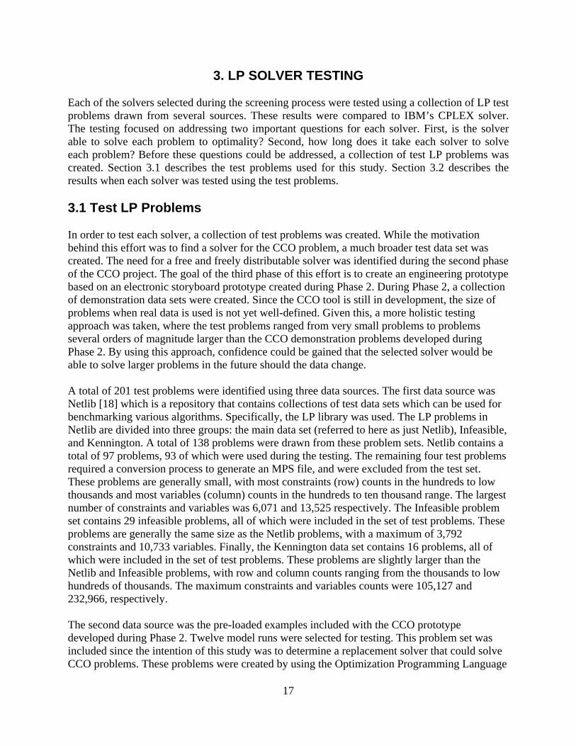
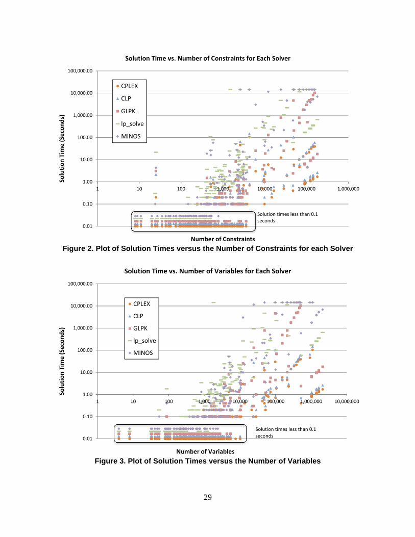
Times for Each Solver Finally, it is useful to look at the solution times for each problem based on the size of the problem. The three figures below show the solution times for each problem and solver by the number of constraints, variables, and non-zero elements in the problem. Given the range of problem sizes and solution times, all charts are presented using logarithmic scales for both axes. Additionally, since many problems had solution times that were rounded, and logarithmic charts cannot represent zeros, these problems are notionally represented by points within the boxes on each chart. For all points in the box, the size (x-axis value) is correct but the solution time (y-axis value) was zero. For lp_solve and MINOS, the problems that reached the maximum solution time of 14,400 seconds can be seen on each graph.
29
Figure 2. Plot of Solution Times versus the Number of Constraints for each Solver
Figure 3. Plot of Solution Times versus the Number of Variables
0.01
0.10
1.00
10.00
100.00
1,000.00
10,000.00
100,000.00
1 10 100 1,000 10,000 100,000 1,000,000
Solution Tim
e (Seconds)
Number of Constraints
Solution Time vs. Number of Constraints for Each Solver
Solution Time vs. Number of Variables for Each Solver
CPLEX
CLP
GLPK
lp_solve
MINOS
Solution times less than 0.1 seconds
30
Figure 4. Plot of Solution Times versus the Number of Non-zero Elements
Based on these results, it is clear that CLP performed the best in terms of its ability to accurately and efficiently solve problems. Both the Primal and Dual Simplex algorithms were able to solve all problems, and the geometric mean was only 1.6 times greater than the geometric mean for CPLEX. After CLP, the next best solver was GLPK. While the Dual Simplex algorithm failed to solve 9 problems within the allotted time, the Primal Simplex algorithm was able to solve all problems that could be read. The major drawback with GLPK was the solution time compared to CPLEX and CLP. The geometric mean for GLPK was 9.4 and 5.7 times greater than CPLEX and CLP, respectively. Despite this, GLPK appears to be a very capable solver which could be acceptable for use in applications where the increase in solve time is not a factor. The last two solvers, lp_solve and MINOS, had several drawbacks. First, both solvers encountered solve errors. In the case of lp_solve, only the Primal Simplex algorithm encountered these errors; the Dual Simplex algorithm was able to solve those problems. Second, both solvers were unable to solve all of the problems within the allotted time. Despite these errors, lp_solve and MINOS were still able to solve a large number of problems. These results suggest that more issues are likely to be encountered when using these solvers, especially when the problems being solved are difficult. 3.2.7 Results of “Hard” Problem Tests Based on the findings from the initial study, only CLP was tested using the “hard” problem set. The testing approach used for these problems was essentially the same as the initial test. Both the Primal and Dual Simplex algorithms were run for each problem and the best result was used. CLP’s default solver parameters were used and each problem was allowed eight hours to solve.
Solution Time vs. Number of Non‐zero Elements for Each Solver
CPLEX
CLP
GLPK
lp_solve
MINOS
Solution times less than 0.1 seconds
31
CPLEX was also used to solve the problems as a point of comparison. The “hard” data set contained 21 problems. Table 12 shows the solution times for each “hard” problem. Problem Rows Columns Best CLP Solution
Table 12. CLP and CPLEX Solution Times for “Hard” Problems. Italics indicate problems
that timed out. Bold indicates the fasted solver (CLP or CPLEX). CPLEX and CLP were able to solve 17 and 14 of the 21 “hard” problems, respectively. The CLP Dual Simplex algorithm timed out in seven cases and was stopped for numerical issues for one problem. The CLP Primal Simplex algorithm timed out for 10 problems. In all cases where CLP obtained an optimal answer, the relative error between the objective values for CLP and CPLEX was on the order of 1e-3 or less. If all 21 problems are considered, CLP and CLPEX required 217,475.5 seconds and 154,015.0 seconds to solve the problem set, respectively. CLP had a geometric mean of 1,004.2 seconds which was 2.5 times longer than the geometric mean of 402.2 seconds for CPLEX. If only the 14 problems solved by both solvers are considered, CLP and CLPEX required 15,875.5 seconds and 27,539.3 seconds, respectively, solving the problem set. In this case CLP was able to solve these problems faster than CPLEX, in terms of the total solution time. However, CLP had a geometric mean of 187.5 seconds, which was 1.74 times longer than the geometric mean of 112.6 seconds for CPLEX.
32
These results demonstrate some important points. First, since CPLEX was unable to solve 4 of these problems in 8 hours, it suggests that this test set contains problems that are sufficiently large to test the limits of both solvers. It also gives an indication of the size of the problems that can be handled by CLP. These results show that CLP can solve problems with about half a million constraints and just over 1 million variables. While CLP is generally slower, it was able to solve several of these problems in considerably less time than CPLEX. 3.2.8 Comments on LP Solver Testing Based on the results of the tests described above, CLP stood out as the open-source solver of choice. It demonstrated the ability to accurately solve problems in a short amount of time. It also demonstrated several other features which suggest it is a mature application. First, of all the solvers used in this study, it was the only one that was able to read all of the input files without any issues. Even CPLEX was unable to read five of the test problems initially and one of these read errors could not be corrected. CLP also had comparable performance to CPLEX, with respect to the time required to read each input file. CPLEX required 207.1 seconds to read 199 of the test problems (excludes FORPLAN.mps and OCS_MR_17.mps) and CLP required 209.2 seconds to read the same set of problems.
33
3. CONCLUSIONS The survey of open-source source LP solvers conducted for this study found that there are many options available when the use of commercial tools is not an option. Furthermore, testing demonstrated the capabilities of a subset of these solvers. While the primary goal of this study was to look at open-source solvers, it also demonstrates the value of using a commercial tool like CPLEX, as none of the open-source solvers were able to match its performance. However, this study also showed that capable open-source solvers are available when a tool like CPLEX is not an option. This study found that CLP was the best solver of those considered, in terms of capability and performance. GLPK is also a very capable solver, though it does not match the performance of CLP. lp_solve and MINOS had the slowest performance of the solvers considered and also encountered difficulties with a subset of the test problems. However, both of these tools are used in academia and can be purchased with commercial software, such as AMPL, and this study shows that they are able to handle many problems. Given this, all of the tools considered may work for problems of a certain size and difficulty. However, these results indicate that CLP is the tool of choice given the range of problems it can solve and the speed with which it can solve them.
34
35
4. REFERENCES
[1] International Business Machines Corporation, IBM ILOG CPLEX Optimization Studio v12.4, Armonk, 2011.
[2] J. Forrest and J. Hall, COIN-OR Linear Programming (CLP) v1.7.4, Computational Infrastructure for Operations Research (COIN-OR), 2008.
[3] J. Forrest and J. Hall, COIN-OR Linear Programming (CLP) v1.14.8, Computational Infrastructure for Operations Research (COIN-OR), 2012.
[4] A. Makhorin, GLPK (GNU Linear Programming Kit) v4.47.1, Moscow: Department for Applied Informatics, Moscow Aviation Institute, 2011.
[5] K. N. P. Eikland, lp_solve v5.5.2.0, 2010.
[6] MINOS v5.51, Palo Alto: Stanford Business Software Incorporated, 2002.
[7] R. Fourer, "Software Survey: Linear Programming," OR/MS Today, June 2011.
[8] "Wikipeida - Linear Programming," [Online]. Available: http://en.wikipedia.org/wiki/Linear_programming#Solvers_and_scripting_.28programming.29_languages. [Accessed 17 January 2013].
[9] "Solvers that Work with AMPL," [Online]. Available: http://www.ampl.com/solvers.html. [Accessed 17 January 2013].
[10] "GAMS Solver," [Online]. Available: http://www.gams.com/solvers/index.htm. [Accessed 17 January 2013].
[11] MINOS 5.5 Order Form (Government), Palo Alto: Stanford Business Software Incorporated.
[12] "AMPL," [Online]. Available: http://www.ampl.com/. [Accessed 19 April 2013].
[13] T. Magee, "Linear Programming: Alternatives to CPLEX," in 2006 RiverWare User Group Meeting, Boulder, 2006.
[14] B. Meindl and M. Templ, "Analysis of commercial and free open source solvers for linear optimization problems," Essnet Project on Common Tools and Harmonized Methodologies for SDC in the ESS, 2012.
[15] H. Mittelmann, "Benchmark for Optimization Software," [Online]. Available: http://plato.asu.edu/bench.html. [Accessed 17 January 2013].
[16] "COIN-OR," [Online]. Available: http://www.coin-or.org/index.html. [Accessed 17 January 2013].
[17] "CLP FAQ," [Online]. Available: https://projects.coin-or.org/Clp/wiki/FAQ. [Accessed 17 January 2013].
[18] J. Dongarra and E. Grosse, "Netlib," [Online]. Available: http://www.netlib.org/. [Accessed 17 January 2013].
36
37
APPENDIX A: LP TOOL SCREENING This appendix lists all of the tools that were considered during the initial LP software survey. For each tool, a decision was made to include or reject it from the second round of screening. For those tools that were rejected, the reason is provided in each of the tables below. Comments are also provided for tools that were identified as candidate tools. Not all of the tools that were accepted were LP solvers. Open-source tools such as modeling environments or integer program solvers were accepted in the initial round of screening. They were not considered as part of this study since they address a different need; however they are highlighted here since they are open-source tools that may be useful in another application. Table 13 lists the tools described in the INFORMS survey [7].
Product Candidate Tool
Reason Rejected Comments
AIMMS N $8,500 per license AMPL N $4,000 per license, only provides
modeling environment
CBC Y IP solver that uses CLP (a LP solver) while not useful for this application this tool might be of general interest.
CLP Y LP Solver CoinMP Open-Source Solver
Y Not an LP solver but potentially useful as a modeling environment
Coopr Y Not an LP solver but potentially useful as a modeling environment
C-WHIZ N $2,500 per license DATAFORM N $2,500 per license; Data
management tool (not relevant)
FICO Xpress Optimization Suite
N Commercial software
Frontier Analyst 4
N 4,000GBP per license
GAMS N $3,200 per license GENO N Not free; Genetic algorithm GIPALS - Linear Programming Environment
N $150-300; Immature
Gipals32 - Linear
N $150-300; Immature
38
Programming Library GLPK (GNU Linear Programming Kit)
Y LP Solver
Gurobi Optimizer 4.5
N Not free
IBM ILOG CPLEX Optimization Studio
N Not free
KNITRO N Not free LINDO API N Not free LINGO N Not free LOQO N Not free Mathematical Modeling System
N Not free
Microsoft Solver Foundation
Y Not an LP solver but potentially useful as a modeling environment
MOSEK N Not free MPL Modeling System
N Not free
OML (Optimization and Modeling Library)
N Not free
OMP Plus N Not free OptiMax Component Library
N Not free
OptimJ Y Not an LP solver but potentially useful as a modeling environment
Oracle Crystal Ball Suite
N Not free; Monte Carlo algorithm
PICO N Questionable reliability Premium Solver Platform
N Excel Solver
Premium Solver Pro
N Excel Solver
QMS N Not free
39
Risk Solver Platform
N Excel Solver
SAS N Not free SCIP N Not free for non-academic uses Solver SDK Platform
N Not free
Solver SDK Pro N Not free SoPlex N Not free for non-academic uses SOPT (Smart Optimizer) 4.2
N Not free
Vanguard Global Optimizer
N Not free
What'sBest! N Not free XA N Not free YALMIP N MATLAB add-in
Table 13. First Round Screening Results for Tools Listed in INFORMS LP Software
Survey [7] Table 14 lists the proprietary tools listed on the Wikipedia page for Linear Programming [8]. Proprietary tools were considered during the survey because some tools offer government pricing and flexible licensing which may still meet the criteria. This source was used only to identify candidate tools. All screening decisions were based on information gathered by reviewing the official documentation for each tool. Product Candidate
Tool Reason Rejected Comments
APMonitor N Not relevant AIMMS N $8,500 per license AMPL N $4,000 per license, only provides
modeling environment
Analytica N Not free BUGSENG Polyhedra Library
Y LP Solver
CPLEX N Not free EXCEL Solver Function
N Excel tool
FinMath N Not free FortMP N Not free GAMS N Not free GIPALS N Not free Gurobi N Not free
40
IMSL Numerical Libraries
N Not free
Lingo N Not free LPL N Information on tool could not be
found
LiPS (freeware)
Y LP Solver
MATLAB N Not free Mathematica N Not free MOPS N Information on tool could not be
found
MOSEK N Not free NAG Numerical Library
N Not free
NMath Stats N Not free
OptimJ Y Not an LP solver but potentially useful as a modeling environment
SAS/OR N Not free SCIP N Not free for non-academic use Microsoft Solver Foundation
Y Not an LP solver but potentially useful as a modeling environment
SoPlex N Not free SuanShu N Not free TOMLAB N MATLAB add-in VisSim N Not relevant Xpress N Not free
Table 14. First Round Screening Results of Propriety LP Tool from Wikipedia [8] Table 15 lists the non-proprietary tools listed on the Wikipedia page on Linear Programming [8]. This source was used only to identify candidate tools. All screening decisions were based on information gathered by reviewing the official documentation for each tool. Product Candidate
Tool Reason Rejected Comments
lp_solve Y LP Solver
Cassowary constraint solver
N Immature
41
CVXOPT Y Quadratic program solver
glpk Y LP solver PPL Y LP solver and quadratic
program solver Qoca N Immature CBC Y IP solver that uses CLP
(a LP solver) while not useful for this application this tool might be of general interest.
CLP Y LP Solver R-Project N Not relevant CVX N MATLAB add-in CVXMOD N Immature SDPT3 N MATLAB add-in SeDuMi N MATLAB add-in OpenOpt Y Not an LP solver but
potentially useful as a modeling environment
pulp-or N Not an LP solver but potentially useful as a modeling environment
Pyomo (Coopr)
N Not an LP solver but potentially useful as a modeling environment
JOptimizer Y LP solver
Table 15. First Round Screening Results of Non-propriety LP Tool from Wikipedia [8] Table 16 lists additional tools that were discovered by looking at a variety other linear programming websites [9] , [10]. Product Candidate Tool Reason Rejected Comments BARON N Only available with
commercial software
BDMLP N Only available with commercial software
LOGMIP N Immature OSL N Discontinued IBM product MOP N Information on tool could not
be found
LSGRG2 N Information on tool could not
42
be found BPMPD N Immature MINTO Y IP solver that uses CLP or
CPLEX (LP solvers) while not useful for this application this tool might be of general interest.
OOQP Y Quadratic program solver PCx Y LP solver QPOPT Y Quadratic program solver QSOPT Y LP solver CMPL Y Not an LP solver but
potentially useful as a modeling environment
MINOS Y LP solver GMPL Y Not an LP solver but
potentially useful as a modeling environment
LSSOL Y Quadratic program solver
Table 16. First Round Screening Results from a General Survey of LP Websites
43
APPENDIX B: OPEN-SOURCE LP MODELING ENVIRONMENTS In addition to surveying open-source LP solvers, a parallel study was conducted to look for open-source modeling environments. As mentioned in Section 2.1, it is difficult to create problem statements using a solver’s API. Modeling environments allow problems to be written in a concise and easy to read manner. Modeling environments also offer the added benefits that they can connect to several solvers and are extensions to standard programming languages. This provides the flexibility to switch solvers while maintaining a single implementation of the model. It also means that all the features of programming languages, such as database connections, can be used when creating models. While details of this study are outside the scope of this report, Table 17 lists the top open-source modeling environments that were identified during that study. Note that Microsoft Solver Foundation was included on this list even though it is not an open-source product. Since many organizations have Microsoft Development licenses, this tool may still be a good option that is considerably less expensive than a modeling environment like AMPL [12].
Environment Language API Command Line Interface
Supported Solvers
CMPL C++ N Y CPLEX, CLP, GLPK, Gurobi, SCIP
Coopr Python Y Y CPLEX, CLP, GLPK, Gurobi, AMPL Solver Library
OptimJ Java Y N CPLEX, lp_solve, GLPK, Gurobi, Mosek
PuLP Python Y N CPLEX, CLP, GLPK, Gurobi
Microsoft Solver Foundation
.NET Y N CPLEX, CLP, FICO, Gurobi, LINDO, lp_solve, Mosek, Ziena, Frontline
FLOPC++ C++ Y N CPLEX, CLP, Dylp, GLPK, OSL, SOPLEX, VOL, XPRESS-MP
Table 17. List of Top Open-Source LP Modeling Environments. Solvers studied in this
model are highlighted in bold. Other open-source solvers are italicized.
For the purposes of this study, the most important information can be found in the last column. Observe that all of these tools support some combination of CLP, GLPK, and lp_solve. The fact that the top modeling environments have chosen to support these solvers suggests that these solvers are used by a sufficiently large community and that they are reasonably well developed. The solvers shown in italics are other open-source solvers (not CLP, GLPK, or lp_solve). Observe that outside of CLP, GLPK and lp_solve, no other open source solver is supported by more than one modeling environment. This suggests that no other open-source solvers have the same level of acceptance with the modeling environment community.
44
45
APPENDIC C: LIST OF TEST PROBLEMS Table 18 lists all of the test problems, as well as their size, the problem set they belong to, and the published optimal objective value if known. All problems were minimization problems. All problems except for the Small and Large CCO problems were in the MPS format. The CCO problems were created in the Free MPS format. After CPLEX, CLP, and GLPK were tested, MPS versions of these files were created and used to test lp_solve and MINOS.
CCO_MR_31_CLP.mps 1,608 2,954 28,621 Small CCO N/A
CCO_MR_35_CLP.mps 1,695 3,244 29,256 Small CCO N/A
CCO_MR_33_CLP.mps 1,701 3,279 29,275 Small CCO N/A
CCO_MR_36_CLP.mps 1,715 3,272 29,312 Small CCO N/A
CCO_MR_37_CLP.mps 1,715 3,272 29,312 Small CCO N/A
CCO_MR_32_CLP.mps 2,272 4,226 52,435 Small CCO N/A
CCO_MR_14_CLP.mps 2,449 4,629 53,254 Small CCO N/A
CCO_MR_15_CLP.mps 2,483 4,886 53,625 Small CCO N/A
CCO_MR_17_CLP.mps 2,606 5,258 54,181 Small CCO N/A
CCO_MR_13_CLP.mps 2,674 4,824 70,563 Small CCO N/A
CCO_MR_27_CLP.mps 2,674 4,824 70,563 Small CCO N/A
CCO_MR_28_CLP.mps 2,889 5,414 71,599 Small CCO N/A
CCO_MR_31.mps 47,522 517,971 833,978 Large CCO N/A
CCO_MR_33.mps 90,290 1,031,187 1,465,994 Large CCO N/A
CCO_MR_35.mps 90,290 1,031,187 1,465,994 Large CCO N/A
CCO_MR_36.mps 90,290 1,031,187 1,465,994 Large CCO N/A
CCO_MR_37.mps 90,290 1,031,187 1,465,994 Large CCO N/A
CCO_MR_14.mps 123,123 1,406,164 2,187,003 Large CCO N/A
CCO_MR_15.mps 123,123 1,406,164 2,238,843 Large CCO N/A
CCO_MR_32.mps 123,123 1,406,164 2,187,003 Large CCO N/A
CCO_MR_13.mps 143,643 1,640,524 2,570,403 Large CCO N/A
CCO_MR_27.mps 143,643 1,640,524 2,570,403 Large CCO N/A
CCO_MR_28.mps 143,643 1,640,524 2,570,403 Large CCO N/A
50
CCO_MR_17.mps 181,443 2,106,004 3,048,843 Large CCO N/A
Table 18. Listing of Test LP Problems
51
APPENDIX D: TEST PROBLEM READ ERRORS Before algorithm testing was started, a set of tests were conducted to ensure that each problem could be read by every solver. While the MPS format is the standard text input format for LP solvers, there are some variations within this format. For example, comments and blank lines within an MPS file cause issues with some solvers. Since the intention was to create a common set of test problems, every effort was made to correct read errors provided that it did not change the problem (i.e. while removing comments would be acceptable, changing data would not). With the exception of MINOS, all solvers provided an import feature that allowed the model to be read without being solved. CPLEX CPLEX encountered an error while reading the following problems: DFL001.mps, SIERRA.mps, GFRD-PNC.mps, FORPLAN.mps, and BLEND.mps. With the exception of FORPLAN.mps, all of these read errors were corrected by having lp_solve import these models then create a new copy of the model through an export. The cause of the read error for FORPLAN.mps could not be determined and this model was not solved by CPLEX. CLP CLP did not encounter any read errors. GLPK GLPK encountered read errors on the following problems during the import tests: GREENBEA.mps, PANG.mps, DFL001.mps, SIERRA.mps, GFRD-PNC.mps, FORPLAN.mps, and BLEND.mps. With the exception of PANG.mps and FORPLAN.mps, all of these errors were corrected by using lp_solve to import then export a new MPS file. The cause of the read errors for PANG.mps and FORPLAN.mps could not be determined, however, GLPK was able to read and solve these problems during the algorithms testing. During the algorithms testing, GLPK was unable to read any of the five Rail problems, despite the fact that they could be read during the import tests. The cause of this read error is unknown. lp_solve lp_solve encountered read errors while attempting to read all of the CCO problems in the Free MPS format, despite the fact that lp_solve can accept this format. This error was corrected by using the import feature for CLP to import these files as Free MPS problems and export them as MPS problems. MINOS Unlike the other solvers, MINOS does not offer an import feature. Therefore the read capability of MINOS was tested with the algorithm testing. Since MINOS was not tested using the “hard”
52
problems, only the 180 “easy” problems were read. Since MINOS only accepts MPS files, it was known in advance that the CCO problems in the Free MPS format could not be solved. However, MINOS was able to read the CCO problems after they were converted to the MPS format and read all other “easy” problems with no issues.
53
APPENDIX E: COMPARISON OF CLP 1.7.4 AND 1.14 The purpose of this appendix is to describe the results of a test to compare CLP version 1.7.4 to CLP version 1.14 [2], [3]. CLP 1.7.4 was used during the original LP solver testing, since it was the last version for which the COIN-OR Binaries project offered a compiled 64-bit Windows application. Since this version of CLP was several years old, there was a desire to use a more current version. The most current version of CLP is 1.15; however CLP version 1.14 was selected for this comparison. At the time that this test was started, CLP version 1.15 was only a few days old. Given this, the decision was made to use the previous release. The approach used for this test was to rerun the “easy” and “hard” test problems for the Primal and Dual Simplex algorithms using the new version of CLP and compare the results to the previous version of CLP. The primary concerns of this test were to ensure that the new version of the algorithm reached the correct optimal value for each problem and that the solution times were about the same. As in the original LP solver tests, all timing results were rounded to the nearest tenth prior to performing any calculations, unless otherwise stated. Geometric means are reported using the lowest level of precision possible since zeros cannot be included in the calculation: three digits when comparing CLP results and two digits when comparing CPLEX results. Based on the results of this test both versions of the solver were determined to be comparable in their overall performance. The new version of CLP was slower than the original version of CLP that was tested. However, there have been many updates and bug fixes since CLP 1.7.4, and the new version of CLP was able to solve some problems that could not be solved by CLP and CPLEX during the original testing. Given these results, it was determined that CLP 1.14 can be used in place of CLP 1.7. Results for “Easy” Test Problems This section describes the comparison of the results for the “easy” test problems. The results were considered in three different ways. The first two comparisons are between the primal and dual results for CLP 1.14 to the respective results for CLP 1.7. The third comparison is between the best results between the both algorithms for both versions of CLP. This last comparison is the same approach that was used in the original testing. The original testing did not compare primal results to primal results, and dual results to dual results, however this is done here since the intention of this test is to ensure that both the Primal and Dual Simplex algorithms perform the same or better. The first test was to compare the Dual Simplex algorithm results for both versions of CLP. The new version of CLP was able to solve all 180 problems, just as CLP 1.7.4 was. Initially, CPLEX2.mps was incorrectly identified as feasible. However, once the tolerance settings were adjusted, CLP version 1.14 identified it as infeasible. This was interesting because, in the original test, CLP 1.7.4 correctly solved this problem using the Dual Simplex algorithm but required tolerance setting adjustment to solve it correctly, using the Primal Simplex algorithm. For the new version of CLP, the Primal Simplex algorithm was able to solve this problem correctly, but the Dual Simplex algorithm required adjustments to the tolerances settings. As
54
with the original test, this was not treated as an error with the solver since the issue was correctable and appears to be specific to this problem. The new version of CLP correctly identified all of the infeasible problems. For all but 2 of the 151 problems with feasible solutions, the optimal objective values were the same. The remaining two problem’s objective values were essentially the same with relative errors on the order of 1e-8 or less. These results show that the Dual Simplex algorithm in both versions of CLP produces the same results. The new version of CLP generally takes longer to solve the “easy” problems using the Dual Simplex algorithm. Table 19 gives the total time to solve the each of the “easy” problem sets using the Dual Simplex algorithm in CLP 1.7.4 and CLP 1.14. While the total solution time is shorter using the new version of CLP, the geometric mean (using the three-digit timing precision) shows a 31.7% increase in the solution times using CLP 1.14. In terms of the total solution time, there were substantial increases for the Infeasible, Plato – PDS, and Large CCO problems sets. Essentially all of the increase in the Large CCO problem set solution time can be attributed to an increase in the pre-solve time. The exact cause of this is unknown. It is also worth noticing that the total solution time for the Small CCO problem decreased slightly. Since the intention is to construct the CCO problem without the unnecessary constraints in the Large CCO problems, there should be minimal increases in the solution time of the CCO problem due to the pre-solver.
Problem Set Sum of CLP 1.7.4 Solve Times (Seconds)
Sum of CLP 1.14 Solve Times (Seconds)
Infeasible 3.9 18.3 Kennington 17.0 20.0 NetLib 31.9 28.6 Plato - FOME 182.7 179.5 Plato - PDS 224.5 455.2 Plato - Rail 4,821.8 4,171.0 Large CCO 19.0 378.0 Small CCO 0.1 0.0 Grand Total 5,300.9 5,250.6
Table 19. Comparison of Total Solution Times (Seconds) for Each “Easy” Problem Set
Using the Dual Simplex Algorithms for CLP 1.7.4 and CLP 1.14 The second test was to compare the Primal Simplex algorithm results for both versions of CLP. The new version of CLP was able to solve all 180 problems. This is an improvement over the Primal Simplex algorithm for CLP 1.7.4, which was unable to solve OCS_MR_17.mps and initially identified CPLEX2.mps as feasible. Again, this was interesting because, in the original test, CLP 1.7.4 correctly solved this problem using the Dual Simplex algorithm but required tolerance setting adjustment to solve it correctly using the Primal Simplex algorithm. For the new version of CLP, the Primal Simplex algorithm was able to solve this problem correctly but the Dual Simplex algorithm required adjustments to the tolerances settings. The new version of
55
CLP correctly identified all of the infeasible problems. For all but 4 of the 151 problems with feasible solutions, the optimal objective values were the same. The remaining four problem’s objective values were essentially the same, with relative errors on the order of 1e-8 or less. These results show that the Primal Simplex algorithm was able to match all of the results for the problems solved during the initial test and solve one problem that could not solved by CLP 1.7. CLP 1.14 appears to solve the “easy” problems slightly faster using the Primal Simplex algorithm than CLP 1.7. Table 20 gives the total time to solve the each of the “easy” problem sets using the Primal Simplex algorithm in CLP 1.7.4 and CLP 1.14. Using the three-digit timing precision, the total solution time is about 47.1% shorter using the new version of CLP. The geometric mean is about 2.8% shorter using the new version of CLP. In terms of the total solution time, all of the problem sets, except for Large CCO, were solved quicker using CLP 1.14. As with the Dual Simplex algorithm for CLP 1.14, the increase in the total solution time for the Large CCO problems can be attributed to an increase in the pre-solve time. It is also worth noticing that the total solution time for the Small CCO problem decreased slightly. Since the intention is to construct the CCO problem without the unnecessary constraints in the Large CCO problems, there should be minimal increases in the solution time of the CCO problem due to the pre-solver.
Problem Set
Sum of CLP 1.7.4 Solve Times (Seconds)
Sum of CLP 1.14 Solve Times (Seconds)
Infeasible 8.1 4.5 Kennington 108.2 56.6 NetLib 61.6 41.1 Plato - FOME 522.4 368.5 Plato - PDS 7,351.6 3,400.8 Plato - Rail 212.9 132.7 Large CCO 16.7 377.8 Small CCO 1.0 0.0 Grand Total 8,282.5 4,382.0
Table 20. Comparison of Total Solution Times (Seconds) for Each “Easy” Problem Set
Using the Primal Simplex Algorithms for CLP 1.7.4 and CLP 1.14 For the final test, the results from the Primal and Dual Simplex algorithms were combined to determine the best possible solution times for each problem. These results were compared for both versions of CLP. This is the same approach that was used during the original tests. For this test only the solution times were compared since it was previously established that both algorithms were able to accurately solve all of the “easy” test problems. Table 21 shows the total solution times for CPLEX, CLP 1.7.4 and CLP 1.14, for each problem set. The total solution time for CLP 1.14 was about 20 minutes, compared to 11.5 minutes for CLP 1.7.4, and 7 minutes for CPLEX. Using two digits of timing precision, the geometric mean of solution times using
56
CLP 1.14 was 2.07 times greater than CPLEX and 1.41 times greater than CLP 1.7. Observe that CLP 1.14 was able to solve the Plato – Rail problem set faster than CPLEX or CLP 1.7.4, but otherwise matched the solution times of CLP 1.7.4 or did worse. CLP 1.14 also includes a new feature which attempts to select the best algorithm (between the primal and dual) automatically for the user. A side test was conducted to test this feature. When the “easy” test problems were run with this feature turned on, CLP 1.14 was able to solve all of the problems in about 20 minutes. This matches the total solution time that was required when the best results from the primal and dual were combined. This simple test suggests that this feature does a good job of selecting the fastest algorithm.
Table 21. Comparison of Total Solution Times (Seconds) for Each “Easy” Problem Set
Using CPLEX, CLP 1.7.4, and CLP 1.14 Results for “Hard” Test Problems CLP 1.14 was also tested using the “hard” test problems. The testing approach used for these problems was the same as the approached used for the “easy” test problems. First, the dual results for both versions of CLP were compared, and then the primal results for both versions of CLKP were compared. Finally, the primal and dual results were combined and best results from each algorithm were compared. The Dual Simplex algorithm in CLP 1.14 was used to solve the 21 “hard” test problems. Using this algorithm, 13 of the problems could be solved within the allotted time. Seven problems timed out and one problem was stopped for numerical reasons. This exactly matches the results from the original test using CLP 1.7. For those problems that could be solved, the total solution time increased from 4.7 hours to 5.6 hours, and the geometric mean (using the three-digit timing precision) increased by 20%.
57
The Primal Simplex algorithm in CLP 1.14 was able to solve 13 of the problems. This is an improvement over the Primal Simplex algorithm in CLP 1.7.4, which was only able to solve 11 of the problems. For CLP 1.7.4, the ten problems that failed to solve all reached the maximum time limit. CLP 1.14 was able to solve two of these problems and timed out on the same remaining eight problems. Interestingly, one of the two problems that CLP 1.14 was able to solve, cont11_I.mps, was identified as infeasible and solved in 311 seconds. Neither, CLP 1.7.4 or CPLEX was able to solve this problem within the 8 hour time limit. If the eight problems that could not be solved are ignored, the total solution times for CLP 1.14 and CLP 1.7.4 are 7.3 hours and 19.9 hours, respectively. In this case the geometric mean of solution times for CLP 1.14 is 58% shorter than CLP 1.7. If only the 11 problems that both solvers could solve are considered, the total solution times for CLP 1.14 and CLP 1.7.4 are 6.4 hours and 3.9 hours, respectively. Despite the fact that CLP 1.14 takes longer to solve, in terms of the total solution time, its geometric mean is actually 33% shorter then CLP 1.7. For the final test, the results from the Primal and Dual Simplex algorithms were combined to determine the best possible solution times for each problem. These results were compared for both versions of CLP. This is the same approach that was used during the original tests. Table 22 summarizes the results for CPLEX, CLP 1.7.4 and CLP 1.14. All geometric means were computed using two digits of timing precision. Since each of these solvers was able to solve a different set of problems, the results are presented in three different ways. First, the results for all 21 “hard” test problems are shown, then the results for the 18 problems that could be solved by at least one of the solvers are shown, and finally the results for the 14 problems that could be solved by at least one of the solvers are shown. Observe that, in terms of the geometric mean, CLPEX is always the fastest solver. For the first two groups of statistics, CLP1.14 is faster than CLP 1.7. When only the 14 problems that could be solved by all solvers are considered, the geometric mean for CLP 1.14 is about 7% larger than CLP 1.7’s geometric mean. Summary of Changes since CLP 1.7.4 In addition to testing the algorithms, a review of the subversion commit messages since the CLP version 1.7.4 was accomplished to get a sense of the types of modifications that have been made. A complete listing of the revisions to the CLP source code is available at: https://projects.coin-or.org/Clp/log/. The commit revisions of interest range from 1195 to 1889. The first change to CLP version 1.7.4 occurred on April 16, 2008. Change 1889 occurred on November 21, 2012. Based on the commit messages, it appears that a variety of changes have been made. There have been updates to correct memory leaks, fix mistakes with the algorithms, and improve the performance of the algorithms. Based on the commit messages, most of these changes appear to be fixes to minor bugs. However, there were two commit messages that are worth pointing out. The message for revision 1498 stated: “fix serious - if rare - bug which says optimal when not”. Since the optimal objective values were reached for the entire test problem set during the original testing, it does not appear that CLP 1.7.4 encountered this bug. The message for revision 1575 stated: “Added OSI into externals”. This is important because the COIN-OR Open Solver Interface (OSI) was not available until this point in time. Without this, an interface tool such as FLOPC++ cannot be used to directly interface with CLP (using these tools to write an MPS input file for CLP is still an option).
58
CPLEX CLP 1.7.4 CLP 1.14 All 21 "Hard" Problems Total Time (Hours) 42.8 60.4 51.8 Geometric Mean 402.1 1,004.4 846.3 Ratio to CPLEX 2.50 2.10 CLP 1.14 Ratio to CLP 1.7 0.84 18 Problems Solved by One Solver Total Time (Hours) 18.8 36.4 27.8 Geometric Mean 197.3 574.1 470.1 Ratio to CPLEX 2.91 2.38 CLP 1.14 Ratio to CLP 1.7 0.82 14 Problems Solved by All Solvers Total Time (Hours) 7.6 4.4 3.7 Geometric Mean 112.5 187.6 200.5 Ratio to CPLEX 1.67 1.78 CLP 1.14 Ratio to CLP 1.7 1.07
Table 22. Various Statistics Comparing CPLEX, CLP 1.7.4, and CLP 1.14 for the “Hard”
Test Problems Conclusion Based on this analysis, it was determined that CLP 1.14 is suitable for use in place of CLP 1.7. The testing shows that both the Primal and Dual Simplex algorithms are able to achieve the correct optimal objective values. The results do indicate that, in some cases, using CLP 1.14 instead of CLP 1.7.4 increases the solution time by 30-40%. However, the new version of CLP was able to solve three problems that CLP 1.7.4 could not solve and one problem that CPLEX could not solve. Additionally, the commit messages indicate that many bugs have been fixed since the release of CLP 1.7. Despite the fact that CLP 1.14 generally requires more time to solve the test problems, the solution time for the Small CCO problems did not increase. Furthermore, CLP 1.14 is still a very efficient solver when compared to CPLEX, requiring about 2.1 times as long to solve the “easy” test problems, compared to 1.6 times as long for CLP 1.7. Given that CLP 1.14 was able to solve more of the test problems, and that many bugs have been corrected since CLP 1.7.4 was released, the improvements in capability offset this increase in processing time.