Page 1
Comparison of various fluid-structure interaction methods for
deformable bodies.
R. van Loon1∗ , P.D. Anderson2, F.N. van de Vosse3, S.J. Sherwin1
1 Department of Aeronautics, Imperial College London,
South Kensington Campus, SW7 2AZ, London, UK
2 Department of Mechanical Engineering, Eindhoven University of Technology,
P.O. Box 513, 5600 MB, Eindhoven, The Netherlands
3 Department of Biomedical Engineering, Eindhoven University of Technology,
P.O. Box 513, 5600 MB, Eindhoven, The Netherlands
∗E-mail: [email protected] Tel: +44 (0)20 75945129
1 Abstract
A perspective is given on fictitious domain methods for deformable bodies that exert large motions
induced by unsteady flow. In these methods an Eulerian and Lagrangian formulation are employed
for the fluid and solid, respectively, and both bodies are coupled using a Lagrange multiplier. This
multiplier allows the solid not to be an integral part of the fluid mesh, that therefore requires
no updating. Three variations of the fictitious domain method that have been published before,
are compared to an ALE method in two numerical experiments and in conclusion the advantages,
disadvantages and differences for the different approaches are regarded.
Keywords: fluid-structure interaction; FSI; fictitious domains; ALE; deformable solids; Lagrange
multipliers
2 Introduction
In a finite element, finite difference or finite volume setting, the fluid domain is generally described
in an Eulerian frame of reference obtaining solutions in grid/mesh points that are fixed in space.
1
Page 2
Although this approach works well for a geometrically fixed fluid domain, difficulties arise when
the fluid domain changes shape or when moving interfaces are present inside the domain. Typical
examples are flow through flexible tubes, swimming fish, moving cilia, a functioning heart valve
or a flapping flag. Different techniques have been proposed and investigated for handling moving
interfaces and in particular the interfaces of an elastic solid structure embedded in a fluid.
One of the most well-known methods used to capture the interaction between structure and
fluid is the Arbitrary Lagrangian Eulerian method (ALE). An Arbitrary Lagrangian Eulerian
method allows arbitrary motion of grid/mesh points with respect to their frame of reference by
taking the convection of these points into account as described in Hirt et al. (1974), Donea et al.
(1982), Hughes et al. (1981) and many works thereafter. In the case of an FSI problem, the
fluid points at the fluid-solid interface are moved in a Lagrangian way. Since the method is easy
to implement, has low computational cost and is accurate, it is recommendable to use whenever
possible. However, for large translations and rotations of the solid or inhomogeneous movements of
the grid/mesh points fluid elements tend to become ill-shaped, which reflects on the accuracy of the
solution. Remeshing, in which the whole domain or part of the domain is spatially rediscretised,
is then a common strategy. The process of mesh generation multiple times during a computation
can, however, be a very troublesome and time consuming task. Furthermore, the transfer of
solutions from the degenerated mesh to the new mesh may introduce artificial diffusion, causing
loss of accuracy.
Opposed to the ALE technique where the fluid-solid interface is accurately captured other
types of methods do not require any changes of the fluid mesh/grid. A widely used non-boundary-
fitting method for FSI applications is the immersed boundary method , which was proposed by
Peskin (1972, 2002). The first models consider a finite difference grid for the fluid domain with an
immersed set of non-conforming boundary points, that are mutually interconnected by an elastic
law. This solid boundary interacts with the fluid by means of local body forces applied to the
fluid at the position of the points. This body force imposes the kinematic constraint that the
velocity in each of these solid point is coupled to the (interpolated) fluid velocity at that point.
The introduction of these body forces has become the basic idea behind several non-boundary-
fitting FSI methods. Throughout the years, the Immersed Boundary Method has been successfully
applied in many application fields (Peskin and McQueen, 1989; Dillon and Fauci, 2000a; Zhu and
Peskin, 2002; Gilmanov and Sotiropoulos, 2005).
Another method closely related to the the immersed boundary method, is the so-called ficti-
2
Page 3
tious domain method (Glowinski et al., 1997). Unlike the immersed boundary method that was
developed within a finite difference framework, the fictitious domain method evolved from the field
of finite elements. Coupling is established by constraining fluid and rigid body at the interface
using a (distributed) Lagrange multiplier and extending this constraint to the inner body. In the
strong form the fictitious domain method is not different from the immersed boundary method
method, only by applying the multipliers (which represent the body forces) in the weak form the
forces are imposed in a distributed manner using an integral formulation.
Based on the fictitious domain idea Baaijens (2001) proposed a fluid-solid interaction version
suitable for slender bodies. In this work a fluid and solid mesh are generated independently from
each other and both domains are coupled by means of a Lagrange multiplier along the boundary of
the solid. The solid is described in a Lagrangian way, deforming under the acting fluid forces, while
the Eulerian fluid mesh does not require updating. This method has been successfully applied in
flexible heart valve simulations (De Hart et al., 2000, 2003).
A disadvantage of Baaijens’ technique is that it is only applicable to slender bodies. Several
extended versions have since been proposed where non-slender elastic solid bodies are coupled
across the whole body instead of a boundary, which broadens the application field. The Extended
Immersed Boundary Method (Wang and Liu, 2004) and the Immersed Finite Element Method
(Zhang et al., 2004) describe the solid using the finite element method while the fluid is formulated
using a finite difference or finite element method, respectively. The coupling is performed using
the discrete dirac delta functions that find their origin in the meshless reproducing kernel particle
method (RKPM). Examples include the dropping of rigid or deformable particles in a three-
dimensional channel. Yu (2005) set out his version of the fictitious domain method for non-
slender deformable bodies. Analysis of this approach was performed by two numerical examples:
the motion of a slender solid slab in a pulsatile flow (like the one in Baaijens (2001)) and the
self-sustained flapping of a slender solid in a constant flow (like in Zhu and Peskin (2002)).
The non-boundary-fitting methods have a reduced accuracy for the solution near the fluid-
solid interface due to interpolation and in the ALE methods the fluid elements tend to get ill-
shaped requiring difficult and expensive meshing. Therefore, another variation on the distributed
Lagrange multiplier principle was proposed by Van Loon et al. (2004). A combination of the two
might lessen their disadvantages without losing too much of the benefits. The approach consisted
of the fictitious domain method similar to that of Baaijens, but extended with an ALE step and a
local adaptive meshing algorithm for the fluid mesh (Van Loon et al., 2006). Due to the use of the
3
Page 4
Lagrange multiplier the meshes did not have to be conforming at the solid-fluid interface, which
allowed the meshing algorithm to be simple and very local. To show the improved accuracy, shear
stresses along both sides of the solid were computed.
The aim of this work is to provide a comparison between different FSI methods that can be
used for slender deformable bodies in a fluid. Comparing existing methods that have been pre-
sented in different works is always a tedious matter due to variations in discretisations, geometry,
polynomial order or boundary conditions used in the different publications that might influence
the comparison. We made an effort to restrain these parameters for a more specific focus on the
FSI itself. The chosen approaches all fall within the finite element type of methods and each
approach with its advantages and disadvantages will be highlighted. The more conventional ALE
method and three variations of the fictitious domain methods will be considered in two numerical
experiments. The fictitious domain methods are the ones earlier proposed by Baaijens (2001), Yu
(2005) and Van Loon et al. (2006). This way we hope to provide more insight in the strengths
and, possibly more important, the weaknesses of the various methods.
3 Methods
3.1 Governing Equations
First the governing equations for a fluid-structure interaction problem in the strong form are
considered. The momentum balances that hold in fluid domain Ωf and solid domain Ωs are
presented and, additionally, incompressibility of both media is enforced by a continuity constraint
for the fluid and an volumetric constraint for the solid. The superscripts ’s’ and ’f ’ are used in
this work to indicate if a quantity belongs to the solid or to the fluid, respectively.
Fluid:
ρf ∂uf
∂t+ ρfuf · ∇uf = ∇ · σf + ρff f , in Ωf (1)
∇ · uf = 0, in Ωf (2)
σf = 2ηD − pfI in Ωf (3)
4
Page 5
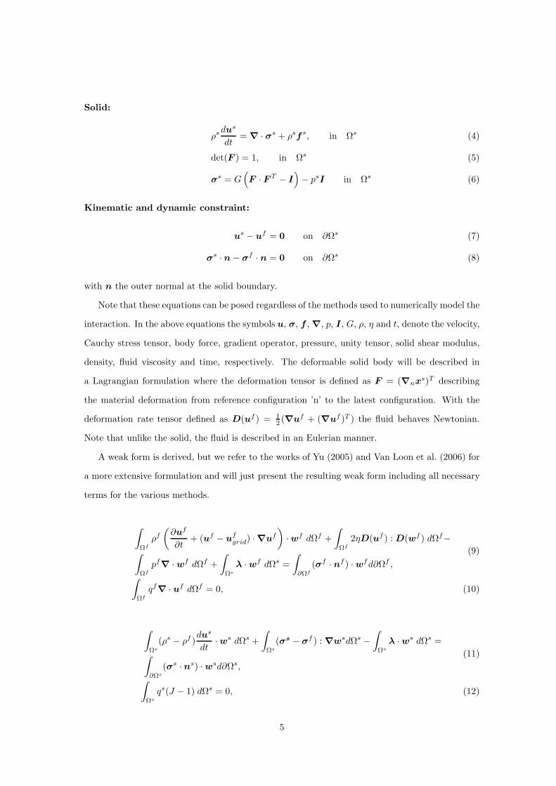
Solid:
ρs dus
dt= ∇ · σs + ρsf
s, in Ωs (4)
det(F ) = 1, in Ωs (5)
σs = G(
F · F T − I)
− psI in Ωs (6)
Kinematic and dynamic constraint:
us − uf = 0 on ∂Ωs (7)
σs · n − σf · n = 0 on ∂Ωs (8)
with n the outer normal at the solid boundary.
Note that these equations can be posed regardless of the methods used to numerically model the
interaction. In the above equations the symbols u, σ, f , ∇, p, I, G, ρ, η and t, denote the velocity,
Cauchy stress tensor, body force, gradient operator, pressure, unity tensor, solid shear modulus,
density, fluid viscosity and time, respectively. The deformable solid body will be described in
a Lagrangian formulation where the deformation tensor is defined as F = (∇nxs)T describing
the material deformation from reference configuration ’n’ to the latest configuration. With the
deformation rate tensor defined as D(uf ) = 1
2(∇uf + (∇uf )T ) the fluid behaves Newtonian.
Note that unlike the solid, the fluid is described in an Eulerian manner.
A weak form is derived, but we refer to the works of Yu (2005) and Van Loon et al. (2006) for
a more extensive formulation and will just present the resulting weak form including all necessary
terms for the various methods.
∫
Ωf
ρf
(
∂uf
∂t+ (uf − u
fgrid) · ∇uf
)
· wf dΩf +
∫
Ωf
2ηD(uf ) : D(wf ) dΩf−
∫
Ωf
pf∇ · wf dΩf +
∫
Ωs
λ · wf dΩs =
∫
∂Ωf
(σf · nf ) · wfd∂Ωf ,
(9)
∫
Ωf
qf∇ · uf dΩf = 0, (10)
∫
Ωs
(ρs − ρf )dus
dt· ws dΩs +
∫
Ωs
(σs − σf ) : ∇wsdΩs −
∫
Ωs
λ · ws dΩs =
∫
∂Ωs
(σs · ns) · wsd∂Ωs,
(11)
∫
Ωs
qs(J − 1) dΩs = 0, (12)
5
Page 6
∫
∂Ωs
(uf − us) · wλ d∂Ωs = 0 (13)
Symbols w and q denote the appropriate weight functions and J is the determinant of F ,
which represents the volume change. The ∂ symbol is used to denote the boundary of a domain.
Note that in Eq. (9) and Eq.(11) a Lagrange multiplier λ is introduced to enforce the kinematic
constraint in Eq. (13). For the ALE approach Eq. (13) is omitted as well as the integrals
associated with the Lagrange multiplier. The quantity ufgrid is the velocity of the grid points
which is required in an ALE formulation. We point out that the term −σf : ∇ws accounts for
the stresses in the fluid underneath the solid. These stresses are assumed negligable compared to
the solid stresses, a similar assumption that was made in e.g. Zhang et al. (2004) or Yu (2005).
Using the same reasoning as given by Yu we neglected this integral in our formulation. The most
significant difference with the works of Baaijens and Van Loon et al. is the mass term in the
balance of momentum for the solid. The absence of the mass term in solid constitutive law is
obtained for the parameter choice ρf = ρs, i.e. a neutrally-buoyant solid. Furthermore, note that
the surface integral over the solid body is replaced by a line integral along the center of the solid
body in these methods.
3.2 Solution methods
Although different methods are compared the computations are all done within the same frame-
work. The finite element package SEPRAN (Segal, 2003) is used for all the computations and
the matrix build-routines for the solid and fluid are identical for the different methods. Also the
boundary conditions and geometry are identical, except for the constraint at the fluid-solid inter-
face. The element type used for the fluid is P+2 − P1 and for the solid Q2 − P1 (Bathe, 1996).
The P+2 − P1 elements are chosen because the adaptive meshing procedure is based on triangu-
lar elements. This might, however, not be the optimal element choice for the other methods.
The discretisation of the fluid mesh is very similar for the different approaches To focus solely
on the fluid-solid coupling, we aimed to eliminate all other factors of error between the different
computations.
Note that the non-linear terms are linearised and subsequently the resulting linearised equations
are solved using a Newton-Raphson scheme. A relative convergence criteria is used for the fluid as
well as the solid and is defined as the iterative contribution divided by the time step contribution.
The convergence tolerance is set to 10−6 for both the fluid and solid solution. The fluid, solid and
6
Page 7
(if required) coupling matrices are computed and assembled in a large matrix that is solved fully
coupled with a direct solver.
3.2.1 ALE
Although ALE methods are generally not restricted to a conforming fluid-solid interface, the solid
and fluid mesh in our approach are generated such that mesh points are shared at the interface
(Fig.1). Consequently, mesh refinement for the solid will automatically result in a refinement of
the fluid mesh near the interface. The nodal points of the Eulerian mesh can be moved arbitrarily
if an extra convection term for these mesh points is taken into account. Since the mesh of a
Lagrangian moving solid is connected to the mesh for an Eulerian fluid, the fluid-solid interface
points are moved in a Lagrangian manner at the end of each time step as illustrated in Figs. 2(a)
and 2(b). This way the solid-fluid interface stays intact and solid as well as fluid solutions can be
computed accurately near this interface. If only the fluid points at the interface are moved, fluid
elements generally become ill-shaped with increased motion. Therefore, element-shape preserving
algorithms are applied on (part of) the fluid domain. After each time step the fluid is considered
to behave like a solid, i.e. an algebraic set of equations is solved each time-step, that generates
the displacements and velocities of the fluid mesh points. In this work we used a compressible
Neo-Hookean law defined by σs = κ(J − 1) + G/J(
F · F T − J2/3I)
to deform the fluid mesh.
The outer boundaries will be fixed and a Dirichlet boundary condition is prescribed at the fluid-
solid interface based on the Lagrangian motion of the solid that is computed in the FSI step of the
computation. The values for shear modulus G and bulk modulus κ should be chosen smartly, i.e. a
high compressible material will only deform elements near the interface and a nearly incompressible
material might introduce ill-shaped elements far away from the interface. Solving a set of equations
is probably not the most efficient method for mesh conservation compared to other methods like
Laplacian smoothing or solving the Laplace equation (see for example Bathe and Zhang (2004)),
but we found it was robust and effective. To reduce computational costs we performed only one
iteration with the linearised set of equations. From the deformed fluid mesh the grid velocities
can be computed.
3.2.2 Fictitious domain (FD)
Unlike the meshes used for the ALE computation, conformity between the meshes is not required
in the fictitious domain methods. The solid mesh can be generated independently from the fluid
7
Page 8
mesh and requires no alignment whatsoever as shown in Fig. 2(c). As mentioned before, the
routines to build the fluid and solid matrices are identical to those used in the ALE method.
The assembly of the matrices and consequently the coupling between solid and fluid, is however,
different. In the fictitious domain approach the domains are coupled by introducing a Lagrange
multiplier across the solid body. This multiplier imposes the kinematic constraint as given by
Eq. 13 and in itself represents the body force to enforce this constraint. Since the meshes are
mutually non-conforming, interpolation is required. Unlike for the ALE method, the solid and fluid
matrix are non-overlapping when assembled in the larger matrix. Extra matrix blocks associated
with the Lagrange multipliers provides the coupling. Baaijens (2001) introduced the idea to
use the fictitious domain method, that was formerly used only with embedded rigid bodies, for
slender elastic bodies in a fluid and Yu (2005) generalised the approach for non-slender bodies by
introducing a formulation in which the whole solid surface was coupled (2D). One could reason
that Baaijens’ method is the same as that proposed by Yu with a specific choice to discretise the
Lagrange multiplier. Clearly, this choice will only lead to acceptable errors for slender bodies. In
this work the Lagrange multipliers will be discretised based on the solid discretisation using the
middle points of the solid element edge as a collocation point to enforce the coupling (Fig.3(a)).
In order to couple the entire body several coupling curves are defined across the thickness of the
body, i.e. a solid body with four elements across the thickness will be coupled along five coupling
curves (Fig.3(b)).
3.2.3 Combined fictitious domain and adaptive meshing (FD/adap)
The last method that will be considered basically combines the ALE and fictitious domain method
with an adaptive meshing scheme. Similar to the fictitious domain method proposed by Baaijens
the solid domain is embedded in the fluid domain and the coupling is enforced on one curve along
the solid body. The difference lies in the adaptive meshing scheme that is applied near the solid
boundary. The fluid mesh is altered such that a fluid curve consisting of elemental edges (2D) is
created that coincides with the curve at which the kinematic constraint holds. Note that, although
the meshes now have an overlapping curve, the fluid and solid discretisations of these curves are
different. It has been shown that the introduction of this adaptive meshing scheme allows pressure
jumps across this interfacial curve and increases the accuracy of the velocity field in the vicinity
of the solid such that shear stresses at both sides of the interface can be computed (Van Loon
et al., 2004). Like in the ALE method described above, the fluid interfacial curve is moved based
8
Page 9
on the computed motion of the solid. Next, a new fluid mesh is generated based on the new
position of the solid. Subsequently, the solutions are transferred from the old onto the new mesh,
which is then used for computing the next time step. For a more elaborate description of this
approach the reader is referred to Van Loon et al. (2006). Finally, we need to mention that based
on the discretisation of the interfacial fluid curve discontinuous linear polynomials are used for the
coupling elements (Fig. 4). Since the fluid curve changes in time the number of coupling elements
is not constant, as opposed to the FD methods,
4 Results
Two numerical experiments have been performed to compare the different methods. In the first
test a solid membrane embedded in a fluid is considered. With increasing fluid pressure at one
side of the domain the membrane will start to bulge toward a typically circular shape. In time the
solid will undergo increased stretching and consequently the ratio between the discretisation sizes
between the solid fluid and/or Lagrange multipliers will change, which will influence the coupling.
The second test is a self-sustained flapping of a thin solid slab that is initially aligned with the
flow direction. Although constant boundary conditions are imposed to the fluid domain the solid
membrane will start flapping at a constant amplitude. This makes this problem ideal for analysis,
since only the FSI determines this periodic transient behaviour.
4.1 Fluid induced bulging of a membrane
In this first test a slender solid is considered that separates the fluid domain in two parts as shown
in Fig. 5. The boundary conditions applied to the fluid domain read,
σf · nf = h(t) on Ωf1 (14)
uf · nf = 0 on Ωf2 (15)
with h(t) an increasing linear function in time. Since no flow is allowed through the membrane, an
influx through Ωf1 will cause the pressure to rise in the bottom part of the fluid domain and induce
deformation of the membrane (Fig. 5). Due to the incompressibility of the fluid the amount of
fluid that enters the domain will equal the amount leaving the domain, but also equal the fluid
volume that is displaced by the membrane, i.e.:
∫
t
∫
Ain
ΦindAindt =
∫
t
∫
Amem
ΦmemdAmemdt =
∫
t
∫
Aout
ΦoutdAoutdt (16)
9
Page 10
where Φ represents the fluid flux with A the surface area. This observation can be used to analyse
the functionality of the different methods and in particular for the methods with coupling imposed
by Lagrange multipliers.
The coarse mesh used for the computations is shown in Fig. 6 and the corresponding dimensions
of the domain can be found in table 1. The solid membrane is a flat rectangular surface consisting
of 50x4 quadrilateral elements. A finer fluid mesh was also used for which the element size was
reduced by a factor two. The membrane is only fixed at one point (denoted by P in Fig. 6) at
each side and is therefore free to pivot. In order to spread the point forces and keep the curves at
these ends straight, layers of very stiff elements are attached that do not interact with the fluid
(and are not shown in the figure). The material parameters used can be found in table 2.
4.1.1 ALE
For the ALE formulation it was found that Eq. (16) holds at machine precision. Since fluid and
solid nodes are shared a strong coupling is established and no errors are introduced caused by the
FSI. The results for the ALE formulation can therefore be used as a reference for the FD and
FD/adap method. In Fig. 5 the different stages of membrane deformation are shown and in Fig.
7 the variation of the flux in time is plotted, showing some inertial effects that damp over time.
We defined a relative error as εmem(t) = (Φmem(t)−Φin(t))/ max (Φin) and looked how this error
varied in time for different mesh configurations.
4.1.2 FD/adap
Like in the ALE computation the coupling is established along the centerline curve of the solid.
The adaptive meshing scheme ensures alignment of the fluid mesh with this centerline, however,
with different discretisation for the fluid and solid. The type of fluid elements used, allow for
sharp pressure jumps across element edges and therefore across the membrane. Since the fluid
pressure is the driving force for the membrane deformation only small differences are, therefore,
obtained when comparing membrane motion with the ALE results. Even for coarse meshes the
methods seems to compute sufficiently accurate results and the computations run robustly until
the membrane crosses the upper boundary. However, in time, error εmem varies randomly (Fig.
8) and is of the order 10−5 for the mesh presented in Fig 6. For a fluid mesh twice as fine this
error reduces the average error by a factor of five. The error variations are most probably related
to the mapping procedure. Nonetheless, the method seems to produce good results for this type
10
Page 11
of problem in solid motion as well as fluid flow.
4.1.3 FD
As mentioned before, no fluid mesh changes are required in contrast to the former methods. The
coupling was established in five layers or in one layer along the centerline of the solid as was
explained in Fig. 3. All FD computations stopped before reaching the deformation levels of the
ALE and FD/adap due to a non-converging solution. Since the Lagrange multiplier represents the
traction force between solid and fluid, the choice for the coupling points, results in point forces.
This causes some oscillations in the solid that might impede convergence.
The general trend for the error εmem was that initially values of the same order as for the
FD/adap method were found, but in time increased with artificial leakage as result. Interestingly
enough, the errors are not caused by the solid displacements but by seemingly arbitrary fluctuations
in time of the fluid inflow. The solid motion was smooth and difference in Φ compared to the ALE
solution were small (Fig. 7). Tests where the deformed membrane and the fluid pressure reached
a steady-state equilibrium showed no leakage.
The FD method is known not to capture the velocity and pressure field near the coupled
boundary accurately and for coarse fluid meshes it might in time influence the whole fluid velocity
field. For the fluid mesh of Fig. 6 the worst results were found. The fluid field was far from
symmetric and the membrane motion did not resemble that in the ALE computation. Refinement
of the solid mesh to 150x4 and as a result an increase of the number of coupling elements improved
the results considerably such that the motion of the membrane was captured according the ALE
solution. However, the accuracy of the flow field was still poor. Refining the fluid mesh by a
factor of two showed some improvement, but the flow field became only symmetric after another
refinement of a factor two.
The ratios between fluid element size, solid element size and coupling element size plays an
important role in the FD methods. The errors are larger for solid discretisations of 50x4 than
150x4 and with five coupling layers give smaller errors than with only one layer. The size of the
fluid elements compared to the solid elements is therefore equally important as the number of
coupling elements/points per fluid element.
11
Page 12
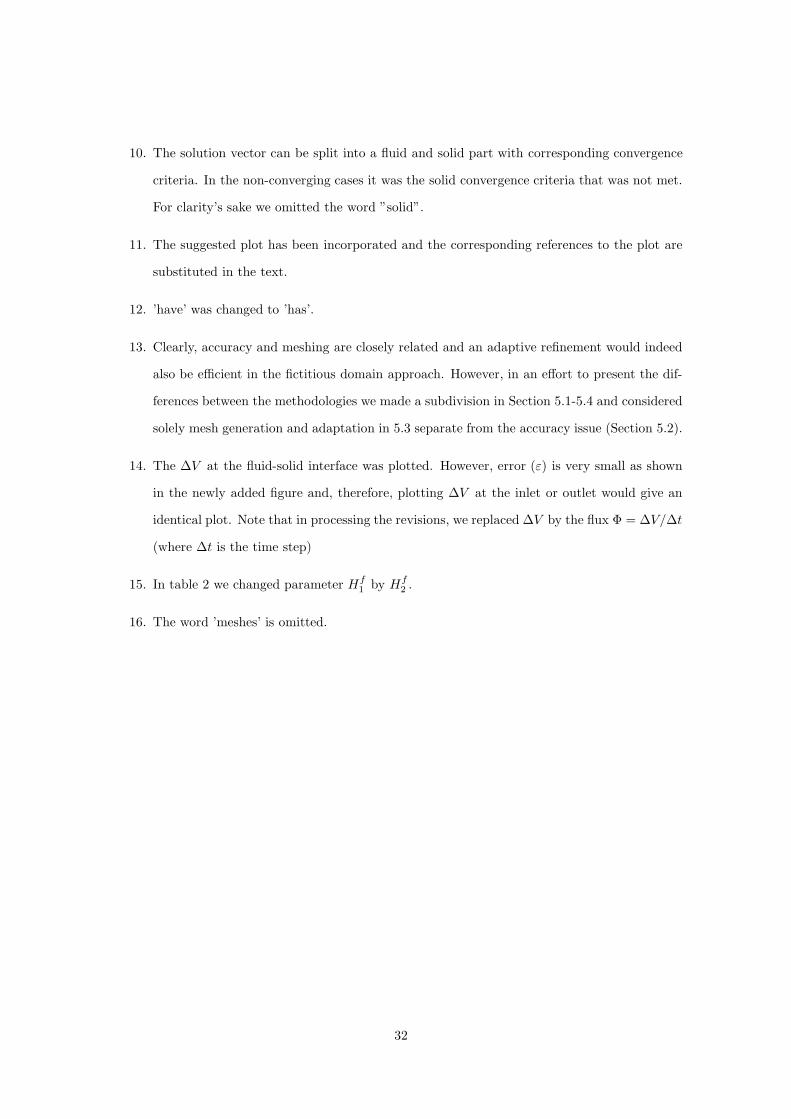
4.2 Self-sustained flapping of a solid slab
The second test case that is considered involves higher flow rates and a less restrained solid body.
The self-sustained flapping of a solid slab has been studied before using numerical codes (Zhu
and Peskin, 2002; Yu, 2005) and is a good test for testing the FSI approaches. A rectangular
fluid domain is considered with a thin solid slab positioned in the middle of the domain that is
aligned in the flow direction (Fig. 9). The corresponding dimensions of the fluid domain and the
solid body are presented in table 1. At the left boundary of the domain a constant velocity with
uniform profile will be prescribed and at the right boundary the fluid flows out freely. A no-slip
condition is applied along the upper and lower boundary. The solid slab was fixed in space at
its left boundary and to initiate the oscillations a disturbance of the alignment of the solid was
introduced by applying an upward boundary force at the first 10 time steps. As shown in Yu
(2005) the amount of disturbance does not influence the final stable state, in which the solid will
oscillate with constant amplitude. The relevant quantities used for the computations are shown
in table 2. The simulation time T was sufficient for the solution to become stable. Note that the
solid was not neutrally-buoyant for this test since inertial effects for the solid are essential for the
self-sustained oscillations to occur (Zhu and Peskin, 2002).
4.2.1 ALE
The material parameters and boundary conditions for this numerical experiment were chosen such
that the displacements of the solid body did not cause the ALE to fail due to collapsed fluid
elements. The mesh shown in Fig. 9 was the coarsest mesh used for the ALE computations. To
prevent ill-shaped elements downstream of the solid the horizontal thin band of fluid elements
attached to the solid tip is prescribed to follow the computed tip displacement in y-direction at
each time step. Since motion of the solid is mainly up and downward we chose to check convergence
by reducing the mesh size only in y-direction and keep the number of solid elements constant. In
table 3 the amplitude is shown for different mesh sizes, where Mesh1 is shown in Fig. 9. For
Mesh2 and Mesh3 the number of fluid elements in y-direction is subsequently doubled. However,
for the ALE computations the refinements did not seem to have a large impact on the amplitude
found. A fine fluid discretisation along the solid boundary to capture the pressure gradients in
that direction seems sufficient to get a spatially converging solution.
12
Page 13
4.2.2 FD/adap
The FD/adap method shows a different behaviour than the ALE approach (Table 3, since lower
values for the amplitude are obtained for the coarser meshes. An explanation for this might be
that the amount of elements above and below the solid changes in time. When the solid is in an
upward position there are only few elements left between the solid and the wall to capture the
pressure gradients that are pushing the leaflet back down. The pressure gradients will be smoothed
over the elements, which will reduce the downward force. Another reason might be that with the
reorientation of the slab toward the vertical direction the discretisation of the adapted interfacial
fluid curve as described in Section 3.2.3 becomes coarser toward the solid tip. Since the coupling
elements are discretised based on this curve, this could result in less accurate coupling near the
solid tip.
4.2.3 FD
Again two coupling approaches for the FD methods are considered. One with coupling points
along the centerline and one with three layers of coupling points across the body. The results
for the computation that used Mesh1, shows the most apparent difference between between both
approaches. While the coupling across the entire body leads to an amplitude of 0.5, coupling along
the centerline results in an amplitude of 0.0. The initial offset does not provide sufficient energy
to initiate the self-sustained oscillations in the case of weaker coupling. Furthermore, we found
that no constant periodic solution was obtained if the fluid mesh was too coarse (Table 3). From
one oscillation to another the amplitude varied by values up to 0.02. However, an increased mesh
resolution solved this problem.
No general trend was found for the convergence and if 0.43 is a converged solution it is not clear
why it is different from the value 0.35 found for the ALE and FD/adap methods. We do, however,
realise that the number of computations performed, was limited. The sensitivity of the FD method
to changes in discretisation and polynomial order of the coupling elements is, therefore, a topic of
interest in the future and should be understood better to make the method more reliable.
5 Discussion
With this work we made an effort to present three different Fictitious Domain approaches that
have been published before and to provide a comparison with an ALE method by means of two
13
Page 14
numerical experiments. It was attempted to lay out the main concerns for the various approaches
in setting up a numerical experiment and additionally to give an impression of their performance.
A short discussion will be given about some important aspects concerning the FSI models.
5.1 Fluid-solid coupling
The ALE method clearly provides the strongest coupling since fluid and solid share nodes at the
solid boundary. Therefore, it can be expected that this method will outperform the FD methods
within the limits of its applicability. A slightly weaker coupling is found for the FD method with
adaptive meshing (FD/adap). However, due to alignment of the fluid and solid mesh at their
interface only interpolation of velocities is required along this interface. In the FD methods any
alignment between the fluid and solid mesh vanishes and the weakest coupling is obtained. The
distribution and amount of points across the solid at which the fluid and solid are coupled has a
large influence on the results. It should be noted that we restricted ourselves to coupling using
a point collocation method. Other choices are possible, like for example the bi-linear coupling
elements used by Yu (2005), that might provide a more robust and accurate coupling.
5.2 Accuracy
Closely related to the fluid-solid coupling is the accuracy of the solution. In general one could say,
the stronger the coupling the more accurate the solutions will be. Both test cases the solutions
show the most accurate results for the ALE approach and the least accurate results for the FD
approach, at a given mesh size. Due to the mesh-alignment at the solid boundary for the ALE
and FD/adap method, a sharp interface defined that divides the fluid domain. In the case of
slender bodies pressure jumps can be captured and the velocity field at one side of the interface
does not interfere with the velocity field at the opposite side. In contrast the fluid elements are
crossed randomly by the solid boundary in the FD methods and although kinematic and dynamic
constraints might hold, that are imposed at the solid boundary, the necessary interpolation will
reduce the accuracy in the vicinity of the boundary. However, depending on the fluid mesh size this
can be a very local phenomenon and the overall flow field can be computed sufficiently accurate.
Furthermore, a reduced accuracy for the fluid velocity does not necessarily influence a correct
computation of the solid motion as demonstrated in Section 4.1.
14
Page 15
5.3 Meshing
The main advantage of the FD method is that mesh generation is only required prior to the com-
putation and that the fluid and solid mesh can be generated separately. Therefore a regular mesh
can be adopted for the fluid mesh. Furthermore, no mesh changes occur during the computation
except for the Lagrangian updating of the solid. With the FD/adap approach a remeshing algo-
rithm is introduced, that adapts the fluid mesh near the boundary of the solid. Since the solid and
fluid mesh do not have to be mutually conforming the algorithm is computationally inexpensive.
However, the meshing algorithm we used is restricted to triangular elements that are less accurate
than their quadrilateral counterparts. And although the method is robust when applied along
smooth boundaries, non-smooth solid boundaries cannot be captured accurately with the current
algorithm. The ALE approach as applied in this study required mutually conforming meshes for
the solid and fluid. Furthermore, the Lagrangian motion of the Eulerian fluid mesh must be com-
puted. The test cases were chosen such that a mesh preserving algorithm was a necessity, which
can become computationally costly depending on the discretisation of the fluid mesh. Note that
the motions of the solid were large but kept within the limits to prevent remeshing.
5.4 Implementation issues
For all methods the fluid and solid matrices are built identically. Beside that, each method has its
own typical requirements. The ALE method has an intrinsic coupling and only requires a routine
to update the fluid mesh after each time step. The FD method requires an extra matrix-build
routine to compute the coupling matrices corresponding to the degrees of freedom that are related
to the Lagrange multiplier. Furthermore, a search routine is required that determines what fluid
element should be used for the interpolation in a coupling point. Finally, the FD/adap method is
probably the most labour intensive since it involves the adaptive meshing algorithm, a matrix-build
routine for the coupling matrices, an element searching routine, an ALE mesh-update routine and
a mapping routine. From this point of view this approach is probably the least favourable.
5.5 General conclusion
Depending on the problem a suitable FSI method should be chosen. The ALE method should
probably be preferred over the other approaches as long as no remeshing is required. The algorithm
is robust, accurate and no extra degrees of freedom are introduced. However, as deformations,
15
Page 16
displacements or rotations of the solid body become larger the FD methods become a sensible
choice. Depending how accurately solutions need to be one could choose to use the FD/adap
approach. Note that the test cases in this study only considered slender bodies, but all approaches
could be used for non-slender 2D or 3D bodies.
5.6 Acknowledgement
The first author is funded by ”Human Resources and Mobility” within the sixth framework pro-
gram by means of a Marie Curie Intra-European Fellowship.
References
F.P.T Baaijens. A fictitious domain/mortar element method for fluid-structure interaction. Int.
J. Num. Meth. Fluids, 35(7):743–761, 2001.
K.J. Bathe. Finite element procedures. Prentice Hall, 1996.
K.J. Bathe and H. Zhang. Finite element develomments for general fluid flows with structural
interactions. Int. J. Num. Meth. Engng., 60:213–232, 2004.
J. De Hart, G.W.M. Peters, P.J.G. Schreurs, and F.P.T Baaijens. A two-dimensional fluid-
structure interaction model of the aortic value. J. Biomech., 33(9):1079–1088, 2000.
J. De Hart, G.W.M. Peters, P.J.G. Schreurs, and F.P.T Baaijens. A three-dimensional compu-
tational analysis of fluid-structure interaction in the aortic valve. J. Biomech., 36(1):103–112,
2003.
R. Dillon and L.J. Fauci. An integrative model of internal axoneme mechanics and external fluid
dynamics in ciliary beating. J. Theor. Biol., 207:415–430, 2000a.
J. Donea, S. Jiuliani, and J.P. Halleux. An arbitrary lagrangian-eulerian finite element method
for transient dynamic fluid-structure interactions. Comp. Meth. Appl. Mech. Eng., 33:689–723,
1982.
A. Gilmanov and F. Sotiropoulos. A hybrid cartesian/immersed boundary method for simulating
flows with 3d, geometrically complex, moving bodies. J. Comp. Phys., 207:457–492, 2005.
16
Page 17
R. Glowinski, T.-W. Pan, and J. Periaux. A lagrange multiplier/fictitious domain method for the
numerical simulation of incompressible viscous flow around moving rigid bodies: (i) case where
the rigid body motions are known a priori. C. R. Acad. Sci. Paris, 25(5):361–369, 1997.
C.W. Hirt, A.A. Amsden, and J.L. Cook. An arbitrary lagrangian-eulerian computing method for
all speeds. J. Comp. Phys., 14:227–253, 1974.
T.J.R. Hughes, W.K. Liu, and T. Zimmerman. Lagrangian-eulerian finite element formulation for
incompressible viscous flow. Comp. Meth. Appl. Mech. Eng., 29:329–349, 1981.
C.S. Peskin. The immersed boundary method. Acta Numerica, 11:479–517, 2002.
C.S. Peskin. Flow patterns around heart valves: a numerical method. J. Comp. Phys., 10:252–271,
1972.
C.S. Peskin and D.M. McQueen. A three-dimensional computational method for blood flow in the
heart i. immersed elastic fibers in a viscous incompressible fluid. J. Comp. Phys., 81:372–405,
1989.
A. Segal. SEPRAN Introduction, User’s Manual, Programmer’s Guide, Standard Problems. Inge-
nieursbureau SEPRA, Leidschendam, 2003.
R. Van Loon, P.D. Anderson, J. De Hart, and F.P.T. Baaijens. A combined fictitious do-
main/adaptive meshing method for fluid-structure interaction in heart valves. Int. J. Num.
Meth. Fluids, 46:533–544, 2004.
R. Van Loon, P.D. Anderson, and F.N. Van de Vosse. A fluid-structure interaction method with
solid-rigid contact for heart valve dynamics. J. Comp. Phys., Accept., 2006.
X. Wang and W.K. Liu. Extended immersed boundary method using fem and rkpm. Comput.
Meth. Appl. Mech. Engrg., 193:1305–1321, 2004.
Z. Yu. A DLM/FD method for fluid/flexible-body interactions. J. Comp. Phys., 207:1–27, 2005.
L. Zhang, A. Gerstenberger, X. Wang, and W.K. Liu. Immersed finite element method. Comput.
Meth. Appl. Mech. Engrg., 193:2015–2067, 2004.
L. Zhu and C.S. Peskin. Simulation of a flapping flexible filament in a flowing soap film by the
immersed boundary method. J. Comp. Phys., 179:452–468, 2002.
17
Page 18
Figure 1: The mesh computed for the ALE computations consists of shared fluid-solid nodes. This
ensures a strong coupling in the FSI.
18
Page 19
2
34
1
(a)
3
4
1
2
(b)
1
4
3
2
(c)
Figure 2: Schematic representation of an ALE (b), and fictitious domain (c) method. Starting
from (a) rotation of the solid gray body leads to (b) or (c) depending on the method used.
19
Page 20
(a) (b)
Figure 3: The quadrilateral solid mesh is coupled to the triangular fluid mesh in collocation points
(denoted by ©) using the solid discretisation. Plot (a) shows the discretisation along the centerline
curve of the solid and plot (b) shows the collocation points for coupling across the entire body.
20
Page 21
(a) (b)
Figure 4: Plot (a) shows the non-conforming meshes for the fluid and structure in the FD/adap
approach. Along the interface the coupling elements will have the same discretisation as the fluid
as shown in plot (b).
21
Page 22
f2f2f1
f3
Figure 5: Fluid induced deformations of a membrane (dashed lines) at several time points.
22
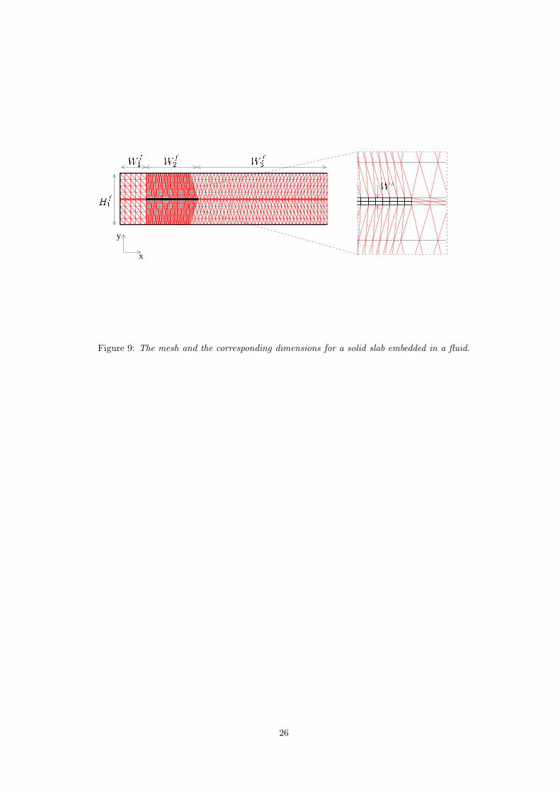
Page 23
W f1 W f2
W f3
W s
W f2Hf1
Hf2P
Figure 6: The mesh and the corresponding dimensions for a membrane embedded in a fluid.
23
Page 24
0 0.2 0.4 0.6 0.8 1 1.2 1.4 1.6 1.8−1
−0.5
0
0.5
1
1.5
2
2.5
ALE
FD
FD/adap
t[s]
Φm
em
[cm
2/s
]
Figure 7: Fluid flux Φmem measured at the membrane interface as a function of time. A comparison
between the ALE, FD and FD/adap method using the fluid mesh of Fig. 6. Note that a solid mesh
of 150x4 was required for the FD method compared to 50x4 for both other approaches.
24
Page 25
0 0.2 0.4 0.6 0.8 1 1.2 1.4 1.6 1.8
−3
−2.5
−2
−1.5
−1
−0.5
0
0.5x 10
−4
ALE
FD
FD/adap
time
ε
Figure 8: The relative error ε in fluid flux at the membrane interface compared to the inlet flux
with ε = (Φmem(t) − Φin(t))/ max (Φin).
25
Page 26
x
y
Hf1 W sW f3W f1 W f2
Figure 9: The mesh and the corresponding dimensions for a solid slab embedded in a fluid.
26
Page 27
Table 1: Relevant geometric parameter values
W f1 (cm) W f
2 (cm) W f3 (cm) Hf
1 (cm) Hf2 (cm) Ws(cm)
Num. Exp. 4.1 1.0 0.5 2.0 0.5 1.0 0.016
Num. Exp. 4.2 1.0 2.0 5.0 2.0 − 0.05
27
Page 28
Table 2: Relevant parameter values for the numerical experiments.
umax (m/s) pmax (Pa) η (Pa s) ρf (kg/m3) ρs (kg/m3) T (s) G (MPa)
Num. Exp. 4.1 − 8.0 4.0 × 10⁻³ 103 103 2.0 100
Num. Exp. 4.2 20.0 − 4.0 × 10⁻³ 103 11 · 103 2.0 50
28
Page 29
Table 3: Amplitudes of oscillations for different mesh sizes. (∗ non-constant amplitude)
Mesh1 Mesh2 Mesh3 Mesh4
ALE 0.36 0.35 0.35 -
FD/adap 0.27 0.33 0.35 -
FD (body) 0.5∗ 0.42 0.43 0.35
FD (line) damps 0.43∗ 0.30 -
29
Page 30
Reviewer 1
1. We disagree that the Crouzeix-Raviart elements used in this paper do not satisfy the lo-
cal conservation of flux. Since the weight functions related to the continuity equation and
corresponding pressure variables are discontinuous for these types of elements, mass conser-
vation is enforced over the element (see: Fortin, Int. J. Num. Meth. Fluids, 1981). We do
acknowledge that the elements described in Bathe’s 2002 paper enforce a local conservation
of momentum, where the Crouzeix-Raviart elements do not, but we do not think that this
introduces substantial errors in the test cases considered.
2. Using a solid material law is indeed not the most efficient way to update the fluid mesh.
Although we did not encounter any stability issues for the test problems presented, we
recognise that solving a Laplace problem is more efficient, robust and therefore widely used.
It is also no necessity to use a conforming fluid-solid interface as clearly illustrated in the
reference papers mentioned. However, our main interest was the functionality/accuracy of
the fictitious domain approaches. The ALE problem was set up to provide a reference state.
We incorporated the references mentioned by the reviewer and added the here described
comments on in Section 3.2.1.
3. The reference to the book has been incorporated in Sectionn 3.2 on page 6.
4. ALE methods have been extensively and succesfully used for fluid-structure interaction prob-
lems in 2D as well as 3D. The method proposed by Baaijens (see reference list) has been
implemented in 3D and used for aortic heart valve models by De Hart (see reference list).
The 3D code is validated using reduced 2D experimental models considering a rigid valve
[Stijnen et al., J. Fluid and Struct., 2004]. Finally, the fictitious domain approach combined
with adaptive meshing has also been published in 3D [Van Loon et al., C.R. Mecanique,
2005] including a comparison of full 3D and axisymmetric 3D finite element models. In
conclusion, we can say that each of the methods has been extended to three dimensions,
although their performance has not been tested extensively.
5. Several typos have been removed and we rephrased some sentences.
30
Page 31
Reviewer 2
The variational formulation Eqs (10)-(12) does indeed not incorporate the terms related to the
stresses of the fluid in the solid domain. In the first paragraph of page 4 we shortly mention that
this term was neglected in our models. Reason for this is that the elastic forces will dominate the
fluid forces in this domain. A same reasoning can be found in and Zhang/2004 and Yu/2005 (see
reference list).
For sake of clarity we have altered the formulation incorporating the stress term, which is then
complete. Thereafter an explanation is given for neglecting the term in the implementation in the
first paragraph on page 6. In addition we incorporated some of the references mentioned by the
reviewer in our introduction.
Reviewer 3
1. Changed accordingly.
2. Indeed stress equilibrium at the fluid-solid interface should be added as an extra constraint.
For the ALE formulation used in this work this requirement is fulfilled automatically by tak-
ing conforming meshes and solving the coupled system implicitly. For the fictitious domain
methods the introduced Lagrange multiplier represents the traction forces between the fluid
and the solid, which ensures the stresses to be in balance. We added the constraint to the
governing equations on page 5.
3. We included a reference to SEPRAN.
4. We agree that an ALE method does not restrict one to conforming meshes. In the ALE
approach presented, however, we did restrict ourselves to conforming meshes. We made
adjustments in section 3.2.2 to clarify that ALE is not restricted to conforming meshes.
5. We removed the second ”will”.
6. We removed the brackets.
7. We defined the boundary conditions in a less ambiguous manner.
8. We changed the indexes.
9. We took the maximum Φin as a fixed reference to compute the relative error.
31
Page 32
10. The solution vector can be split into a fluid and solid part with corresponding convergence
criteria. In the non-converging cases it was the solid convergence criteria that was not met.
For clarity’s sake we omitted the word ”solid”.
11. The suggested plot has been incorporated and the corresponding references to the plot are
substituted in the text.
12. ’have’ was changed to ’has’.
13. Clearly, accuracy and meshing are closely related and an adaptive refinement would indeed
also be efficient in the fictitious domain approach. However, in an effort to present the dif-
ferences between the methodologies we made a subdivision in Section 5.1-5.4 and considered
solely mesh generation and adaptation in 5.3 separate from the accuracy issue (Section 5.2).
14. The ∆V at the fluid-solid interface was plotted. However, error (ε) is very small as shown
in the newly added figure and, therefore, plotting ∆V at the inlet or outlet would give an
identical plot. Note that in processing the revisions, we replaced ∆V by the flux Φ = ∆V/∆t
(where ∆t is the time step)
15. In table 2 we changed parameter Hf1 by Hf
2 .
16. The word ’meshes’ is omitted.
32