COMPENDIUM OF CLAIMS AND PROOFS, PART I CARLOS PASQUALI Contents 1. The Star Product 1 1.1. Properties of the Diamond Operator 2 1.2. Properties of the J Transformation 3 1.3. Properties of the Star Operator 3 1.4. Mechanics of Powering 6 2. Pasquali Patches 6 2.1. Definitions and Constructions 6 2.2. Properties of Pasquali Patches Under the Star Operator 7 2.3. Limiting Surface 9 2.4. Probability Distribution Transformations via Pasquali Patches 11 2.5. Fixed Distribution Conjecture 11 2.6. Fixed Distribution Existence 14 2.7. Probability Distribution Transformations via Pasquali Patch Power Collections 16 2.8. Dynamics 19 3. Relevant Generalizations 19 3.1. Specific Finite-Sum Surface Eigenvalues 19 3.2. Functions on Eigenvalues of Specific Finite-Sum Surfaces 23 4. Equivalencies of the Star Operator 24 5. Other Claims and Proofs 24 6. Proofs in Progress 24 1. The Star Product Definition 1.1 (The Star Operator). (October 17, 2010, January 17, 2013) • On Two Surfaces Let f (x, y) and g(x, y) be surfaces so that f,g : [0, 1] × [0, 1] → R. The star operator ? : [0, 1] 2 × [0, 1] 2 → [0, 1] 2 takes two surfaces and creates another in the following way: (f (x, y),g(x, y)) (f (1 - y,z),g(x, y)) h(x, z) h(x, y) with the central transformation being defined by : [0, 1] 2 × [0, 1] 2 → [0, 1] 2 f (1 - y,z) g(x, y)= Z 1 0 f (1 - y,z)g(x, y) dy = h(x, z) and the last transformation that takes h(x, z) h(x, y) we will call j : [0, 1] 2 → [0, 1] 2 . Thus f (x, y) ?g(x, y)= j (f (1 - y,z) g(x, y)) = j Z 1 0 f (1 - y,z)g(x, y) dy In the special case where f (x, 0), we have f (1 - y, 0) g(x, y)= Z 1 0 f (1 - y, 0)g(x, y) dy = h(x, 0) 1
Transcript
COMPENDIUM OF CLAIMS AND PROOFS, PART I
CARLOS PASQUALI
Contents
1. The Star Product 1
1.1. Properties of the Diamond Operator 21.2. Properties of the J Transformation 3
1.3. Properties of the Star Operator 3
1.4. Mechanics of Powering 62. Pasquali Patches 6
2.1. Definitions and Constructions 6
2.2. Properties of Pasquali Patches Under the Star Operator 72.3. Limiting Surface 9
2.4. Probability Distribution Transformations via Pasquali Patches 11
2.5. Fixed Distribution Conjecture 112.6. Fixed Distribution Existence 14
2.7. Probability Distribution Transformations via Pasquali Patch Power Collections 162.8. Dynamics 19
3. Relevant Generalizations 19
3.1. Specific Finite-Sum Surface Eigenvalues 193.2. Functions on Eigenvalues of Specific Finite-Sum Surfaces 23
4. Equivalencies of the Star Operator 24
5. Other Claims and Proofs 246. Proofs in Progress 24
1. The Star Product
Definition 1.1 (The Star Operator). (October 17, 2010, January 17, 2013)
• On Two Surfaces
Let f(x, y) and g(x, y) be surfaces so that f, g : [0, 1] × [0, 1] → R. The star operator ? : [0, 1]2 × [0, 1]2 → [0, 1]2
takes two surfaces and creates another in the following way:
with the central transformation being defined by � : [0, 1]2 × [0, 1]2 → [0, 1]2
f(1− y, z) � g(x, y) =
∫ 1
0f(1− y, z)g(x, y) dy = h(x, z)
and the last transformation that takes h(x, z) h(x, y) we will call j : [0, 1]2 → [0, 1]2. Thus
f(x, y) ? g(x, y) = j (f(1− y, z) � g(x, y)) = j
(∫ 1
0f(1− y, z)g(x, y) dy
)In the special case where f(x, 0), we have
f(1− y, 0) � g(x, y) =
∫ 1
0f(1− y, 0)g(x, y) dy = h(x, 0)
1
2 CARLOS PASQUALI
motivating the following simplification:
• On a Function and a Surface
Let f(x) be a function f : [0, 1]→ R, and g(x, y) a function such that g : [0, 1]2 → R. The star operator ? : [0, 1]×[0, 1]2 → [0, 1] takes the function and the surface and creates another function in the following way:
(f(x), g(x, y)) (f(1− y), g(x, y)) h(x)
with the last transformation being defined by � : [0, 1]× [0, 1]2 → [0, 1]
f(1− y) � g(x, y) =
∫ 1
0f(1− y)g(x, y)dy = h(x)
Thus we have
f(x) ? g(x, y) = f(1− y) � g(x, y) =
∫ 1
0f(1− y)g(x, y) dy
1.1. Properties of the Diamond Operator.
1.1.1. Linearity.
Claim 1.1. (January 29, 2013) The diamond operator is a linear operator.
Proof Linearity follows from the integral operator properties. Thus we have:
• Surface diamond Surface
Letting f, g, h : [0, 1]2 → R, and c be a constant,
(c · f) � g =
∫ 1
0(c · f(x, y)) g(x, y) dy
= c
∫ 1
0f(x, y)g(x, y) dy
= c · (f � g)
f � (c · g) =
∫ 1
0f(x, y) (c · g(x, y)) dy
= c
∫ 1
0f(x, y)g(x, y) dy
= c · (f � g)and
(f + g) � h =
∫ 1
0(f(x, y) + g(x, y))h(x, y) dy
=
∫ 1
0f(x, y)h(x, y) dy +
∫ 1
0g(x, y)h(x, y) dy
= f � h+ g � h
f � (g + h) =
∫ 1
0f(x, y) (g(x, y) + h(x, y)) dy
=
∫ 1
0f(x, y)g(x, y) dy +
∫ 1
0f(x, y)h(x, y) dy
= f � g + f � h• Function diamond Surface
Letting d, e : [0, 1]→ R and f, g : [0, 1]2 → R, and c be a constant,
(c · d) � f =
∫ 1
0(c · d(x)) f(x, y) dy
= c
∫ 1
0d(x)f(x, y) dy
= c · (d � f)
COMPENDIUM OF CLAIMS AND PROOFS, PART I 3
d � (c · f) =
∫ 1
0d(x) (c · f(x, y)) dy
= c
∫ 1
0d(x)f(x, y) dy
= c · (d � f)
and
(d+ e) � f =
∫ 1
0(d(x) + e(x)) f(x, y) dy
=
∫ 1
0d(x)f(x, y) dy +
∫ 1
0e(x)f(x, y) dy
= d � f + e � f
d � (f + g) =
∫ 1
0d(x) (f(x, y) + g(x, y)) dy
=
∫ 1
0d(x)f(x, y) dy +
∫ 1
0d(x)g(x, y) dy
= d � f + d � g
�
1.2. Properties of the J Transformation.
1.2.1. Linearity.
Claim 1.2. (January 29, 2013) The transformation j : [0, 1]2 → [0, 1]2 is likewise linear.
Proof Let f, g : [0, 1]2 → R, and c be a constant. Then:
j (c · f(x, z)) = c · f(x, y)
= c · j (f(x, z))
Also:
j (f(x, z) + g(x, z)) = f(x, y) + g(x, y)
= j (f(x, z)) + j (g(x, z))
�
1.2.2. Other Properties.
Claim 1.3. (January 17, 2013) Take the transformation j : [0, 1]2 → [0, 1]2 that carries h(x, z) h(x, y). Then:∫ b
aj(h(x, z)) dx = j
(∫ b
ah(x, z) dx
)Proof ∫ b
aj(h(x, z)) dx =
∫ b
ah(x, y) dx = H(0, y)
On the other hand
j
(∫ b
ah(x, z) dx
)= j (H(0, z)) = H(0, y)
�
1.3. Properties of the Star Operator.
4 CARLOS PASQUALI
1.3.1. Linearity.
Corollary 1.4 (Scaling of the Star Product). (January 30, 2013)Let d(x) be a function e : [0, 1]→ R, and f(x, y) and g(x, y) be functions f, g : [0, 1]2 → R, c is a constant. Then:
• Surface star Surface
(c · f) ? g = c · (f ? g)and
f ? (c · g) = c · (f ? g)• Function star Surface
(c · d) ? f = c · (d ? f)
and
d ? (c · f) = c · (d ? f)
Proof This is a consequence of Claim 1.1 and Claim 1.2.
• Surface star Surface
(c · f) ? g = j ((c · f(1− y, z)) � g(x, y))
= c · j (f(1− y, z) � g(x, y))
= c · (f ? g)and
f ? (c · g) = j (f(1− y, z) � (c · g(x, y)))
= c · j (f(1− y, z) � g(x, y))
= c · (f ? g)• Function star Surface
(c · d) ? f = j ((c · d(1− y)) � f(x, y))
= c · j (d(1− y) � f(x, y))
= c · (d ? f)
andd ? (c · f) = j (d(1− y) � (c · f(x, y)))
= c · j (d(1− y) � f(x, y))
= c · (d ? f)
�
Corollary 1.5 (Distributive Property of the Star Product). (January 27, 2013)Let d(x), e(x) be a functions d, e : [0, 1]→ R and f(x, y), g(x, y) and h(x, y) be functions f, g, h : [0, 1]2 → R, c is
a constant. Then:
• Surface star Surface
(f + g) ? h = f ? h+ g ? h
and
f ? (g + h) = f ? g + f ? h
• Function star Surface
(d+ e) ? f = d ? f + e ? f
and
d ? (f + g) = d ? f + d ? g
Proof Again this is a consequence of Claim 1.1 and Claim 1.2.
• Surface star Surface
COMPENDIUM OF CLAIMS AND PROOFS, PART I 5
We have:(f + g) ? h = j ((f(1− y, z) + g(1− y, z)) � h(x, y))
= j (f(1− y, z) � h(x, y) + g(1− y, z) � h(x, y))
= j (f(1− y, z) � h(x, y)) + j (g(1− y, z) � h(x, y))
= f ? h+ g ? h
The second to last line is again a consequence of Claim 1.2.
The second part is:f ? (g + h) = j (f(1− y, z) � (g(x, y) + h(x, y)))
= j (f(1− y, z) � g(x, y) + f(1− y, z) � h(x, y))
= j (f(1− y, z) � g(x, y)) + j (f(1− y, z) � h(x, y))
= f ? g + f ? h
where the second to last line is justified by Claim 1.2.
• Function star Surface
Rewriting the first part,(d+ e) ? f = (d(1− y) + e(1− y)) � f(x, y)
= d(1− y) � f(x, y) + e(1− y) � f(x, y)
= d ? f + e ? f
follows directly from the linear properties of the diamond operator Claim 1.1.Next, in the second part,
d ? (f + g) = d(1− y) � (f(x, y) + g(x, y))
= d(1− y) � f(x, y) + d(1− y) � g(x, y)
= d ? f + d ? g
again by Claim 1.1. �
1.3.2. Other Properties.
Claim 1.6 (Non-commutativity). (October 17, 2010) The star product is non-commutative.
Proof by Counterexample The claim only makes sense from the viewpoint of surfaces.
• On Surfaces
Let f, g : [0, 1]2 → R.
We want to show that f(x, y) ? g(x, y) 6= g(x, y) ? f(x, y). Choose f(x, y) = x and g(x, y) = y without loss of
generality. Then:
f(x, y) ? g(x, y) = f(x) ? g(x, y) =
∫ 1
0f(1− y) · g(x, y) dy =
∫ 1
0(1− y) · y dy =
∫ 1
0
(y − y2
)dy =
1
6
and
g(x, y) ? f(x, y) = j
(∫ 1
0g(1− y, z) · f(x, y) dy
)= j
(∫ 1
0(z · x) dy
)= j (z · x) = y · x
are non-equal. �
Claim 1.7 (Associativity). (October 17, 2010) The star product is associative.
Proof Again the claim only makes sense for the star operator on surfaces.
• On Surfaces
Let f, g, h : [0, 1]2 → R.
We want to show that [f(x, y) ? g(x, y)] ? h(x, y) = f(x, y) ? [g(x, y) ? h(x, y)].The LHS is:
[f(x, y) ? g(x, y)] ? h(x, y) = j
(∫ 1
0f(1− y, z)g(x, y) dy
)? h(x, y)
= j
(∫ 1
0
∫ 1
0f(1− z, w)g(1− y, z) dz h(x, y) dy
)
6 CARLOS PASQUALI
= j
(∫ 1
0
∫ 1
0f(1− z, w)g(1− y, z)h(x, y) dz dy
)The RHS is:
f(x, y) ? [g(x, y) ? h(x, y)] = f(x, y) ? j
(∫ 1
0g(1− y, z)h(x, y) dy
)= j
(∫ 1
0f(1− z, w)
∫ 1
0g(1− y, z)h(x, y) dy dz
)= j
(∫ 1
0
∫ 1
0f(1− z, w)g(1− y, z)h(x, y) dy dz
)We immediately see the equivalence using the Fubini Theorem to exchange the order of integration. �
1.4. Mechanics of Powering.
Claim 1.8 (Powering Symmetry). (December 30, 2012) Take f : [0, 1]2 → R. Let the nth power of f(x, y), fn(x, y)
be denoted shorthand by Fn (for Pasquali patches, we use the notation Pn and pn(x, y) interchangeably). Then form,n ≥ 1, Fn ? Fm = Fm ? Fn.
Proof by Induction By definition of powering,
F 1 ? Fm = F 1 ? (F 1 ? . . . ? F 1)︸ ︷︷ ︸m times
Then, by Claim 1.7 Associativity of the Star Product, this is equivalent to
(F 1 ? . . . ? F 1)︸ ︷︷ ︸m times
?F 1 = Fm ? F 1
Next assume that, for fixed k,m ≥ 1, Fk ? Fm = Fm ? Fk.
Then Fk+1 ?Fm = (F 1 ?Fk)?Fm, where this bit we take as the definition of powering, and then, by Claim 1.7again, F 1 ? (Fk ? Fm), which then by our inductive hypothesis equals F 1 ? (Fm ? Fk) and this is (Fm ? Fk) ? F 1
by the inductive basis. Again, Claim 1.7 gives Fm ? (Fk ? F 1) and lastly Fm ? F 1+k by definition of powering.
Axiomatic commutativity of the positive integers gives Fm ? Fk+1 and we are done.By symmetry of equality itself, we need only do a single proof of induction on one of the power parameters. �
Claim 1.9. (December 30, 2012) Again take f : [0, 1]2 → R. Fn ? Fm = Fm+n.
Proof by Induction First, fix m ≥ 1. By the definition of powering, F 1 ? Fm = Fm+1. Next, suppose it’s true
that Fk ? Fm = Fm+k. Then Fk+1 ? Fm equals (F 1 ? Fk) ? Fm by definition of powering, and by Claim 1.7
Associativity of the Star Product we get F 1 ? (Fk ? Fm) or F 1 ? Fm+k using the inductive hypothesis. By the
inductive basis, this becomes F (m+k)+1, that is Fm+(k+1) using associativity of the positive integers, which we take
as axiomatic.
Having done so, next fix n ≥ 1 and let m vary. We have Fn?F 1 = F 1?Fn by Claim 1.8 Powering Symmetry.Since this part of the proof is identical to the one we just wrote, we are done. �
2. Pasquali Patches
2.1. Definitions and Constructions.
Definition 2.1 (Pasquali patch). (April 22, 2010) Define a continuous surface p(x, y), with p : [0, 1] × [0, 1] →R+ ∪{0}, and let
∫ 10 p(x, y) dx = 1 be true regardless of the value of y. In other words, integrating such surface with
respect to x yields the uniform probability distribution u(y), u : [0, 1]→ {1}. We will call this a Pasquali patch.
Construction 2.1. (October 10, 2010) A way to construct a Pasquali patch is by positing
p(x, y) = f1(x)g1(y) + f2(x)1− g1(y)
∫ 10 f1(x) dx∫ 1
0 f2(x) dx= f1(x)g1(y) + f2(x)
1− g1(y)F1
F2
for arbitrary function choices f1,2(x), and g1(y).
COMPENDIUM OF CLAIMS AND PROOFS, PART I 7
Proof Since for Pasquali patches∫ 10 p(x, y) dx = 1, it can be seen that such construction is a Pasquali patch because∫ 1
0
(f1(x)g1(y) + f2(x)
1− g1(y)F1
F2
)dx = g1(y)F1 +
F2
F2−g1(y)F1F2
F2= 1
regardless of function choices of y. �
2.2. Properties of Pasquali Patches Under the Star Operator.
2.2.1. Notable Properties.
Claim 2.1 (Closure of Pasquali Patches). (October 12, 2010) A Pasquali patch star a Pasquali patch yields anew Pasquali patch. In particular, a Pasquali patch star itself ( Pasquali patch powers) will always yield another
Pasquali patch.
Proof Take Pasquali patches p(x, y) and q(x, y). We want to show that p(x, y)?q(x, y) = r(x, y) is a Pasquali patch.
Thus, we want to show that∫ 10 r(x, y) dx = 1. In other words,∫ 1
0j
(∫ 1
0p(1− y, z)q(x, y) dy
)dx = 1
By Claim 1.3, we can write this as
j
(∫ 1
0
∫ 1
0p(1− y, z)q(x, y) dy dx
)We can exchange the order of integration because of absolute convergence of the integrals (Fubini Theorem). Thus
j
(∫ 1
0p(1− y, z)
∫ 1
0q(x, y) dx dy
)yields
j
(∫ 1
0p(1− y, z)u(y) dy
)= j
(∫ 1
0p(1− y, z) dy
)This final integral evaluates to j (u(z)) = u(y) = 1 for any choice of y. Thus
∫ 10 r(x, y) dx = 1. �
Example 2.1. (October 12, 2010) Take the Pasquali patch p(x, y) = x2y3 + x(
2− 2y3
3
). It is evident it is a
Pasquali patch because ∫ 1
0
[x2y3 + x
(2−
2y3
3
)]dx =
[x3
3y3 +
x2
2
(2−
2y3
3
)]∣∣∣∣10
= 1
We can calculate
p(1− y, z) = z3y2 −4z3y
3+z3
3− 2y + 2
so that the second “power” of the Pasquali patch is
p2(x, y) = j
(∫ 1
0p(1− y, z)p(x, y) dy
)= j
(29x
15+z3x
90+x2
10−z3x2
60
)and the final transformation j of the star operator gives
p2(x, y) =29x
15+y3x
90+x2
10−y3x2
60
One easily checks p2(x, y) is indeed a Pasquali patch by performing the integral∫ 10 p2(x, y) dx and ascertaining its
equality to 1. The third Pasquali patch power is
p3(x, y) =1741x
900−
y3x
5400+
59x2
600+y3x2
3600
Example 2.2. (October 15, 2010, October 17, 2010) The Pasquali patch
p(x, y) = 1− cos(2πx) cos(2πy)
has powers:
p(x, y) = 1− cos(2πx) cos(2πy)
p2(x, y) = 1 +cos(2πx) cos(2πy)
2
8 CARLOS PASQUALI
p3(x, y) = 1−cos(2πx) cos(2πy)
4
p4(x, y) = 1 +cos(2πx) cos(2πy)
8
p5(x, y) = 1−cos(2πx) cos(2πy)
16
p6(x, y) = 1 +cos(2πx) cos(2πy)
32
...
pn(x, y) = 1−cos(2πx) cos(2πy)
(−2)(n−1)
Proof by Induction We show that, by the inductive basis, p(x, y) = 1− cos(2πx) cos(2πy) must equal
p1(x, y) = 1−cos(2πx) cos(2πy)
(−2)(0)
which a quick check shows is indeed the case.
Next, by the inductive step, we take as true that:
pk(x, y) = 1−cos(2πx) cos(2πy)
(−2)(k−1)
Then,
pk+1(x, y) = j
(∫ 1
0p1(1− y, z) · pk(x, y) dy
)= j
(∫ 1
0(1− cos(2π(1− y)) cos(2πz)) ·
(1−
cos(2πx) cos(2πy)
(−2)k−1
)dy
)The product of 1 with itself is 1, and such will integrate to 1 in the unit interval. So we save it. The integrals∫ 1
0 cos(2πy) dy and∫ 10 cos(2π − 2πy) dy both evaluate to zero, so we are left only with the task of evaluating the
crossterm:∫ 1
0cos(2π(1− y)) cos(2πz) ·
cos(2πx) cos(2πy)
(−2)k−1dy =
cos(2πz) cos(2πx)
(−2)k−1
∫ 1
0cos(2π − 2πy) cos(2πy) dy
=cos(2πz) cos(2πx)
(−2)k−1
∫ 1
0cos2(2πy) dy
=cos(2πz) cos(2πx)
(−2)k−1·
1
2
= −cos(2πz) cos(2πx)
(−2)k
Let’s not forget the 1 we had saved, so:
pk+1(x, y) = j
(1−
cos(2πx) cos(2πz)
(−2)k
)= 1−
cos(2πx) cos(2πy)
(−2)k
as we wanted to show. �
Remark 2.1. (April 22, 2010) Probabilistic Interpretation. In direct analogy to the Chapman-Kolmogorovequation, transition from state y ∈ [0, 1] to x ∈ [0, 1] in n + m steps can be achieved by first transitioning to an
intermediate state x• in n steps and then jumping from there to x in m more steps. Particularly, all states areachievable from a starter state since for Pasquali patch p(x, y) there are only a finite number of zeroes in the domain
because the surface is well-behaved.
COMPENDIUM OF CLAIMS AND PROOFS, PART I 9
2.2.2. Other Properties.
Claim 2.2 (Non-commutativity of Pasquali Patches Under the Star Product). (October 17, 2010) We know in
general the star product is non-commutative (Claim 1.6), but we don’t know that Pasquali patches as a subset of
surfaces with domain on [0, 1]× [0, 1] (“ Pasquali patchixes”, due to their resembling matrixes in that they transformfunctions to other functions, as matrixes transform vectors to other vectors) don’t commute.
Proof by Counterexample Suppose the Pasquali patches p(x, y) = x+ 12
and q(x, y) = 1 + xy − y2
. Then
p(x, y) ? q(x, y) = p(x) ? q(x, y) =
∫ 1
0p(1− y) · q(x, y) dy
=
∫ 1
0
(3
2− y)·(
1 + xy −y
2
)dy
=5x
12+
19
24
where
q(x, y) ? p(x, y) = j
(∫ 1
0q(1− y, z) · p(x, y) dy
)= j
(∫ 1
0q(1− y, z) · p(x) dy
)= j
(p(x)
∫ 1
0q(1− y, z) dy
)= j (p(x) · u(z)) = p(x)
= x+1
2�
Corollary 2.3 (Associativity of Pasquali Patches Under the Star Product). (October 17, 2010, December 3,2012) Pasquali patches inherit associativity.
Proof Pasquali patches inherit associativity from the star product through Claim 1.7 Associativity of the Star
Product. �
2.3. Limiting Surface.
Definition 2.2. The limiting, steady-state, or stationary surface is a surface obtained by taking the limit as n
approaches infinity of Pasquali patch powers limn→∞ pn(x, y), provided it exists, and we call it p∞(x, y).
Lemma 2.4. (October 17, 2010) The stationary surface of
p(x, y) = 1− cos(2πx) cos(2πy)
is p∞(x, y) = 1.
Proof Since the Pasquali patch power collection of p(x, y) = 1− cos(2πx) cos(2πy) can be described by
pn(x, y) = 1−cos(2πx) cos(2πy)
(−2)(n−1)
due to Example 2.2 we need only take the limit as n approaches infinity of this formula:
limn→∞
pn(x, y) = limn→∞
(1−
cos(2πx) cos(2πy)
(−2)(n−1)
)= 1
In this particular case, notice that p∞(x, y) = 1 is also a Pasquali patch because∫ 1
0p∞(x, y) dx = 1
�
Lemma 2.5. (December 3, 2012) If the sequence pn(x, y) of Pasquali patch powers converge uniformly to p∞(x, y),
then p∞(x, y) is a Pasquali patch.
10 CARLOS PASQUALI
Proof We want to show that∫ 10 p∞(x, y) dx = 1. First,∫ 1
0p∞(x, y) dx =
∫ 1
0limn→∞
pn(x, y) dx
By uniform convergence of the sequence of Pasquali patches, we can exchange the order of the limit to obtain
limn→∞
∫ 1
0pn(x, y) dx
Now for any n, pn(x, y) is a Pasquali patch, and therefore the integral is equal to 1 in every case (for any choice ofn). Lastly,
limn→∞
{1}n = 1
and we have arrived at what we wanted to show. �
Claim 2.6. (December 3, 2012) Pasquali patches that are functions of y (possibly x) explicitly generate by self-powering a countably infinite collection of Pasquali patches that are functions of y (possibly x) explicitly.
Proof by Induction Let p(x, y) be a Pasquali patch that is a function of y (possibly x) explicitly. Thus the basisis true by hypothesis. By the inductive step, let pk(x, y), k ∈ Z+ be an explicit function of y (possibly x). Then:
pk+1(x, y) = pk(x, y) ? p(x, y) = j
(∫ 1
0pk(1− y, z)p(x, y) dy
)is an explicit function of y (possibly x) since pk(x, y) was an explicit function of y (possibly x), and the y was savedby the transformation to z in pk(1 − y, z), so that the integral did not aggregate it. Then, the transformation j
takes z y makes pk+1(x, y) an explicit function of y (possibly x). The result is a countable collection of explicit
functions of y (possibly x) via self-powering, because k ∈ Z+. �
Claim 2.7. (October 17, 2010) A Pasquali patch star a Pasquali patch that is solely a function of x returns thesecond Pasquali patch.
Proof Suppose the Pasquali patches q(x, y) and p(x, y) = p(x). Then:
q(x, y) ? p(x, y) = j
(∫ 1
0q(1− y, z) · p(x) dy
)= j
(p(x)
∫ 1
0q(1− y, z) dy
)= j (p(x) · u(z)) = p(x)
�
Claim 2.8. (December 3, 2012) Pasquali patches that are functions of x alone (explicitly or otherwise) generate
Pasquali patches that are the same as the original Pasquali patch via self-powering.
Proof by Induction p(x) = p(x) by the identity of equality. p2(x) = p(x) ? p(x) = p(x) by Claim 2.7. This
establishes the induction basis. Next, suppose pk(x) = p(x). Then pk+1(x) = pk(x) ? p(x) = p(x) ? p(x) = p(x), andwe are done. �
Claim 2.9. (December 3, 2012) If the limiting surface p∞(x, y) exists, it is NOT an explicit function of y. It iseither an explicit function of x or constant for all x, y. We can describe it WLOG by p∞(x).
Proof Case 1. Suppose we have a generator Pasquali patch p(x) which is a function of x alone (explicitly orotherwise). Then, by Claim 2.8, ∀n ∈ Z+, pn(x) = p(x). Taking the limit as n approaches infinity, we obtainlimn→∞ pn(x) = limn→∞ p(x), or p∞(x) = p(x). This limiting surface is therefore also a Pasquali patch.
Case 2. In the space of uniformly convergent surfaces generated by Pasquali patch self-powers, the limiting surface
will exist and will be a Pasquali patch itself by Lemma 2.5. Now suppose that p∞(x, y) is an explicit function of y(possibly x). Then either it belongs to the collection of Pasquali patch powers generated by p(x, y), or to a different
collection altogether generated by Pasquali patch powers of, say, q(x, y). If it belongs to the collection of Pasqualipatch powers generated by p(x, y), it must be equal to pn(x, y) for some n. But such is not an accumulation surfacebecause we can generate pn+1(x, y) and onwards. It therefore must belong to a different collection, that generatedby q(x, y), and equals qm(x, y) for some m. The problem is that such isn’t an accumulation surface either, being part
of a (different) sequence of Pasquali patch powers, and in a “parallel” collection. We are faced with a contradiction.p∞(x, y) must therefore NOT be an explicit function of y: it is either explicitly or not a function of x, that is, p∞(x).
Recall it is also a Pasquali patch by Lemma 2.5. �
COMPENDIUM OF CLAIMS AND PROOFS, PART I 11
2.4. Probability Distribution Transformations via Pasquali Patches.
Claim 2.10. (October 10, 2010) A well-behaved continuous probability distribution b : [0, 1] → R+ ∪ {0} with∫ 10 b(x) dx = 1, star a Pasquali patch, yields a continuous probability distribution c : [0, 1] → R+ ∪ {0} with∫ 10 c(x) dx = 1. In other words, a probability distribution b(x) is taken to a probability distribution c(x) via the
Pasquali patch: b(x) c(x).
Proof 1 Let c(x) = b(x) ? p(x, y). We seek to show that∫ 1
0c(x) dx =
∫ 1
0b(x) ? p(x, y) dx = 1
Using Definition 1.1, ∫ 1
0b(x) ? p(x, y) dx =
∫ 1
0
∫ 1
0b(1− y)p(x, y) dy dx
Absolute convergence of the integrals allows us to exchange the order of integration (Fubini Theorem). Thus:∫ 1
0
∫ 1
0b(1− y)p(x, y) dx dy =
∫ 1
0b(1− y)
∫ 1
0p(x, y) dx dy
The innermost integral adds up to u(y) = 1 by Definition 2.1. Next∫ 1
0b(1− y)u(y) dy =
∫ 1
0b(1− y) · 1 dy = 1
by virtue of b(x) being a probability distribution. �
Proof 2 Via Closure of Pasquali Patches (Claim 2.1), a continuous probability distribution b(x) can be thought
of as b(x, y) and a Pasquali patch, thus it star another Pasquali patch will yield a new Pasquali patch by closure ofPasquali patches. �
Example 2.3. (October 10, 2010) Let b(x) = 6x(1− x). This is a beta(2,2) probability distribution and∫ 1
0(6x(1− x)) dx =
∫ 1
0
(6x− 6x2
)dx = (3x2 − 2x3)
∣∣10
= 1
is easily checked. Let p(x, y) = x+ 12
be a Pasquali patch, with∫ 1
0
(x+
1
2
)dx =
(x2
2+x
2
)∣∣∣∣10
= 1
for any choice of y. Then
b(x) ? p(x, y) =
∫ 1
0b(1− y)p(x, y) dy =
∫ 1
06(1− y)(y)
(x+
1
2
)dy = x+
1
2
This probability distribution has already been shown to integrate to 1 with respect to x.
Corollary 2.11. (October 10, 2010) A continuous probability distribution b : [0, 1] → R+ ∪ {0} star a Pasquali
patch that solely a function of x yields a continuous probability distribution that is of the same form as the Pasqualipatch. In other words, a probability distribution b(x) is carried via the Pasquali patch p(x, y) = p(x) to p(x):
b(x) p(x).
Proof 1 Using the definition of the star operator,∫ 10 b(1− y)p(x, y) dy =
∫ 10 b(1− y)p(x) dy = p(x). �
Proof 2 Via Claim 2.7. A continuous probability distribution can be thought of as a Pasquali patch, and thus
Claim 2.7 applies. �
2.5. Fixed Distribution Conjecture.
Conjecture 2.1. (December 3, 2012) It is only natural to ask if there exists a (bounded, well-behaved, probability)
function a(x), a : [0, 1]→ R+ ∪ {0} that remains fixed when starred by a Pasquali patch p(x, y). In other words, isthere an a(x) so that a(x) ? p(x, y) = a(x)?
Claim 2.12. (December 3, 2012) Suppose Conjecture 2.1 is true. Then a(x) remains fixed for all Pasquali patchpowers generated by p(x, y).
12 CARLOS PASQUALI
Proof by Induction We take as true that a(x) ? p(x, y) = a(x) by Conjecture 2.1. By the inductive step, wehave that a(x) ? pk(x, y) = a(x). Then:
a(x) ? pk+1(x, y) = a(x) ? (pk(x, y) ? p(x, y))
By Claim 1.7 Associativity of the Star Product, this last expression we can write as:
Proof By Claim 2.13, since the only function of x that makes the expression true is a(x), the result follows bydirect plugging-in to the original expression. �
Corollary 2.15. (December 3, 2012) a(x) is fixed for the limiting Pasquali patch probability distribution of somecollection of uniformly convergent Pasquali patch self-powers of p(x, y) if and only if p∞(x) = a(x).
Proof ⇒ By Claim 2.9, the Pasquali patch self-powers of p(x, y) converge to p∞(x), a Pasquali patch (byLemma 2.5) which is NOT explicitly a function of y. By hypothesis, a(x) ? p∞(x) = a(x). Then by Claim 2.7,
a(x) ? p∞(x) = p∞(x). It follows that p∞(x) = a(x).
⇐ By hypothesis, p∞(x) = a(x), and by Corollary 2.14, a(x) ? a(x) = a(x). Plugging in the first equation withthe second at the appropriate location yields the desired result, and a(x) ? p∞(x) = a(x). �
Corollary 2.16. (December 3, 2012) a(x) is fixed for a collection of (uniformly convergent) self-powers of thePasquali patch p(x, y) if and only if it is fixed for the limiting Pasquali patch (by Lemma 2.5) p∞(x).
Proof ⇒ By hypothesis, a(x) is fixed for all (uniformly convergent) pn(x, y). Since they are uniformly convergent,they converge to p∞(x). Now, a(x) ? a(x) = a(x) is true by Corollary 2.14, and a(x) is the ONLY (probability)
probability distribution or Pasquali patch that makes the statement true by Claim 2.13. Also, p∞(x) ? p∞(x) =
p∞(x) by Lemma 2.5 (p∞(x) is a Pasquali patch) and Claim 2.8. It follows that p∞(x) = a(x) with these twopieces of information. Lastly, by Corollary 2.15 (⇐), we have that a(x) ? p∞(x) = a(x).
Indirect Proof. ⇐ Suppose otherwise, that a(x) ? p∞(x) = a(x) and p∞(x) = a(x) by Corollary 2.15, which in
turn implies of Corollary 2.14 that a(x) ? a(x) = a(x) ⇒ p∞(x) ? p∞(x) = p∞(x), but a(x) ? p(x, y) 6= a(x) (forsome uniformly convergent p(x, y)). Then:
(a(x) ? p(x, y)) ? a(x) 6= a(x) ? a(x)
a(x) ? (p(x, y) ? a(x)) 6= a(x) ? a(x)
by Claim 1.7 Associativity of the Star Product
a(x) ? (a(x)) 6= a(x)
by Claim 2.8 and
p∞(x) ? p∞(x) 6= p∞(x)
contradicts the last implication of the hypothesis. �
Remark 2.2 (Guiding Maplet). (December 7, 2012)The following maplet shows at a high-level the most important claims that are relevant to practically calculating
the limiting Pasquali patch.Part I: (graph here)Part II: (graph here)
COMPENDIUM OF CLAIMS AND PROOFS, PART I 13
Remark 2.3. (December 8, 2012) Suppose that, by some sorcery or heuristics or good guess, we have found acandidate probability distribution a(x) so that it is fixed for a given Pasquali patch p(x, y). We can hazard the
very good guess that the stationary limiting surface is p∞(x) = a(x), and this itself is a Pasquali patch. It is
only a “very good guess” because we have shown this equation to be true for Pasquali patch power collections thatconverge uniformly. In order to be completely certain that p∞(x) = a(x), we would have to show that the Pasquali
patch power collection generated by p(x, y) possesses this property, a task left to, for example, a Weierstrass M-test.The property of uniform convergence becomes unduly burdensome (imagine having to show for each p(x, y) uniform
convergence before we can conclude without a shadow of a doubt that the limiting Pasquali patch is p∞(x) = a(x)).
We are left with two choices: either (1) we prove for Construction 2.1 or some-such family of Pasquali patchesthe property of uniform convergence, thus limiting ourselves to the study of these particular Pasquali patches (seems
overly restrictive from my viewpoint), or (2) we weaken the uniform convergence criterion to just convergence (of
any sort). In essence, this second argument implies showing that the limit of the integrals of converging Pasqualipatch powers generated by p(x, y) equals the integral of the limiting Pasquali patch: a revision of Lemma 2.5 (and
subsequent claims that use it). With this, we need only posit convergence and p∞(x) = a(x) automatically. This
second approach is the one I’m most inclined for and working toward.
Lemma 2.17. (December 3, 2012) If the sequence pn(x, y) of Pasquali patch powers converge ////////////uniformly to
p∞(x, y), then p∞(x, y) is a Pasquali patch.
Proof Suppose we have a collection of converging Pasquali patch powers generated by the Pasquali patch p(x, y).They must converge to something, so call this p∞(x, y). Next look at the sequence{∫ 1
0pn(x, y) dx
}n∈Z+
= {1}n
The sequence is obviously bounded above, but in particular, the least upper bound b is 1. Similarly, the infimum is
itself 1. Next let’s look at∫ 10 p∞(x, y) dx = c. Suppose that c > b. Then there is an integral of some Pasquali patch
power that must be greater than 1. But this is a contradiction, since all Pasquali patch power integrals are 1 . Next
suppose c < b. The issue is that the sequence {1}n is never less than 1 either. Clearly c = b and we are done. �
Things that change with this amendment:
• Proof of Claim 2.9. Rather than having Case 2 be the space of ////////////uniformly convergent surfaces, it is for
convergent surfaces. Also, p∞(x, y) is a Pasquali patch by Lemma 2.17.• Corollary 2.15. Rather than being for ////////////uniformly convergent Pasquali patches, the corollary holds for
convergent Pasquali patches: The proof holds with Lemma 2.17. This we shall call:
Corollary 2.18.
• Corollary 2.16 Again, the corollary holds for convergent Pasquali patches and not just ////////////uniformly convergent
ones. The proof holds with Lemma 2.17. This we shall call:
Corollary 2.19.
• Guiding Maplet 2.2. Wherever there is a //////////uniform convergence, we can substitute just “convergence.”
Wherever there is a Lemma 2.5, we can substitute it by Lemma 2.17. Wherever there is a Corollary 2.15,
we can change it to Corollary 2.18, and wherever there is a Corollary 2.16, we can substitute it toCorollary 2.19.
Remark 2.4. (December 16, 2012) This is why Example 2.2 actually has a limiting probability distribution.The Pasquali patch power collection does not converge uniformly (it converges at the nodes first, e.g.), and yet it
stabilizes to the uniform Pasquali patch eventually.
A corollary to all this is:
Corollary 2.20. (December 16, 2012) ∃a(x) so that a(x) ? p(x, y) = a(x) if and only if the powers of p(x, y)
converge.
Proof ⇒ Suppose not, that the powers p(x, y) do not converge. One way for this to happen and have∫ 10 p(x, y) dx =
1 is if the powers get stuck, for example, in a loop, so that, say,
p2n+1(x, y) = p(x, y)
and
p2n(x, y) = q(x, y)
14 CARLOS PASQUALI
andp(x, y) 6= q(x, y)
Then by hypothesis a(x) ? p2n+1(x, y) = a(x) and it must also be true that a(x) ? p2n(x, y) = a(x) for this same a(x)
(Claim 2.12). This implies that a(x) ? p(x, y) = a(x) and a(x) ? q(x, y) = a(x). Now each even powers and odd
powers are independently convergent, p2n+1(x, y) to p(x, y) and p2n(x, y) to q(x, y), which implies that a(x) = p(x, y)in the first case and a(x) = q(x, y) in the second case (Corollary 2.18). Other than the fact that both p(x, y) and
q(x, y) could be functions of x, y, they are defined to be unequal to each other. We have a contradiction.
Next, let’s make the loop larger. Suppose that the powers oscillate in k different surface forms, so that wehave p1(x, y) . . . pk(x, y) surfaces after which we return to the original. The above would mean that pn(x, y) =
pn mod k(x, y). Each “in-between” power is independently convergent to itself after k more powers, and a(x) =pk(x, y) due to Corollary 2.18. But these surfaces were defined to be different from each other, and so, as before,
we face a contradiction.
We show of course the k + 1 case. Suppose the powers oscillate in k + 1 different surface forms, with
p1(x, y) . . . pk+1(x, y)
surfaces after which we return to the original. Then
pn(x, y) = pn mod (k+1)(x, y)
with each in-between power independently convergent to itself after k + 1 more powers, and a(x) = pk+1(x, y) dueto Corollary 2.18 each. Each of these surfaces was different. We have a contradiction.
Now we can make the periodicity as large as we like.
This same argument applies for the case in which the oscillatory pattern is established (independently) to mdifferent surfaces eventually. Suppose that we have p1(x, y) . . . pm(x, y) surfaces toward which each periodic sequence
pn mod m(x, y) converges eventually, with
limn→∞
pn mod m(x, y) = pn mod m(x, y)
An argument with respect to a(x) and the surfaces of convergence being unequal leads us to contradict, eveninductively, that such a scenario is a possibility. An eventual convergent loop cannot form, no matter how large the
loop or how slow or fast each convergence.
We have shown essentially that we cannot have an a(x) and have the Pasquali patch powers of p(x, y) oscillate inany shape or form in the long run.
We have not shown the “divergent” situation, in which the value of at least one point pn(x, y)→∞. In particular,
the product a(1− y) · pn(x, y)→∞, and the value of the integral∫ 10 a(1− y) · pn(x, y) dy →∞ as well. Thus a(x)
diverges and a(x) was never bounded or well-behaved (Contradicting Conjecture 2.1 regarding a(x)). NB: This
argument can probably be made more rigorous.Lastly, since the powers neither stabilize oscillatorily nor can they diverge, they must converge.
⇐ (December 24, 2012) Since the powers of p(x, y) converge, they converge to p∞(x) by Claim 2.9, a function
of x alone or constant for all x, y. Then it is certainly true that p(x, y) ? p∞(x) = p∞(x) by Claim 2.7. It mustalso be true by the same claim that p∞(x) ? p∞(x) = p∞(x). If we substitute one equation into the other, we get
p∞(x) ? (p(x, y) ? p∞(x)) = p∞(x). By Claim 1.7, Associativity of the Star Product, we can rewrite that as
(p∞(x) ? p(x, y)) ? p∞(x) = p∞(x). But now the arguments in parenthesis must be equal to p∞(x), in other words,p∞(x) ? p(x, y) = p∞(x). Thus p∞(x) is fixed for p(x, y). Let a(x) be exactly this p∞(x) and we are done. �
Remark 2.5. (December 24, 2012) It is now evident that, so long as we can find a fixed a(x), we know that thepowers of p(x, y) (1) converge, (2) the stationary surface is p∞(x), that (3) a(x) = p∞(x), and (4) a(x) is fixed for
all powers, including the stationary surface itself. Conversely, if we know that p∞(x) for some p(x, y), then such isin fact a(x). Our efforts from now on should focus on establishing a mechanism to find such a(x).
2.6. Fixed Distribution Existence.
Claim 2.21. (December 2, 2012) For Construction 2.1, a(x) exists provided B = a(x) ? g1(y) converges and can
be solved. Its explicit form is
a(x) = p∞(x) =f2(x)
F2−(f2(x)F1
F2− f1(x)
)B
Proof We are looking for a(x) so that a(x) ? p(x, y) = a(x), with
p(x, y) = f1(x)g1(y) + f2(x)
(1− g1(y)F1
F2
)
COMPENDIUM OF CLAIMS AND PROOFS, PART I 15
Using the definition of the star operator (Definition 1.1), this is∫ 1
0a(1− y)
(f1(x)g1(y) + f2(x)
(1− g1(y)F1
F2
))dy = a(x)
Expansion results in:
a(x) = f1(x)
∫ 1
0a(1− y)g1(y) dy +
f2(x)
F2· 1−
F1
F2f2(x)
∫ 1
0a(1− y)g1(y) dy
where we have simplified∫ 10 a(1 − y) dy to 1 because the transformation to the y-axis does not change the integral
result (it remains a probability distribution).Rearranging, we have
f2(x)
F2−(f2(x)F1
F2− f1(x)
)∫ 1
0a(1− y)g1(y) dy
or
a(x) =f2(x)
F2−(f2(x)F1
F2− f1(x)
)B = p∞(x)
(Remark 2.5) and derivatives
ai(x) =f i2(x)
F2−(f i2(x)F1
F2− f i1(x)
)B
We want to obtain B, but the expression∫ 10 a(1−y)g1(y) dy has to be clearly defined. We use the tabular method
to simplify the integration by parts.
Derivatives Integralsa(1− y) g1(y)
−a′(1− y) G11(y)
a′′(1− y) G21(y)
......
Viewed from a different vantage-point, we could have
Derivatives Integrals
g1(y) a(1− y)
g′1(y) −A1(1− y)
g′′1 (y) A2(1− y)
......
Lastly, we have:
B = a(1− y)G11(y) + a
′(1− y)G2
1(y) + . . .∣∣∣10
=
∞∑i=0
ai(1− y)Gi+11 (y)
∣∣∣∣∣1
0or
B = −g1(y)A1(1− y)− g′1(y)A2(1− y)− . . .
∣∣∣10
= −∞∑i=0
gi1(y)Ai+1(1− y)
∣∣∣∣∣1
0
If the sum diverges we are stuck, but if the sum converges we are good. �
Corollary 2.22. (December 25, 2012) Pasquali patches constructed as by Construction 2.1 with (finite) poly-nomial function choices for f1(x) and f2(x) are guaranteed to have a fixed a(x) = p∞(x) regardless of (integrable)
function choice g1(y). Similarly, Construction 2.1 Pasquali patches with a (finite) polynomial choice for g1(y) areguaranteed to have such fixed a(x) as well, regardless of (integrable) function choices for f1(x) and f2(x).
Proof Since
B = a(1− y)G11(y) + a
′(1− y)G2
1(y) + . . .∣∣∣10
=∞∑i=0
ai(1− y)Gi+11 (y)
∣∣∣∣∣1
0
and the derivatives of a(x) are eventually zero (for all subsequent derivatives), the sum itself is finite. Thus, Bconverges, which implies that Claim 2.21 applies.
16 CARLOS PASQUALI
Next, since
B = −g1(y)A1(1− y)− g′1(y)A2(1− y)− . . .
∣∣∣10
= −∞∑i=0
gi1(y)Ai+1(1− y)
∣∣∣∣∣1
0
and the derivatives of g1(y) are eventually zero (including all subsequent derivatives), such sum is also finite and B
converges. Again, Claim 2.21 applies. �
Example 2.4. (January 16, 2011) In Example 2.1, we had the Pasquali patch
p(x, y) = x2y3 + x
(2−
2y3
3
)with f1(x) = x2, f2(x) = 2x, g1(y) = y3. This implies by Claim 2.21 that
a(x) = p∞(x) = 2x−(
2x
3− x2
)B
with derivatives
a′(x) = 2−
(2
3− 2x
)B
a′′
(x) = −2B
Specifically,
a(1) = 2 + B3
and a(0) = 0
a′(1) = 2 + 4B
3and a
′(0) = 2− 2B
3
a′′
(1) = −2B and a′′
(0) = −2B
Next, we want to calculate B:
B =����
a(0)G11(1) + a
′(0)G2
1(1) + a′′
(0)G31(1)−
((((((((
(((((((
((a(1)G1
1(0) + a′(1)G2
1(0) + a′′
(1)G31(0)
)The parenthetical part dies because integrals of y3 evaluated at 0 vanish. So does the first term since a(0) = 0. So
we are left with:
B = a′(0)G2
1(1) + a′′
(0)G31(1) =
6− 2B
3·
1
20+−2B ·
1
120which solves
B =6
63=
2
21Thus, we have that
a(x) = p∞(x) = 2x−(
2x
3− x2
)2
21=
2x2
21+
122x
63
For a consistency check, by Lemma 2.17 this is a Pasquali patch and therefore∫ 1
0
(2x2
21+
122x
63
)dx = 1
can be verified to indeed be the case.
Remark 2.6. Practically speaking, all functions f(x), g(y) with Taylor polynomial representations in the domain
[0, 1] will converge.
2.7. Probability Distribution Transformations via Pasquali Patch Power Collections.
Claim 2.23. (January 12, 2013) Take a Pasquali patch power collection union its limiting surface, P∪ p∞(x) =
P∞, and a well-behaved, bounded probability distribution c(x), with c : [0, 1]→ R+ ∪ {0}, and∫ 10 c(x) dx = 1. Then
c(x) ? P∞ = C is a collection of transformed probability distributions of x (explicit or not).
Proof by Induction Case 1: the generator of P∞ is a Pasquali patch function of x alone (explicitly or implicitly).
Then, by Claim 2.8 all Pasquali patches in the collection are functions of x (explicitly or implicitly), and in fact allpowers in P equal p(x), including p∞(x) (Case 1 of Claim 2.9). Begin with
We used Claim 1.8 Powering Symmetry to exchange the order of the powers, Claim 1.7 Associativity of theStar Product, and again by Claim 2.7 the last equality holds. Furthermore, since p∞(x) = p(x), c(x) ? p∞(x) =
c(x) ? p(x) = p(x). This last part is justified by Claim 2.7 once more. Thus, c(x) ? P∞ = C = {p(x)} and all
functions are explicit or implicit functions of x as we wanted to show. By Claim 2.10, the collection is made up ofprobability distributions on [0, 1].
Case 2: the generator of P∞ is a Pasquali patch function of y explicitly. Begin by
c(x) ? P 1 =
∫ 1
0c(1− y)p(x, y) dy = c1(x)
Since we are integrating with respect to y we can see that this function c1(x) is either explicitly or implicitly a
function of x. Next assume that c(x) ? Pk = ck(x) is an explicit or implicit function of x. Then
c(x) ? Pk+1 = c(x) ? P 1+k = c(x) ? (Pk ? P 1) = (c(x) ? Pk) ? P 1 = ck(x) ? P 1
This last part is∫ 10 ck(1 − y)p(x, y) dy, which, by virtue of integrating in terms of y yields an explicit or implicit
function of x. Now take c(x) ? p∞(x) = p∞(x) by Claims 2.9 and 2.7. Thus, all functions in the collection
c(x)?P∞ = C are explicit or implicit functions of x. Finally, by Claim 2.10, the collection is made up of probability
distributions on [0, 1]. �
Claim 2.24. (January 12, 2013) Let c(x) ? Pm = cm(x), the mth transform of c(x) via the mth power of p(x, y).
An equivalent way to obtain the mth transform is by cm−1(x) ? P 1 = cm(x).
Proof by Induction Begin by c(x) ? P 1 = c1(x) using the first statement and c0(x) ? P 1 = ck(x) using the second
statement. Clearly the two statements are equivalent. Next, assume that the statement holds for the kth transform,so that c(x) ? Pk = ck(x) and ck−1(x) ? P 1 = ck(x). Now c(x) ? Pk+1 = ck+1(x) by definition. An equivalent way
to write this is
c(x) ? P 1+k = c(x) ? (Pk ? P 1) = (c(x) ? Pk) ? P 1 = ck(x) ? P 1
Here we have used Claim 1.7 Associativity of the Star Product. Thus ck(x) ? P 1 = ck+1(x), and we are
done. �
Claim 2.25. (January 13, 2013) The collection C converges to p∞(x).
is a contradiction of Claim 2.8 or Claim 2.7. Thus limm→∞ cm(x) = p∞(x). �
Indirect Proof 2 Suppose that the sequence of probability distributions cm(x) diverge, that
limm→∞
cm(x) =∞
for some x. This would have to mean that limm→∞∫ 10 c(1 − y)pm(x, y) dy = ∞. But then the sequence pm(x, y)
would have to be divergent, because c(x) is chosen to be well-behaved and bounded. We have a contradiction,
because the sequence pm(x, y) is well-behaved and bounded by virtue of being Pasquali patch powers with boundedfirst-power generator and fixed volume. Thus limm→∞ cm(x) converges.
Next suppose the sequence of probability distributions cm(x) does not converge to p∞(x) but to some other
probability distribution in the collection C, say ck(x). The issue is this isn’t an accumulation probability distribution,since we can generate ck+1(x) by starring by P 1 on the right (Claim 2.24). Lastly, say we choose a probability
distribution outside of the collection C, in some other collection D. If we choose dk(x), this isn’t an accumulation
probability distribution for C because it was generated by Pasquali patch q(x, y), and also dk+1(x) can be generated
by right-starring by Q1. Then pick pd∞(x), the limiting probability distribution in D. There’s just no way to tie suchto the generator collection P∞, since it is an accumulation probability distribution for D, not for C. The only choice
left (that makes sense) is pc∞(x). �
18 CARLOS PASQUALI
Corollary 2.26. (January 13, 2013)
limm→∞
cm(x) = p∞(x)
if and only if
limm→∞
[c(x) ? Pm] = c(x) ?[
limm→∞
Pm]
In other words, we can pull the limiting process under the integral.
Proof ⇒ By definition, c(x) ? Pm = cm(x). Then
limm→∞
cm(x) = limm→∞
[c(x) ? Pm] = p∞(x)
by hypothesis.
Next,
limm→∞
[c(x) ? Pm] = limm→∞
∫ 1
0c(1− y)pm(x, y) dy = p∞(x)
An equivalent expression can be found through Claim 2.7:
p∞(x) =
∫ 1
0c(1− y)p∞(x) dy
This is,
p∞(x) =
∫ 1
0c(1− y)
[limm→∞
pm(x, y)]dy
In other words, we now have
p∞(x) = c(x) ?[
limm→∞
Pm]
Putting these two expressions together yields the desired result.
⇐ Take
c(x) ?[
limm→∞
Pm]
= c(x) ? p∞(x) = p∞(x)
by definition of the limiting surface and Claim 2.7. The alternative way to write this by the stated equality in the
hypothesis is:
limm→∞
[c(x) ? Pm] = p∞(x)
In turn, this can be written as limm→∞ cm(x) = p∞(x) by definition and we are done. �
Corollary 2.27. (January 15, 2013)
limm→∞
∫ 1
0pm(x, y) dy = p∞(x) = lim
m→∞pm(x, y)
Proof Take c(x) = u(x), the uniform probability distribution, which equals 1 for all x in the domain. We can then
state by Corollary 2.26 that
limm→∞
[1 ? Pm] = 1 ?[
limm→∞
Pm]
which is equivalent to:
limm→∞
∫ 1
0pm(x, y) dy =
∫ 1
0limm→∞
pm(x, y) dy
which, in turn, yields
limm→∞
∫ 1
0pm(x, y) dy = p∞(x) = lim
m→∞pm(x, y)
�
Remark 2.7. (January 15, 2013) We now have that
limm→∞
∫ 1
0pm(x, y) dx = 1
by Definition 2.1 and Claim 2.1 Closure of Pasquali Patches and
limm→∞
∫ 1
0pm(x, y) dy = p∞(x)
by Corollary 2.27.
COMPENDIUM OF CLAIMS AND PROOFS, PART I 19
Corollary 2.28. (January 13, 2013)limm→∞
cm(x) = p∞(x)
if and only if
limm→∞
[cm−1(x) ? P 1
]=[
limm→∞
cm−1(x)]? P 1
Proof This follows from Claim 2.24. �
Corollary 2.29. (January 13, 2013)limm→∞
cm(x) = p∞(x)
if and only if
c(x) ?[
limm→∞
Pm]
=[
limm→∞
cm−1(x)]? P 1
In other words,
c(x) ? p∞(x) = c∞(x) ? P 1
Proof This follows from Corollary 2.26 and Corollary 2.28. �
2.8. Dynamics.
3. Relevant Generalizations
3.1. Specific Finite-Sum Surface Eigenvalues.
Remark 3.1. (January 26, 2013) Conjecture 2.1 can be generalized to surfaces of the form
h(x, y) = f1(x)g1(y) + f2(x)g2(y)
with h : [0, 1]2 → R, without forcing them to be Pasquali patches. In addition, the question arises as to functions
that, upon being starred, yield a scaled multiple of themselves, and not just themselves. The star product needs tobe modified a bit, its input functions keep the same domain but the range is now allowed to be all of R. Lastly, a
natural extension is increasing the number of summed terms in the form of products of functions of x and y present
in the specification of h(x, y). Another area of study could be those surfaces which are not just a specification ofsums of function products of x and y, but allow mixed functions, such as exy terms or cos(xy) terms.
Claim 3.1. (March 25, 2011) Let e : [0, 1]→ R be smooth and well-behaved, and h(x, y) = f1(x)g1(y)+f2(x)g2(y)
with h : [0, 1]2 → R likewise. Then there are two λ values that satisfy
e(x) ? h(x, y) = λ e(x)
provided
C1,1 = f1(x) ? g1(y)
C1,2 = f1(x) ? g2(y)
C2,1 = f2(x) ? g1(y)
C2,2 = f2(x) ? g2(y)
converge.
Proof In Claim 3.1, the equation
e(x) ? h(x, y) = λ e(x)
can be written out specifically as ∫ 1
0e(1− y)h(x, y) dy = λ e(x)
More explicitly, this is:
λ e(x) =
∫ 1
0e(1− y) (f1(x)g1(y) + f2(x)g2(y)) dy
= f1(x)
∫ 1
0e(1− y)g1(y)dy + f2(x)
∫ 1
0e(1− y)g2(y)dy
= B1f1(x) +B2f2(x)
where B1, B2 are constants. If we divide by λ as
e(x) =B1
λf1(x) +
B2
λf2(x)
20 CARLOS PASQUALI
then the equation must hold provided λ 6= 0. So we have excluded an eigenvalue right from the start.We can systematically write the derivatives of e(x):
e(x) = B1λf1(x) + B2
λf2(x)
e′(x) = B1λf ′1(x) + B2
λf ′2(x)
e′′(x) = B1λf ′′1 (x) + B2
λf ′′2 (x)
......
...
ek(x) = B1λfk1 (x) + B2
λfk2 (x)
......
...
again with λ 6= 0. We want to calculate the constants B1, B2, to see if they are restricted in some way by a formula,and we do this by integrating by parts as we did before. Thus, we have that if
B1 =
∫ 1
0e(1− y)g1(y) dy
the tabular method gives:Derivatives Integrals
e(1− y) g1(y)
−e′(1− y) G11(y)
e′′(1− y) G21(y)
......
and so,
B1 =
∫ 1
0e(1− y)g1(y)dy
= e(1− y)G11(y)
∣∣10
+ e′(1− y)G21(y)
∣∣10
+ . . .
=
∞∑i=0
ei(1− y)Gi+11 (y)
∣∣∣∣∣1
0
if we remember the alternating sign of the multiplications, and we are allowed some leeway in notation. Ultimately,
this last bit means:∑∞i=0 e
i(0)Gi+11 (1)−
∑∞i=0 e
i(1)Gi+11 (0). Since we have already explicitly written the derivatives
of e(x), the ei(0), ei(1) derivatives can be written as
B1
λf i1(0) +
B2
λf i2(0)
andB1
λf i1(1) +
B2
λf i2(1)
respectively. We have then:
B1 =
∞∑i=0
(B1
λf i1(0) +
B2
λf i2(0)
)Gi+1
1 (1)−∞∑i=0
(B1
λf i1(1) +
B2
λf i2(1)
)Gi+1
1 (0)
Since we aim to solve for B1, multiplying by λ makes things easier, and also we must rearrange all elements with
B1 in them, so we get:
λB1 = B1
∞∑i=0
(f i1(0)Gi+1
1 (1)− f i1(1)Gi+11 (0)
)+B2
∞∑i=0
(f i2(0)Gi+1
1 (1)− f i2(1)Gi+11 (0)
)Subtracting both sides the common term and factoring the constant we endeavor to solve for, we get:(
λ−∞∑i=0
(f i1(0)Gi+1
1 (1)− f1(1)Gi+11 (0)
))B1 = B2
∞∑i=0
(f i2(0)Gi+1
1 (1)− f i2(1)Gi+11 (0)
)or
B1 =B2∑∞i=0 f
i2(1− y)Gi+1
1 (y)∣∣∣10
λ−∑∞i=0 f
i1(1− y)Gi+1
1 (y)∣∣∣10
=B2 (f2(x) ? g1(y))
λ− (f1(x) ? g1(y))=
B2C2,1
λ− C1,1
COMPENDIUM OF CLAIMS AND PROOFS, PART I 21
A similar argument for B2 suggests
B2 =B1∑∞i=0 f
i1(1− y)Gi+1
2 (y)∣∣∣10
λ−∑∞i=0 f
i2(1− y)Gi+1
2 (y)∣∣∣10
=B1 (f1(x) ? g2(y))
λ− (f2(x) ? g2(y))=
B1C1,2
λ− C2,2
where the new constants introduced emphasizes the expectation that the sums (or integrals) converge. Plugging inthe one into the other we get:
B1 =
(B1C1,2
λ−C2,2
)C2,1
λ− C1,1=
B1C1,2C2,1
(λ− C2,2)(λ− C1,1)
and now we have additional restrictions on lambda: λ 6= C2,2 and λ 6= C1,1. Furthermore, the constant B1 drops
out of the equation, suggesting these constants can be anything we can imagine (all of R without restriction), butthen we have the constraint:
(λ− C2,2)(λ− C1,1) = C1,2C2,1
(Notice how this equation can be put in determinant form!
det
∣∣∣∣ C1,1 − λ C1,2
C2,1 C2,2 − λ
∣∣∣∣ = 0
This form of the equation becomes the basis of Claim 3.3.)
Expanding the equation suggests:
λ2 − (C2,2 + C1,1)λ+ (C1,1C2,2 − C1,2C2,1) = 0
which we can solve by the quadratic equation of course, as:
λ1,2 =(C2,2 + C1,1)±
√(C2,2 − C1,1)2 + 4C1,2C2,1
2
So not only is λ not equal to many values, it is incredibly restricted to two of them.Now the constants C1,1, C1,2, C2,1, C2,2 have been expressed in terms of the integration-by-parts sums in the
expectation that subsequent derivatives of f1,2(x) will eventually vanish (or are periodically 0 1). There is nothing
to stop us from redefining them in terms of g1,2(y) derivatives instead, if these were to vanish quicker or were to
force the sum convergence where the derivatives of f1,2(x) did not.For this reason it may be convenient to leave the integration-by-parts method open-ended by rewriting and
redefining shorthand
f1(x) ? g1(y) = C1,1
f2(x) ? g1(y) = C2,1
f1(x) ? g2(y) = C1,2
f2(x) ? g2(y) = C2,2
like we did.
Now, figuring out the eigenfunctions e(x) that go together with these eigenvalues is an exercise in finding constantsB1 and B2 for a given eigenvalue. 2 �
Claim 3.2. (January 26, 2013) Pasquali patches constructed as by Construction 2.1 always have a λ = 1
eigenvalue.
Proof Recall the Construction 2.1 which is:
p(x, y) = f1(x)g1(y) + f2(x)1− g1(y)
∫ 10 f1(x) dx∫ 1
0 f2(x) dx
1Need to clarify2Need to show
22 CARLOS PASQUALI
We can writeC1,1 = f1(x) ? g1(y)
C1,2 = f1(x) ?
(1− g1(y)F1
F2
)= f1(x) ? 1−
C1,1F1
F2
C2,1 = f2(x) ? g1(y)
C2,2 = f2(x) ?
(1− g1(y)F1
F2
)= f2(x) ? 1−
C2,1F1
F2
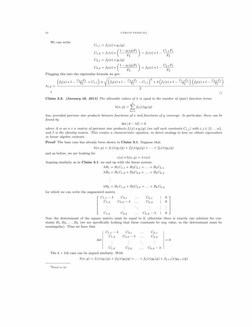
Plugging this into the eigenvalue formula we get:
λ1,2 =
(f2(x) ? 1− C2,1F1
F2+ C1,1
)±√(
f2(x) ? 1− C2,1F1
F2− C1,1
)2+ 4
(f1(x) ? 1− C1,1F1
F2
)(f2(x) ? 1− C2,1F1
F2
)2
3 �
Claim 3.3. (January 26, 2013) The allowable values of λ is equal to the number of (pair) function terms
h(x, y) =
n∑k=1
fk(x)gk(y)
has, provided pairwise star products between functions of x and functions of y converge. In particular, these can be
found bydet |A− λI| = 0
where A is an n× n matrix of pairwise star products fi(x) ? gj(y) (we call such constants Ci,j) with i, j ∈ {1 . . . n},and I is the identity matrix. This creates a characteristic equation, in direct analogy to how we obtain eigenvalues
in linear algebra contexts.
Proof The base case has already been shown in Claim 3.1. Suppose that
and as before, we are looking fore(x) ? h(x, y) = λ e(x)
Arguing similarly as in Claim 3.1, we end up with the linear system:
λB1 = B1C1,1 +B2C2,1 + . . .+BkCk,1
λB2 = B1C1,2 +B2C2,2 + . . .+BkCk,2
...
λBk = B1C1,k +B2C2,k + . . .+BkCk,k
for which we can write the augmented matrixC1,1 − λ C2,1 . . . Ck,1 | 0
C1,2 C2,2 − λ . . . Ck,2 | 0...
.... . .
......
...
C1,k C2,k . . . Ck,k − λ | 0
Now the determinant of the square matrix must be equal to 0, otherwise there is exactly one solution for con-stants B1, B2, . . . , Bk (we are specifically looking that these constants be any value, so the determinant must benonsingular). Thus we have that