Submitted tomanuscript XXXXXXXX

Compensating for Dynamic Supply Disruptions:Backup Flexibility Design

Soroush Saghafian1, Mark P. Van Oyen2

1 Industrial Eng., School of Computing, Informatics and Decision Systems Engineering Arizona State University, Tempe, AZ2 Dept. of Indust. & Oper. Eng., Univ. of Michigan, Ann Arbor, MI

To increase resilience in supply chains, we investigate the optimal design of flexibility in the backup system. Wemodel the dynamics of disruptions as Markov chains, and consider a multi-product, multi-supplier supply chain underdynamic disruption risks. Using our model, we first show that a little flexibility in the backup system can go a longway in mitigating dynamic disruption risks. This raises an important and fundamental question in designing flexibilityin the backup system: to achieve the benefits of full backup flexibility, which unreliable suppliers should be backed up?To answer this question, we connect the supply chain to various queueing and dam models by analyzing the dynamicsof the inventory shortfall process. Using this connection, we show that backing up suppliers merely based on firstmoment considerations such as their average reliability or average product demand can be misleading. All else equal,it is better to back up suppliers with (1) longer but less frequent disruptions, and (2) lower demand uncertainty. Inaddition to such second moment effects, by employing the Renyi’s Theorem, we demonstrate that when disruptionsare relatively long (if they occur), backing up the suppliers for which the expected wasted backup capacity is minimumprovides the best backup flexibility design. We also develop easy-to-compute and yet effective indices that (a) guidethe supply chain designer in deciding which suppliers to backup, and (b) provide insights into the role of variousfactors such as inventory holding and shortage costs, purchasing costs, suppliers reliabilities, and product demanddistributions in designing backup flexibility.

Key words : Backup Capacity; Flexibility; Dynamic Disruption Risk; Inventory Shortfall Process.History : Last Reversion: February 9, 2015.

1. Introduction

Some companies, like Ericsson, have learned the hard way that even minor incidents can cause

disruptions of major economic consequence. For Ericsson, a very small fire in a small production

cell was put out in ten minutes; however, the impact on a critical clean room resulted in a serious

loss of production capacity. Ultimately, $200M in insurance compensation was paid out (see, e.g.,

Norrman and Jansson 2004). While it is obvious that the frequency of supply disruptions varies

greatly depending on the products involved, the business practices in place, the transportation

modes, and stability of the political and infrastructural environment, disruptions are much more

frequent than is commonly recognized. A recent large-scale international survey performed by

Business Continuity Institute indicates that 85% of firms around the world experience at least

one supply chain disruption each year, and more than 50% face between one and five (Business

Continuity Institute, 2011). We are particularly motivated to study effective backup flexibility

designs for businesses with recurring disruptions.

Many firms, with electronics sector companies being among the leaders, are pursuing more rig-

1

Saghafian and Van Oyen: Dynamic Supply Disruptions: Backup Flexibility Design2 Article submitted to ; manuscript no. XXXXXXXX

orous business continuity and contingency plans. As identified in Norrman and Jansson (2004),

Ericsson now frames contracts with specific attention to the identification of and plans for response

at a backup site or resource. Ericsson is moving to incorporate both top tier suppliers and impor-

tant sub-suppliers into a risk management approach that considers both the length of disruptions

(recovery time) and their financial cost (Norrman and Jansson, 2004). Our study considers a micro-

economic model of the disruption cost in terms of backorders (and indirectly, inventory holding

costs when extra inventory is carried as a disruption mitigation strategy). We also introduce a

Markov chain model of disruptions that permits heterogeneity in the rate of supplier disruptions

(reliability) versus the mean length of the disruption duration (recovery time). This permits a busi-

ness analytics approach that can expose the importance of business recovery time in addition to

supplier reliability in pre-disruption planning. For example, we investigate in Section 4 the decision

of which of two suppliers is more important to back up when one has higher availability than the

other, but also longer disruption durations.

Investing in backup suppliers has been used by many leading companies. For example, Toyota

used it to reduce its exposure to disruptions (see Kim (2011)). Kouvelis and Li (2008) provide

an insightful description of a business environment that is particularly suited to this approach

of creating an emergency backup supplier for a single high disruption risk product, stating that

“Frequently, in just-in-time environments where the buyer (manufacturer) runs a continuous-flow

system for high-volume low-uncertainty goods (“functional goods” ...), the most frequent cause in

creating supply-demand mismatches is not demand uncertainty but unreliable supply...” While the

majority of studies focusing on the benefits of creating backup capacity develop models that are

essentially single-period, ours allows inventory to carry over, a mechanism that is typically used in

practice to mitigate disruptions.

As Tang (2006) posits, one of the fundamental strategies for increasing the robustness of the

supply chain is to increase the flexibility of the supply base. The area of operational flexibility

provides a rich landscape of paradigms which could be used to increase the flexibility of the supply

chain in the sense of better maintaining high service levels despite a disruption from a primary

supplier. In contrast to the traditional approach of providing an inflexible backup supplier, we note

that either full or partial flexibility in the backup supplier can be more economically attractive

than the traditional use of “dedicated” backups. Considering this, firms are increasingly thinking

about ways to create backup capacity in a flexible manner as an alternative to having a dedicated

backup supplier for every product or carrying extra inventories, which are both expensive practices.

It is often desirable (e.g., in the case of circuit board production or semiconductor manufacturing)

to have a single pooled flexible backup supplier that is capable of ensuring supply continuity (at

some capacity level) for multiple products in the event that one or more primary suppliers are

disrupted. This type of approach has received some attention to date (see, e.g., Tomlin and Tang

(2008) and Saghafian and Van Oyen (2012)).

Saghafian and Van Oyen: Dynamic Supply Disruptions: Backup Flexibility DesignArticle submitted to ; manuscript no. XXXXXXXX 3

It should be noted that process designs for a backup supplier’s operation may be quite differ-

ent than that for the primary supplier due to issues of volume and utilization. Particularly, when

the volumes are large, primary suppliers are likely to have assembly line processes, which provide

economy of scale at high volume but are usually expensive to make flexible. Unless the primary

supplier has very frequent disruptions, production is required only intermittently from the backup

supply infrastructure, and thus high volume assembly lines in the backup may not be economical.

Rather, it is more likely that such backup suppliers have job shop, batch, or reconfigurable produc-

tion processes, all of which are more flexible than automation-intensive assembly lines (and could

easily process a wide range of products in areas such as circuit board assembly or semiconductor

manufacturing). The higher the reliability of the primary supplier, the lower the average demand

for the backup supplier and the greater the barrier to justifying the investment in the backup

supplier. The above issues justify the “economy of scope” that can be harnessed by investing in

flexible backup manufacturing infrastructure.

While attractive, injecting full flexibility into the backup system is typically impossible due to

various technological and economical burdens. The choice to pool capacity in a backup supplier

when full flexibility is impossible, poses an interesting and fundamental pre-disruption risk man-

agement question: which suppliers should be backup by the flexible backup capacity? In fact, the

optimal design of backup flexibility is an important question in practice, which has not received

enough attention in the academic literature. It is our goal in this paper to fill this gap: we attempt

to generate insights into effective ways of designing flexibility in a supply chain backup system.

Importantly, we first show that a little flexibility in the backup system can go a long way in mit-

igating dynamic disruptions, suggesting that partial flexibility can effectively archive the benefits

of full flexibility for mitigating dynamic disruption risks. However, to achieve such benefits, the

partial flexibility should be designed intelligently. This, of course, is inextricably linked with the

ability to carry inventory over time and update inventory safeguards for different products as an

alternative way to mitigate disruptions.

To address the optimal design of flexibility in the backup system, we consider a supply chain

with limited backup capacity, multiple products, and multiple unreliable suppliers. We allow for

disruption risks to dynamically change over time, and model the dynamics of a supplier’s dis-

ruption risk as a Discrete Time Markov Chain (DTMC)1 with several threat levels indicating

the “health level” of suppliers. As one example, the S&P credit risk rating system with states

{1=AAA, 2=AA, 3=A, 4=BBB, 5=B/BB, 6=CCC/CC/C} ∪ {0 = Default} is an analogous

system for which Markov chain modeling is commonly used. We analyze the inventory shortfall

process (the difference between desirable inventory safeguards and inventory levels, a potentially

positive quantity due to a limited capacity when primary suppliers are disrupted) and connect it

to single-server queueing systems as well as dam storage processes.

1 Our Markov model is a step forward from the prevalent assumption of i.i.d. Bernoulli disruptions in the literaturewhich does not model the effect of the length of a disruption.

Saghafian and Van Oyen: Dynamic Supply Disruptions: Backup Flexibility Design4 Article submitted to ; manuscript no. XXXXXXXX

Using such a connection, we show that backing up suppliers merely based on first moment effects

such as their average reliability or product demand can be misleading. We find that, all else equal,

it is better to back up suppliers with (1) longer but less frequent disruptions, and (2) lower demand

uncertainty. These shed light on the important role of disruption lengths and demand variabilities

in design of backup flexibility. To generate further insights into the role of demand distributions

(not just the first and second moments), we also consider situations where disruptions are relatively

long when they occur, i.e., scenarios with long “time to recovery.” By using the Renyi’s Theorem

(which provides an approximation for geometric random sum of i.i.d. random variables) for the

inventory shortfall process under long disruptions, we show that, backing up the suppliers for

which the expected wasted backup capacity is minimum provides the best backup flexibility design.

Computing the expected wasted backup capacity requires the supply chain designer to evaluate

the cumulative distributions of the product demands at the available backup capacity. This sheds

further light on the role of demand distributions (not just their averages) on the design of backup

flexibility, especially in supply chains under long “time to recovery.”

After generating insights into the important effects of length of disruptions, demand variability,

and demand distributions, we factor out such effects, and focus on the role of other parameters

such as inventory holding and shortage costs and purchasing costs. We do this by (a) considering

the system under i.i.d. Bernoulli disruptions (a special case of our general Markov chain model)

and (b) assuming exponential demand distributions. Under these assumptions, the dynamics of

inventory shortfall process becomes equivalent to that of waiting time in a GI/M/1 queueing

system. Taking advantage of this equivalence, we characterize both the optimal inventory base-

stock levels and long-run average costs. In turn, this enables us to develop an easy-to-compute

and yet effective index, which we term Backup Effect Index (BEI), that (a) guides the supply

chain designer in deciding which suppliers to backup, and (b) provides interesting insights into the

role of various factors such as inventory holding and shortage costs, purchasing costs, suppliers

reliabilities, and product demands in designing backup flexibility. Our results suggest that, when

demand distributions are close to exponential, following a largest BEI policy is optimal in deciding

which unreliable suppliers to back up . We then extend this result by relaxing the exponential

demand assumptions (i.e., by considering general distributions) and analyzing a GI/GI/1 queueing

counterpart to the inventory shortfall process. This allows us to provide a generalized BEI (GBEI),

and show that in general backing up suppliers based on a largest GBEI first policy provides an

effective backup flexibility design, enabling supply chain designers to effectively compensate for

disruption risks.

To generate further insights into the role of capacity pooling in the backup system, we also

develop a numerical study and compare scenarios with dedicated backup suppliers versus a single

pooled backup capacity. We find that the value of a flexible backup supplier is more than the

summation of benefits that can be obtained separately for each of the products through dedicated

Saghafian and Van Oyen: Dynamic Supply Disruptions: Backup Flexibility DesignArticle submitted to ; manuscript no. XXXXXXXX 5

backups: when one of the primary suppliers is in a high threat level and the other is in a low

threat level, the pooled backup capacity can be shifted towards the unreliable supplier which is

at a higher risk. Moreover, we observe that a firm will reserve at least as much capacity from a

backup flexible supplier as the amount reserved in total from dedicated backup ones. Indeed, the

flexibility of a backup supplier provides the firm with greater benefits, justifying reserving more

backup capacity because of the economic advantage of shifting the orders whenever necessary. This

observation sheds light on higher fees charged in practice by flexible suppliers for reserving their

capacity compared to inflexible suppliers.

The remainder of the paper is organized as follows. We review the literature in the next section,

then in Section 3 we describe our model. Section 4 generates insights into the important role

of length of disruptions as well as demand variability in designing backup flexibility. Section 5

neutralizes the role of the factors studied in Section 4, and generates insights into the role of

some other important factors. Section 6 develops a numerical study and generates insights into the

capacity pooling advantage in the backup system. Section 7 summarizes the insights gained and

concludes. All proofs are presented in the Online Appendix.

2. Literature Review and Contributions

The operational literature on supply chain disruption risks can be viewed from two different per-

spectives: (A) time relative to the disruption event, and (B) the way the disruption event is

modeled.

From the perspective of time relative to the disruption event, Behdani et al. (2012) perform a

literature review and describe how the literature can be classified in three categories: (A.1) pre-

disruption studies, (A.2) post-disruption studies, and (A.3) integrated studies of both pre- and

post-disruptions. Most disruption management studies fall into the first two categories. This paper

is among the very few studies to consider both pre- and post-disruptions. We treat several common

pre-disruption approaches to supply flow continuity: carrying additional inventory, investing in

backup capacity, and taking into consideration the dynamics of a supplier’s likelihood of disruption

(i.e., dynamic supplier monitoring and assessment of its threat level). As a post-disruption mech-

anism, the modeling of dynamic inventory replenishment policies is especially meaningful in this

paper. We consider not only inflexible backup suppliers (which also require a capacity investment

decision), but also the proper dynamic use of a pooled flexible backup supplier that can serve

multiple products out of its shared but limited capacity (in response to disruptions in unreliable

suppliers).

Whether static (e.g., single-shot or repeated settings) or dynamic, the literature models disrup-

tions in the following four categories: (B.1) random disruptions (i.e., all-or-nothing), (B.2) random

yield, (B.3) random capacity, and (B.4) financial default. This paper is in the first category, dynamic

random disruptions.

For studies that consider the case of random disruptions, we refer interested readers to Parlar

Saghafian and Van Oyen: Dynamic Supply Disruptions: Backup Flexibility Design6 Article submitted to ; manuscript no. XXXXXXXX

and Perry (1996), Gurler and Parlar (1997), Moinzadeh and Aggarwal (1997), Arreola-Risa and

DeCroix (1998) Tomlin (2006), Babich et al. (2007), Saghafian and Van Oyen (2012), and the

references therein. Some studies including Wang et al. (2010) consider a combination of the above-

mentioned types of disruptions. Moreover, while most studies have focused on static disruptions, a

few consider dynamic of disruptions. Tomlin and Snyder (2006), for instance, develop multi-period

models with dynamic disruptions in which the firm has a single unreliable supplier, as well as

models with a second, perfectly reliable supplier. Tomlin (2006) considers dynamic disruption risks

in a single-product setting with two dedicated suppliers: one perfectly reliable and one unreliable.

When the amount ordered from the reliable supplier is a fixed percentage of the demand in each

period, Tomlin (2006) establishes the optimality of a state-dependent base-stock policy. Dong and

Tomlin (2012) consider a setting that operationally resembles the disruption model of Tomlin

(2006) to study the interplay between business interruption insurance and operational measures.

The inventory control literature with Markovian supply availability is also to some extent relevant

to our study, although it typically studies single-sourcing models without any supply flexibility.

Within this literature, Song and Zipkin (1996) present a fundamental study with periodic review

inventory control where information about the evolution of the supply system is modeled as a

Markov chain. Parlar et al. (1995) addresses a periodic-review setting with setup costs, where the

probability that an order placed now is filled in full depends on whether supply was available in

the previous period (see also Ozekici and Parlar (1999)). We contribute a new perspective by using

the connections between the dynamics of inventory shortfall process (under dynamic disruptions)

and various queueing and dam storage processes.

Another part of the literature includes multi-period models with repeated (but not dynamic)

disruptions. Tomlin (2009) uses a Bayesian approach for supply learning (i.e., reliability-forecast

updating) with i.i.d. Bernoulli disruptions and characterizes the firm’s optimal sourcing and inven-

tory decisions. Anupindi and Akella (1993) study a finite-horizon, discrete-time continuous demand

model with two zero lead-time random-yield suppliers.

In addition to considering a multi-period dynamic disruption model with an arbitrary number

of suppliers, another distinct feature of our modeling framework is that we allow for product mix

flexibility in the backup system, and study how such flexibility can be used to selectively supplement

the production of primary suppliers based on the firm’s inventory levels and suppliers’ threat levels.

Operational mix flexibility has been studied in various papers including Jordan and Graves (1995),

Van Mieghem (1998), Kouvelis and Vairaktarakis (1998), Graves and Tomlin (2003), Tomlin and

Wang (2005), Iravani et al. (2005), Bassamboo et. al. (2010), Saghafian and Van Oyen (2011,

2012), Simchi-Levi and Wei (2012), and Simchi-Levi et al (2013). Our study contributes to this

literature by (1) considering the value of a flexible pooled backup supplier/resource to compensate

for unreliability of dedicated suppliers, and (2) addressing the design of partial flexibility in the

backup system.

Saghafian and Van Oyen: Dynamic Supply Disruptions: Backup Flexibility DesignArticle submitted to ; manuscript no. XXXXXXXX 7

3. The Model

The model is a multi-period and multi-product extension of the one in Saghafian and Van Oyen

(2012) under a generalized capacity investment and flexibility setting. For readability, we employ

the same notation where possible. Consider a firm that produces/sells n = |N | products, where

N = {1,2, · · · , n} denotes the set of underlying products. The firm has a primary unreliable sup-

plier, labeled supplier j, that supplies product j ∈N (or perhaps one critical component for that

product). To operationally insure the supply stream against future disruptions, the firm can also

establish (or contract with) a flexible backup resource, namely f , at a limited capacity Qf ∈ (0,∞)

that can produce on demand quantities of underlying products, the sum of which cannot exceed Qf .

We let g(uf , Qf ) denote the investment cost at the flexible backup capacity, which depends on the

capacity level Qf as well as a “per unit” investment cost, uf . We allow for a general class of invest-

ment costs represented through the cost function g(uf , Qf ). However, to represent a “well-behaved”

investment cost function, we assume g : R2+→ R+ is continuous, increasing in uf with g(0, ·) = 0,

increasing convex in capacity Qf with g(·,0) = 0, and supermodular (twice differentiable with pos-

itive cross partials). We note that a special case of this type of investment is that of reserving some

backup capacity through a capacity reservation contract (also known as an option contract), where

an up-front cost of g(uf , Qf ) = ufQf reserves a backup capacity of Qf units (see, e.g., Saghafian

and Van Oyen (2012) and the references therein). We also permit a product-dependent per unit

ordering cost cfj from the backup. For convenience, we use subscripts for products, superscripts for

suppliers, and employ the following notation (j ∈N ):

hj : Holding cost per unit of product j per period;

pj : Penalty cost per unit of unmet demand of product j;

rj : Revenue per unit of product j (equal to zero when unmet demand is backlogged);

cj : Per unit purchasing cost of product j from dedicated/primary supplier j;

cfj : Per unit purchasing cost of product j from the flexible backup supplier;

uf : Per unit capacity reservation cost of the flexible backup supplier;

Qf : Reserved capacity from flexible backup supplier;

g(uf , Qf ) : Investment cost function at the flexible backup capacity;

qj : Order quantity from dedicated/primary supplier j;

qfj : Order quantity from flexible backup supplier for product j.

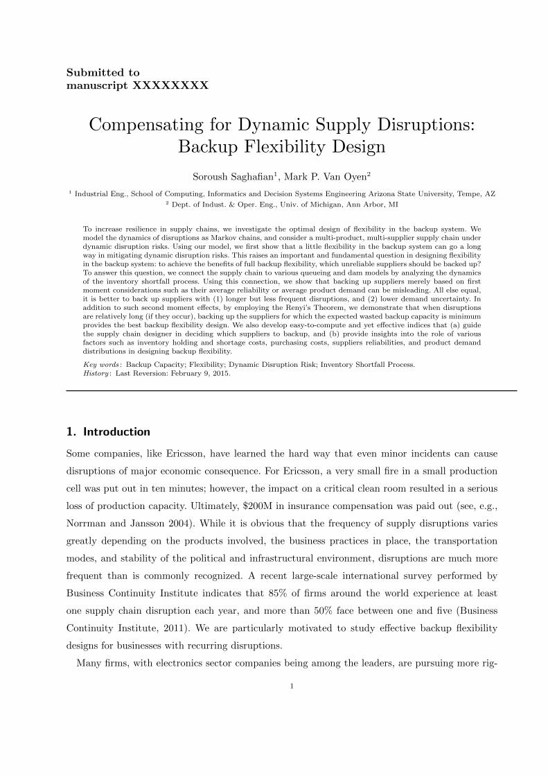
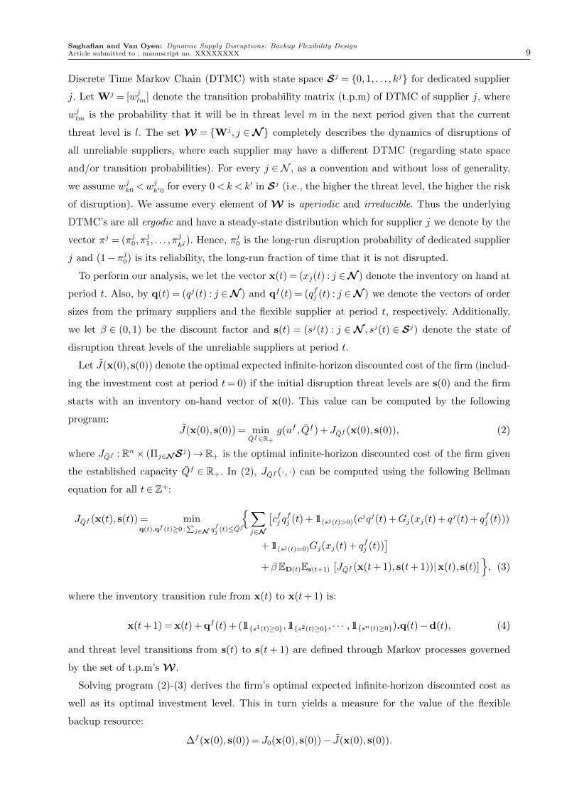
Fig. 1 depicts the two-echelon supply chain model under consideration2. The firm has an option

to establish (or reserve) a desired amount of flexible backup capacity, Qf , at time 0 to insure

its supply system against future disruptions. The firm then exercises a periodic review inventory

control in every future period, during which it can procure either from the primary suppliers or

2 We note that Fig. 1 (which is our focus) may only depict part of a supply chain: we only treat the n productsthat have particularly unreliable suppliers and so the flexible backup need only cover these n suppliers modeled. Thismodel also treats the extension to subsets of products forming a partition, each with a fully flexible backup suppliersfor one subset of products in the partition. As we will see, our model also allows for partial flexibility.

Saghafian and Van Oyen: Dynamic Supply Disruptions: Backup Flexibility Design8 Article submitted to ; manuscript no. XXXXXXXX

Primary 1

f

The Firm

1 Product

1q Markov Stochastic Disruptions

Markov Stochastic Disruptions

1F

nF nn hp ,

11,hp

n Product Stochastic Demand for Product n

Primary n

n Unreliable Suppliers

Flexible Backup Capacity fQ

nq

.

.

.

.

.

.

fq1

fn

j

fj Qq ≤∑

=1

nW

Primary 2

2 Product

. . .

Stochastic Demand for Product 1

Stochastic Demand for Product 2

2F

nW Markov

Stochastic Disruptions

2W

fq2

2q

fnq

Figure 1 The model with n products, n primary suppliers, and one flexible backup supplier. The up front invest-ment in backup capacity Qf and dynamic resupply orders are based on inventory levels and availableinformation on supplier threat levels, which evolve as Markov chains.

from the limited reserved backup flexible capacity or both. Unmet demand is backordered and

supply lead times and production cycles are negligible in comparison with the review period. We

assume the following order of events within each review period: (1) The firm observes the state of

the system (inventory levels and disruption threat levels). (2) The firm decides the order sizes and

orders from all suppliers subject to the contracts. (3) Product demands are realized. (4) Holding

costs or shortage costs accrue. (5) The state of the system is updated, including the inventory and

disruption threat levels. The firm has to pay the purchasing cost cj and cfj per order of product j ∈

N delivered by dedicated (and unreliable) supplier j and the flexible backup resource, respectively.

The flexible backup resource has a shared and limited capacity Qf (a decision variable). It can

deliver any combination and quantity of products (qfj : j ∈N ) as long as∑

j∈N qfj ≤ Qf . We assume

none of the products in set N can be procured for free; cfj +uf > 0 and cj > 0 for j ∈N .

To address the optimal design of flexibility in the backup system, we may also allow for only

a subset of the product types to share the flexible backup. This is done by defining a flexibility

set F , {j ∈N : cfj <∞}, and requiring it to be a strict subset of N . When F = N , we say the

backup supplier is fully flexible, and when F ⊂N , we say the backup supplier is partially flexible.

For j ∈N , let Lj(x) = hj[x]+ + pj[−x]+ and define the expected one-stage cost

Gj(x) =EDj [Lj(x−Dj)] = hj

∫ x

−∞(x− ξ)dFj(ξ) + pj

∫ ∞x

(ξ−x)dFj(ξ), (1)

where [x]+ = max {0, x}, and Fj(·) is the cumulative distribution function (c.d.f) of the demand,

Dj, for product j. We assume that demands for each product j across periods are i.i.d. random

variables, and further, Dj and Dj′ are independent (for all j, j′ ∈N s.t. j 6= j′). We also assume

unmet demand in a period is backlogged.

We model the disruption risk processes of the dedicated suppliers via a discrete time Markov

process. Let sj denote the threat level of dedicated supplier j (as an indicator of its health),

where sj = 0 means dedicated supplier j is in the down (default) state and sj = k > 0 denotes

that it is in threat level k. We assume that the dynamics of disruptions can be modeled as a

Saghafian and Van Oyen: Dynamic Supply Disruptions: Backup Flexibility DesignArticle submitted to ; manuscript no. XXXXXXXX 9

Discrete Time Markov Chain (DTMC) with state space Sj = {0,1, . . . , kj} for dedicated supplier

j. Let Wj = [wjlm] denote the transition probability matrix (t.p.m) of DTMC of supplier j, where

wjlm is the probability that it will be in threat level m in the next period given that the current

threat level is l. The set W = {Wj, j ∈N } completely describes the dynamics of disruptions of

all unreliable suppliers, where each supplier may have a different DTMC (regarding state space

and/or transition probabilities). For every j ∈ N , as a convention and without loss of generality,

we assume wjk0 <wjk′0 for every 0<k < k′ in Sj (i.e., the higher the threat level, the higher the risk

of disruption). We assume every element of W is aperiodic and irreducible. Thus the underlying

DTMC’s are all ergodic and have a steady-state distribution which for supplier j we denote by the

vector πj = (πj0, πj1, . . . , π

j

kj). Hence, πj0 is the long-run disruption probability of dedicated supplier

j and (1−πj0) is its reliability, the long-run fraction of time that it is not disrupted.

To perform our analysis, we let the vector x(t) = (xj(t) : j ∈N ) denote the inventory on hand at

period t. Also, by q(t) = (qj(t) : j ∈N ) and qf (t) = (qfj (t) : j ∈N ) we denote the vectors of order

sizes from the primary suppliers and the flexible supplier at period t, respectively. Additionally,

we let β ∈ (0,1) be the discount factor and s(t) = (sj(t) : j ∈N , sj(t) ∈ Sj) denote the state of

disruption threat levels of the unreliable suppliers at period t.

Let J(x(0), s(0)) denote the optimal expected infinite-horizon discounted cost of the firm (includ-

ing the investment cost at period t= 0) if the initial disruption threat levels are s(0) and the firm

starts with an inventory on-hand vector of x(0). This value can be computed by the following

program:J(x(0), s(0)) = min

Qf∈R+

g(uf , Qf ) +JQf (x(0), s(0)), (2)

where JQf : Rn× (Πj∈NSj)→R+ is the optimal infinite-horizon discounted cost of the firm given

the established capacity Qf ∈ R+. In (2), JQf (·, ·) can be computed using the following Bellman

equation for all t∈Z+:

JQf (x(t), s(t)) = minq(t),qf (t)≥0 :

∑j∈N q

fj (t)≤Qf

{∑j∈N

[cfj q

fj (t) + 11(sj(t)>0)(c

jqj(t) +Gj(xj(t) + qj(t) + qfj (t)))

+ 11(sj(t)=0)Gj(xj(t) + qfj (t))]

+βED(t)Es(t+1) [JQf (x(t+ 1), s(t+ 1))|x(t), s(t)]}, (3)

where the inventory transition rule from x(t) to x(t+ 1) is:

x(t+ 1) = x(t) + qf (t) + (11{s1(t)≥0},11{s2(t)≥0}, · · · ,11{sn(t)≥0}).q(t)−d(t), (4)

and threat level transitions from s(t) to s(t+ 1) are defined through Markov processes governed

by the set of t.p.m’s W .

Solving program (2)-(3) derives the firm’s optimal expected infinite-horizon discounted cost as

well as its optimal investment level. This in turn yields a measure for the value of the flexible

backup resource:

∆f (x(0), s(0)) = J0(x(0), s(0))− J(x(0), s(0)).

Saghafian and Van Oyen: Dynamic Supply Disruptions: Backup Flexibility Design10 Article submitted to ; manuscript no. XXXXXXXX

For instance, ∆f (x(0) = 01×n, s(0) = 11×n) provides a good measure for investigating the value of

the flexible backup resource by setting all initial inventory levels to zero and placing all suppliers

in their most reliable state.

In addition to the discounted cost, we may also use the firm’s long-run average inventory related

per-period cost average inventory related costs (holding and backlogging only), since it is a more

convenient measure for the purpose of connecting the inventory related cost of the system to the

queueing or dam storage processes. The long-run average inventory related per-period cost under

any given backup capacity Qf can be obtained from (3), and is defined as:

lim infβ→1−

(1−β)JQf (x, s).

4. Backup Flexibility Design: The Role of Disruption Length and DemandVariability

In this section, we analyze the optimal design of flexibility in the backup system, and generate

insights into the important role of disruption length and demand variabilities. To this end, we

consider the case of partial backup flexibility in which the backup flexibility can cover only a subset

of products N that belong to the flexibility set F , {j ∈N : cfj <∞}.

Before considering systems with partial flexibility, however, we shall establish a basic result under

full flexibility: firms that procure relatively more products benefit more from establishing a fully

flexible backup supplier, but the marginal benefit diminishes.

Proposition 1 (Diminishing Rate of Return). Under full flexibility (F = N ) and complete

product symmetry (product or supplier independent parameters), the value of a fully flexible backup

supplier has a diminishing rate of return (increasing concave) in |N |.

Comparing systems with full backup flexibility (F = N ) and with partial backup flexibility

(F ⊂N ) under full product symmetry, we next establish an important insight: for mitigating

dynamic disruption risks, a little backup flexibility can go a long way.

Proposition 2 (Partial Backup Flexibility). Consider a system with full product symmetry,

and fix the product set N . The difference between the value of the flexible backup supplier with

flexibility set N (full backup flexibility) and with F ⊂N (partial backup flexibility) is decreasing

and convex in the number of products in F .

The above proposition suggests that, under product symmetry, partial backup flexibility provides

a diminishing rate of return, and may rapidly achieve the benefit of full flexibility as F grows

to include more product types. Under asymmetry, intuition suggests that backing up some of the

suppliers will suffice in many cases. It is also important to consider that in practice there may be

a constraint that limits or eliminates how much flexibility the backup supplier may have. These

motivate the following question.

Question 1. Under asymmetry, which unreliable supplier(s) should be backed up first?

Saghafian and Van Oyen: Dynamic Supply Disruptions: Backup Flexibility DesignArticle submitted to ; manuscript no. XXXXXXXX 11

Intuition suggests that one should prioritize backing up the most unreliable supplier (lowest per-

centage uptime) or the supplier of the most “popular” product (highest average product demand).

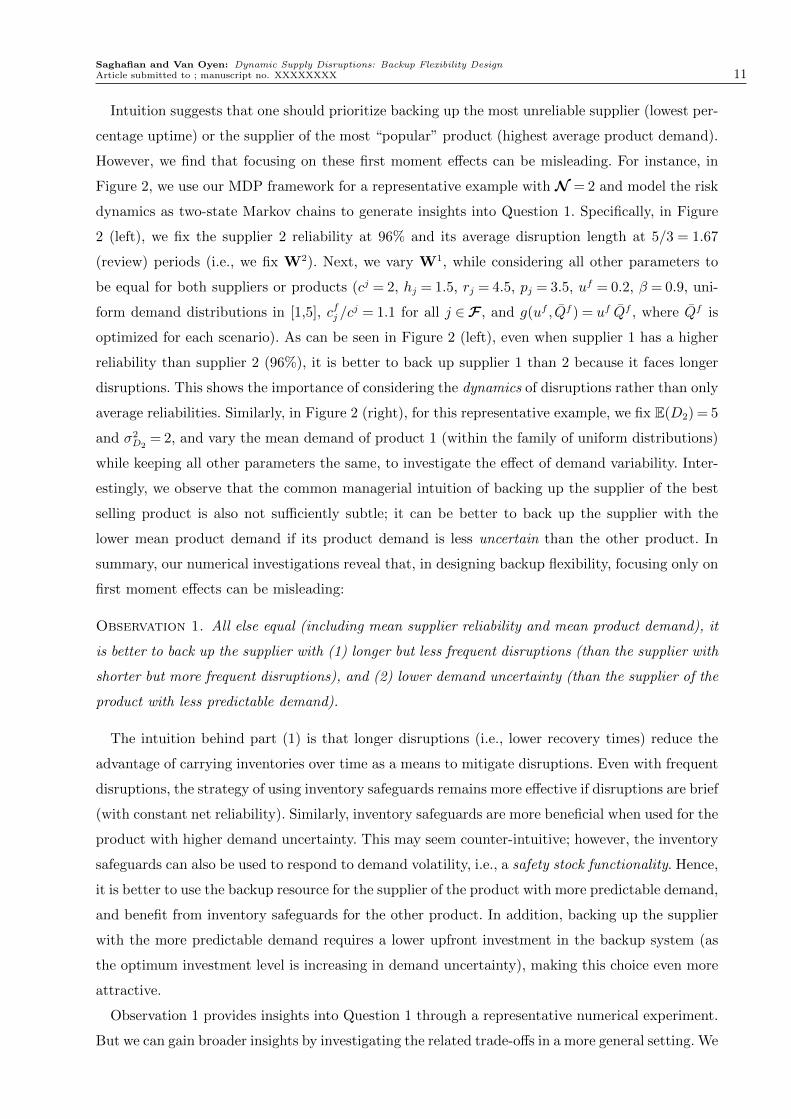
However, we find that focusing on these first moment effects can be misleading. For instance, in

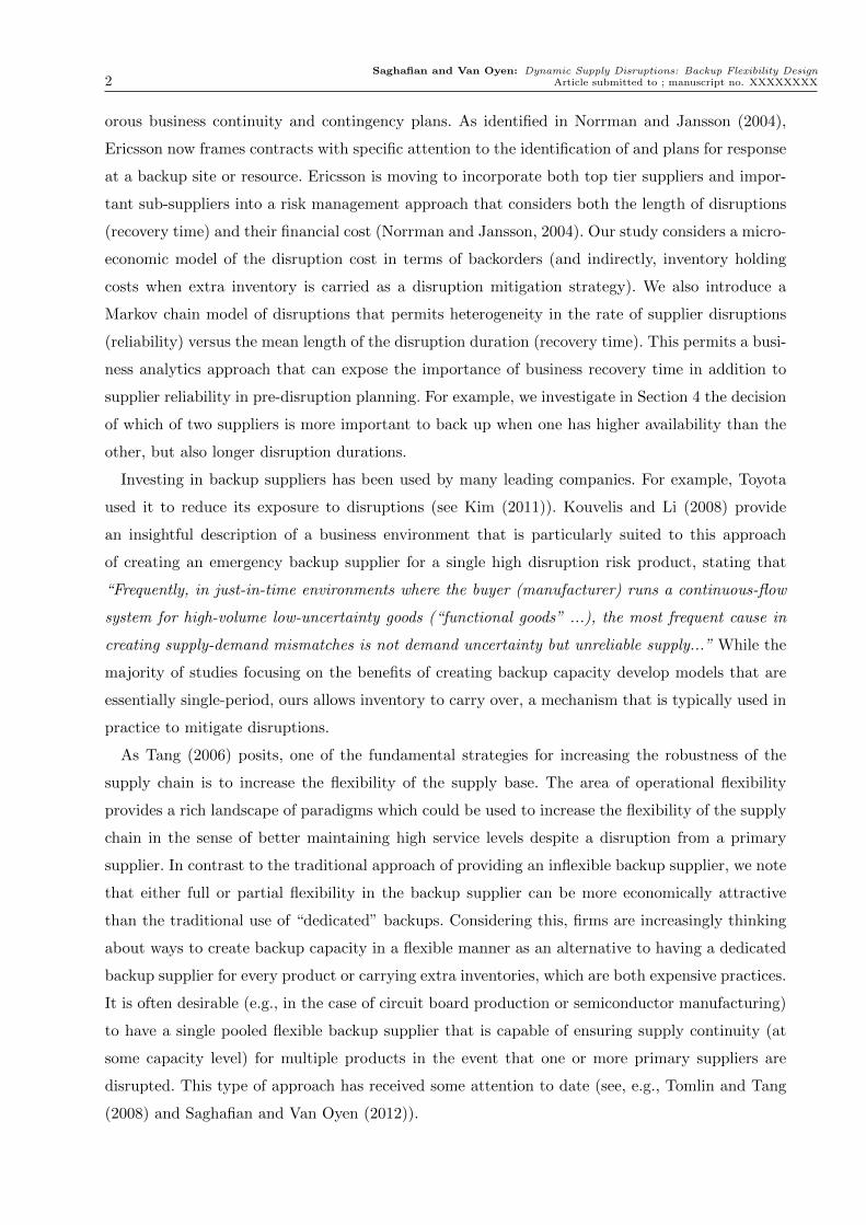
Figure 2, we use our MDP framework for a representative example with N = 2 and model the risk

dynamics as two-state Markov chains to generate insights into Question 1. Specifically, in Figure

2 (left), we fix the supplier 2 reliability at 96% and its average disruption length at 5/3 = 1.67

(review) periods (i.e., we fix W2). Next, we vary W1, while considering all other parameters to

be equal for both suppliers or products (cj = 2, hj = 1.5, rj = 4.5, pj = 3.5, uf = 0.2, β = 0.9, uni-

form demand distributions in [1,5], cfj /cj = 1.1 for all j ∈F , and g(uf , Qf ) = uf Qf , where Qf is

optimized for each scenario). As can be seen in Figure 2 (left), even when supplier 1 has a higher

reliability than supplier 2 (96%), it is better to back up supplier 1 than 2 because it faces longer

disruptions. This shows the importance of considering the dynamics of disruptions rather than only

average reliabilities. Similarly, in Figure 2 (right), for this representative example, we fix E(D2) = 5

and σ2D2

= 2, and vary the mean demand of product 1 (within the family of uniform distributions)

while keeping all other parameters the same, to investigate the effect of demand variability. Inter-

estingly, we observe that the common managerial intuition of backing up the supplier of the best

selling product is also not sufficiently subtle; it can be better to back up the supplier with the

lower mean product demand if its product demand is less uncertain than the other product. In

summary, our numerical investigations reveal that, in designing backup flexibility, focusing only on

first moment effects can be misleading:

Observation 1. All else equal (including mean supplier reliability and mean product demand), it

is better to back up the supplier with (1) longer but less frequent disruptions (than the supplier with

shorter but more frequent disruptions), and (2) lower demand uncertainty (than the supplier of the

product with less predictable demand).

The intuition behind part (1) is that longer disruptions (i.e., lower recovery times) reduce the

advantage of carrying inventories over time as a means to mitigate disruptions. Even with frequent

disruptions, the strategy of using inventory safeguards remains more effective if disruptions are brief

(with constant net reliability). Similarly, inventory safeguards are more beneficial when used for the

product with higher demand uncertainty. This may seem counter-intuitive; however, the inventory

safeguards can also be used to respond to demand volatility, i.e., a safety stock functionality. Hence,

it is better to use the backup resource for the supplier of the product with more predictable demand,

and benefit from inventory safeguards for the other product. In addition, backing up the supplier

with the more predictable demand requires a lower upfront investment in the backup system (as

the optimum investment level is increasing in demand uncertainty), making this choice even more

attractive.

Observation 1 provides insights into Question 1 through a representative numerical experiment.

But we can gain broader insights by investigating the related trade-offs in a more general setting. We

Saghafian and Van Oyen: Dynamic Supply Disruptions: Backup Flexibility Design12 Article submitted to ; manuscript no. XXXXXXXX

Supplier 1

Supplier 2

92 93 94 95 96 97 981

2

3

4

5

6

7

Supplier 1 Reliability H%L

Supp

lier

1D

isru

ptio

nL

engt

hHP

erio

dsL

Supplier 2

Supplier 1

4.0 4.5 5.0 5.5 6.0 6.5 7.00

1

2

3

4

Supplier 1 Avg. Demand

Supp

lier

1D

eman

dV

aria

nce

Figure 2 Which supplier to back up? Left: Effect of disruption length (supplier 2 reliability =96%, supplier 2avg. disruption length = 5/3); Right: Effect of demand uncertainty (E(D2) = 5, σ2

D2= 2).

do this by introducing and exploring the dynamics of threat-dependent inventory shortfall3, which

is the difference between the threat-dependent base-stock levels and the inventory level caused

by the limited supply capacity during disruptions as well as the random demand realizations. In

particular, we will observe that the dynamics of threat-dependent inventory shortfalls resemble

the waiting time of a customer in a single-server G/GI/1 type queue where the distribution of

inter-arrival times is given by a two-state deterministic Markov modulated process. This fact along

with an analogous simple dam/storage process enables us to answer Question 1 in more depth.

To this end, consider two suppliers indexed by j = 1,2 that have the same average reliability,

but let supplier 1 experience longer (in terms of first order stochastic dominance) but less frequent

disruptions than supplier 2. For simplicity, we assume both suppliers have the same threat level

state space denoted by S ,S1 =S2. If the transition probability matrices Wj = [wjlm]l,m∈S are such

that w100 ≥w2

00 but π10 = π2

0, then the required conditions hold. In particular, while both suppliers

have the same average reliability (1−πj0), the geometric random variables representing the length

of disruptions denoted by Lj satisfy L2 ≤st L1, where ≤st denotes first order stochastic dominance.

Moreover, since π10 = π2

0, we have that the frequency of disruptions∑

i∈S,i6=0 πji w

ji0 is higher for

supplier 2 than supplier 1. Using this setting, we first study the effect of disruption length in the

absence of any backup capacity, and then extend the result to situations where they can be backed

up. To do so, we note that the firm’s product j inventory at the beginning of period t+ 1 under

the optimal base-stock inventory control policy is recursively given by

Xjt+1 = min{Xj

t −Djt +Kj(sjt), y

j(sjt)}, (5)

where yj(sjt) is the base-stock level of product j when its supplier’s threat level at period t is sjt , Djt

denotes the demand of product j at period t, and Kj(sjt) can be thought of as a state-dependent

“random supply capacity” (of supplier j when its threat level at period t is sjt): Kj(sjt) = 11{sjt 6=0}M ,

3 For analysis of regular inventory shortfall in traditional inventory models with a single, fully reliable supplier (underlimited capacity) we refer to Tayur (1993) and Glasserman (1997).

Saghafian and Van Oyen: Dynamic Supply Disruptions: Backup Flexibility DesignArticle submitted to ; manuscript no. XXXXXXXX 13

for some sufficiently large number M that approximates the capacity of the backup supplier.4

Denote by Ψjt(s

jt) = yj(sjt)−Xj

t the threat-dependent inventory shortfall of product j at period t.

Then, Ψjt(s

jt) can be recursively written as:

Ψjt+1(sjt+1) = max{Ψj

t(sjt)−Kj(sjt) +Dj

t ,0}. (6)

The dynamics of threat-dependent inventory shortfall presented above is similar to that of the

waiting time (in queue) of the t-th customer in a single server queueing system with inter-arrival

and service times being represented by Kj(sjt) and Djt , respectively. However, first it should be

noted that this interpretation of the shortfall as a waiting time is not intuitive and differs from

manufacturing queues where time is continuous and queues are discrete: the shortfall in period t

in our framework is interpreted as the waiting time (in queue) of customer t, and hence, time is

discrete while queues are continuous. Second, we note that if the “random supply capacity” was

not threat-dependent (i.e., random variables Kj(sjt) were i.i.d. across periods), then the Lindley

type dynamics presented in (6) would be exactly the same as that of waiting time (in queue) of

a customer in a GI/GI/1 queueing system. However, (6) shows that the dynamics of shortfall is

threat-dependent and resemble the waiting time (in queue) of a customer in a G/GI/1 queueing

system in which the inter-arrival times (random variable Kj(sjt)) are deterministically defined based

on an exogenous two-state Markov-modulated process: Kj(sjt) = 11{sjt 6=0}M .

Since the Markov chain describing the dynamics of sjt is ergodic, both sjt and sjt+1 converge

in distribution (denoted byd→) to the same random variable sj as t→∞, which has the distri-

bution πj (i.e., the steady-state distribution). Hence, there exists a random variable Kj(sj) such

that Kjt (s

jt)

d→Kj(sj) as t→∞. Thus, assuming that the underlying queueing system is stable,

Ψjt+1(sjt+1)

d→Ψj(sj) where

Ψj(sj)d= max{Ψj(sj)−Kj(sj) +Dj,0}. (7)

Using the discussion above, we first note that the firm’s long-run average inventory cost associated

with product j (under a threat-dependent base-stock yj(sj)) is:

Esj ,Ψj(sj),Dj[hj(y

j(sj)−Ψj(sj)−Dj)++ pj(Dj + Ψj(sj)− yj)+

]= Esj ,Ψj(sj)

[Gj(y

j(sj)−Ψj(sj))]

=∑

i∈S,S1=S2

πji EΨj(i)

[Gj(y

j(i)−Ψj(i))],(8)

where Gj(·) is defined in (1). Moreover, to use (8), it can be easily seen that:

EΨj(i)

[Gj(y

j(i)−Ψj(i))]

= hj

∫ yj(i)

−∞(yj(i)− ξ)dFDj+Ψj(i)(ξ)+pj

∫ ∞yj(i)

(ξ−yj(i))dFDj+Ψj(i)(ξ), (9)

where FDj+Ψj(i) is the convolution of distributions of demand, Dj, and shortfall, Ψj(i) (by inde-

pendence). Since the above function is convex (due to convexity of Gj(·)), it follows from the first

order condition that the optimal base-stock level satisfies:

4 We consider M to be a sufficiently large number throughout this paper, but our results rigorously follow by takingthe limit as M goes to infinity

Saghafian and Van Oyen: Dynamic Supply Disruptions: Backup Flexibility Design14 Article submitted to ; manuscript no. XXXXXXXX

Pr(Dj ≤ yj(i)−Ψj(i)

)=EΨj(i)

[F jD(yj(i)−Ψj(i))

]=

pjpj +hj

, (10)

or equivalently

yj(i) = F−1Dj+Ψj(i)

(pj

pj +hj), (11)

where for any random variable Ξ with a c.d.f. FΞ(ξ),

F−1Ξ (y) = inf

{ξ : FΞ(ξ)≥ y

}. (12)

Replacing the optimal base-stock level characterized by (11) in (8) and (9) will enable us to

compare the optimal cost of product/supplier 1 to that of product/supplier 2. Using this, we first

establish that a stochastically larger “waiting time” (in queue) in the corresponding queueing

system means both a higher optimal base-stock level and cost in the original inventory system.

This will later enable us to show the important insight that, keeping average reliability the same,

longer but less frequent disruptions cause higher average costs.

Lemma 1 (Queueing Comparison). In the absence of any backup capacity, if Ψ2(i) ≤st Ψ1(i)

(for all i∈S ,S1 =S2 ), then (i) the state-dependent optimal base-stock levels satisfy y2(i)≤ y1(i),

and (ii) having only product 2 is preferred to having only product 1: N = {1} �N = {2}, where �

represents preference in terms of associated expected long-run average cost.

We next show that longer but less frequent disruptions (all else equal including average reliabil-

ities) indeed implies a stochastically larger “waiting time” in the corresponding queueing system

(i.e., larger shortfalls in the inventory system), which is analogous to a well-known fact in queue-

ing systems: a stochastically higher inter-arrival time variability typically implies a longer average

waiting time. To show this result, we consider the following dam model or storage process5 with

an input Dt at the beginning of period t. In each period, a decision regarding whether to open the

dam is made: the dam is kept completely closed if st = 0, and is completely opened (i.e., instanta-

neous release) otherwise. This dam model allows us to characterize the threat-dependent inventory

shortfall as a compound random variable (i.e., a random sum of i.i.d. random variables) and state

the following.

Lemma 2 (Role of Disruption Length). In the absence of any backup capacity, the inventory

shortfall of product j given risk state i (for all i∈S ,S1 =S2) satisfies

Ψj(i)d= 11{i=0}

Lj∑t=1

Dt, (13)

where random variables Dt are i.i.d., and Dt is the demand in period t. Hence, if supplier 1 has

longer but less frequent disruptions than supplier 2 but all else is equal, then in the absence of any

backup capacity Ψ2(i)≤st Ψ1(i) (for all i∈S ,S1 =S2).

5 See, e.g., Prabhu (1965) and Tayur (1993) for some results on inventory models with single, fully reliable, butcapacitated suppliers.

Saghafian and Van Oyen: Dynamic Supply Disruptions: Backup Flexibility DesignArticle submitted to ; manuscript no. XXXXXXXX 15

It is noteworthy that while the base-stock levels are different for different threat-levels, the

shortfall process characterized in the above lemma only depends on whether the system is up or

down, providing a much simpler process to analyze.

Combining Lemmas 1 and 2 we observe that, in the absence of any backup capacity, if supplier 1

has longer but less frequent disruptions than supplier 2, then (a) the firm tends to keep stochasti-

cally higher levels of on-hand inventory of product 1 than 2, and (b) product 1 is associated with

a higher optimal average cost. The following lemma extends this result to the case where a given

secondary capacity can be assigned to back up unreliable suppliers.

Lemma 3 (Disruption Length and Backup Capacity). When a given capacity Qf is assigned

to back up supplier j ∈ {1,2}, for all i∈S ,S1 =S2

Ψj(i)d= 11{i=0}

Lj∑t=1

(Dt− Qf )+. (14)

Hence, if supplier 1 has longer but less frequent disruptions than supplier 2 but all else is equal,

then (i) Ψ2(i)≤st Ψ1(i) (for all i∈S ,S1 =S2), and (ii) N = {1} �N = {2}.

In addition to characterizing the effect of backup capacity on inventory shortfall, the above

lemma shows that disruption length and backup capacity are substitutes: the effect of a longer

disruption length can be offset by a higher backup capacity level. Using the above lemma, we

next establish the interesting insight that when a backup capacity exists, it is better to back up

the supplier with longer but less frequent disruptions (all else equal). Recalling the problem of

determining the optimal flexibility set F (which indicates the set of suppliers to backup), this

insight is presented in the following result.

Proposition 3 (The Effect of Disruption Length on Backup Flexibility Design). Let

N = {1,2}, and while keeping all else equal (including average reliabilities), suppose supplier 1

has longer but less frequent disruptions than supplier 2. (i) For any available backup capacity Qf ,

F = {2} �F = {1} �F = {1,2}. (ii) Part (i) holds even when the backup capacity is optimized

separately for each of the three flexibility designs.

We note that the above result establishes an important insight in designing backup flexibility: the

length of disruptions plays a critical role in deciding which supplier(s) to back up. Therefore, paying

attention only to suppliers’ average relabilities can be misleading: it might be better to backup

a supplier with higher average reliability, if its disruptions are lengthier. Moreover, Proposition 3

can be easily extended to a setting with an arbitrary number of products as follows. Let N =

{1,2, . . . , n} for some n, and suppose that suppliers are only different in their length of disruption in

the sense of stochastic dominance while all else is equal. If only a partial flexibility with |F |= k < n

is possible, then the optimal backup flexibility design is the one in which F is chosen to be the set

of k suppliers with the lengthiest disruptions: a longest disruption length first policy. This agrees

with the focus on “time to recover” recently emphasized in Simchi-Levi et al. (2014).

Saghafian and Van Oyen: Dynamic Supply Disruptions: Backup Flexibility Design16 Article submitted to ; manuscript no. XXXXXXXX

We now turn our attention from the supply side to the demand side. Specifically, we establish

that, similar to the supply side, merely paying attention to the average demand can be misleading.

To this end, we can again benefit from the dynamics of inventory shortfall. Since a higher

demand variability in the original system implies a higher service time variance in the queueing

counterpart, and the performance of queueing systems typically is roughly inversely proportional

to service time variance, we can explore the answer to Question 1 in more depth. This is done in

the following proposition, where variability is captured through convex stochastic ordering.

Proposition 4 (The Effect of Demand Variability on Backup Flexibility Design).

Let N = {1,2}, and while keeping all else equal (including average demand for products 1 and

2), suppose D1 ≤cx D2 (where ≤cx denotes convex stochastic ordering6), implying that demand

for product 2 has a higher variability than product 1. (i) For any given backup capacity Qf ,

F = {2} �F = {1} �F = {1,2}. (ii) Part (i) holds even when the backup capacity is optimized

separately for each of the three flexibility designs.

To gain further insights into the effect of demand distributions on backup flexibility design,

we next consider scenarios where disruptions are long (i.e., in long time-to-recovery situations).

This allows us to factor out the effect of disruption lengths and focus on the effect of demand

distributions. The reader should note that, due to the Markov process governing disruptions,

disruption durations are geometrically distributed in our framework.

Relatively Long Geometric Disruptions. When disruptions are long, to characterize the inven-

tory shortfall distribution and thereby generate more insights, we can use the Renyi’s Theorem for

geometric sums of random variables. Renyi’s Theorem can be stated as follows: Let SL =∑L

i=1Xi

be the sum of L i.i.d. random variables having a common positive but finite mean E[X]. If L is

geometric with mean l, then

Pr{SLl> ξ}= e

− ξE[X] + o(1), (15)

as l→∞. That is, SL is approximately exponential with rate (lE[X])−1 (see Blanchet and Glynn

(2007) for more discussions and a connection to the Cramer-Lundberg approximation when ξ l→

∞). It should be noted that the approximation remains exact in some cases. For instance, when

Xi’s are i.i.d. exponentials, SL has an exponential distribution with rate (lE[X])−1 for any finite

l > 1.

Let dj =E[Dj] and lj =E[Lj]. Since Lj in our Markov chain model of disruptions has a geometric

distribution, using Lemma 3 along with the Renyi’s Theorem, we observe that, when disruptions

are relatively long, the inventory shortfall in steady-state satisfies

Ψj(i)d= 11{i=0}Ξ

j, (16)

6 Note that D1 ≤cx D2 if, and only if, E[f(D1)]≤ E[f(D2)] for all convex functions f defined on the support of Dj

(j ∈ {1,2}), which results in E(D1) = E(D2) but V ar(D1)≤ V ar(D2); see, e.g., Stochastic Orderers by Shaked andShanthikumar (2007), Chapter 3.

Saghafian and Van Oyen: Dynamic Supply Disruptions: Backup Flexibility DesignArticle submitted to ; manuscript no. XXXXXXXX 17

where Ξj has an approximately exponential distribution with mean E[(Dj − Qf )+

]E[Lj] = (dj −

Qf ) lj(1−F j

D(Qf )). Furthermore, as l→∞, it can be shown that Dj + Ψj(i) can also be approx-

imated as an exponential random variable with mean (dj − Qf ) lj(1−F j

D(Qf ))

when i= 0. Also,

from (16), when i 6= 0, Dj + Ψj(i)d=Dj. These, together with equations (8) and (11), allow us to

establish the following result.

Proposition 5 (Long Disruptions: The Effect of Demand Distributions). Suppose dis-

ruptions are relatively long in duration, and a capacity of Qf is assigned to back up supplier j.

Then:

(i) The optimal base-stock level for product j is

yj(i)'

{(dj − Qf ) lj

(1−F j

D(Qf ))

ln(1 +pjhj

) : i= 0,

F−1Dj

( pp+h

) : i 6= 0.

(ii) Under the optimal base-stock level of part (i), EΨj(0)

[Gj(y

j(0)−Ψj(0))]' hjyj(0). That is, the

long-run average inventory cost related to default periods is linear in the base-stock level yj(0) with

a slope equal to hj.

(iii) Let N = {1,2} and suppose suppliers differ only in their product demand distribution, and

without loss of generality assume (d2 − Qf )FD2(Qf ) ≤ (d1 − Qf )FD1(Qf ); Then F = {2} � F =

{1} �F = {1,2}.

The above result provides an important insight about which supplier to back up: when disruptions

are relatively long if they occur, backing up the suppliers with the highest value of (dj−Qf )FDj (Qf )

provides the best backup flexibility design. This strategy is equivalent to backing up the suppliers

with the lowest E[(Qf −Dj)+

], suggesting that the goal should be backing up the suppliers for

which the expected excess/wasted backup capacity will be minimum. Again, we observe that even

when all else is equal, the intuition of backing up the supplier with the most “popular” (i.e., highest

average demand) product is not quite right.

5. Backup Flexibility Design: The Role of Other Factors

In the previous section, we gained insights into the role of two important factors in designing

backup flexibility: disruption length and demand variability/distribution. In this section, we gener-

ate insights into the role of other factors such as inventory costs, purchasing costs, average demand

and supplier reliabilities, etc. To this end, we consider a special case of our model in which dis-

ruptions are i.i.d. Bernoulli, allowing us to factor out the effect of disruption lengths. We start

by considering the case where the demand random variables are exponentially distributed, which

enable us to also neutralize the role of demand variability, and focus on our goal of understanding

the effect of other factors such as inventory costs, purchasing costs, supplier reliabilities, etc. We

then expand our results to other demand distributions.

Saghafian and Van Oyen: Dynamic Supply Disruptions: Backup Flexibility Design18 Article submitted to ; manuscript no. XXXXXXXX

5.1. Exponential Demand Distribution

Consider an i.i.d. random supply capacity counterpart to our model, and assume the supply capac-

ity in each period is (independent of anything else) a large number, M (i.e., the primary supplier

is up) with probability 1− πj0, and is Qf (i.e., the primary supplier is down) with probability πj0.

Let Kj denote a random variable which gets value M with probability 1− πj0 and Qf otherwise.

The Lindley dynamics of shortfall, similar to (7), results in the steady-state equation:

Ψj d= max{Ψj −Kj +Dj,0}, (17)

which is that of waiting time in a GI/GI/1 queueing system. In particular, if we assume demand

is exponential, we obtain the dynamics of waiting time in a GI/M/1 queueing system. Suppose

E[Dj] = dj, and let γj be such that the Laplace transform of Kj evaluated at (dj γj)−1 is 1− 1/γj:

E[e− Kj

dj γj ] = πj0 e− Qf

dj γj + (1−πj0)e− Mdj γj = 1− 1

γj. (18)

From standard results for GI/M/1 queueing systems (see, e.g., Kleinrock (1975)), we note that

there exists a unique γj > 1 satisfying the above equation when E[Kj] < dj. Furthermore, from

such results, we obtain that the shortfall (representing the waiting time in queue) in steady-state

has a mixture distribution: it is zero with probability 1/γj and is exponential with mean dj γj with

probability 1− 1/γj. These allow us to characterize the optimal base-stock level and cost.

Theorem 1 (GI/M/1). Suppose the demand related to supplier j is exponential with mean

E[Dj] = dj, and a capacity of Qf is assigned to back up supplier j. Then:

(i) FDj+Ψj (ξ) = 1− e−ξdj γj .

(ii) The optimal base-stock level for product j is yj = dj γj ln(1 +pjhj

).

(iii) The long-run average inventory related cost of product j is hj yj = hj d

j γj ln(1 +pjhj

).

From the above result, we observe that the optimal base-stock levels are linear in the average

demand but logarithmic in pj/hj. Furthermore, the long-run average inventory related cost of each

product is linear in its optimal base-stock level with a slope equal to the per unit holding cost. Both

the optimal base-stock levels and inventory costs are also linear in parameter γj (i.e., inversely

proportional to the steady-state probability of observing a zero shortfall), which depends on various

system parameters including the backup capacity and the supplier’s reliability among others. Or,

one could note that they are also linear in dj γj, which is the conditional mean shortfall given that

a shortfall has occurred. Below, we generate further insights by characterizing the value of γj.

To this end, we note that Theorem 1 presents results for a general backup capacity Qf . How-

ever, in practice, backup capacity is typically expensive, and hence, limited compared to average

demands. In fact, this limitation is a core issue for most managers: their decision-making would be

much less critical, if they could have access to a large amount of backup capacity compared to their

average product demands. To gain further insights, we next consider a special case of Theorem 1

under such a practical condition.

Saghafian and Van Oyen: Dynamic Supply Disruptions: Backup Flexibility DesignArticle submitted to ; manuscript no. XXXXXXXX 19

Corollary 1 (Limited Backup Capacity). Suppose a capacity of Qf is assigned to back up

supplier j, the demand related to supplier j is exponential with mean E[Dj] = dj, and Qf is small

relative to average demand dj. Then:

(i) γj '1−πj0

Qf

dj

1−πj0.

(ii) The optimal base-stock level for product j is yj ' dj−πj0Qf

1−πj0ln(1 +

pjhj

).

(iii) The long-run average inventory related cost of product j is hj yj ' hjdj−πj0Q

f

1−πj0ln(1 +

pjhj

).

Using Corollary 1, we can also characterize the optimal level of backup capacity investment.

Proposition 6 (Backup Capacity Investment). Under the conditions of Corollary 1 and with

g(Qf ) being a convex function denoting the average per-period cost of investing in Qf units as a

backup, the optimal back up capacity level Qf∗ is

Qf∗ '[g′−1

( πj01−πj0

hj ln(1 +pjhj

))]+

, (19)

where g′−1(·) is the inverse function of the derivative of g(·).

In addition to characterizing the optimal backup investment level, Corollary 1 enables us to

achieve our ultimate goal of developing a simple-to-use tool for supply chain designers in deciding

which unreliable suppliers to back up.

Theorem 2 (Backup Effect Index (BEI)). Let N = {1,2}. Define the Backup Effect Index

(BEI)

Ij =πj0

1−πj0hj Q

f ln(1 +pjhj

)−πj0 dj (cfj − cj), (20)

and without loss of generality assume I2 ≤I1. Under the conditions of Corollary 1, F = {2}�F =

{1} �F = {1,2}, where � denotes preference with respect to the total long-run average approximate

cost.

Theorem 2 provides an important index for deciding what supplier to back up first (in response

to Question 1 we raised earlier): it suggests to follow a largest BEI first policy, where BEI is easily

calculable and is given by (20). It also shows that the managerial belief of backing up the supplier of

the most “popular” product or the supplier with lowest reliability is not quite correct. For instance,

even if the per unit purchasing cost from the backup and from the primary supplier is equal for

all products, the manager still needs to consider supplier reliabilities along with inventory holding

and backlogging costs. When suppliers are equal in terms of (a) their average product demand,

(b) reliabilities, and (c) inventory holding and backlogging costs, what matters according to BEI

is the per unit purchasing cost difference between the backup and the unreliable supplier. Setting

the logarithmic effect of pj/hj aside, an appealing and interesting fact about BEI is that it is linear

in all the other system parameters.

When there are n unreliable suppliers and only k < n of them can be backed up, Theorem 2

suggests to sort suppliers based on a decreasing BEI order, and back up the first k ones. This is

Saghafian and Van Oyen: Dynamic Supply Disruptions: Backup Flexibility Design20 Article submitted to ; manuscript no. XXXXXXXX

a powerful result derived for cases in which demand distributions are close to exponential. In the

next section, we extend this result to cases with general demand distributions.

5.2. General Demand Distribution

Consider the Lindley equation (17), and let ηj be the solution toMDj−Kj (ηj) = 1, whereMDj−Kj (·)

is the moment generating function of Dj−Kj. Observe that ηj is such that the Laplace Transform

of the supply random variable Kj evaluated at ηj is equal to the(MDj (η

j))−1

(assuming the

moment generating function of demand exists):

E[e−ηjKj ] = πj0 e

−ηj Qf + (1−πj0)e−ηjM =

(MDj (η

j))−1

, (21)

which is a generalization of (18). Since M is large, when ηj Qf is small (which is typically the case

when Qf is smaller than average demand), it can be seen using the Taylor expansion of e−ηj Qf

that ηj is approximately the solution to

MDj (ηj) =

1

πj0(1 + ηjQf ). (22)

Recalling that Ψj in our model is equivalent to the steady-state waiting time in a GI/GI/1 system,

we can use the approximation results for the waiting time distribution of a GI/GI/1 system to

characterize the optimal base-stock level and inventory costs in our system. This will in turn enable

us to develop a generalized version of BEI, and provide a comprehensive answer to Question 1.

Analyzing waiting times in a GI/GI/1, Kingman (1964 and 1970) showed that when ηj is the

solution to MDj−Kj (ηj) = 1:

c e−ηjξ ≤ Pr(Ψj > ξ)≤ e−η

jξ, (23)

for some constant c, Ross (1974) improved such bounds, and Abate et al. (1995) argued that

Pr(Ψj > ξ)' αj e−ηjξ, (24)

where

αj ' ηj E[Ψj]. (25)

Using (24), we observe that:

Pr(Ψj +Dj > ξ) =EDj [Pr(Ψj +Dj > ξ|Dj)]'EDj [αj e−ηj(ξ−Dj)] = αje−η

jξ, (26)

where αj = αjMDj (ηj). That is, the convolution of Ψj and Dj has an approximately exponentially

decaying tail. This fact allows us to approximate the optimal base-stock level and inventory cost.

Theorem 3 (GI/GI/1). Suppose a capacity of Qf is assigned to back up supplier j. Then:

(i) FDj+Ψj (ξ)' 1− αje−ηjξ.

(ii) The optimal base-stock level for product j is yj ' 1ηj

[ln(1 +

pjhj

) + ln α].

(iii) The long-run average inventory related cost of product j is approximatelyhj α

j

ηj

[ln(1 +

pjhj

) +

ln αj + 1αj− 1].

Saghafian and Van Oyen: Dynamic Supply Disruptions: Backup Flexibility DesignArticle submitted to ; manuscript no. XXXXXXXX 21

When demand is exponentially distributed, αj = 1 and ηj = (djγj)−1. Hence, Theorem 1 is recovered

from Theorem 3, and the approximations are exact.

Theorem 3 allows us to develop a generalized version of the Backup Effect Index (BEI) introduced

in Theorem 2 for designing backup flexibility in supply chains. Since our goal is to develop a simple-

to-calculate index, we use the inventory cost from part (iii) of Theorem 3, and further approximate

it by assuming that ln αj+ 1αj−1' 0 (which holds as an exact equality when demand is exponential,

and as a useful and accurate approximation for a verity of other distributions). Doing so, we define

the cost function

f j(Qf ) =hjα

j

ηjln(1 +

pjhj

) ' 1

πj0hjE[Ψj](1 + ηjQf ) ln(1 +

pjhj

) (27)

' 1

πj0hj d

j( ρj

1− ρj)(c2

kj+ c2

dj

2

)(1 + ηjQf

)ln(1 +

pjhj

), (28)

where the first part of (27) follows from part (iii) of Theorem 3, and the second part of it follows from

(22) and (25). Also, with ρj =E[Kj]/dj denoting the traffic intensity, and c2kj

and c2dj

denoting the

squared coefficients of variation of supply and demand, respectively, (28) follows from Kingman’s

approximation for average waiting time in a GI/GI/1 system.

Next, we note that the inventory cost reduction for supplier/product j due to assigning a small

backup capacity Qf is

f j(0)− f j(Qf )'−Qf f j′(0), (29)

where f j′(0) is the derivative of f j evaluated at zero. This allows us to develop a simple index (for

the general demand distributions case) as follows.

Theorem 4 (Generalized Backup Effect Index (GBEI)). Let N = {1,2}, and define the

Generalized Backup Effect Index (GBEI)

GIj =−Qf f j′(0)−πj0 dj (cfj − cj). (30)

Suppose a relatively small backup capacity is available, and without loss of generality assume GI2 ≤

GI1. Then, F = {2} �F = {1} �F = {1,2}.

Theorem 2 provides an important but simple-to-compute index for deciding what supplier to

back up: it suggests to follow a largest GBEI first policy, where GBEI is given by (30). Similar to

BEI established by Theorem 2, the first and second terms in GBEI represent the effect of choosing

supplier j to back up on inventory and purchasing costs, respectively. It is worth noting that, for

BEI (which was developed under an exponential demand assumption), f j′(0) =− π

j0

1−πj0hj ln(1+

pjhj

),

but in general f j′(0) should be obtained from (28).

6. Backup Capacity Pooling Advantage: A Numerical Study

In this section, we shed further light on the capacity pooling advantage in the backup system. We

do so by numerically comparing the supply chain under consideration under dedicated backups

Saghafian and Van Oyen: Dynamic Supply Disruptions: Backup Flexibility Design22 Article submitted to ; manuscript no. XXXXXXXX

with that under a single, pooled (i.e. fully flexible) backup capacity. To this end, consider a firm

procuring two products from unreliable suppliers and let uf = 10, cf1 = 0.3, cf2 = ∆ c2 (where ∆ scales

the cost of dedicated supplier 2), β = 0.9, c1 = c2 = 2, r1 = r2 = 3.5, p1 = p2 = 2.5, h1 = 1, h2 = 1.2,

and g(uf , Qf ) = uf Qf , where Qf is optimized for each scenario. Assume the demand distributions

are uniform in [1,5], and the dynamics of disruption risks for both unreliable suppliers are defined

by the t.p.m.

W1 = W2 =

0.10 0.40 0.20 0.10 0.10 0.100.10 0.10 0.40 0.20 0.10 0.100.15 0.05 0.10 0.30 0.20 0.200.20 0.10 0.10 0.10 0.30 0.200.25 0.10 0.10 0.10 0.20 0.250.30 0.10 0.10 0.10 0.20 0.20

.

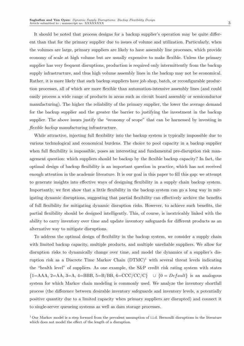
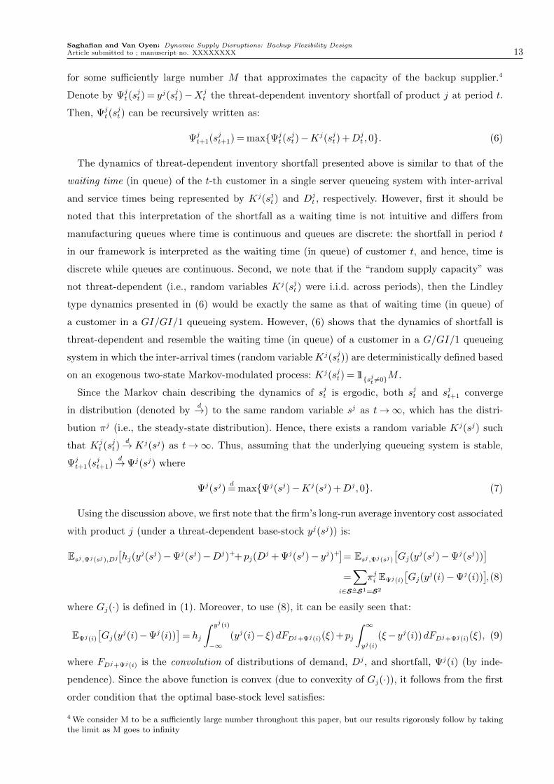
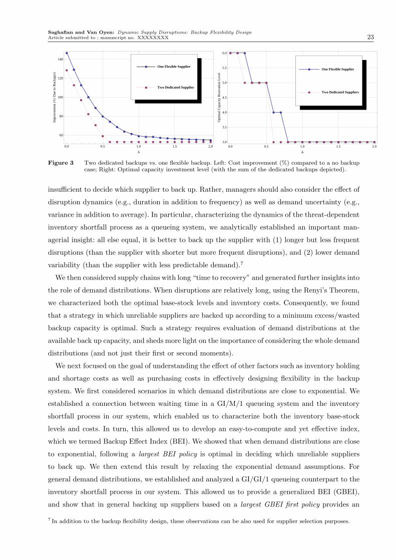
Fig. 3 (left) reveals the insight that the value of the fully flexible backup supplier is more than the

summation of benefits that can be obtained separately for each of the products through dedicated

backups (assuming that the dedicated backup suppliers are priced similar to the flexible backup

one). This is mainly due to the capacity pooling advantage of the flexible backup supplier; when

one of the primary suppliers is in a high risk threat level and the other is in a low threat level, the

reserved pooled capacity can be used as needed. However, using the difference between the two

curves depicted in Fig. 3 (left), we can make the following observation.

Observation 2. The pooling advantage is not monotone in ∆ and has its maximum effect when ∆

is in a middle range. However, as ∆ increases, the pooling advantage vanishes: the backup flexible

supplier can only be used for a single product, performing as a dedicated backup supplier.

Fig. 3 (right) depicts the corresponding optimal investment levels in the backup suppliers. From

this figure we observe the following.

Observation 3. The sum of optimal capacities required for product 1 and 2 in the case of two

dedicated backup suppliers is never larger than the optimal capacity for the flexible backup supplier.

The observation above highlights the justification for higher levels of investments (or capacity

reservation) fees charged in practice by flexible suppliers.

7. Summary of Findings and Concluding Remarks

We investigated the optimal design of flexibility in the backup system as a potent supply risk

mitigation mechanisms. Analogous to some models for credit risk rating systems (e.g., S&P), we

modeled the dynamics of disruptions as discrete time Markov chains, and considered a multi-

product, multi-supplier supply chain under dynamically evolving disruption risks.

We analytically showed the important insight that in mitigating dynamic disruptions “a little

backup flexibility can go a long way.” When suppliers are asymmetric and full flexibility is not pos-

sible (or is too expensive) this raises a fundamental question: which unreliable supplier(s) should

be backed up? We addressed this question and observed that focusing merely on the first moment

effects such as average demand (product popularity) or suppliers’ reliability (percentage uptime) is

Saghafian and Van Oyen: Dynamic Supply Disruptions: Backup Flexibility DesignArticle submitted to ; manuscript no. XXXXXXXX 23

æ

æ

æ

æ

æ

æ

æ

æ

æ

æ

æ æ ææ æ æ æ æ æ æ æ

à

à

à

à

à

à

à à à à à à à à à à à à à à à

0.0 0.5 1.0 1.5 2.0

60

80

100

120

140

D

Impr

ovem

entH

%LD

ueto

Bac

kupHs

L

à Two Dedicated Suppliers

æ One Flexible Supplier

æ æ æ

æ æ æ

æ æ

æ æ æ æ æ æ æ æ æ æ æ æ æ

à à

à à à à

à à à à à à à à à à à à à à à

0.0 0.5 1.0 1.5 2.03.0

3.5

4.0

4.5

5.0

5.5

6.0

D

Opt

imal

Cap

acity

Res

evat

ion

Lev

el

à Two Dedicated Suppliers

æ One Flexible Supplier

Figure 3 Two dedicated backups vs. one flexible backup. Left: Cost improvement (%) compared to a no backupcase; Right: Optimal capacity investment level (with the sum of the dedicated backups depicted).

insufficient to decide which supplier to back up. Rather, managers should also consider the effect of

disruption dynamics (e.g., duration in addition to frequency) as well as demand uncertainty (e.g.,

variance in addition to average). In particular, characterizing the dynamics of the threat-dependent

inventory shortfall process as a queueing system, we analytically established an important man-

agerial insight: all else equal, it is better to back up the supplier with (1) longer but less frequent

disruptions (than the supplier with shorter but more frequent disruptions), and (2) lower demand

variability (than the supplier with less predictable demand).7

We then considered supply chains with long “time to recovery” and generated further insights into

the role of demand distributions. When disruptions are relatively long, using the Renyi’s Theorem,

we characterized both the optimal base-stock levels and inventory costs. Consequently, we found

that a strategy in which unreliable suppliers are backed up according to a minimum excess/wasted

backup capacity is optimal. Such a strategy requires evaluation of demand distributions at the

available back up capacity, and sheds more light on the importance of considering the whole demand

distributions (and not just their first or second moments).

We next focused on the goal of understanding the effect of other factors such as inventory holding

and shortage costs as well as purchasing costs in effectively designing flexibility in the backup

system. We first considered scenarios in which demand distributions are close to exponential. We

established a connection between waiting time in a GI/M/1 queueing system and the inventory

shortfall process in our system, which enabled us to characterize both the inventory base-stock

levels and costs. In turn, this allowed us to develop an easy-to-compute and yet effective index,

which we termed Backup Effect Index (BEI). We showed that when demand distributions are close

to exponential, following a largest BEI policy is optimal in deciding which unreliable suppliers

to back up. We then extend this result by relaxing the exponential demand assumptions. For

general demand distributions, we established and analyzed a GI/GI/1 queueing counterpart to the

inventory shortfall process in our system. This allowed us to provide a generalized BEI (GBEI),

and show that in general backing up suppliers based on a largest GBEI first policy provides an

7 In addition to the backup flexibility design, these observations can be also used for supplier selection purposes.

Saghafian and Van Oyen: Dynamic Supply Disruptions: Backup Flexibility Design24 Article submitted to ; manuscript no. XXXXXXXX

effective backup flexibility design. Our indices (BEI and GBEI) provide supply chain designers with

easy-to-compute tools to decide which unreliable suppliers to backup, enabling them to effectively

compensate for dynamic disruption risks.

Finally, we explored the backup capacity pooling advantage by comparing dedicated backups

versus a pooled (i.e., fully flexible) backup capacity in a numerical study. We found that the value of

a flexible backup supplier is more than the summation of benefits that can be obtained separately

for each of the products through dedicated backups. Furthermore, a firm will reserve at least as

much capacity from a backup flexible supplier as the amount reserved in total from dedicated

backup ones. Indeed, the flexibility of a supplier provides the firm with greater benefits, justifying

reserving more backup capacity because of the economic advantage of shifting the orders whenever

necessary (capacity pooling). This observation also justifies flexible suppliers charging higher fees

for reserving their capacity compared to inflexible suppliers.

The analyses, modeling framework, and insights presented in this paper can guide new practices

to effectively increase the resilience of supply chains. Increasing the resilience of supply chains can

in turn enable firms to deliver products with better availability and better prices to end customers,

yielding social benefits. While this study focused on the cost to a firm, a fruitful path for future

research is to examine the possibility of creating such broader social advantages. Moreover, future

research may expand this study to consider issues such as risk aversion or potential correlations

between the dynamic disruption risks of different suppliers.

Acknowledgement. This work was supported in part by the National Science Foundation Grant CMMI 1068638,

and Office of Naval Research Grant N00014-08-1-0579. The authors sincerely thank Brian Tomlin, Wallace Hopp,

Xiuli Chao, Area Editor, Prof. Chung Piaw Teo, and the anonymous AE and referees for their invaluable comments

and insightful discussions which significantly improved the paper. The authors are also grateful to David Singer for

his support through the above ONR grant.

ReferencesAbate, J., G.L. Choudhury, W. Whitt. 1995. Exponential approximations for tail probabilities in queues, I: Waiting

times. Oper. Res., 43 (5), 885–901.Agrawal, N., S. Nahmias. 1997. Rationalization of the supplier base in the presence of yield uncertainty. Prod. andOper. Man., 6, 291–308.

Anupindi, R., R. Akella. 1993. Diversification under supply uncertainty. Management Sci., 39(8), 944–963.Arreola-Risa, A., G.A. DeCroix. 1998. Inventory management under random disruptions and partial back-orders. NavalRes. Logist., 45, 687-703.

Babich, V., A.N. Burnetas, P.H. Ritchken. 2007. Competition and diversification effects in supply chains with supplierdefault risk, Manufacturing & Service Oper. Management, 9 (2), 123–146.

Bassamboo, A, R.S. Randhawa, J.A. Van Mieghem . 2010 Optimal flexibility configurations in newsvendor networks:Going beyond chaining and pairing. Management Sci., 56, 1285–1303.

Behdani, B., A. Adhitya, Z. Lukszo, R. Srinivasan. 2012. How to Handle Disruptions in Supply Chains An IntegratedFramework and a Review of Literature, Working Paper, Delft University of Technology.

Blanchet, J., P. Glynn. 2007. Unified renewal theory with applications to expansions of random geometric sums. Adv.Appl. Prob., 39, 1070–1097.

Bollapragada, R., U.S. Rao, J. Zhang. 2004. Managing inventory and supply performance in assembly systems withrandom supply capacity and demand. Management Sci., 50, 1729-1743.

Brown, A.P., H.L. Lee, 1997. Optimal pay to delay capacity reservation with applications to the semiconductor industry.Working Paper, Stanford University.

Business Continuity Institute, 2011. Supply Chain Resilience, 3rd Annual Survey.Cho, S.H., C.S. Tang, 2011. Advance selling in a supply chain under uncertain supply and demand, Working Paper,

Saghafian and Van Oyen: Dynamic Supply Disruptions: Backup Flexibility DesignArticle submitted to ; manuscript no. XXXXXXXX 25

Carnegie Mellon University.Chou, M.C., G.A. Chua, H. Zheng, C.-P. Teo, 2010. Design for process flexibility: Efficiency of the long chain andsparse structure. Oper. Res. 58(1) 43–58.

Ciarallo, F. W., R. Akella, T.E., Morton. 1994. A periodic review, production planning model with uncertain capacityand uncertain demand: Optimality of extended myopic policies. Management Sci., 40, 320–332.

Cohen, S., R. Geissbauer, A. Bhandari, M. Dheur. 2008. Global supply chain trends 2008–2010: Driving global supplychain flexibility through innovation. Survey, PRTM Management Consultants, Washington, DC.

Daley, D.J. 1968. Stochastically monotone Markov Chains. Probability Theory and Related Fields 10 (4), 305–317.Dawson, C. 2011. Quake Still Rattles Suppliers. The Wall Street Journal, Sept. 29.DeCroix, G.A., A. Arreola-Risa 1998. Optimal production and inventory policy for multiple products under resource

constraints, Management Sci., 44, 950–961.Dong, L, B. Tomlin 2012. Managing disruption risks: The interplay between operations and insurance. ManagementSci. (forthcoming).

Erdem, A. 1999. Inventory models with random yield. Ph.D. dissertation (Chapter 4).Fedegruen, A., N. Yang 2009. Competition under generalized attraction models: Applications to quality competition

under yield uncertainty, Management Sci., 55(12), 2028–2043.Gerchak, Y., M. Parlar. 1990. Yield randomness, cost trade-offs and diversification in the EOQ model. Naval Res.Logist. 37, 341–354.

Glasserman, P., 1997. Bounds and Asymptotics For Planning Critical Safety Stocks. Oper. Res., 45(2), 244-257.Graves, S.C., B.T. Tomlin. 2003. Process flexibility in supply chains. Management Sci., 49, 907–919.Greising, D., J. Johnsson. 2007. Behind Boeing 787 delays: problems at one of the smallest suppliers in Dreamlinerprogram causing ripple effect. Chicago Tribune, December, 08.

Gurler, U., M. Parlar. 1997. An inventory problem with two randomly available suppliers. Oper. Res., 45, 904–918.Gurnani, H., R. Akella, J. Lehoczky. 2000. Supply management in assembly systems with random yield and random

demand. IIE Trans., 32, 701–714.Henig, M., Y. Gerchak. 1990. The structure of periodic review policies in the presence of random yield. Oper. Res., 38,

634–643.Hopp, W.J., E. Tekin, M.P. Van Oyen. 2004. Benefits of skill chaining in production lines with cross-trained workers.Management Sci. 50(1) 83–98.

Hopp, W.J., M.P. Van Oyen. 2004. Agile workforce evaluation: A framework for cross-training and coordination. IIETrans. 36(10) 919–940.

Iravani, S.M., M.P. Van Oyen, K.T. Sims. 2005. Structural flexibility: A new perspective on the design of manufacturingand service operations. Management Sci., 51, 151–166

Iravani, S.M., B. Kolfal, M.P. Van Oyen. 2011. Capability flexibility: A decision support methodology for productionand service systems with flexible resources. IIE Trans., 43, 363-382.

Jordan, W.C., S.C. Graves. 1995. Principles on the benefits of manufacturing flexibility. Management Sci., 41, 577–594.Kim, C.R. 2011. Toyota aims for quake-proof supply chain. Reuters, Sep. 06.Kingman, J.F.C. (1964) A martingale inequality in the theory of queues. Proc. Camb. Phil. Soc. 59, 359–361.Kingman, J.F.C. (1970) Inequalities in the theory of queues. J. R. Statist. Soc. B 32, 102–110.Kleinrock, L. 1975. Queueing Systems: Theory (Volume 1), Wiley.

Kouvelis, P., J. Li. 2008. Flexible Backup Supply andthe Management of Lead-Time Uncertainty.Prod. and Oper.Management, 17:2, 184-199.

Kouvelis, P., G. Vairaktarakis. 1998. Flowshops with processing flexibility across production stages. IIE Trans. 30,735–746.

Moinzadeh, K., P. Aggarwal. 1997. Analysis of a production/inventory system subject to random disruptions. Man-agement Sci., 43, 1577–1588.

Norrman, A., U. Jansson. 2004. Ericsson’s proactive supply chain risk management approach after a serious sub-supplieraccident. International J. of Phys. Dist. and Log. Management, 34:5, 434-456.

Ozekici, S., M. Parlar. 1999. Inventory models with unreliable suppliers in random environment. Annals of Oper. Res.,91, 123-136.

Parlar, M., D. Perry. 1996. Inventory models of future supply uncertainty with single and multiple suppliers. NavalRes. Logist., 43, 191-210.

Parlar, M., Y. Wang, Y. Gerchak. 1995. A periodic review inventory model with Markovian supply availability. Internat.J. Prod. Economics, 42, 131136.

Prabhu, N.U. 1965. Queues and Inventories, Wiley.Reitman, V. 1997. Toyota Motor shows its mettle after fire destroys parts plant. The Wall Street Journal, May, 08)Ross, S.M. 1974. Bounds on the delay distribution in GI/G/1 queues, J. Appl Prob., 11 (2), 417–421.Saghafian, S., M.P. Van Oyen, 2011. The “W” network and the dynamic control of unreliable flexible servers. IIETrans., 43 (12), 893–907.

Saghafian, S., M.P. Van Oyen, 2012. The value of flexible suppliers and disruption risk information: Newsvendoranalysis with recourse. IIE Trans., 44 (10), 834–867.

Serel, D.A., M. Dada, H. Moskowitz. 2001. Sourcing decision with capacity reservation contract. Eur. J. Oper. Res.,131, 635–648.

Shaked, M, J.G. Shanthikumar. 2007. Stochastic Orders, Springer.

Saghafian and Van Oyen: Dynamic Supply Disruptions: Backup Flexibility Design26 Article submitted to ; manuscript no. XXXXXXXX

Sheffi, Y. 2007. The resilient enterprise: overcoming vulnerability for competitive advantage, The MIT Press, Cam-bridge, Massachusetts.

Simchi-Levi, D., W. Schmidt, Y. Wei. 2014. From superstorms to factory fires: Managing unpredictable supply-chaindisruptions. Harvard Bus. Rev., (JanuaryFebruary) 96–101.

Simchi-Levi, D., H. Wang, Y. Wei. 2013. Increasing supply chain robustness through process flexibility and strategicinventory. Working paper, Massachusetts Institute of Technology.

Simchi-Levi, D., Y. Wei. 2012. Understanding the performance of the long chain and sparse designs in process flexibility.Oper. Res., 60, 1125 - 1141.

Song, J-S., P.H. Zipkin. 1996. Inventory control with information about supply conditions. Management Sci. 42,1411–1419.

Swaminathan, J.M., J.G. Shanthikumar. 1999. Supplier diversification: effect of discrete demand. Oper. Res. Let., 24(5)213–221.

Swinney, R., S. Netessine. 2009. Long-term contracts under the threat of supplier default. Manufacturing Service Oper.Management, 11, 109–127.

Tang, C.S. (2006) Robust strategies for mitigating supply chain disruptions, Inter. J. of Log. Res. and Appl.. 9(1),33–45.

Tayur, S. R. 1993. Computing The Optimal Policy For Capacitated Inventory Models. Comun. Statist., 9, 585-598.Tomlin, B. 2006. On the value of mitigation and contingency strategies for managing supply-chain disruption risks.Management Sci., 52(5), 639–657.

Tomlin, B., C.S., Tang. 2008. The power of flexibility for mitigating supply chain risk. Inter. J. of Prod. Econ., 116(1), 12–17.

Tomlin, B. 2009. The impact of supply-learning on a firms sourcing strategy and inventory investment when suppliersare unreliable. Manufacturing Service Oper. Man., 11, 192–209.

Tomlin, B., L., Snyder. 2006. On the value of a threat advisory system for managing supply chain disruptions. Workingpaper, University of North Carolina Chapel Hill.

Tomlin, B., Y. Wang. 2005. On the value of mix flexibility and dual sourcing in unreliable newsvendor networks.Manufacturing Service Oper. Man., 7, 37-57.

Van Mieghem, J.A. 1998. Investment strategies for flexible resources. Management Sci., 44, 1071–1078.Wang, Y., W., Gilland, B., Tomlin. 2010. Mitigating supply risk: dual sourcing or process improvement?, ManufacturingService Oper. Man., 12 (3), 489-510

Yano, C. A., H.L. Lee. 1995. Lot sizing with random yield: A review. Oper. Res., 43, 311–334.