Competition and Consumer Confusion

Xavier Gabaix

MIT and NBER

David Laibson

Harvard University and NBER

Current Draft: April 30, 2004∗

Abstract

In many markets consumer biases do not affect prices, since competition forces firms to price

their products close to marginal cost; competition protects the consumer. We show that noisy

consumer product evaluations undermine the force of competition, enabling firms to charge

high mark-ups in equilibrium, even in highly competitive environments. We analyze markets in

which rational firms sell goods to consumers who evaluate products with noise. Using results

from extreme value theory, we show that competition generally has a remarkably weak impact

on markups. For normally distributed evaluation noise, we show that markups are proportional

to the inverse of√lnn, where n is the number of competitors. In this setting, a highly compet-

itive industry with n = 1, 000, 000 firms will retain 1/3 of the markup of a highly concentrated

industry with only n = 10 competitors. When we make noise an endogenous variable, we find

that firms choose excess noise by making their products inefficiently confusing. Moreover, com-

petition exacerbates this effect: a higher degree of competition causes firms to choose even more

excess complexity. Firms with lower intrinsic quality and higher production costs choose the

most excess complexity. Educating consumers to reduce their evaluation noise would generate

∗For useful suggestions we thank Simon Anderson, Roland Bénabou, Douglas Berheim, Andrew Caplin,Victor Chernozhukov, Casper de Vries, Avinash Dixit, Edward Glaeser, Penny Goldberg, Robert Hall,Sergei Izmalkov, Julie Mortimer, Barry Nalebuff, Aviv Nevo, Nancy Rose, José Scheinkman, Andrei Shleifer,Wei Xiong and seminar participants at Berkeley, Columbia, Harvard, MIT, NBER, New York University,Princeton, Virginia, the 2003 European Econometric Society meeting, the 2003 SITE meeting, and the 2004AEA meeting. We acknowledge financial support from the NSF (SES-0099025). Gabaix thanks the RussellSage Foundation for their hospitality during the year 2002-3. Xavier Gabaix: MIT, 50 Memorial Drive,Cambridge, MA 02142, xgabaix@mit.edu. David Laibson: Harvard University, Department of Economics,Cambridge, MA, 02138, dlaibson@arrow.fas.harvard.edu.

1

large welfare gains. But the gains accrue mostly to the consumer, so firms can’t profitably ed-

ucate consumers and steal them away from competitors. Finally, we introduce an econometric

framework that measures bounded rationality and confusion in the marketplace.

JEL classification: D00, D80, L00.

Keywords: bounded rationality, complexity, confusion, extreme value theory, discrete

choice, profit, behavioral economics, behavioral industrial organization, mutual fund

industry, consumer protection.

2

1 Introduction

In standard markets competition protects consumers from their own cognitive biases. For example,

even if consumers overweight small probability events1 and overestimate the value of life insurance,

the equilibrium price of life insurance will still equal marginal cost. Cognitive errors do not

affect the price since competing life insurance companies will undercut each other until price equals

marginal cost.

We study a small perturbation to the traditional economic approach and find that it makes

competition lose most of this price-cutting force. When consumers have noisy product evaluations,

firms have market power that barely decreases as competition rises. We represent a consumer’s

ex-ante estimate of the value of a good as the sum of the (true) expected consumption value plus

evaluation noise. Assuming that consumers have noisy beliefs doesn’t seem like a very strong

assumption. Mutual fund investors, for instance, don’t know the expense ratios of the funds they

buy (Alexander et al 1998, Barber et al. 2002). Desktop printer buyers don’t know the cost of ink

per page (Hall 1997). Wine store customers – like the second author of this paper – don’t know

the difference between Gamay and Grenache. Wine may be an example of a good with extremely

noisy in-store evaluations, but almost every good gets sized up with at least a little noise.

We analyze markets in which there are many perfectly rational firms selling goods to consumers

that have noisy product evaluations. The paper can be divided into an analysis of five questions

about those markets.

First, we ask whether firms will exploit the noisy consumer evaluations. Following Perloff and

Salop (1985), we find that equilibrium markups are proportional to the amount of noise. Higher

levels of noise increases the chance that a consumer will either overestimate or underestimate the

surplus associated with the firm’s good. Firms take advantage of this noise by raising their

prices. Such price increases reflect the fact that noise reduces the sensitivity of consumers to small

differences in product attributes. This in turn reduces the elasticity of each firm’s demand curve,

leading firms to raise equilibrium prices.

Second, we ask how increased competition affects markups. Using results from extreme value

theory, we find that competition typically has remarkably little impact on markups. Our leading

1See Kahneman and Tversky (1979).

3

example is the case of normally distributed noise. For this case, we show that markups are propor-

tional to³√lnn

´−1, where n is the number of competitors.2 A highly competitive industry with

n = 1, 000, 000 firms will have 1/3 the markup of an industry with only n = 10 competitors. When

consumers have typical (thin-tailed) noise distributions, competition – even extreme competition

– barely reduces markups. Moreover, we show that competition actually increases markups when

consumers have fat-tailed distributions.

Third, we ask how firms will manipulate the amount of noise when they are able to do so.

In this analysis, complexity is itself an endogenous variable chosen by each firm. For example,

a firm can create an unnecessarily complex fee schedule, which makes it harder for a consumer

to determine the true cost of the good. We show that firms will generally prefer such excess

complexity. A small amount of excess complexity has only a second-order negative impact on the

intrinsic quality of the good, but generates a first order increase in the (confusion-driven) demand

for the good. So firms choose inefficiently high levels of complexity.

Fourth, we ask what determines a firm’s choice of excess complexity. We show that higher levels

of competition increase the equilibrium amount of excess complexity. Firms in highly competitive

markets have small market shares and have more to gain from excess complexity. We also show

that firms with higher intrinsic quality and lower production costs choose less excess complexity.

Intuitively, high quality firms maximize profits by making their competitive advantage relatively

transparent (i.e., they reduce noise). By contrast, average or high cost firms will pick a high degree

of complexity, maximizing profits by taking advantage of the fact that their over-priced product

will be misevaluated by some fraction of consumers.

Fifth, we ask whether firms have an incentive to educate consumers and thereby turn naive con-

sumers (with noisy product evaluations) into sophisticated consumers (with less noisy evaluations).

We show that such incentives are quite weak, since sophisticated consumers are much less profitable

to firms than naive consumers. The large gains from education disproportionately accrue to the

consumer, generating a wedge that makes it impossible for firms to profitably educate consumers

and thereby steal them away from other firms.

We also introduce an econometric framework that can be used to measure bounded rationality

2Hence, mark-ups converge very slowly to zero with n. This is by contrast with the Cournot model in whichmarkets are proportional to 1/n.

4

and confusion in the marketplace. The model exploits the fact that populations of consumers

with identical underlying objective functions should consume similar bundles of goods. When

otherwise identical sophisticated and naive consumers buy different bundles of goods, then the

naive consumers suffer from some confusion about the goods they are buying. We introduce

an econometric framework that can measure such effects by exploiting randomized educational

interventions.

The rest of this paper formalizes these claims. Section 2 describes the general model where con-

sumers have noisy signals about product value and firms can control the level of noise. Section 3

shows that the existence of noise increases firms’ market power and that competition does remark-

ably little to offset these effects. Section 4 shows that firms have an incentive to generate excess

complexity, and that excess complexity increases with the amount of competition and decreases

with product quality. Section 5 explains why firms won’t educate consumers. Section 6 describes

a practical econometric framework for measuring the magnitude of confusion. Section 7 concludes.

Before proceeding, we start with a review of the literature. We show how the market power

coming from bounded rationality differs from market power coming from search costs and hetero-

geneous tastes, both for positive and normative analysis. Of course, all three (and more) sources

of market power coexist in most markets.

Literature Review Since its inception in the late 1970’s, psychological principles have been

applied in every traditional field of economics. Our paper contributes to the emergent field of

behavioral industrial organization3 (DellaVigna and Malmendier 2003 and Oster and Morton 2004

apply hyperbolic discounting; Heidhues and Koszegi 2004 and Koszegi and Rabin 2004 apply loss

aversion; Gabaix and Laibson 2004 and Spiegler 2003 apply boundedly rational heuristics).

Our paper is partially motivated by empirical work that suggests that consumers are sometimes

confused about the decisions that they make. Woodward (2003) documents confusion in the

mortgage market, which decreases with the level of household education. Madrian and Shea (2002)

and Choi et al (2003a, 2003b) show that workers are extraordinarily sensitive to the defaults in their

401(k) plan (e.g., automatic enrollment), suggesting that consumers do not have a clear model of

3The first papers in “behavioral IO” may be Hausman (1979) and Hausman and Joskow (1982), who find that fordurables consumers seem to care more about upfront costs that future flow costs.

5

how to invest for retirement. Benartzi and Thaler (2001, 2002) show that investors allocate their

financial assets noisily. For example, Benartzi and Thaler (2002) find that the 401(k) investors

choose a mix of stocks and bonds that is driven by the proportion of stock funds available in the

investor’s 401(k) plan. Asset allocation appears to derive at least partially from randomization

over the set of available funds.

Our model is motivated by the standard Luce (1959)-McFadden (1981) random utility frame-

work, (see Anderson, de Palma and Thisse 1992 for a review of this literature and Sheshinski 2003

for a recent implementation). We extend the markup calculations of Perloff and Salop (1985).

Like the previous literature, our analysis uses extreme value theory. Analytic markup calculations

for Gumbel noise (Anderson et al 1992) and exponential noise (Perloff and Salop 1985) were already

known. We derive asymptotic approximations for a much wider class of distributions, including

Gaussian, exponential, log-normal, and power-law densities. Our results for endogenous noise are

also original. We extend previous analyses interpreting this noise as a form of bounded rationality

(Anderson et al. 1998, McFadden 1981, De Palma et al. 1994, Sheshinksi 2003). A related IO

literature analyzes rational (Bayesian) consumers who have noisy product evaluations (Judd and

Riordan 1994 and Anantham and Ben-Shoham 2004).

Our work is related to the literature on advertising (e.g. Becker and Murphy 1990, Dixit

and Norman 1978; see Bagwell 2002 for a remarkable review of the advertising literature). We

believe that advertising and marketing play a key role in generating the noise in consumer product

evaluations. Consumers have a hard time filtering misleading marketing signals about goods.

Imperfect (but unbiased) filters will create noisy impressions about product value.

Our paper is also related to the literature on search (e.g., Stigler 1961, Diamond 1971, Salop

and Stiglitz 1977). Like search models, our model predicts that consumers will not always purchase

the most competitively priced good. However, our framework has little else in common with the

search framework. Our model has a different microfoundation and explores different phenomena:

e.g., endogenous market power arising from endogenous noise.

6

2 General Model with Complexity

2.1 Consumers

Our model is motivated by the standard Luce (1959)-McFadden (1981) random utility framework.4

Each consumer must pick one good from a set of n goods. For consumer a, good i has complexity

σi, value vi, and price pi. Consumers do not directly observe either σi, vi, or pi. Instead, consumer

(agent) a observes only a noisy signal of good i’s net value, where the noise component scales with

the complexity of the good.

Uia = vi − pi| {z } + σiεia| {z }true value noise

.

The scaled noise term, σiεia, captures consumer a’s noise in evaluating product i. We assume that

εia is zero mean5 and i.i.d. across consumers and goods. Let εia have unit variance, density f,

cumulative distribution F , and ‘complexity’ scaling factor σi.

These assumptions imply that before consumers purchase a good, the consumers do not know

the true expected value or the true expected cost of the good. This imperfect observability may

arise for many possible reasons. Marketing campaigns create noise. Mental simulations of the

future use value create noise. Indeed, all complex mental calculations are associated with error.

Costs are also perceived with noise, since the sticker price is often not the end of the cost story.

Many goods have complex repair costs or other add-on costs. Durables have complex financing

arrangements.

We summarize the consumer’s noisy evaluations of both value and price by assuming that

consumer a only observes a utility signal Uia for each good and does not observe its constituent

components. We assume that the consumer uses a very simple and sensible decision-rule: pick the

good with the highest signal value. So consumer a chooses the firm i with the highest value of

Uia.6 In our baseline model, this sensible heuristic rule will also be an optimal policy.7

4See Anderson, de Palma and Thisse (1992) for an excellent review of this literature.5 In the leading cases, the mean of the noise does not matter for the equilibrium. In particular, the mean does not

matter when firms have identical noise intensity, σi.6We assume that the consumer must have (and will buy) exactly one good, even if the largest Uia is negative for

consumer a.7Appendix C offers a class of situations where this is the optimal rule, and discusses how the conclusions of our

model change in other cases.

7

To simplify notation, we suppress the consumer specific subscript a for the rest of the paper,

so Ui ≡ Uia and εi ≡ εia unless otherwise noted.

2.2 Firms

Each firm needs to pick an endogenous price, pi, and a level of product complexity, σi. We assume

that changes in complexity, σi, have two effects. Product complexity influences the underlying

intrinsic valuation of the product, so vi = v(σi). Second, product complexity influences the standard

deviation of the noise that will be perceived by the consumers (cf. subsection 2.1).

If a social planner designed goods and assigned them to consumers, such efficient products

would typically have a level of complexity σ > 0. For example, an efficient computer will trade

off the costs of complexity – e.g. “It’s so complex that I can’t figure out how to use it.” – with

the benefits of complexity – e.g. “The computer can be used to do many different things.” If a

product is too complex it will be inefficiently too hard to use, but if a product is too simple it will

have inefficiently too few features.

We capture these trade-offs by assuming that complexity σ gives rise to a hump-shaped valuation

function v (σ). Figure 1 presents an example of such a function. There is a maximum at σ∗ ≥ 0,the “bliss point” for complexity.

We study the Bertrand equilibrium with endogenous complexity, where firms maximize profit,

πi, by choosing (pi, σi):

maxpi,σi

πi ≡ (pi − c)D (pi, σi) , (1)

where c is the marginal cost of production and D is the firm’s demand function. In a symmetric

equilibrium, the demand function of firm i is equal to the probability that a consumer receives the

best noisy signal from firm i, so

D (pi, σi) = P

µv (σi)− pi + σiεi > max

j 6=iv (σ)− p+ σεj

¶= P

µv (σi)− pi − [v (σ)− p] + σiεi > max

j 6=iσεj

¶.

It is convenient to rewrite the firm’s maximization problem by introducing a change of variables.

Define a new demand function D that takes as its first argument the intrinsic surplus x of firm i

8

relative to its competitors,

D (x, σi) ≡ P

µx+ σiεi > max

j 6=iσεj

¶. (2)

Define

xi ≡ v (σi)− pi − [v (σ)− p] . (3)

Now the firm’s optimization problem may be rewritten

maxxi,σi

(pi(xi, σi)− c)D (xi, σi) ,

where pi(xi, σi) is defined by rearranging equation (3),

pi(xi, σi) ≡ v (σi)− xi − [v (σ)− p] . (4)

Call

Mn−1 = maxj∈{1,...,n},j 6=i

εi, (5)

so Mn−1 is the highest of n− 1 noise realizations. Then,

D (x, σi) = P

µεi >

−x+ σMn−1σi

¶D (x, σi) = E

·F

µ−x+ σMn−1σi

¶¸, (6)

where F (x) =R∞x f (y) dy is the countercumulative distribution function. This formulation em-

phasizes the property that the demand for good i is driven by the right-hand tail properties of the

countercumulative distribution function, F.

The properties of the symmetric equilibrium8 can be derived from the behavior of D (x, σi) at

(x, σi) = (0, σ). Specifically, (6) gives:

8Section 9.9 treats the existence of the symmetrical equilibrium.

9

∂

∂xD (0, σ) =

1

σE [f (Mn−1)] (7)

∂

∂σiD (0, σ) =

1

σE [f (Mn−1)Mn−1] (8)

D (0, σ) =1

n. (9)

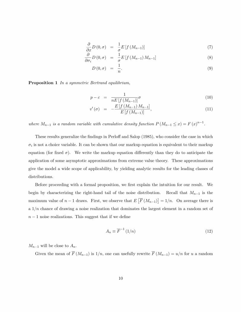
Proposition 1 In a symmetric Bertrand equilibrium,

p− c =1

nE [f (Mn−1)]σ (10)

v0 (σ) = −E [f (Mn−1)Mn−1]E [f (Mn−1)]

, (11)

where Mn−1 is a random variable with cumulative density function P (Mn−1 ≤ x) = F (x)n−1.

These results generalize the findings in Perloff and Salop (1985), who consider the case in which

σi is not a choice variable. It can be shown that our markup equation is equivalent to their markup

equation (for fixed σ). We write the markup equation differently than they do to anticipate the

application of some asymptotic approximations from extreme value theory. These approximations

give the model a wide scope of applicability, by yielding analytic results for the leading classes of

distributions.

Before proceeding with a formal proposition, we first explain the intuition for our result. We

begin by characterizing the right-hand tail of the noise distribution. Recall that Mn−1 is the

maximum value of n− 1 draws. First, we observe that E £F (Mn−1)¤= 1/n. On average there is

a 1/n chance of drawing a noise realization that dominates the largest element in a random set of

n− 1 noise realizations. This suggest that if we define

An ≡ F−1(1/n) (12)

Mn−1 will be close to An.

Given the mean of F (Mn−1) is 1/n, one can usefully rewrite F (Mn−1) = u/n for u a random

10

variable near 1. We therefore expand Mn−1 = F−1 ¡u

n

¢around u = 1.

Mn−1 = F−1 ³u

n

´' F

−1µ1

n

¶+³F−1´0µ 1

n

¶u− 1n

= An − 1

f (An)

u− 1n

.

So the dispersion in Mn−1 is the dispersion of 1f(An)

u−1n , which implies that variation in Mn−1 is

proportional to 1/ [nf (An)]. We conclude that the typical difference between the best draw and

the second best draw is proportional to 1/ [nf (An)]. Using standard optimization arguments, a

firm sets its markup proportional to this dispersion, so that p− c ∼ 1/ [nf (An)].

The following Proposition shows that this heuristic argument generates the right approximation

for the Gaussian, exponential, Gumbel and lognormal distributions. The Proposition also shows

that the approximation remains accurate up to a corrective constant Γ (2 + ξ) in other cases.

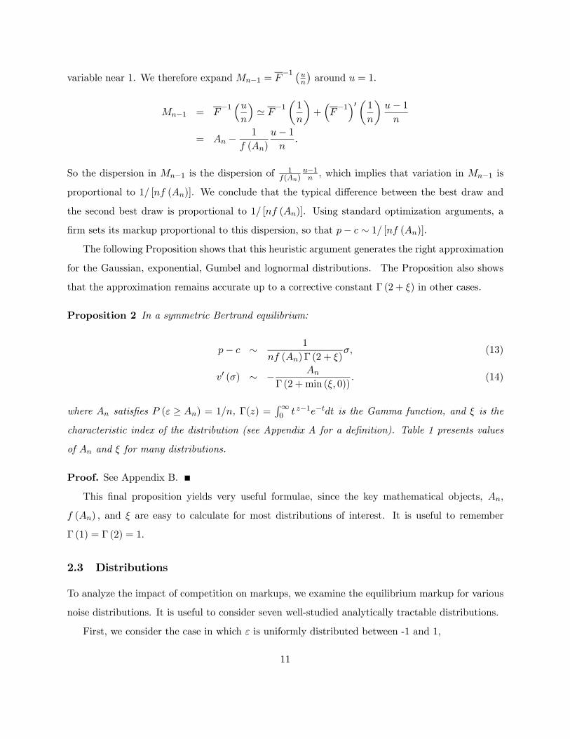
Proposition 2 In a symmetric Bertrand equilibrium:

p− c ∼ 1

nf (An)Γ (2 + ξ)σ, (13)

v0 (σ) ∼ − An

Γ (2 + min (ξ, 0)). (14)

where An satisfies P (ε ≥ An) = 1/n, Γ(z) =R∞0 t z−1e−tdt is the Gamma function, and ξ is the

characteristic index of the distribution (see Appendix A for a definition). Table 1 presents values

of An and ξ for many distributions.

Proof. See Appendix B.

This final proposition yields very useful formulae, since the key mathematical objects, An,

f (An) , and ξ are easy to calculate for most distributions of interest. It is useful to remember

Γ (1) = Γ (2) = 1.

2.3 Distributions

To analyze the impact of competition on markups, we examine the equilibrium markup for various

noise distributions. It is useful to consider seven well-studied analytically tractable distributions.

First, we consider the case in which ε is uniformly distributed between -1 and 1,

11

fUniform (ε) =1

21|ε|<1. (15)

which generalizes to a density in [−1, 1] that is power law around ε = 1−,

fBounded power law (ε) ∼ αk−α (1− ε)α−1 , (16)

with α > 0. For a large number of firms, only the right tail matters. So it is enough to characterize

the behavior of the density near the right boundary.

We also consider the Gaussian density,

fGaussian (ε) =1√2π

e−ε2/2, (17)

the Gumbel density (where θ ' 0.577216 is Euler’s constant),

fGumbel (ε) = exp³−e−ε−θ − ε− θ

´, (18)

the exponential density,

fExponential (ε) = e−(ε+1)1ε>−1, (19)

the log-normal density,

fLognormal (ε) =1

(ε+√e)√2π

e− ln(ε+√e)2/21ε>−√e, (20)

and the power law density for large ε,

fPower law ζ (ε) ∼ ζkζε−ζ−1. (21)

The shift factors θ, 1, and√e ensure that the mean of ε is 0 in each distribution. The densities

are ranked from thinnest to fattest tails.9

The reader may be uncomfortable with the use of unbounded noise distributions. But we

9A density g has fatter tails than a density f if there is a positive constant D such that for all x above a certainthreshold f (x) ≤ Dg (x).

12

use unbounded distributions only for analytical convenience, not because one needs to assume

that distributions are truly unbounded.10 Indeed, the results that follow will still hold if the

distribution of the noise is truncated on the right by some upper bound.11 We only fundamentally

need to evaluate the behavior of the noise density in the part of the right-hand-tail with cumulative

probability 1/n.

We calculate the Bertrand outcome for the seven distributions discussed above. Some of our

calculations are asymptotic expansions, which hold for large n and small positive t. Table 1

reports values for the key ingredients in our calculations.12 In this table, f is the density, F (x) ≡R∞x f (y) dy is the countercumulative function, An ≡ F

−1(1/n), h (t) ≡ f

³F−1(t)´, and ξ is the

characteristic index of F (i.e., an index of the fatness of the distribution, see Appendix A). For

application of Proposition (2), note that f (An) = h (1/n).

Table 1: Distributions and Associated Functions.An ≡ F

−1(1/n) h (t) ≡ f

³F−1(t)´

ξ

Uniform 1− 2/n 1/2 −1Bounded power law 1− kn−1/α + o

¡n−1/α

¢ ∼ αk−1t1−1/α −1/αGaussian ∼ √2 lnn ∼ t

q2 ln 1t 0

Gumbel ∼ lnn ∼ t 0

Exponential lnn− 1 t 0

Lognormal ∼ e√2 lnn ∼ te

−q2 ln 1

t+ 12ln(2 ln 1

t ) 0

Power law ∼ kn1/ζ ∼ ζk−1t1+1/ζ 1/ζ

Key quantities for Proposition 2.

10The same issues arise when economists model GDP growth as a Gaussian variable.11See Appendix B.12The proof is a consequence of e.g. Embrechts et al. (1997, p.155-7) and simple calculations.

13

3 Toothless competition

3.1 Will Competition Protect Consumers?

We now answer our second question: When consumers are confused, how do markups respond to

intensified competition? Naturally, the answer to this question depends on the distribution of the

noise in consumer evaluations. We assume that the standard deviation of noise, σ, is fixed and

focus analysis on endogenous markups and eventually endogenous entry. Proposition 3 provides

closed form expressions for the markups in different distributional cases for fixed σ and a fixed

number of competitors, n.

Proposition 3 The Bertrand equilibrium generates the following markups. For uniform noise

(15),

p− c =2

nσ. (22)

For bounded power law noise (16) with α > 1/2,

p− c ∼ k

αΓ (2− 1/α)n−1/ασ. (23)

For Gaussian noise (17),

p− c ∼ 1√2 lnn

σ. (24)

For Gumbel noise (18),

p− c =n

n− 1σ. (25)

For exponential noise (19),

p− c = σ. (26)

For log-normal noise (20),

p− c ∼ e√2 lnn− 1

2ln(2 lnn)σ. (27)

For power-law noise (21) with exponent ζ > 1,

p− c ∼ k

ζΓ (2 + 1/ζ)n1/ζσ. (28)

14

Proof. To obtain exact results we use equation (10) in Proposition 1. For approximate results we

use equation (13) in Proposition 2. We also exploit the distributional statistics in Table 1.

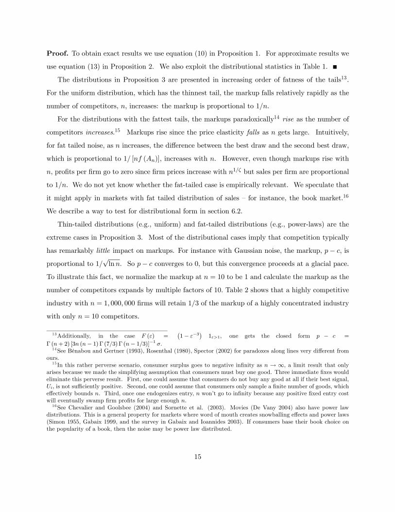
The distributions in Proposition 3 are presented in increasing order of fatness of the tails13.

For the uniform distribution, which has the thinnest tail, the markup falls relatively rapidly as the

number of competitors, n, increases: the markup is proportional to 1/n.

For the distributions with the fattest tails, the markups paradoxically14 rise as the number of

competitors increases.15 Markups rise since the price elasticity falls as n gets large. Intuitively,

for fat tailed noise, as n increases, the difference between the best draw and the second best draw,

which is proportional to 1/ [nf (An)], increases with n. However, even though markups rise with

n, profits per firm go to zero since firm prices increase with n1/ζ but sales per firm are proportional

to 1/n. We do not yet know whether the fat-tailed case is empirically relevant. We speculate that

it might apply in markets with fat tailed distribution of sales — for instance, the book market.16

We describe a way to test for distributional form in section 6.2.

Thin-tailed distributions (e.g., uniform) and fat-tailed distributions (e.g., power-laws) are the

extreme cases in Proposition 3. Most of the distributional cases imply that competition typically

has remarkably little impact on markups. For instance with Gaussian noise, the markup, p− c, is

proportional to 1/√lnn. So p− c converges to 0, but this convergence proceeds at a glacial pace.

To illustrate this fact, we normalize the markup at n = 10 to be 1 and calculate the markup as the

number of competitors expands by multiple factors of 10. Table 2 shows that a highly competitive

industry with n = 1, 000, 000 firms will retain 1/3 of the markup of a highly concentrated industry

with only n = 10 competitors.

13Additionally, in the case F (ε) =¡1− ε−3

¢1ε>1, one gets the closed form p − c =

Γ (n+ 2) [3n (n− 1)Γ (7/3)Γ (n− 1/3)]−1 σ.14See Bénabou and Gertner (1993), Rosenthal (1980), Spector (2002) for paradoxes along lines very different from

ours.15 In this rather perverse scenario, consumer surplus goes to negative infinity as n → ∞, a limit result that only

arises because we made the simplifying assumption that consumers must buy one good. Three immediate fixes wouldeliminate this perverse result. First, one could assume that consumers do not buy any good at all if their best signal,Ui, is not sufficiently positive. Second, one could assume that consumers only sample a finite number of goods, whicheffectively bounds n. Third, once one endogenizes entry, n won’t go to infinity because any positive fixed entry costwill eventually swamp firm profits for large enough n.16See Chevalier and Goolsbee (2004) and Sornette et al. (2003). Movies (De Vany 2004) also have power law

distributions. This is a general property for markets where word of mouth creates snowballing effects and power laws(Simon 1955, Gabaix 1999, and the survey in Gabaix and Ioannides 2003). If consumers base their book choice onthe popularity of a book, then the noise may be power law distributed.

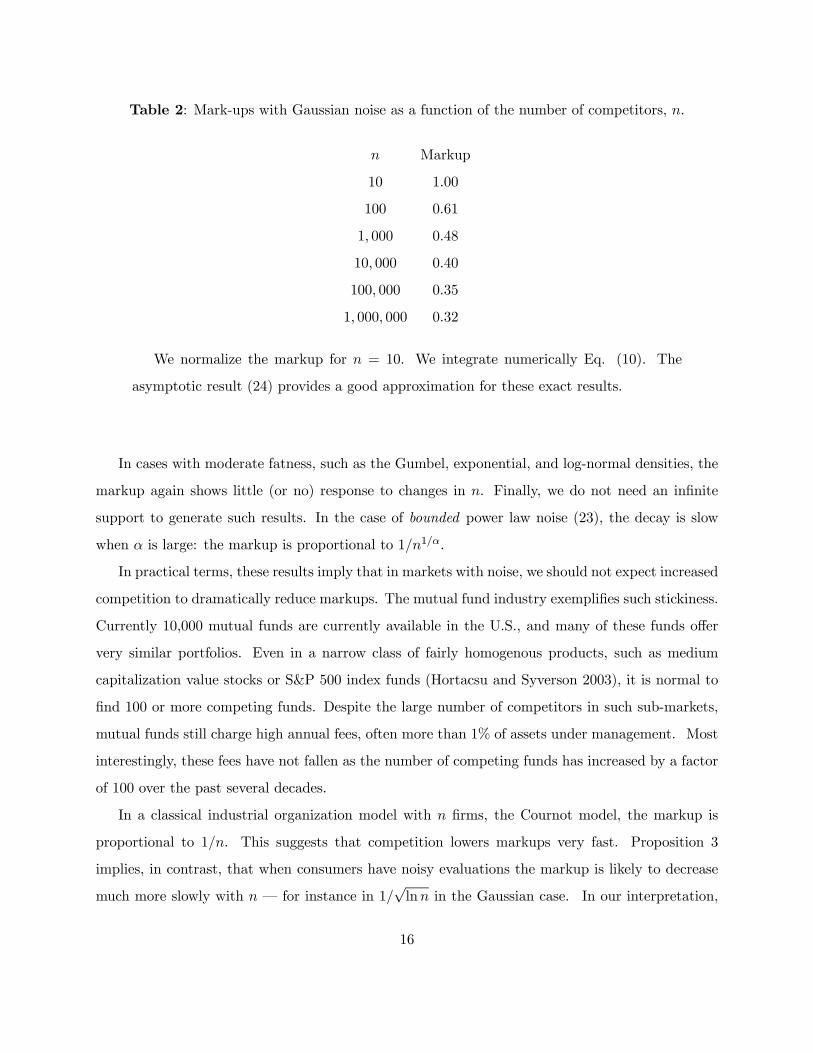
15

Table 2: Mark-ups with Gaussian noise as a function of the number of competitors, n.

n Markup

10 1.00

100 0.61

1, 000 0.48

10, 000 0.40

100, 000 0.35

1, 000, 000 0.32

We normalize the markup for n = 10. We integrate numerically Eq. (10). The

asymptotic result (24) provides a good approximation for these exact results.

In cases with moderate fatness, such as the Gumbel, exponential, and log-normal densities, the

markup again shows little (or no) response to changes in n. Finally, we do not need an infinite

support to generate such results. In the case of bounded power law noise (23), the decay is slow

when α is large: the markup is proportional to 1/n1/α.

In practical terms, these results imply that in markets with noise, we should not expect increased

competition to dramatically reduce markups. The mutual fund industry exemplifies such stickiness.

Currently 10,000 mutual funds are currently available in the U.S., and many of these funds offer

very similar portfolios. Even in a narrow class of fairly homogenous products, such as medium

capitalization value stocks or S&P 500 index funds (Hortacsu and Syverson 2003), it is normal to

find 100 or more competing funds. Despite the large number of competitors in such sub-markets,

mutual funds still charge high annual fees, often more than 1% of assets under management. Most

interestingly, these fees have not fallen as the number of competing funds has increased by a factor

of 100 over the past several decades.

In a classical industrial organization model with n firms, the Cournot model, the markup is

proportional to 1/n. This suggests that competition lowers markups very fast. Proposition 3

implies, in contrast, that when consumers have noisy evaluations the markup is likely to decrease

much more slowly with n – for instance in 1/√lnn in the Gaussian case. In our interpretation,

16

most consumers are not financially savvy and find the choice of mutual funds confusing. Noisy

evaluations make it difficult to choose among mutual funds. Because of this noise, fees remain

stubbornly high, even with 100 mutual funds in a homogeneous market. This is consistent with

equation (26), which implies that in the case of exponential noise markups do not change with

the number of firms. More generally equations (24)-(27) imply that markups will be only weakly

sensitive to the number of firms. Even when the evaluation noise is bounded, the noise can generate

a markup that decreases very slowly with n, as illustrated by the case with large α in equation

(23).

The next two subsections extend analysis of the equilibrium with exogenous noise. First we

endogenize the number of firms by considering entry (subsection 3.2) and then we consider the

impact of multiple noise sources (subsection 3.3). Readers who wish to skip these extensions can

proceed without loss of continuity to Section 4.

3.2 Extension: Endogenous Entry

We endogenize the number of firms (i.e., goods) in the industry, by assuming that firms pay a fixed

cost C of competing in an industry (in addition to marginal cost c for producing incremental units).

The marginal profit per good is p − c. Entry will endogenously determine the largest number of

firms n so that profit per firm is non-negative.

Πn =p− c

n− C ≥ 0.

Ignoring integer constraints, the free entry condition implies Πn = 0.

The following Proposition describes the impact of confusion σ and entry costs C on the number

of firms and consumer welfare. We will use the notation

bn =1

nE [f (Mn−1)], (29)

so that by Proposition 1 the markup is p− c = bnσ.

Proposition 4 Suppose that bn/n is decreasing in n, and that firms enter the market until the

zero profit condition binds. Then the number n of firms is decreasing in C/σ. Consumer welfare

17

decreases in σ. Consumer welfare increases in the entry cost C iff bn is a decreasing function.

Proof. The zero profit condition Πn = 0 implies

bn/n = C/σ, (30)

which proves that n decreases in C/σ. Consumer welfare decreases in p− c, and p− c = bnσ = nC.

So markups rise with σ (since n rises with σ) and welfare falls with σ. Finally, p − c = bnσ, so

consumer welfare decreases in C iff bn is a decreasing function.

Intuitively, as complexity, σ, increases, markups increase, consumer surplus falls, producer rents

increase, and n increases. As C increases, n falls and producer rents increase. But the effect of

C on consumer welfare depends on how bn varies with n. If b0n < 0, then markups increase and

consumer surplus falls with C. If b0n > 0, then markups will fall and consumer surplus will rise

with C. The sensitivity of the effect of C on markups and welfare is explored in Proposition 5.

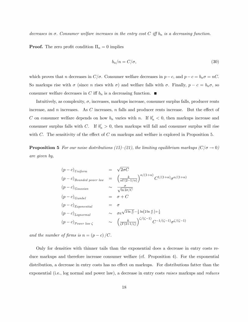
Proposition 5 For our noise distributions (15)—(21), the limiting equilibrium markups (C/σ → 0)

are given by,

(p− c)Uniform =√2σC

(p− c)Bounded power law =³

kαΓ(2−1/α)

´α/(1+α)C1/(1+α)σα/(1+α)

(p− c)Gaussian ∼ σ√ln 2σ/C

(p− c)Gumbel = σ + C

(p− c)Exponential = σ

(p− c)Lognormal ∼ σe√2 ln σ

C− 12ln(2 ln σ

C )+12

(p− c)Power law ζ ∼³

kζΓ(2+1/ζ)

´ζ/(ζ−1)C−1/(ζ−1)σζ/(ζ−1)

and the number of firms is n = (p− c) /C.

Only for densities with thinner tails than the exponential does a decrease in entry costs re-

duce markups and therefore increase consumer welfare (cf. Proposition 4). For the exponential

distribution, a decrease in entry costs has no effect on markups. For distributions fatter than the

exponential (i.e., log normal and power law), a decrease in entry costs raises markups and reduces

18

consumer welfare for the same reason that greater competition (n) raises markups in Proposition

4.

For densities at neither extreme of thin tails or fat tails (i.e. Gaussian, Gumbel, exponential,

and lognormal), welfare and markups change very little with entry costs, C. The elasticity of p− c

with respect to C is asymptotically zero for these distributions. By contrast, the number of firms,

n = (p− c) /C, is very sensitive to entry cost, with asymptotic elasticity of −1. So the bulk of ouranalysis implies that while low entry costs generate a great deal of competition, low entry costs do

not necessarily generate low markups or high consumer surplus.

3.3 Extension: Principle of Maximum Fatness

In general, we expect the noise term σε to be the sum of many components. For instance, one

might have σε = σuu+ σvv with u and v independent, mean zero, unit variance random variables.

One might guess that the equilibrium markup should depend on both σu and σv and that p − c

should be proportional topσ2u + σ2v. Appendix B shows that this is not the case. For instance,

if u and v are exponentially distributed and σu and σv are non-negative, then the markup is:

p− c = max (σu, σv). Intuitively, only the fatter-tailed noise component matters. This principle of

maximum fatness simplifies analysis.17 If there are several sources of noise, one only needs to track

the noise with the fattest tails, a point that we make more generally in Appendix B.

4 The Supply of Confusion

We return to the general case in which firms choose both the markup, p − c, and the confusion

variable, σ. For simplicity, we continue to consider the case of symmetric technologies and symmetric

equilibria. These symmetry assumptions will be in force until we relax them in subsection 4.2. We

begin by showing that firms will choose to make their products excessively complex in equilibrium.

Recall that Proposition 1 characterizes the equilibrium complexity of the good

v0 (σ) = −κn,

17This property that the fattest variable domains is the key simplifying fact in theories of extreme movements. Formore rules of that type, see Gabaix et al. (2004), Appendix A.

19

where

κn ≡ E [f (Mn−1)Mn−1]E [f (Mn−1)]

. (31)

Proposition 6 If the distribution of noise is symmetric and n > 2, then κn > 0.

Proposition 7 If κn > 0, then in the symmetric Nash equilibrium σ is strictly greater than σ∗,

the bliss point for complexity.

Proof. Since v0 (σ) = −κn, it follows that κn > 0 iff v0i (σ) < 0. Hence, σ > σ∗ since v (σ) is

hump-shaped.

To gain intuition for this result, consider a counterfactual equilibrium at which all producers

set σ = σ∗. Let firm i increase complexity. This increase in complexity has a first-order positive

effect on firm i0s market share, since more symmetric noise leads more and more consumers (at

least half of the population as σi → ∞) to buy good i.18 The increase in complexity decreases

the value v (σi) of good i, partially offsetting the gain from complexity. However, this decrease

in quality is a second-order effect local to σi = σ∗. Hence, in equilibrium firms will set σ > σ∗, so

their products are excessively complex.

4.1 Competition Increases the Supply of Confusion

We next show that competition tends to exacerbate the production of excess complexity. We work

out the analysis for three leading distributions that yield closed form expressions for κn.

Proposition 8 The equilibrium amount of complexity σ is characterized by the following expres-

sions for κn = −v0 (σ). For uniformly distributed noise (15),

κn = 1− 2n. (32)

18This is true as long as κn > 0. However, κn < 0 if the distribution of f is sufficiently skewed to the right. For thiscase, a decrease in complexity increases market share at the counterfactual equilibrium σ = σ∗. The right-skeweddistribution for ε has more mass below zero than above zero. Think about a limiting case in which all of the masslies below zero, except a small amount of mass far above zero. The mass above zero helps the producer relativelylittle, since the producer does not charge a price conditional on the realization of the noise. Hence, on net the noisehurts the producer, leading the producer to reduce the noise by opting for an inefficiently low level of complexity.Though this case is mathematically possible, we believe that it is empirically uncommon. For instance, Proposition2 shows that for all our distributions, for n high enough, κn > 0.

20

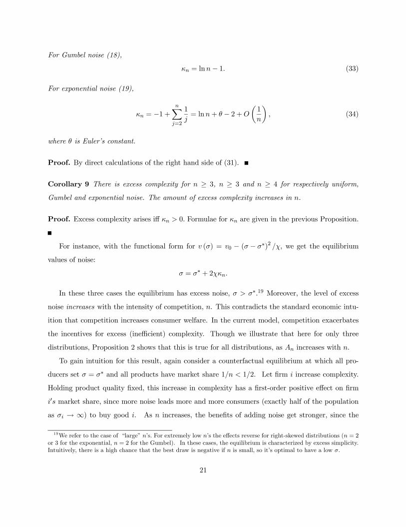
For Gumbel noise (18),

κn = lnn− 1. (33)

For exponential noise (19),

κn = −1 +nX

j=2

1

j= lnn+ θ − 2 +O

µ1

n

¶, (34)

where θ is Euler’s constant.

Proof. By direct calculations of the right hand side of (31).

Corollary 9 There is excess complexity for n ≥ 3, n ≥ 3 and n ≥ 4 for respectively uniform,

Gumbel and exponential noise. The amount of excess complexity increases in n.

Proof. Excess complexity arises iff κn > 0. Formulae for κn are given in the previous Proposition.

For instance, with the functional form for v (σ) = v0 − (σ − σ∗)2 /χ, we get the equilibrium

values of noise:

σ = σ∗ + 2χκn.

In these three cases the equilibrium has excess noise, σ > σ∗.19 Moreover, the level of excess

noise increases with the intensity of competition, n. This contradicts the standard economic intu-

ition that competition increases consumer welfare. In the current model, competition exacerbates

the incentives for excess (inefficient) complexity. Though we illustrate that here for only three

distributions, Proposition 2 shows that this is true for all distributions, as An increases with n.

To gain intuition for this result, again consider a counterfactual equilibrium at which all pro-

ducers set σ = σ∗ and all products have market share 1/n < 1/2. Let firm i increase complexity.

Holding product quality fixed, this increase in complexity has a first-order positive effect on firm

i0s market share, since more noise leads more and more consumers (exactly half of the population

as σi → ∞) to buy good i. As n increases, the benefits of adding noise get stronger, since the

19We refer to the case of “large” n’s. For extremely low n’s the effects reverse for right-skewed distributions (n = 2or 3 for the exponential, n = 2 for the Gumbel). In these cases, the equilibrium is characterized by excess simplicity.Intuitively, there is a high chance that the best draw is negative if n is small, so it’s optimal to have a low σ.

21

starting market share, 1/n, is lower. So, the incentive for higher complexity increases as n gets

large.

In summary, for the case of uniform noise, competition eliminates price inefficiencies (limn→∞ p−c = 0), but competition exacerbates the incentive for excess complexity. So the net effect on

consumer welfare is ambiguous. In the Gumbel and exponential cases, greater competition does

not eliminate pricing inefficiencies (limn→∞ p−c = σ) and competition drives complexity to infinity,

so ever greater increases in competition unambiguously reduce consumer welfare. This effect is

general for unbounded distributions. Eq. (14) shows that κn ∼ An/γ, and An →∞ for unbounded

distributions (see Table 1).

4.2 The Worst Firms Supply The Most Confusion

The discussion above showed that when firms are symmetric they will choose excess complexity of

products, σ > σ∗ where σ∗ is the socially efficient product complexity. By continuity, σ > σ∗ will

still apply, even when firms are heterogeneous, as long as the heterogeneity is minor.

In this subsection, we show that the firms with the highest extrinsic quality choose to produce

the least excess confusion. Also, we will see that when a firm is much better than the others, it

will actually choose to make its product excessively simple: σ < σ∗.

We formalize this argument with an illustrative example rather than by treating the general

case. We consider a single firm that makes endogenous decisions. It provides a good with value

v (σ) , from which consumers receive the signal v (σ) − p + σε. The value provided by exogenous

competitor firms is assumed to be a fixed number v0.20 The endogenous firm chooses σ and p to

maximize profits

π = (p− c)P (v (σ)− p+ σε > v0) . (35)

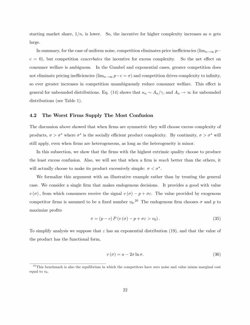
To simplify analysis we suppose that ε has an exponential distribution (19), and that the value of

the product has the functional form,

v (σ) = a− 2σ lnσ. (36)

20This benchmark is also the equilibrium in which the competitors have zero noise and value minus marginal costequal to v0.

22

Figure 1: The product’s quality v (σ) = a− 2σ lnσ as a function of its complexity σ. The value ismaximized at the “bliss” level σ∗ = e−1. The function is plotted with a = 0.

Figure 1 plots the shape of the product value function v (σ). Product value has a maximum at

σ∗ = e−1. The next Proposition describes the equilibrium choice of price p and complexity σ.

Proposition 10 When the firm maximizes profit (35) over price p and complexity σ, it sets com-

plexity equal to

σ = max³e−3/2, c+ v0 − a

´. (37)

In particular, if c+v0−a > e−3/2, then complexity decreases with the product’s quality a, increases

with the product’s production cost c, and increases with the value v0 offered by the competition. If

c+v0−a > e−1, then the firm chooses to make the product excessively complex, while if c+v0−a <e−1, the firm chooses to make the product excessively simple.

The proof is in Appendix B. Figure 2 plots the equilibrium21.

By assumption, firms have quality a and marginal cost c. If a firm has low quality or high

production costs (c + v0 − a > e−1) then it will choose excessively complex products, setting

21 In the more general case with v (σ) = a − χσ lnσ for χ > 1, the same yields σ =

max³e−1−1/χ, (c+ v0 − a) / (χ− 1)

´. As is intuitive, if the value of the product does not change much with its

complexity (χ is low), then the complexity σ∗∗ will be very sensitive to the advantages of cost or quality.

23

ExcessComplexity

Excess Simplicity

σ ∗= e-1

e-3/2

c

e-1 -v0 +a

σ

e-3/2 -v0 +a

Figure 2: This Figure plots the value of the complexity σ chosen by the firm as a function of itsmarginal cost c. See Eq. (37). Better firms (lower marginal cost) choose a lower level of complexity.There is excess complexity for c > e−1+a−v0, and excess simplicity for c < e−1+a−v0. σ∗ = e−1

is the bliss level of complexity (see Figure 1), a is the quality of the product for zero complexity,and v0 is the consumer surplus offered by the firm’ competitors.

σ = c + v0 − a > e−1 = σ∗. Intuitively, such “bad” firms generate noise with the hope that the

noise will mislead the consumers who happen to draw a noise realization in the right-hand tail.

For these consumers the noise will mask the firm’s low quality and high prices.

The better the firm, the lower the excess complexity, and the best firms choose excess simplicity

of their product. If c + v0 − a < e−1, then the equilibrium complexity will be less than σ∗. For

intuition, fix prices and consider a firm that has a particularly high quality, a >> 0. If there is no

noise in the consumers’ decisions, the superior firm will have a market share of 1. If there is some

noise, then its market share will decrease. So, a superior firm has an incentive to have very low

noise, or excess simplicity: σ < σ∗.

4.3 A Framework For Testing Endogenous Complexity

It would be easy to test these predictions about endogenous noise. For instance, Proposition 10

predicts that a mutual fund offering very low management fees would have a clear prospectus,

while funds with high fees would have an opaque prospectus. Likewise, in the cellular phone

market, plans with low prices would be simple to understand, while plans with high prices would

24

be more complicated.

The following example illustrates how such a test could be practically implemented. First,

identify mutual funds with low fees (e.g., Vanguard S&P 500 fund) and mutual funds with high fees

(e.g., Morgan Stanley S&P 500 fund). Then objectively measure the complexity of the respective

fee descriptions.

There are many sensible ways to measure complexity. For example, one could measure the

quantity of fee numbers in the fee structure. One could also count the lines of footnotes.

For example, Morgan Stanley’s S&P 500 fund prospectus contains 54 fee numbers on the 1.3

pages that summarize their fee structure. Vanguard’s S&P 500 prospectus contains 15 fee numbers

on the 0.8 pages that summarize their fee structure. Similarly, Morgan Stanley’s fee summary

contains 13 lines of footnotes, whereas Vanguard’s fee summary contains 4 lines of footnotes.22

5 The Curse of Education

So far we have assumed that firm i picks the standard deviation of noise that applies to good i (i.e.,

σi). We have shown that in most cases, firms will want to make their own products excessively

complex, σi > σ∗.

In this section, we consider another manipulation of noise. Now we assume that firm i can

educate a consumer a, and that this educated consumer will consequently have a low value of σaj

at all firms j = 1, ..., I. If consumer a is educated, the consumer will become a better judge of all

products in the marketplace.

Firms have an incentive to educate consumers – i.e., to reduce evaluation noise in the market in

general – and then to win the business of the educated consumers by offering them a low markup.

In this section, we study these incentives and show they are actually quite weak. The reasoning

is simple. After being educated, consumer a becomes a relatively low margin consumer, since

consumer a can better pick out the best deals. Hence education greatly benefits consumer a, but

only moderately benefits the firm who invests in the education. Firms that educate the public may

attract new customers, but the firms will have a small profit margin on those customers.

22Even with all of Morgan Stanley’s footnotes one still can not estimate fees without reading another seven pagesection of the prospectus that discusses “share class arrangements.”

25

The wedge between the consumer’s benefits and the firm’s benefits creates a potential ineffi-

ciency. For large education costs, the firm does not have an incentive to undertake the costly

education, even though the social benefits are positive.

Economists will naturally wonder why the consumer does not purchase education services from

a third party. In fact, we do observe such third party education. However, though the financial

education industry exists, it does not offer reliable advice. In the U.S., publications like Money

Magazine, Worth, and many others, try to market their advice every month, and hence offer a

variety of complicated strategies. Such publications have little incentive to reveal the benefits of

passive investment strategies like index funds. A person listening to such advice wouldn’t need

to hear it repeated every month. So even the financial advice industry has perverse incentives to

distort information.

We now present a formal model of the curse of education. Assume there are two types of

consumers, Sophisticates and Naives. Fraction φS of the population is sophisticated and they

have confusion parameter σS , while fraction φN is Naive, with σN À σS . Assume that the total

population of firms can be decomposed into nS firms that market to Sophisticates and nN firms

that market to Naives. In the mutual fund industry, S firms will choose to charge low fees, while N

firms will choose to charge high fees. Profits must be the same in both markets, which leads to23

π = φSbnSσS/nS = φNbnNσN/nN , (38)

where bnσ = p− c by Proposition 1 and Eq. (29).

We will say that if a firm educates a Naive consumer, it changes that consumer into a So-

phisticate for a cost K. Such education reduces the consumer’s confusion from σN to σS, and

consequently saves the consumer an amount σNbnN − σSbnS . However, the firm will be able to

make little ex-post profit on that consumer. The consumer is now a low-margin Sophisticated con-

sumer, so the firm will earn an expected profit of only σSbnN/nS on the newly educated consumer.

We summarize this conclusion with the following Proposition.

Proposition 11 A Sophisticated firm will educate a naive consumer only if the cost of education

23 Indeed, σSbnS is the profit per consumer in the S market. The total profit is thus φSσSbnS , and is divided amongthe nS firms serving this market.

26

K satisfies K < bnSσS/nS. But the consumer’s benefit from his education is bnNσN−bnSσS. Hencethere is an undersupply of education by firms when σN À σS.

6 Measuring Confusion

In principle, economists should measure the amount of confusion in the marketplace. In practice,

such measurement is difficult, because it is hard to separate intrinsic sources of demand and noise-

based motives for demand. Does an investor hold a mutual fund with a high management fee for

a good reason (e.g., he believes that the mutual fund employs great managers), or because he just

doesn’t understand the fee structure?

To cleanly measure the effects of confusion, economists should use randomized education treat-

ments (Duflo and Saez 2003, Choi et al 2004). For example, Choi et al ask subjects to allocate a

wealth windfall among a set of n mutual funds. The subjects are randomly divided into a treat-

ment group and a control group. The treatment group reads an educational background statement

before making the wealth allocation decision (e.g., “mutual funds charge management fees, which

are reported in the prospectus, etc...”). The control group makes the allocation without any educa-

tional intervention. Randomized assignment to the treatment and control groups creates two sets

of subjects who necessarily have the same ex-ante utility functions but who have different ex-post

levels of financial sophistication.

To simplify exposition, assume that the subjects in the treatment (i.e., education) group become

perfect Sophisticates as a result of the educational intervention. By contrast, the Naive subjects in

the control condition have a normal level of noise in their evaluations. Formally, the Sophisticates

– i.e., the treatment group – have no noise in their evaluations σS = 0.24 The Naives – i.e., the

control group – have σN > σS = 0.

In this example, Sophisticates and Naives have the same underlying objective function. They

differ only in their ability to maximize their preferences. Sophisticates choose optimally. Naives

would like to replicate those sophisticated choices, but end up choosing with some additional noise.

We will measure that additional noise by comparing a product’s market share of Sophisticates

to the product’s market share of Naives. When a product has a high level of confusing complexity,

24The analysis can easily be generalized to handle the case σN > σS > 0.

27

it will attract a lower share of Sophisticates than of Naives.

To formalize these ideas we will compare the demand vectors of Sophisticates and Naives:¡DSi

¢i=1...n

and¡DNi

¢i=1...n

. In the mutual fund example, DSi represents the fraction of assets

invested by the Sophisticates in mutual fund i. We will focus on a particularly important summary

statistic, ρ, the correlation between¡DSi

¢i=1...n

and¡DNi

¢i=1...n

. If there is perfect correlation

(ρ = 1) between the Sophisticates’ and Naives’ demand vectors, then there is no confusion on the

part of the Naives, implying σN = 0.25 If there is no correlation (ρ = 0), then there is full confusion

(σN = ∞). More generally, the correlation ρ between the two demand vectors allows us to infer

the precise amount of confusion.

6.1 A Tractable Econometric Framework for Measuring the Relative Impor-

tance of Confusion and True Taste Differences

We propose a tractable implementation of the above idea. We begin by assuming that a Sophisticate

has true utility USia = vi +HS (Tia) where we index consumers by a and goods by i. This utility

function depends on the idiosyncratic (true) tastes of the Sophisticate, Tia. By contrast, a Naif will

not observe her true utility, but instead only observes utility signals

UNia = vi +HN (Tia, Nia)

where Nia is noise, i.e. confusion. If the noise is always 0, i.e. Nia ≡ 0, then we will have

HS (Tia) = HN (Tia,Nia ≡ 0) . (39)

In general, the respective market shares for product i will be given by, Dτi = P

³U τia > maxj 6=i U

τja

´for τ = S,N .

We assume that idiosyncratic tastes are captured by a unidimensional source of variation,

Tia = σTuia, and that confusion noise (for Naives) is captured by a two-dimensional source of

variation Nia = (σNεia, σiηia) , where uia, εia and ηia are independent standard normals. The

25Another possible interpretation is that the education intervention was too weak to remove the confusion. In thissense, the experiment provides a lower bound on the amount of confusion σN .

28

following parametrization proves to be useful:

HN (Tia, Nia) =qσ2T + σ2NG

σTuia + σNεiaqσ2T + σ2N

+ σiηia. (40)

For reasons that will be clear soon, we choose the increasing transformation function

G (s) = − ln ln 1/Φ (s) , (41)

where Φ is the cumulative distribution function of the standard Gaussian distribution. To interpret

(40), let us start with the Sophisticates. Because of (39), their tastes shocks are HS (Tia) =

σTG (uia). We show later that G (uia) has a Gumbel distribution, which is convenient for demand

analysis. So, our model nests the basic model of product choice, which has been used so productively

in the industrial organization literature (e.g. McFadden (1981), Berry, Levinsohn and Pakes (1995),

Goldberg (1995), Nevo (2001)).

For economic and econometric generality, we allow two types of noise for the Naives: general

confusion, scaled by σN , and good-specific noise, scaled by σi. Among the naifs, we expect a high

value of σN to smooth market shares (since goods will effectively be chosen randomly), and a high

value of σi to increase the market share of good i (when n > 2). Those intuitions are formalized in

the next Proposition.

Proposition 12 With the above formulation, the demand of sophisticated consumers is

DSi =

exp¡λSvi

¢Pnj=1 exp

¡λSvj

¢ (42)

λS = 1/σT (43)

and the demand of the naives is

DNi = E

"exp

¡λNvi + λNσiηia0

¢Pnj=1 exp

¡λNvj + λNσjηja0

¢# (44)

λN = 1/qσ2T + σ2N . (45)

29

In the limit where all products have small market shares (formally, n→∞, and there is an M s.t.

for all i, var³eλ

Nvi´< M <∞), we have the following equivalence:

DNi ∼

exp¡λNvi + λNσ2i /2

¢Pnj=1 exp

³λNvj +

¡λN¢2σ2j/2

´ . (46)

If σi = 0, as λN = 1/qσ2T + σ2N is lower than λS = 1/σT , the naive’s market shares are

more dispersed. Now consider a vector of market shares within a product category (DSi ,D

Ni )

ni=1.

Consider running the following regression of the Naives’ demand on the Sophisticates’ demand:

lnDNi = α+ β lnDS

i + ri. (47)

If σi has zero (or small) covariance with vi, we will have,

β = σT /qσ2T + σ2N

Hence we expect a slope β < 1. The amount of general noise in the market is given by

σNσT

=

qβ−2 − 1.

We can also infer the amount of good-specific noise for good i

σ2i − σ2jσ2T

= 2ri

β2.

Hence the strategy for measuring confusion is quite simple: run regression (47) and impute the

value of σN/σT andσ2i−σ2jσ2T

from the resulting parameter estimates.

To implement this framework a researcher will need to identify a marketplace in which So-

phisticated and Naive agents can be distinguished ex-ante and in which the Sophisticated and

Naive agents have the same underlying distributions of objective functions. These are not trivial

requirements, but they can be surmounted with randomized field experiments: randomly select

a subpopulation of consumers, educate them about an industry (e.g., mutual funds), and then

compare their demand vectors to a control group.

30

6.2 Measuring the Distribution of the Noise

Until now, the analysis in this section has assumed a particular functional form for the distribution

of noise. This subsection shows how to estimate the distribution when the functional form is

unknown.

Suppose that a decision-maker evaluates a set of n goods (e.g., mutual funds). The decision-

maker then ranks his two favorite goods and reports the price difference, ∆pn, that makes him

indifferent between them.26 It turns out that the relationship between ∆pn and n, the number of

goods, can be used to impute the shape of the noise distribution.27 To see how this works, first

observe that ∆p = σ¡ε(1) − ε(2)

¢, where ε(1) and ε(2) are the highest and second highest draws of

n i.i.d. signals. We will want to exploit the following Proposition.

Proposition 13 The expected value of ∆pn is:

∆pn ∼ bnΓ (2 + ξ)Γ (1− ξ) (48)

where bn =p−cσ , and p−c is calculated in Proposition 10. In particular, for the Gaussian, Gumbel,

exponential, and log-normal distributions ∆pn ∼ bn.

The proposition implies that∆pn is a good approximation of bn, up to a constant, Γ (2 + ξ)Γ (1− ξ),

which does not depend on n and which will be approximately equal to one in the Gaussian, Gumbel,

exponential and lognormal cases.

We now have all of the results that we need to infer the underlying noise distribution. The

imputation relies on the following data: measures of the gap ∆pn for a variety of market sizes n,

for instance n = 10, 50 and 200. To impute the distribution of noise, graph ln∆pn as a function

lnn. Its slope should be the characteristic index ξ of the distribution.

26We assume that all preferences are measured with incentive compatible mechanisms.27We have exact results in two cases. For the uniform distribution, ∆pn = 2σ/ (n+ 1), and the the exponential

distibution ∆pn = σ. The derivations are by simple calculations from e.g. Reiss (1989, Chapter 1).

31

7 Conclusion

We have analyzed an environment in which consumers have noisy evaluations of products. The

noise effectively increases the market power of firms, raising equilibrium markups. Competition

barely reduces this market power. If consumers have noisy product evaluations, high levels of

competition have little effect on markups.

We also analyze markets in which firms can influence the level of noise, or product complexity.

In equilibrium, firms choose to make products excessively complex (i.e., excessively noisy) and com-

petition only exacerbates this problem. Higher levels of competition increase the equilibrium level

of excess complexity. Here again, competition does not protect consumers from the consequences

of noisy evaluations. We also show that firms with the highest unit costs and the lowest product

quality will choose the greatest excess complexity.

We present an econometric framework that measures confusion in the marketplace. Randomly

divide a population of consumers into two groups: control and treatment. Observe the control

group’s market purchases (e.g., mutual fund selection). Educate the treatment group and then

observe their market purchases (e.g., teach the treatment group how to read a mutual fund prospec-

tus and then observe their mutual fund selection). If the control group chooses differently than

the treatment group, then the choices of the control group are driven partially by confusion. We

show how to use market demand vectors to econometrically impute the quantity of noise in the

marketplace.

32

8 Appendix A: Elements of Extreme Value Theory

Coefficients of Regular Variation We recommend Embrechts et al. (1997) and Resnick

(1987) for excellent expositions of extreme value theory. The following concept will be important

in the proofs.

Definition 14 A function g defined in a right neighborhood of 0 has regular variation with exponent

ρ if

∀u > 0, limt→0+

g (ut) /g (t) = uρ. (49)

This means that, for small t > 0, g (t) behaves like tρ, perhaps up to a constant or slowly

varying function. For instance, (49) holds if g (t) = tρ and g (t) = tρ [ln (1/t)]α for some α. If the

following limit exists, it provides a convenient characterization of ρ (see Resnick 1987, p.21):

ρ = limt→0+

tg0 (t)g (t)

. (50)

Three Types of Distributions In extreme value theory, there are three classes of distribu-

tions. They are ordered by increased fatness of the right tail. A useful indicator of their fatness is

a the characteristic index ξ. ξ is the coefficient of regular variation28 of f³F−1(t)´/t for t → 0.

There are alternative, similar, definitions (Embrechts et al. 1997, p.152-158). As Table 1 indicates,

ξ is an index of the fatness of the distribution. Distributions with fatter tails have a (weakly) larger

ξ.

The first type is the “domain of attraction of the Weibull”. It comprises very “thin tailed”

distributions of the type (16), such as the uniform distribution. Their support has an upper bound.

For them ξ = −1/α.The second type is the “domain of attraction of the Gumbel”. It comprises distributions of

medium thinness, such as the Gaussian, Gumbel, Exponential, and Gamma distributions. Their

support is unbounded on the right, and ξ = 0.

The third type is the “domain of attraction of the Fréchet.” It comprises power law tail distri-

butions of the type (21). Here ξ = 1/ζ.

28So ξ ≡ −1 + limt→0+ t ddtlnhf³F−1(t)´i.

33

9 Appendix B: Longer Derivations

9.1 Two Basic Propositions

The following result will characterize the large n behavior of E [J (Mn−1)], where J is a function,

andMn−1 = maxi=1...n−1 εi is the maximum of n−1 random variables with CDF F . Define F (x) ≡1−F (x). The following Proposition allows us to replace the complicated integral E [J (Mn−1)] by

the simpler deterministic expression J (An)Γ (1 + ρ).

Proposition 15 Consider a function J such that J³F−1(t)´has coefficient of regular variation

ρ, and Mn−1 is the maximum of n− 1 i.i.d. random variables with CDF F . Set (An) = F−1(1/n).

Then:

limn→∞

E [J (Mn−1)]J (An)Γ (1 + ρ)

= 1 (51)

Proof. We call mn−1 = mini=1...n−1 yi the minimum of n− 1 i.i.d. uniform [0, 1] variables yi. Its

cumulative is:

P (mn−1 > t) = P (∀i = 1...n− 1, yi > t) =n−1Yi=1

P (yi > t) = (1− t)n−1 (52)

Mn−1 has the distribution: P (Mn−1 < X) = F (x)n−1. So Mn−1 has the same distribution as

F−1(mn−1). Indeed:

P³F−1(mn−1) < X

´= P

¡mn−1 > F (x)

¢=¡1− F (x)

¢n−1by (52)

= F (x)n−1 = P (Mn−1 < X) .

Defining j (t) = J³F−1(t)´, this yields the representation

In ≡ E [J (Mn−1)] = EhJ³F−1(mn−1)

´i= E [j (mn−1)] .

Before proceeding, we give some intuition for why the result should be true. Given that mn−1

is concentrated around its mean, 1/n, the last equation makes plausible that In ' j (1/n). This

reasoning gives the leading order term for In. Taking into consideration the fluctuations of mn

34

around its mean, we get a subleading correction.

In = E [j (mn−1)] =Z 1

0j (x) (n− 1) (1− x)n−2 dx

=

Z n

0j³un

´ n− 1n

³1− u

n

´n−2du.

As¡1− u

n

¢n−1 → e−u, we have

In ∼Z n

0j³un

´e−udu = j

µ1

n

¶Z n

0

j (u/n)

j (1/n)e−udu

∼ j

µ1

n

¶Z n

0uρe−udu ∼ j

µ1

n

¶Z ∞

0uρe−udu = j

µ1

n

¶Γ (1 + ρ) .

The assumption of unbounded support is not crucial. What matters here is the behavior of

the density around An. So the above results hold if the distribution of the noise is truncated

on the right by some X, if F (X) ¿ 1/n. One replaces the index ρ by its local equivalent,

ρ = j0 (1/n) / [nj (1/n)]. Numerical simulations show that this gives very good results.

Characterizing the Exponents The following two Propositions will be useful.

Proposition 16 For a regular distribution with characteristic index ξ, the coefficient of regular

variation of f³F−1(t)´is 1 + ξ.

Proposition 17 For a regular distribution with characteristic index ξ, if the upper bound of F ’s

support is∞ or a non-zero real number, then the coefficient of regular variation of f³F−1(t)´F−1(t)

is 1 +min (0, ξ).

The proofs are typically easy for power law distributions, which have ξ 6= 0. The results for

ξ = 0 can be guessed by continuity, but require slightly more careful arguments.

Proof of Proposition 16. To reduce the algebraic clutter, in the derivations we omit the

corrections due to the “slowly varying functions”, and set the scaling constants k at 1. If F is in

the domain of attraction of the Fréchet (as in Eq. 21), write f (x) = ζx−ζ−1, and F = x−ζ . Then

F−1(t) = t−1/ζ , and f

³F−1´

(t) = ζt1+1/ζ . Because in this case ξ = 1/ζ, this means ρ = 1 + ξ.

35

If F is in the domain of attraction of the Weibull (as in Eq. 16), the same proof works.

We say that the upper bound is 1, and have f (x) = α (1− x)α−1, and F = (1− x)α. Then

F−1(t) = 1 − t1/α, and f

³F−1´

(t) = αt1−1/α. Because in this case ξ = −1/a, this meansρ = 1 + ξ. If F is in the domain of attraction of the Gumbel, Resnick (1987, p. 66) shows:

t ddt lnhf³F−1(t)´i= −F (x) f 0 (x) /f (x)2 → 1, which implies ρ = 1. ¤

Proof of Proposition 17. We call ρg the coefficient of regular variations of a function g.

If ξ > 0 and F−1(t) = t−1/ζ = t−ξ, then ρ

F−1 = −ξ. See Resnick (1987, pp. 63-67), along with

the case ξ = 0. For ξ < 0, F−1(t) converges to a non-zero upper bound of the distribution, so

ρF−1(t)= 0. We conclude that ρ

F−1(t)= min (−ξ, 0). To finish the proof, we observe that, for two

functions g and h, (49) implies ρg·h = ρg + ρh. We apply this to find

ρf³F−1(t)´F−1(t)

= ρf³F−1(t)´ + ρ

F−1(t)

= 1 + ξ +min (−ξ, 0) = 1 +min (0, ξ) . ¤

9.2 Proof of Proposition 1

The firm’s maximization problem is given by maxxi,σi (pi(xi, σi)− c)D (xi, σi). Using (4), the

associated first order conditions are

−D (xi, σi) + (pi − c)∂

∂xiD (xi, σi) = 0,

v0i (σi)D (xi, σi) + (pi − c)∂

∂σiD (xi, σi) = 0.

At a symmetric equilibrium (pi = p, xi = 0, σi = σ), substitution of equations (7), (8), and (9)

yields

− 1n+ (p− c)

1

σE [f (Mn−1)] = 0,

v0 (σ)1

n+ (p− c)

1

σE [f (Mn−1)Mn−1] = 0,

which can be rearranged to produce the required results.

36

9.3 Proof of Proposition 2

For p− c, Proposition 16 says that the coefficient of regular variations of f³F−1(t)´is ρ = 1+ ξ.

So applying Proposition 15 to J (x) = f (x) gives: E [f (Mn−1)] ∼ f (An)Γ (2 + ξ). Substituting

this into (10) we get (13).

For v0 (σ), Proposition 17 says that the coefficient of regular variations of f³F−1(t)´F−1(t)

is ρ = 1 + min (0, ξ). Proposition 15 applied to J (x) = f (x)x gives: E [f (Mn−1)Mn−1] ∼f (An)AnΓ (2 + min (0, ξ)). Eq. (11) gives:

−v0 (σ) = E [f (Mn−1)Mn−1]E [f (Mn−1)]

∼ f (An)AnΓ (2 + min (0, ξ))

f (An)Γ (2 + ξ)=

An

Γ (2 + max (0, ξ)).

9.4 Proof of Proposition 5

The markup is p − c = bnσ = (bnσ/n)n = Cn and n solves (30). By homogeneity, it is enough

to consider the case C = 1 and the limit σ → ∞. In the case where n cannot be solved exactly,we use the method of iterated approximations.29 This calculation is straightforward, except in the

Gaussian and lognormal cases. In the Gaussian case, we have bn/n ∼ 1/hn√ln 2n

i∼ 1/σ, so

lnn = lnσ − 12ln (ln 2n) + o (1) = lnσ − 1

2ln

µln 2 + lnσ − 1

2ln (ln 2n)

¶+ o (1)

= lnσ − 12ln (ln 2σ + o (lnσ)) + o (1)

= lnσ − 12ln (ln 2σ) +

1

ln 2σo (lnσ) + o (1) by Taylor expansion

= lnσ − 12ln (ln 2σ) + o (1)

which proves the result for (p− c)Gaussian. The lognormal case is similar.

29See e.g. Resnick (1987, p.67-74).

37

9.5 Proof of Proposition 6

The denominator of (31) is positive, and the numerator isE [f (Mn−1)Mn−1] =R(n− 1)xf (x)2 F (x)n−1 dx.

If f is symmetric around 0, then

E [f (Mn−1)Mn−1] =Zx>0

(n− 1)xf (x)2hF (x)n−1 − F (−x)n−1

idx > 0.

9.6 Proof of Proposition 10

By shifting a into a0 = a− c− v0 and p into p0 = p− c we can assume c = v0 = 0 in the proof. We

are looking for the optimal complexity level, which we will call bσ in this proof. The profit functionis:

π = pP (v (σ)− p+ σε > 0) = pP

µε >

p− v (σ)

σ

¶= pmax

³e−

p−v(σ)σ

−1, 1´.

We consider first the case where we have an interior solution ,

e−p−v(σ)

σ−1 < 1. (53)

Then the price p that maximizes the profit π is p = σ, and the profit is π = σev(σ)/σ−2. Using

the function form (36) we get: lnπ = aσ − lnσ − 2. If a ≥ 0, the maximum is at σ = 0, which

violates (53). If a < 0, the maximum is at bσ = −a. Condition (53) holds iff0 > −bσ − v (bσ)bσ − 1 = v (bσ)bσ − 2 = abσ − 2 ln bσ − 2 = −2 ln bσ − 3,

i.e. −a = bσ > e−3/2.

If this last condition does not hold, then (53) binds, and π = p = v (σ) − σ, and whose

maximization gives σ = argmaxσ v (σ)− σ = e−3/2. This proves (37).

9.7 Proof of Proposition 12

First we observe that for s a standard normal, G (s) has a Gumbel distribution,

P (G (s) < x) = P¡s < G−1 (x)

¢= Φ

¡G−1 (x)

¢= e−e

−x.

38

So GµσTuia+σNεia√

σ2T+σ2N

¶is a Gumbel variable, and we have, by the standard result on logit demands30,

Di = DNi = E

"exp

¡λNvi + λNviηia0

¢Pnj=1 exp

¡λNvj + λNvjηja0

¢ | (vj)1≤j≤n#

(54)

with λN as in (45). Replacing σn and vi in the above formula yields the formula (42) for the

sophisticates.

The derivation of asymptotic formula (46) is straightforward.

9.8 Proof of Proposition 13

We use the results in Reiss (1989, p.161), and direct calculations. For instance, in the unbounded

power law case with k = 1, the asymptotic CDFs of n−1/ζε(1) and n−1/ζε(2) are F(1) = e−x−ζ and

F(2) = e−x−ζ¡1 + x−ζ

¢, so:

n−1/ζ∆pn = Ehn−1/ζε(1) − n−1/ζε(2)

i→Z ∞

0x³F 0(1) − F 0(2)

´dx

=£x¡F(1) − F(2)

¢¤∞0−Z ∞

0

¡F(1) − F(2)

¢dx =

Z ∞

0e−x

−ζx−ζdx =

1

ζΓ

µ1− 1

ζ

¶

The calculation is similar for the other types of distributions.

9.9 Existence of a Symmetric Equilibrium

This section discusses conditions under which a symmetric equilibrium exists. By shifting all the

variables by −c, it is sufficient to study the case c = 0. By homogeneity, it is sufficient to study

the case σ = 1. We define D (x) = D (x, σ = 1).

By Proposition 1, a symmetric equilibrium can only exist at p = bn. A global symmetric

equilibrium exists iff the profit function pD (bn − p) has a global maximum for p = bn. A local

equilibrium exists iff the profit function pD (bn − p) has a local maximum at p = bn. We next

review what is known about the existence of equilibrium in such cases.

It can be shown that p = bn is a global equilibrium if ln f is concave. However, this sufficient

condition is not necessary. A global equilibrium also exists in other natural cases, e.g., for the

30See e.g. Anderson et al. (1992), p. 39.

39

log-normal distribution. We can prove the existence of a local equilibrium in the log-normal case,

and can verify that the equilibrium is global using numerical methods. Complete analytic proofs of

the existence of a symmetric equilibrium for non-log concave distributions (such as the lognormal

distribution) is an open problem in mathematical economics (cf. Caplin and Nalebuff 1991).

While it would be useful to have analytic results for the global equilibrium, for many purposes

this is not necessary. For a given distribution and value of n, the check can be done numerically.

Hence as a check for our Proposition that the markup increases in n for a lognormal distribution,

one can check that, for n = 2...100, that p − c = bn is indeed a global equilibrium. This confirms

our statement that the markup increases in n for lognormal distributions, as least for n = 2...100.

We now detail our arguments. First, we recall standard conditions for the existence and unique-

ness of an equilibrium.

Proposition 18 If ln f is concave, an equilibrium exists and is unique.

Proof. We apply Caplin and Nalebuff (1991), Theorem 2 and Proposition 7.

The above proposition is useful for distributions less fat than the exponential (such as the

distributions (15)— (19)). But the proposition is not powerful enough for fatter distributions, such

as the lognormal. We verified numerically that the equilibrium exists for distributions (20)- (21),

which have finite variance. Also, we can derive the following mathematical criterion to show that

the equilibrium is at least local, i.e. that pD (bn − p) has a local maximum at p = bn. We then

derive its limit behavior.

Proposition 19 The profit function π (p) = pD (bn − p) satisfies π0 (bn) = 0, and we have π00 (bn) <

0, i.e. a strict local maximum, iff ρn < 2, where the normalized curvature ρn is:

ρn ≡−E [f 0 (Mn−1)]nE [f (Mn−1)]2

. (55)

Proof. Profit πi (pi) = piD (bn − pi). At p = bn, we have p = 1/ (nD0) and π00 (bn) = pD00 − 2D0,

implying that π00 (bn) < 0 iff D00nD0 − 2D0 < 0, i.e., ρn = D00

i

£nD02

i

¤−1< 2. We conclude using

D00 (0) = E [−f 0 (Mn−1)] and D0 (0) = E [f (Mn−1)].

Proposition 20 We have

limn→∞ ρn = ρ∞ =

Γ (2 + 2ξ)

Γ (1 + ξ)Γ (2 + ξ), (56)

40

ρ∞< 2, for all the distributions in Table 1 (including power law distributions provided they have

finite variance).

Proof. Define h (t) = −f 0³F−1(t)´. Proposition 15 implies ρn ∼ ρ (1/n) where

ρ (t) ≡ th (t)Γ¡1 + ρh

¢h (t)2 Γ (2 + ξ)2

.

First, we consider the case ξ = 0. Embrechts et al. (1997, p.140) show that as x → ∞,−f 0 (x) /f (x) ∼ f (x) /F (x). This implies that for t → 0, h (t) ∼ h (t)2 /t. So ρh = 1 and

ρ (t) = th(t)2/t

h(t)2∼ 1. Hence limn→∞ ρn = 1, and the Proposition is verified as ξ = 0.

Next, we consider ξ > 0. (The proof is the same if ξ < 0.) For F (x) ∼ kζx−ζ , F−1 (t) ∼ kt−1/ζ ,

and

h (t) = f³F−1(t)´∼ ζ

kt1+1/ζ

h (t) = −f 0³F−1(t)´∼ ζ (ζ + 1)

k2t1+2/ζ ,

so that ρh = 1 + 1/ζ, ρh = 1 + 2/ζ = 2ρh − 1 and

ρ (t) =th (t)Γ

¡1 + ρh

¢h (t)2 Γ (1 + ρh)

2 ∼ζ(ζ+1)k2

t2+2/ζΓ (2ρh)³ζk t1+1/ζ

´2Γ (1 + ρh)

2=

Γ (2 + 2ξ)

Γ (1 + ξ)Γ (2 + ξ).

For instance, for the Gaussian, exponential and lognormal distributions (which have βh = 1),

ρ∞ = 1, which implies that for large n the equilibrium is indeed locally stable.

Also, for power law distributions with exponent ζ (Eq. 21), for large n, the equilibrium is locally

stable if ζ ≥ 2, which implies ρn < 2. Extensive numerical work leads us to conjecture that it is

globally stable, but we could not prove this formally. Interestingly, the equilibrium is not globally

stable for the power laws that have ζ < 2 , i.e. that have infinite variance.

In summary, using analytic and numerical results we have shown that the symmetric equilibrium

exists for our distributions with finite variance, but a completely analytic proof is beyond the scope

of this paper. We offer a simple numerical way to check that p = bn is a global equilibrium, so

41

that in any particular application one can check that our assumption of a symmetric equilibrium

is verified.

9.10 The Maximum Fatness Principle

In general, we expect the noise term σεi to be the sum of several influences. For instance, one can

have σε = σuu + σvv with u and v independent. One might expect that the markup will depend

on both noise intensities, implying that p− c would be proportional to σu + σv for instance. The

following Proposition shows that this is not the case.

Proposition 21 If u and v are exponentially distributed with mean 0 and variance 1 and the total

noise is σε = σuu+ σvv, then the markup is p− c = max (|σu| , |σv|) .

Proof. By homogeneity it is enough to consider the case σu = 1 > σv > 0. The density of u and

v is e−x−11x>−1, hence the tail distribution of σuu+ σbv is:

G (x) = P (u+ σvv > x) =

Z Zu>−1,v>−1

e−u−v−21u+σbv>xdudv

=e−σv−1

1− σve−x +

σve−/σv−1

1− σve−x/σv ∼ e−σv−1

1− σve−x

hence G (x) is tail equivalent (Resnick 1987, p.67) to an exponential distribution. We use Proposi-

tion 2 to conclude.

Intuitively, the fatter tail dominates the sum. This is likely to be quite general. We conjecture

that if u has fatter tails than v, in the sense that limt→∞£Fu (t) /fu (t)

¤/£F v (t) /fv (t)

¤=∞ then

σuu+ σbv is tail-equivalent to σuu, and the equilibrium markup is the markup that would occur if

the noise were only σuu.

10 Appendix C. Variety of Bayesian Inferences

We consider the case where consumer a has a true utility for good i, Via = vi − pi + σTuia, but

receives a noisy signal,

Uia = vi − pi + σTuia + σNεia.

42

Here σTuia is true variation in tastes and σNεia is just evaluation noise. In the body of the paper,

we assume that consumer choose the good with the largest Uia, because we view this an a useful

benchmark. This section discusses the choices of a Bayesian consumer31. We first explore cases in

which all the vi and σN are equal.

10.1 Case Where Just One Signal is Observed

Suppose the consumer observes just Uia but not pi (for instance, the price itself is unclear, as in a

checking account or a mutual fund, or the quality to price ratio itself is unclear). The consumer

should rationally choose the good i that maximizes E [Via | Uia]. Under weak conditions32, this is

equivalent to maximizing Uia.

10.2 Case Where Just a Quality Signal and a Price Signal are Observed

We take the case of Gaussian noise. E [Via | Uia, pi] = vi − pi + λ (σTuia + σNεia), where λ is the

traditional signal-extraction factor: λ = 1/³1 + σ2e,N/σ

2e,T

´with σ2e,N/σ

2e,T the ratio of noise to

true differentiation, as perceived by the customer. The decision utilities are therefore:

E [Via | Uia, pi] = vi − pi + νwia (57)

ν = λqσ2T + σ2N (58)

and wia is a standard normal. The treatment of the paper follows, with the effective noise ν.

For instance, one has, in the Bertrand case: p − c = bnν where bn is the value calculated for the

Gaussian noise.

10.2.1 Case of Market-Unspecific Expectations

If consumers do not have a theory of the market specific noise, they will use a signal-extraction λ

that is independent of σ2N/σ2T . Then, we have p− c = bnλ

qσ2T + σ2N . So that again, the markup

31Anantham and Ben-Shoham (2004) examine the strategy of a monopolist with Bayesian consumers.32We thank Avinash Dixit for providing us with a simple sufficient condition. It is that the distribution of Via

should undergo a first-order stochastic dominant shift to the right as Uia increases. So if F (Via | Uia) is the cumulativedistribution function of Via given Uia, the condition is ∂F (Via | Uia) /∂Uia ≤ 0. Here all firms have the same amountof noise σ.

43

will increase as a function of the noise σN , and the conclusions of our analysis go through.

10.2.2 Case of Market-Specific Expectations

An example where confusion decreases profits under rational expectations In this case

σ2e,N/σ2e,T = σN/σ

2T . Then, (57) gives

ν = σ2T/qσ2T + σ2N . (59)

Thus, when the noise σN increases, the markup decreases. To understand this effect and assess its

robustness, consider the case where σT = 0, σN > 0. There is no true heterogeneity in quality, so

consumers should just use the rule “pick the lowest price, irrespective of quality,” and the markup

is 0, as in (59). This is not, however, a stable equilibrium once we allow for entry with arbitrary

qualities. Firms would take advantage of this rule to enter with very low quality products, and so

the rule “pick the lowest price” would not be valid any more. Consumers would have also to pay

attention to the perceived quality of the product. Here the consumer noise σN would determine

the dispersion in the quality of the product. We will not present a general analysis of the case with

heterogenous qualities. Instead, we present an example where confusion increases profits.

An example where confusion increases profits under rational expectations There are

three firms indexed by i = 1, 2, 3. The qualities are q1 = q2 = 6, q3 = 0, and the unit costs are

c1 = c2 = 2, c3 = 1. The consumer will buy at most one good. He has utility qe − p if he buys one

good with expected value qe and price p, and 0 otherwise. Firm i can post a price pi ≥ 0, or exitthe market.

If there is no confusion, then in equilibrium p1 = p2 = 2 and firm 3 can post any positive price

but does not sell anything.33 We have a Bertrand equilibrium where the aggregate profit is

πNo Confusion =3X

i=1

πi = 0. (60)

For simplicity, to study the effects of confusion we now consider the case of infinite confusion.

33We could postulate that firm 3 has to pay a small positive price to stay in the market. Then, there is uniqueequilibrium where firm 3 exits the market, firms 1 and 2 stay in the market, and p1 = p2 = 2.

44

We assume that consumers cannot evaluate qualities at all, though they can see prices. We assume

rational expectations. The equilibrium decision rule picks a product randomly from the set of goods

with the lowest price. Call the equilibrium price p. We shall see that p = 2. Indeed, if p > 2, there

is an incentive for firm 1 or 2 to charge a slightly lower price p0 = p− δ, δ > 0 small; it would get

the whole market and thus see a discrete increase its profit from (p− 2) /3 to (p− 2− δ). So, we

cannot have p > 2.

If p < 2 firms 1 and 2 make negative profits (p − 2)/3 if they are still in the market. So themarket is just composed of firm 3, and the rational expectation on the quality is qe = 0. To get

non-negative surplus qe−p, we need p = 0, but then firm 3 makes losses as c3 > 0, and thus shouldexit the market. So p < 2 is not possible either. We conclude that the equilibrium is characterized

by p = 2. The rational expectation of the quality is qe =³P3

i=1 vi

´/3 = 4, which yields a positive

surplus for the consumer. It is easy to see that no firm has an incentive to deviate. Each firm has

1/3 of the market, and the aggregate profits are:

πFull Confusion =3X

i=1

πi =3X

i=1

1

3(p− ci) =

1

3. (61)

The aggregate profit under full confusion, (61), is higher than the profit under no confusion

(60). The economic origin of this is that the low quality firm takes advantage of the confusion

to get some market share and obtain positive profits. The two high quality firms still are at a

Bertrand, zero-profit state (p = c1 = c2 = 2), as in the situation with no confusion.

We conclude that the phenomenon of confusion-induced increases in profits is consistent with

rational expectations in at least some cases. In our second example confusion decreases profits. It

would be useful to have a complete characterization of rational expectation equilibria with confu-

sion. The general analysis would be rather involved, including analysis of non-symmetric Bayesian

equilibria and some conceptually problematic equilibrium selection issues. Such a characterization

is a mathematically challenging topic for further research.

45

11 References

Alexander, Gordon, Jonathan D. Jones, and Peter J. Nigro (1998). “Mutual Fund Shareholders:

Characteristics, Investor Knowledge, and Sources of Information.” Financial Services Review,

7, 301-16.

Anantham, Siva and Assaf Ben-Shoham (2004) “Quality Uncertainty and Monopolistic Pricing,”

Harvard Mimeo.

Anderson, Simon, André de Palma and Jacques-Francois Thisse, Discrete Choice Theory of Prod-

uct Differentiation, MIT Press, 1992.

Anderson, Simon, Jacob Goeree and Charles Holt, “Rent Seeking with Bounded Rationality: An

Analysis of the All-Pay Auction,” Journal of Political Economy (1998), 828-853.

Barber, Brad M., Terrance Odean, and Lu Zheng (2002). “Out of sight, out of mind: The effects

of expenses on mutual fund flows.” Mimeo, U.C. Davis.

Bénabou, Roland, and Robert Gertner “Search with Learning from Prices: Does Increased In-

flationary Uncertainty Lead to Higher Markups?,” Review of Economic Studies, 60 (1993)

69-95.

Benartzi, Shlomo, and Richard Thaler, “Naive Diversification Strategies in Retirement Saving

Plans,” American Economic Review 91 (2001) 79-98.

Benartzi, Shlomo, and Richard Thaler, “How Much Is Investor Autonomy Worth?” Journal of

Finance 57 (2002), pp. 1593-1616.

Bertrand, Marianne, Dean Karlan, Sendhil Mullainathan, Eldar Shafir and Jon Zinman (2004)

“Pricing Psychology: A Field Experiment”. Mimeo.

Caplin, A., and B. Nalebuff, “Aggregation and Imperfect Competition,” Econometrica, 1991, 25-

60.

Choi, James, Xavier Gabaix, David Laibson, and Brigitte Madrian (2004). “Measuring Noise.”

Harvard mimeo.

46

Cronqvist, Henrik and Richard H. Thaler (2004) “Design Choices in Privatized Social Security

Systems: Learning from the Swedish Experience,” American Economic Review (Papers and

Proceedings).

DellaVigna, Stefano, and Ulrike Malmendier (2002) “Overestimating Self-Control: Evidence from

the Health Club Industry,” mimeo.

De Palma, André, Gordon M. Myers, and Yorgos Y. Papageorgiou, “Rational Choice Under an

Imperfect Ability To Choose,” The American Economic Review, Vol. 84, No. 3. (Jun., 1994),

pp. 419-440.

Diamond, Peter, “A Model of Price Adjustment,” Journal of Economic Theory, 1971, 156-68.

Duflo, Esther and Emmanuel Saez, “The Role of Information and Social Interactions in Retirement

Plan Decisions: Evidence from a Randomized Experiment,” Quarterly Journal of Economics,

Vol. 118 (3), 2003.

Ellison, Glenn and Drew Fudenberg, “Rules of Thumb for Social Learning,” Journal of Political

Economy 101 (1993), 612-643.

Embrechts, P., Kluppelberg, C., and Mikosch, T. Modelling Extremal Events (Springer Verlag,

New York, 1997).

Gabaix, Xavier, Parameswaran Gopikrishnan, Vasiliki Plerou, H. Eugene Stanley “A Theory of

Power Law Distributions in Financial Market Fluctuations,” Nature, 423 (2003), 267—30.

Gabaix, Xavier, David Laibson (2004) “Shrouded Attributes and Information Suppression in Com-

petitive Markets,” Harvard and MIT Manuscript.

Glaeser, Edward (2003) “The Political Economy of Hatred,” Harvard mimeo.

Goldberg, Pinelopi. “Product Differentiation and Oligopoly in International Markets: The Case

of the U.S. Automobile Industry,” Econometrica, July 1995, pp. 891-951.

Hall, Robert (1997) “The Inkjet Aftermarket: An Economic Analysis,” Stanford mimeo.

47

Heidhues, Paul and Botond Koszegi. “Loss Aversion, Price Stability, and Sales”. Berkeley manu-

script (2004).

Hortacsu, Ali and Chad Syverson (2004) “Product Differentiation, Search Costs and Competition

in the Mutual Fund Industry: A Case Study of S&P 500 Index Funds,” Quarterly Journal of

Economics.

Investment Company Institute, Mutual fund fact book, 43rd edition (2003).

Judd, Kenneth and Mike Riordan (1994), “Price and Quality in a New Product Monopoly,” Review

of Economic Studies, 61, 773-789.

Kahneman, Daniel, and Amos Tversky, “Prospect Theory: An Analysis of Decision under Risk”,

Econometrica 47 (1979), 263-291.

Koszegi, Botond and Rabin, Matthew (2003) “Modeling Reference-Dependent Preferences,” Berke-

ley mimeo.

Luce, R. D., Individual Choice Behavior, New York: John Wiley, 1959.

Madrian, Brigitte C. and Dennis F. Shea (2001), “The Power of Suggestion: Inertia in 401(k)

Participation and Savings Behavior,” Quarterly Journal of Economics, 116(4), p.1149-1187.

McFadden, D. “Econometric models of probabilistic choice.” in C. Manski and D. McFadden, eds.,

Structural analysis of discrete data, pp. 198-272, Cambridge, MIT Press, 1981.

Mullainathan, Sendhil and Andrei Shleifer (2003) “The Market for News”. NBER WP.

Nevo, Aviv. “Measuring Market Power in the Ready-to-Eat Cereal Industry,” Econometrica,

69(2), 307-342, 2001.

Oster, Sharon M. and Fiona M. Scott Morton (2004) “Behavioral Decision-Making: An Applica-

tion to the Setting of Magazine Subscription Prices”. Yale mimeo.

Perloff, Jeffrey M. and Steven C. Salop. “Equilibrium with Product Differentiation,” The Review

of Economic Studies, Vol. 52, No. 1. (Jan., 1985), pp. 107-120.

48

Reiss, R., Approximate Distributions of Order Statistics, (Berlin, Germany: Springer Verlag, 1989).

Resnick, Sidney. Extreme Values, Regular Variation, and Point Processes. Springer Verlag, 1987.

Rosenthal, Robert “A Model in which an Increase in the Number of Sellers Leads to a Higher

Price,” Econometrica, 48(6), p.1575-9, 1980.

Salop, Steven and Stliglitz, Joseph “Bargains and Ripoffs: A Model of Monopolistically Compet-

itive Price,” Review of Economic Studies, 44(3), 1977, pp.493—510.

Sheshinsksi, Eytan (2003) “Optimal Policy to Influence Individual Choice Probabilities,” Manu-

script.

Spector, David, “The Noisy Duopolist,” Contributions to Theoretical Economics, 2(1), 2002, Ar-

ticle 4.

Spiegler, Ran (2003) “The Market for Quacks,” mimeo, Tel Aviv University.

Stein, Jeremy (2003) “Why Are Most Funds Open-End? Competition and the Limits of Arbi-

trage”. Harvard mimeo.

Woodward, Susan (2003) “Consumer Confusion In the Morgage Market,” Sand Hill Econometrics

resesarch paper.

49