Compilation of Minimum and Maximum Isotope Ratios · Compilation of Minimum and Maximum Isotope...

Compilation of Minimum and Maximum Isotope Ratios of Selected Elements in Naturally Occurring Terrestrial Materials and Reagents U.S. Geological Survey Water-Resources Investigations Report 01-4222 U.S. Department of the Interior U.S. Geological Survey

U.S. Department of the Interior U.S. Geological Survey

Compilation of Minimum and Maximum Isotope Ratios of Selected Elements in Naturally Occurring Terrestrial Materials and Reagents by T. B. Coplen1, J. A. Hopple1, J. K. Böhlke1, H. S. Peiser1, S. E. Rieder1, H. R. Krouse2, K. J. R. Rosman3, T. Ding4, R. D. Vocke, Jr.5, K. M. Révész1, A. Lamberty6, P. Taylor6, and P. De Bièvre6

1U.S. Geological Survey, 431 National Center, Reston, Virginia 20192, USA 2The University of Calgary, Calgary, Alberta T2N 1N4, Canada 3Curtin University of Technology, Perth, Western Australia, 6001, Australia 4Institute of Mineral Deposits, Chinese Academy of Geological Sciences, Beijing, 100037, China 5National Institute of Standards and Technology, 100 Bureau Drive, Stop 8391, Gaithersburg, Maryland 20899 6Institute for Reference Materials and Measurements, Commission of the European Communities Joint Research Centre, B-2440 Geel, Belgium

Water-Resources Investigations Report 01-4222 Reston, Virginia 2002 (Revised in August 2002; reprinted in February 2003 and March 2006)

U.S. Department of the Interior GALE A. NORTON, Secretary U.S. Geological Survey Charles G. Groat, Director The use of trade, brand, or product names in this report is for identification purposes only and does not imply endorsement by the U.S. Government. For additional information contact: Chief, Isotope Fractionation Project U.S. Geological Survey Mail Stop 431 – National Center Reston, Virginia 20192 Copies of this report can be purchased from: U.S. Geological Survey Branch of Information Services Box 25286 Denver, CO 80225-0286

iii

Nitrogen gas ..........................................................................................................................................

CONTENTS Abstract ....................................................................................................................................................................1Introduction..............................................................................................................................................................2 Basic Concepts ................................................................................................................................................2 Acknowledgements..........................................................................................................................................4Hydrogen..................................................................................................................................................................4 Reference materials and reporting of isotope ratios......................................................................................5 Ranges in isotopic composition......................................................................................................................5 Water........................................................................................................................................................5 Silicates ....................................................................................................................................................6 Hydroxides...............................................................................................................................................8 Organic hydrogen....................................................................................................................................8 Methane .................................................................................................................................................10 Hydrogen gas.........................................................................................................................................10Lithium...................................................................................................................................................................11 Reference materials and reporting of isotope ratios....................................................................................11 Ranges in isotopic composition....................................................................................................................11 Marine sources ......................................................................................................................................11 Non-marine sources...............................................................................................................................13 Lithium in rocks....................................................................................................................................13 Phosphates .............................................................................................................................................13 Silicates ..................................................................................................................................................14 Reagents.................................................................................................................................................14Boron......................................................................................................................................................................15 Reference materials and reporting of isotope ratios....................................................................................15 Ranges in isotopic composition....................................................................................................................15 Marine sources ......................................................................................................................................15 Non-marine sources...............................................................................................................................16 Igneous rocks.........................................................................................................................................19 Metamorphic rocks................................................................................................................................19 Sediments...............................................................................................................................................19 Organic boron........................................................................................................................................19Carbon ....................................................................................................................................................................20 Reference materials and reporting of isotope ratios....................................................................................20 Ranges in isotopic composition....................................................................................................................20 Carbonate and bicarbonate ...................................................................................................................20 Carbon dioxide ......................................................................................................................................25 Oxalates..................................................................................................................................................26 Carbon monoxide ..................................................................................................................................26 Organic carbon ......................................................................................................................................26 Elemental carbon...................................................................................................................................28 Ethane ....................................................................................................................................................28 Methane .................................................................................................................................................28Nitrogen..................................................................................................................................................................29 Reference materials and reporting of isotope ratios....................................................................................29 Ranges in isotopic composition....................................................................................................................29 Nitrate. ...................................................................................................................................................29 Nitrite. ....................................................................................................................................................30 Nitrogen oxide gases.............................................................................................................................30

30

iv

Organic nitrogen....................................................................................................................................32 Nitrogen in rocks...................................................................................................................................34 Ammonium............................................................................................................................................34Oxygen ...................................................................................................................................................................36 Reference materials and reporting of isotope ratios....................................................................................36 Ranges in isotopic composition....................................................................................................................37 Oxygen gas ............................................................................................................................................41 Water......................................................................................................................................................41 Carbon monoxide ..................................................................................................................................41 Carbon dioxide ......................................................................................................................................41 Carbonates .............................................................................................................................................42 Nitrogen oxides .....................................................................................................................................42 Other Oxides..........................................................................................................................................42 Phosphates .............................................................................................................................................43 Silicates ..................................................................................................................................................43 Sulfates...................................................................................................................................................43 Plants and animals.................................................................................................................................44Magnesium.............................................................................................................................................................44 Reference materials and reporting of isotope ratios....................................................................................44 Ranges in isotopic composition....................................................................................................................44 Marine sources ......................................................................................................................................45 Elemental magnesium ...........................................................................................................................45Silicon.....................................................................................................................................................................45 Reference materials and reporting of isotope ratios....................................................................................46 Ranges in isotopic composition....................................................................................................................46 Igneous rocks.........................................................................................................................................47 Metamorphic rocks................................................................................................................................47 Vein quartz and silicified rocks ...........................................................................................................48 Sedimentary rocks .................................................................................................................................48 Dissolved silica......................................................................................................................................50 Biogenic silica .......................................................................................................................................50 Elemental silicon ...................................................................................................................................50Sulfur......................................................................................................................................................................50 Reference materials and reporting of isotope ratios....................................................................................50 Ranges in isotopic composition....................................................................................................................52 Sulfates...................................................................................................................................................52 Sulfur dioxide........................................................................................................................................53 Elemental sulfur ....................................................................................................................................54 Organic sulfur........................................................................................................................................54 Sulfides ..................................................................................................................................................54Chlorine..................................................................................................................................................................54 Reference materials and reporting of isotope ratios....................................................................................54 Ranges in isotopic composition....................................................................................................................54 Chlorides................................................................................................................................................55 Organic solvents ....................................................................................................................................56Calcium ..................................................................................................................................................................57 Reference materials and reporting of isotope ratios....................................................................................57 Ranges in isotopic composition....................................................................................................................58 Igneous rocks.........................................................................................................................................58 Carbonates .............................................................................................................................................59 Plants and animals.................................................................................................................................59 Elemental calcium.................................................................................................................................60

v

Chromium ..............................................................................................................................................................60 Reference materials and reporting of isotope ratios....................................................................................60 Ranges in isotopic composition....................................................................................................................61 Chromium (VI)......................................................................................................................................61 Chromium (III) ......................................................................................................................................62Iron (Ferrum) .........................................................................................................................................................62 Reference materials and reporting of isotope ratios....................................................................................62 Ranges in isotopic composition....................................................................................................................62 Igneous rocks.........................................................................................................................................64 Sedimentary rocks .................................................................................................................................64 Non-marine sources...............................................................................................................................65 Plants and animals.................................................................................................................................65 Elemental iron .......................................................................................................................................65Copper (Cuprum)...................................................................................................................................................65 Reference materials and reporting of isotope ratios....................................................................................65 Ranges in isotopic composition....................................................................................................................65 Carbonates .............................................................................................................................................67 Chlorides................................................................................................................................................67 Oxides ....................................................................................................................................................67 Sulfates...................................................................................................................................................68 Sulfides ..................................................................................................................................................68 Native copper ........................................................................................................................................68 Archaeological copper ingots ...............................................................................................................68 Plants and animals.................................................................................................................................68Zinc.........................................................................................................................................................................68 Reference materials and reporting of isotope ratios....................................................................................68 Ranges in isotopic composition....................................................................................................................68Selenium.................................................................................................................................................................69Molybdenum..........................................................................................................................................................70 Reference materials and reporting of isotope ratios....................................................................................70 Ranges in isotopic composition....................................................................................................................70Palladium................................................................................................................................................................71Tellurium................................................................................................................................................................71Thallium .................................................................................................................................................................73 Reference materials and reporting of isotope ratios....................................................................................73 Ranges in isotopic composition....................................................................................................................73 Igneous rocks.........................................................................................................................................75 Sedimentary rocks .................................................................................................................................75 Reagents.................................................................................................................................................75Summary and conclusions ....................................................................................................................................75References cited.....................................................................................................................................................76 FIGURES 1. Hydrogen isotopic composition and atomic weight of selected hydrogen-bearing materials..........................................................................................................9 2. Lithium isotopic composition and atomic weight of selected lithium-bearing materials ...........................................................................................................14

vi

3. Boron isotopic composition and atomic weight of selected boron-bearing materials..............................................................................................................18 4. Carbon isotopic composition and atomic weight of selected carbon-bearing materials ............................................................................................................24 5. Nitrogen isotopic composition and atomic weight of selected nitrogen-bearing materials..........................................................................................................35 6. Oxygen isotopic composition and atomic weight of selected oxygen-bearing materials ...........................................................................................................40 7. Magnesium isotopic composition and atomic weight of selected magnesium-bearing materials ....................................................................................................46 8. Silicon isotopic composition and atomic weight of selected silicon-bearing materials ............................................................................................................49 9. Sulfur isotopic composition and atomic weight of selected sulfur-bearing materials..............................................................................................................53 10. Chlorine isotopic composition and atomic weight of selected chlorine-bearing materials..........................................................................................................57 11. Calcium isotopic composition and atomic weight of selected calcium-bearing materials ..........................................................................................................60 12. Chromium isotopic composition and atomic weight of selected chromium-bearing materials ......................................................................................................62 13. Iron isotopic composition and atomic weight of selected iron-bearing materials.................................................................................................................64 14. Copper isotopic composition and atomic weight of selected copper-bearing materials ............................................................................................................67 15. Thallium isotopic composition and atomic weight of selected thallium-bearing materials..........................................................................................................74 TABLES 1. Hydrogen isotopic composition of VSMOW reference water ..................................................5 2. Hydrogen isotopic composition of selected hydrogen-bearing isotopic reference materials .........................................................................................................6 3. Hydrogen isotopic composition of selected hydrogen-bearing materials .................................7 4. Lithium isotopic composition of L-SVEC lithium carbonate..................................................11 5. Lithium isotopic composition of selected lithium-bearing materials ......................................12

vii

6. Boron isotopic composition of NIST SRM 951 boric acid.....................................................15 7. Boron isotopic composition of selected boron-bearing isotopic reference materials......................................................................................................................16 8. Boron isotopic composition of selected boron-bearing materials ...........................................17 9. Carbon isotopic composition of a material with δ13C = 0 ‰ relative to VPDB...................20 10. Carbon isotopic composition of selected carbon-bearing isotopic reference materials .......................................................................................................21 11. Carbon isotopic composition of selected carbon-bearing materials ........................................22 12. Isotopic composition of atmospheric nitrogen..........................................................................30 13. Nitrogen isotopic composition of selected nitrogen-bearing isotopic reference materials .......................................................................................................31 14. Nitrogen isotopic composition of selected nitrogen-bearing materials ...................................32 15. Oxygen isotopic composition of VSMOW reference water....................................................36 16. Oxygen isotopic composition of selected oxygen-bearing isotopic reference materials .......................................................................................................37 17. Oxygen isotopic composition of selected oxygen-bearing materials ......................................38 18. Isotopic composition of NIST SRM 980 magnesium metal ...................................................45 19. Magnesium isotopic composition of selected magnesium-bearing materials .........................45 20. Silicon isotopic composition of NBS 28 silica sand................................................................47 21. Silicon isotopic composition of selected silicon-bearing isotopic reference materials .......................................................................................................47 22. Silicon isotopic composition of selected silicon-bearing materials.........................................48 23. Sulfur isotopic composition of a material with δ34S = 0 relative to VCDT ..........................51 24. Sulfur isotopic composition of selected sulfur-bearing isotopic reference materials .......................................................................................................51 25. Chlorine isotopic composition of a material with δ37Cl = 0 relative to SMOC ....................55 26. Chlorine isotopic composition of selected chlorine-bearing isotopic reference materials .......................................................................................................55 27. Chlorine isotopic composition of selected chlorine-bearing materials....................................56 28. Calcium isotopic composition of NIST SRM 915a calcium carbonate..................................58

viii

29. Calcium isotopic composition of selected calcium-bearing materials.....................................59 30. Chromium isotopic composition of NIST SRM 979 chromium nitrate .................................61 31. Chromium isotopic composition of selected chromium-bearing materials.............................61 32. Isotopic composition of IRMM-014 elemental iron ................................................................63 33. Iron isotopic composition of selected iron-bearing materials..................................................63 34. Isotopic composition of SRM 976 elemental copper...............................................................66 35. Copper isotopic composition of selected copper-bearing materials ........................................66 36. Isotopic composition of naturally occurring sample of zinc ...................................................69 37. Selenium isotopic composition of a naturally occurring material...........................................69 38. Molybdenum isotopic composition of SRM 333 molybdenum ore concentrate....................71 39. Palladium isotopic composition of a sample from Sudbury, Ontario, Canada ......................72 40. Isotope fractionation of naturally occurring palladium-bearing samples................................72 41. Tellurium isotopic composition of a naturally occurring material..........................................73 42. Isotopic composition of SRM 997 elemental thallium ............................................................74 43. Thallium isotopic composition of selected thallium-bearing materials...................................74 Conversion Factors

Multiply By To obtain

gram (g) 0.002 204 623 pound, avoirdupois (lb)

unified atomic mass unit (u) 1.660 538 73 ± 0.000 000 13 × 10–27 kilogram (kg) Temperature in Degrees Celsius (˚C) can be converted to degrees Fahrenheit (˚F) by using the following equation: ˚F = (˚C × 1.8) + 32

ix

List of Abbreviations Used in this Report CAWIA Commission on Atomic Weights and Isotopic Abundances CDT Cañon Diablo troilite PDB Peedee belemnite IAEA International Atomic Energy Agency IRMM Institute for Reference Materials and Measurements IUPAC International Union of Pure and Applied Chemistry MC-ICP-MS Multiple Collector Inductively Coupled Plasma Mass Spectrometry NBS National Bureau of Standards (now NIST) NIST National Institute of Standards and Technology RM Reference Material SLAP Standard Light Antarctic Precipitation SMOC Standard Mean Ocean Chloride SMOW Standard Mean Ocean Water SNIF Subcommittee on Natural Isotopic Fractionation SRM Standard Reference Material VCDT Vienna Cañon Diablo troilite VPDB Vienna Peedee belemnite VSMOW Vienna Standard Mean Ocean Water < less than > greater than ~ approximately

1

Compilation of Minimum and Maximum Isotope Ratios of Selected Elements in Naturally Occurring Terrestrial Materials and Reagents By T. B. Coplen, J. A. Hopple, J. K. Böhlke, H.S. Peiser, S.E. Rieder, H. R. Krouse, K. J. R. Rosman, T. Ding, R. D. Vocke, Jr., K. M. Révész, A. Lamberty, P. Taylor, and P. De Bièvre Abstract Documented variations in the isotopic compositions of some chemical elements are responsible for expanded uncertainties in the standard atomic weights published by the Commission on Atomic Weights and Isotopic Abundances of the International Union of Pure and Applied Chemistry. This report summarizes reported variations in the isotopic compositions of 20 elements that are due to physical and chemical fractionation processes (not due to radioactive decay) and their effects on the standard atomic weight uncertainties. For 11 of those elements (hydrogen, lithium, boron, carbon, nitrogen, oxygen, silicon, sulfur, chlorine, copper, and selenium), standard atomic weight uncertainties have been assigned values that are substantially larger than analytical uncertainties because of common isotope abundance variations in materials of natural terrestrial origin. For 2 elements (chromium and thallium), recently reported isotope abundance variations potentially are large enough to result in future expansion of their atomic weight uncertainties. For 7 elements (magnesium, calcium, iron, zinc, molybdenum, palladium, and tellurium), documented isotope-abundance variations in materials of natural terrestrial origin are too small to have a significant effect on their standard atomic weight uncertainties. This compilation indicates the extent to which the atomic weight of an element in a given material may differ from the standard atomic weight of the element. For most elements given above, data are graphically illustrated by a diagram in which the materials are specified in the ordinate and the compositional ranges are plotted along the abscissa in scales of (1) atomic weight, (2) mole fraction of a selected isotope, and (3) delta value of a selected isotope ratio. There are no internationally distributed isotopic reference materials for the elements zinc, selenium, molybdenum, palladium, and tellurium. Preparation

of such materials will help to make isotope-ratio measurements among laboratories comparable. The minimum and maximum concentrations of a selected isotope in naturally occurring terrestrial materials for selected chemical elements reviewed in this report are given below: Isotope Minimum

mole fraction Maximum

mole fraction 2H 0.000 0255 0.000 1838 7Li 0.9227 0.9278 11B 0.7961 0.8107 13C 0.009 629 0.011 466 15N 0.003 462 0.004 210 18O 0.001 875 0.002 218 26Mg 0.1099 0.1103 30Si 0.030 816 0.031 023 34S 0.0398 0.0473 37Cl 0.240 77 0.243 56 44Ca 0.020 82 0.020 92 53Cr 0.095 01 0.095 53 56Fe 0.917 42 0.917 60 65Cu 0.3066 0.3102 205Tl 0.704 72 0.705 06 The numerical values above have uncertainties that depend upon the uncertainties of the determinations of the absolute isotope-abundance variations of reference materials of the elements. Because reference materials used for absolute isotope-abundance measurements have not been included in relative isotope abundance investigations of zinc, selenium, molybdenum, palladium, and tellurium, ranges in isotopic composition are not listed for these elements, although such ranges may be measurable with state-of-the-art mass spectrometry. This report is available at the url: http://pubs.water.usgs.gov/wri014222.

http://pubs.water.usgs.gov/wri014222

2

Introduction The standard atomic weights and their uncertainties tabulated by IUPAC are intended to represent most normal materials encountered in terrestrial samples and laboratory chemicals. During the meeting of the Commission on Atomic Weights and Isotopic Abundances (CAWIA) at the General Assembly of the International Union of Pure and Applied Chemistry (IUPAC) in 1985, the Working Party on Natural Isotopic Fractionation [now named the Subcommittee on Natural Isotopic Fractionation (SNIF)] was formed to investigate the effects of isotope abundance variations of elements upon their Standard Atomic Weights and atomic-weight uncertainties. The aims of the Subcommittee on Natural Isotopic Fractionation were (1) to identify elements for which the uncertainties of the standard atomic weights are larger than measurement uncertainties in materials of natural terrestrial origin because of isotope abundance variations caused by fractionation processes (excluding variations caused by radioactivity) and (2) to provide information about the range of atomic-weight variations in specific substances and chemical compounds of each of these elements. The purpose of this report is to compile ranges of isotope abundance variations and corresponding atomic weights in selected materials containing 20 chemical elements (H, Li, B, C, N, O, Mg, Si, S, Cl, Ca, Cr, Fe, Cu, Zn, Se, Mo, Pd, Te, and Tl) from published data. Because of its focus on extreme values, this report should not be viewed as a comprehensive compilation of stable isotope- abundance variations in the literature; rather, it is intended to illustrate ranges of variation that may be encountered in natural and anthropogenic material. The information in this report complements the bi-decadal CAWIA reviews of the atomic weights of the elements (Peiser and others, 1984; de Laeter and others, in press), the tabulation by De Bièvre and others (1984) of most precise measurements published on the isotopic composition of the elements, and the “Isotopic Compositions of the Elements 1997” by Rosman and Taylor (1998). The membership of the Subcommittee on Natural Isotopic Fractionation during the period 1985–2001 has consisted of T. B. Coplen (chairman), J.K. Böhlke, C. A. M. Brenninkmeijer, P. De Bièvre, T. Ding, K. G. Heumann, N. E. Holden, H. R. Krouse, A. Lamberty, H. S. Peiser, G. I. Ramendik, E. Roth, M. Stiévenard, L. Turpin, and R. D. Vocke, Jr., with additional assistance from M. Shima.

Basic Concepts The atomic weight of an element in a specimen can be determined from knowledge of the atomic masses of the isotopes of that element and the isotope abundances of that element in the specimen. The abundance of isotope i of element E in the specimen can be expressed as a mole fraction, x(iE). For example, the mole fraction of 34S is x(34S), which is n(34S)/[(n(32S) + n(33S) + n(34S) + n(36S)] or more simply n(34S)/∑n(iS) or n(34S)/n(S), where n(iE) is the amount of each isotope i of element E in units of moles. Thus, if element E is composed of isotopes iE, with mole fractions x(iE), the atomic weight, Ar(E), is the sum of the products of the atomic masses and mole fractions of the isotopes; that is, Ar(E) = ∑x(iE)·Ar(E). The atomic masses from the evaluation of 1993 (Audi and Wapstra, 1993) have been used by CAWIA and are listed in tables herein. Isotope-abundance values that have been corrected for all known sources of bias within stated uncertainties are referred to as “absolute” isotope abundances, and they can be determined by mass spectrometry through use of synthetic mixtures of isotopes. For many elements, the abundances of the isotopes are not invariant; thus, these elements have a range in atomic weight. This report includes data for 20 such elements in their natural occurrences and in laboratory reagents. Molecules, atoms, and ions in their natural occurrences contain isotopes in varying proportions, whereby they possess slightly different physical and chemical properties; thus, the physical and chemical properties of materials with different isotopic compositions differ. This gives rise to partitioning of isotopes (isotope fractionation) during physical or chemical processes, and these fractionations commonly are proportional to differences in their relevant isotope masses. Physical isotope-fractionation processes include those in which diffusion rates are mass dependent, such as ultrafiltration or gaseous diffusion of ions or molecules. Chemical isotope-fractionation processes involve redistribution of isotopes of an element among phases, molecules, or chemical species. They either can be (1) equilibrium isotope fractionations, when forward and backward reaction rates for individual isotope-exchange reactions are equal, or (2) kinetic isotope fractionations caused by unidirectional reactions in which the forward reaction rates usually are mass dependent. In equilibrium isotope reactions, in general, the heavy isotope will be enriched in the compound with the higher oxidation state and commonly in the more condensed state. Thus, for example, 13C is enriched in carbon dioxide relative to

graphite, and in graphite relative to methane, and 2H is enriched in liquid water relative to water vapor. In kinetic processes, statistical mechanics predicts that the lighter (lower atomic mass) of two isotopes of an element will form the weaker and more easily broken bond. The lighter isotope is more reactive; therefore, it is concentrated in reaction products, enriching reactants in the heavier isotope. Examples of reactions that produce kinetic isotope fractionation include many biological reactions, treatment of limestone with acid to liberate carbon dioxide, and the rapid freezing of water to ice. Sulfate reduction by bacteria in respiration is an example of a biologically mediated kinetic isotope-fractionation process. Kinetic isotope fractionations of biological processes are variable in magnitude and may be in the direction opposite to that of equilibrium isotope fractionations for the same chemical species. Isotopic equilibrium between two phases does not mean that the two phases have identical mole fractions of each isotope (isotope abundances), only that the ratios of these mole fractions always are constant. Water vapor in a closed container in contact with liquid water at a constant temperature is an example of two phases in oxygen and hydrogen isotopic equilibrium; in this case, the concentrations of the heavy isotopes (2H and 18O) are higher in the liquid than in the vapor. The distribution of isotopes in two substances X and Y is described by the isotope-fractionation factor αX,Y, defined by

( ) ( )( ) ( )EE

EE YY

XXYX, ji

ji

nnnn =α ,

where nX(iE) and nX(jE) are the amounts of two isotopes, i and j, of chemical element E in substance X, in units of moles. We equally well could have used NX(iE) and NX(jE), which are the number of atoms of two isotopes, i and j, of chemical element E in substance X. In this document, the superscripts i and j denote a heavier (higher atomic mass) and a lighter (lower atomic mass) isotope, respectively. The isotope pairs used to define n(iE)/n(jE) in this report are 2H/1H, 7Li/6Li, 11B/10B, 13C/12C, 15N/14N, 18O/16O, 26Mg/24Mg, 30Si/28Si, 34S/32S, 37Cl/35Cl, 44Ca/40Ca, 53Cr/52Cr, 56Fe/54Fe, 65Cu/63Cu, 66Zn/64Zn, 82Se/76Se, 98Mo/95Mo, 110Pd/104Pd, 130Te/122Te or 205Tl/203Tl. In general, isotope-fractionation factors are near unity. For example, the value of the equilibrium n(18O)/n(16O) fractionation factor α between water liquid and water vapor at 15 ˚C is 1.0102. Thus, 18O

is enriched in liquid water at 15 ˚C by 1.02 percent relative to its concentration in water vapor. Variations in stable isotope abundance ratios typically are small. Stable isotope ratios commonly are expressed as relative isotope ratios in δ iE notation (pronounced delta) according to the relation

( ) ( )( ) ( ) -

nnnn

ji

jii

⎥⎦

⎤⎢⎣

⎡= 1

EEEE

Erefref

XXδ ,

where δ iE refers to the delta value of isotope number i of element E of sample X relative to the reference ref, and nX(iE)/nX(jE) and nref(iE)/nref(jE) are the ratios of the isotope amounts in unknown X and a reference ref. A positive δ iE value indicates that the unknown is more enriched in the heavy isotope than is the reference. A negative δ iE value indicates that the unknown is depleted in the heavy isotope relative to the reference. In the literature, δ iE values of isotope ratios have been reported in parts per hundred (% or per cent), parts per thousand (‰ or per mill), and other units. In this report, δ iE values are given in per mill; thus, the expression above can be written

( ) ( )( ) ( ) -

nnnn = ji

jii 10001

EEEE‰)(in E

refref

XX ⋅⎥⎦

⎤⎢⎣

⎡δ .

because one per mill is 1/1000, and 1000 · 1/1000 = 1. Note that per mill also is spelled per mil, permil, and per mille in the literature. The International Organization for Standardization (1992) spelling is used in this report. A single isotopic reference material defines the isotope-ratio scale of most of the elements listed in this report; however, it has been recognized that a single isotopic reference material can define only the anchor point of an isotope-ratio scale, and not the magnitude (expansion or contraction) of the scale. Two reference materials are required to define scale magnitude and anchor point, as is done for the scales of hydrogen and oxygen. Most isotopic reference materials are naturally occurring materials or are manufactured from naturally occurring materials; others have been produced from reagents whose isotopes have been artificially fractionated. For each element E in this report, the standard atomic weight, Ar(E), from “Atomic Weights of the Elements 1999” (Coplen, 2001) is listed with its estimated uncertainty (in parentheses, following the last significant figure to which it is attributed). For zinc and molybdenum, the new standard atomic-

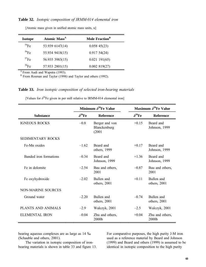
3

4

weight values adopted at the 41st IUPAC General Assembly in Brisbane in July 2001 are listed instead. For most elements, data are graphically illustrated by a diagram in which the materials are specified in the ordinate and the compositional ranges are plotted along the abscissa on three scales: atomic weight, mole fraction of a selected isotope, and relative isotope ratio expressed as deviation from the isotope ratio of a reference in parts per thousand. The mole fraction of a selected isotope is given in percent in figures, tables, and text in this report. Mole fractions of the selected isotope are calculated from the relative isotope ratio by using the absolute isotope-abundance measurement of the reference for the delta scale. Atomic-weight values are calculated from atomic masses and mole fractions of the isotopes, assuming mass-dependent fractionation among the isotopes. The three scales are related exactly for elements with two isotopes for which absolute isotope abundances of the references are known; however, the scales may be mismatched in some cases: (1) for some elements, the absolute isotope abundances of the reference may not be known to within the precision of the common relative isotope-ratio measurements, (2) calculations of atomic weights for polyisotopic elements are subject to additional, usually negligible, adjustments based either on additional abundance measurements or on an assumption about the mass-dependent fractionation of isotopes that are not commonly measured. The section for each element lists the isotopic composition of a real or hypothetical material with delta value of 0 ‰; commonly, this material has been used for the best absolute isotope-abundance measurement as reported by Rosman and Taylor (1998). For many elements the atomic weight derived from the best measurement is not exactly the same as the standard atomic weight. This difference results because (1) the standard atomic weight uncertainty is limited to a single digit and the two cannot match exactly, or (2) Ar(E) was assigned to be in the center of a range of natural isotopic variation and may be greatly different than that of the best measurement substance. With the proliferation of microprobe techniques for isotope measurements, large variations in isotopic composition have been found in source materials over distances of the order of 1 to 1000 μm (McKibben and Eldridge, 1994). Such data are excluded from this compilation, as are data from extraterrestrial materials. Although the data presented in this report may allow reduction in the uncertainty in atomic weight of a substance, the reader is warned that when critical

work is undertaken, such as assessment of individual properties, samples with accurately known isotope abundances should be obtained or suitable measurements made. Acknowledgments Dr. Michael Wieser (University of Calgary, Calgary, Alberta, Canada), Dr. Thomas Walczyk (Swiss Federal Institute of Technology, Rüschlikon, Switzerland), and Ms. Kathryn Plummer are thanked for their reviews of this document, which improved it greatly. The authors are indebted to Prof. Donald J. DePaolo (University of California, Berkeley, California) for calcium isotope-ratio measurements of NIST SRM 915 and NIST SRM 915a calcium carbonate that allow us to correlate the δ44Ca scale to the absolute 44Ca scale. Dr. Roland A. Werner (Max-Planck-Institute for Biogeochemistry, Jena, Germany) is thanked for providing isotope data for this report. Dr. Christina L. De La Rocha (University of Cambridge, Cambridge, United Kingdom) provided comments on the calcium and silicon isotopic sections. Prof. T. M. Johnson (University of Illinois at Urbana-Champaign, Illinois) kindly provided chromium isotope data for this project. Prof. M. Whiticar (University of Victoria, Victoria, British Columbia, Canada) is thanked for the information on extreme isotope ratios he provided for this project. Dr. Thomas D. Bullen (U.S. Geological Survey) is thanked for helpful discussions, which improved this report substantially. Ms. I. Hamblen, Ms. M. Shapira, Ms. Shalini Mohleji, and Ms. Michelle Gendron are thanked for exhaustive library work. Dominion Semiconductor, Manassas, Virginia, is thanked for providing a sample of high purity elemental silicon for isotope-ratio analysis. Hydrogen Ar(H) = 1.00 794(7) Hydrogen is the third most abundant element on surface of the Earth (after oxygen and silicon), and hydrogen in combined form accounts for about 15.4 % of the atoms in the Earth’s crust (Greenwood and Earnshaw, 1997). Most (97 %) of the hydrogen produced in industry is produced on site as needed, for example, for ammonia synthesis, petrochemical uses, and other uses (Greenwood and Earnshaw, 1997). In additional, large quantities of hydrogen are produced for general use (~6.5 × 1010 g3 in the United States alone).

5

Reference materials and reporting of isotope ratios The primary isotopic reference material for hydrogen-bearing materials is the IAEA (International Atomic Energy Agency) reference water VSMOW (Vienna Standard Mean Ocean Water), which is assigned a δ2H value of 0 ‰. Since 1993, CAWIA has recommended (Coplen, 1994) that stable hydrogen relative isotope ratios be reported relative to VSMOW (also distributed by NIST as RM 8535) on a scale normalized by assigning a δ2H value of –428 ‰ to the IAEA reference water SLAP (Standard Light Antarctic Precipitation), which also is distributed as NIST RM 8537. Sometimes δ2H is designated δD in the literature. Hydrogen isotopic compositions are determined on gaseous hydrogen using electron impact ionization mass spectrometry and commonly are measured with a 1-σ standard deviation of ±1 ‰. The absolute hydrogen isotope abundances of VSMOW reference water have been measured by Hagemann and others (1970), De Wit and others (1980), and Tse and others (1980), and a weighted mean value is shown in table 1. One water (GISP), 1 oil (NBS 22), 1 biotite (NBS 30), 1 polyethylene foil (PEF1, renamed IAEA-CH-7), and 3 natural gases (NGS1, NGS2, and NGS3) are secondary reference materials distributed by IAEA and (or) NIST (table 2). In addition, for tracer studies the IAEA distributes IAEA-302A water with δ2H of +508.4 ‰ and IAEA-302B water with δ2H of +996 ‰ (Parr and Clements, 1991). Ranges in Isotopic Composition Hydrogen has the largest relative mass difference among its isotopes and consequently exhibits the largest variation in isotopic composition of any element that does not have radioactive or radiogenic isotopes. Ranges in the stable isotopic composition of naturally occurring hydrogen-bearing materials are shown in table 3 and figure 1. Compilations of

hydrogen isotopic variations and isotope-fractionation factors include Friedman and O'Neil (1977; 1978), Fritz and Fontes (1989), Clark and Fritz (1997), and Valley and Cole (2001). Water Variations in the 2H content of surface waters, ground waters, and glacial ice generally are concordant with δ18O variations and are caused primarily by evaporation and condensation processes (IAEA, 1981). Atmospheric moisture is depleted in 2H by about 100 ‰ at 5°C relative to precipitation. The δ2H values of naturally occurring waters range from –495 ‰ in Antarctic ice (Jouzel and others, 1987) to +129 ‰ in the Gara Diba Guelta Basin of the northwestern Sahara (Fontes and Gonfiantini, 1967). In precipitation δ2H values decrease with increasing latitude, distance inland from a coast (Dansgaard, 1964), and increasing altitude [on the windward side of mountains only, a typical gradient in δ2H of from –1.5 ‰ to –4 ‰ per 100 m is observed (Yurtsever and Gat, 1981)]. Precipitation is depleted in 2H during winters relative to summers. Glacial-ice cores, studied to determine long-term climate change, typically are depleted in 2H during full-glacial climates relative to interglacial climates. These isotopic variations permit tracing and identification of the origin and history of ground and surface waters (Coplen, 1993; Coplen, 1999). Deep oceanic water nearly is homogeneous in δ2H, varying from –1.7 ± 0.8 ‰ in the Antarctic circumpolar region to +2.2 ± 1.0 ‰ in the Arctic (Redfield and Friedman, 1965). The δ2H values of hydrothermal waters generally are identical to those of cold ground waters entering thermal regimes because there is little hydrogen in rocks to undergo hydrogen exchange. An unusual occurrence of water from a well in the Lacq natural gas field in France yielded δ2H values as high as +375 ‰ (Roth, 1956). This occurrence was caused by a small amount of the water equilibrated at near ambient temperature with a much larger amount of H2S with a δ2H value of –430 ‰. The hydrogen

Table 1. Hydrogen isotopic composition of VSMOW reference water [Atomic mass given in unified atomic mass units, u]

Isotope Atomic MassA Mole FractionB

1H 1.007 825 0319(6) 0.999 844 26(5) 2H 2.014 101 7779(6) 0.000 155 74(5)

A From Audi and Wapstra (1993). B From Rosman and Taylor (1998) and Hagemann and others (1970).

6

Table 2. Hydrogen isotopic composition of selected hydrogen-bearing isotopic reference materials [Values for δ2H given in per mill relative to VSMOW on a scale normalized such that the δ2H of SLAP is –428 ‰ relative to

VSMOW]

Reference Material Substance δ2H Reference

VSMOW water 0 (exactly) Gonfiantini, 1978

GISP water –189.73 ± 0.87 Gonfiantini and others, 1995

SLAP water –428 (exactly) Gonfiantini, 1978

NBS 22 oil –120 ± 4 Hut, 1987

NBS 30 biotite –65.7 ± 0.27 Gonfiantini and others, 1995

NGS1 CH4 in natural gas –138 ± 6 Hut, 1987


NGS2 C2H6 in natural gas –121 ± 7 Hut, 1987


IAEA-CH-7 (PEF1) polyethylene –100.33 ± 2.05 Gonfiantini and others, 1995

isotope-fractionation factor between water and H2S is greater than 2, giving rise to water with a δ2H value of +375 ‰. Experimentally, it is possible to produce δ2H values in excess of +130 ‰ by evaporating water with a fan in a low humidity environment. Most salt hydrates are depleted in 2H relative to the coexisting liquid—for example, by 15 ‰ for gypsum. Some hydrates concentrate 2H; CaCl2⋅6H2O and Na2SO4⋅10H2O are enriched in 2H by 10 ‰ and 17 ‰, respectively (Friedman and O'Neil, 1977; Friedman and O'Neil, 1978). Agricultural food products are influenced by the isotopic composition of local meteoric waters. The enrichment of apple juice in 2H is not as large as that in orange juice because of the lower levels of evapotranspiration occurring in the cooler northern latitudes of apple production. However, citrus trees are found in areas with subtropical climates when evaporation fractionates the water isotopes, resulting in 2H enrichment in cellular water. For example, the 2H content of orange juice is enriched by up to 40 ‰ relative to local meteoric water. Bricout and others (1973; also see Donner and others, 1987) showed that natural orange juice could be distinguished from orange juice reconstituted from concentrate and water added from higher latitudes because such waters

typically are depleted in 2H. The most positive δ2H value for fruit juice and wine (+47 ‰) was reported for a sample of red wine (Martin and others, 1988). Silicates The range of δ2H values of silicates (table 3) is from –429 ‰ (Wenner, 1979) to +5 ‰ (Graham and Sheppard, 1980). Hydrogen isotope fractionations between most hydrogen-bearing minerals and water appear to be largely a function of the mass to charge ratio of the octahedral cation, and most hydrogen-bearing silicates are depleted in 2H by 0 ‰ to 100 ‰. Because local meteoric water is involved in the formation or alteration of most hydrogen-bearing silicates, these silicates show a wide range in δ2H. The extremely low value of δ2H in pectolites [–429 ‰ to –281 ‰; (Wenner, 1979)] is not completely understood, but must result because of an unusual isotope-fractionation factor (Wenner, 1979). Analcime channel waters vary systematically with sample locality, whereas channel water in other zeolites (chabazite, clinoptilolite, laumontite, and mordenite) is largely from the ambient water vapor where the zeolites were last stored (Karlsson and Clayton, 1990). Hydrated silica (opal and diatomite) contains several types of structural water, much of which will be exchanged if temperatures reach 100 °C or at lower temperatures over geologic time.

7

Table 3. Hydrogen isotopic composition of selected hydrogen-bearing materials [Values for δ2H given in per mill relative to VSMOW on a scale normalized such that the δ2H of SLAP is –428 ‰

relative to VSMOW]

Minimum δ2H Value Maximum δ2H Value

Substance δ2H Reference δ2H Reference

WATER

Sea water (deep) –2.5 Redfield and Friedman, 1965

+3.2 Redfield and Friedman, 1965

Other (naturally occurring) –495 Jouzel and others, 1987

+129 Fontes and Gonfiantini, 1967

Fruit juice and wine –43 Bricout and others, 1973

+47 Martin and others, 1988

SILICATES

Ca2NaH(SiO3) (pectolite) –429 Wenner, 1979 –281 Wenner, 1979

Other –208 Friedman and O'Neil, 1978

+5 Graham and Sheppard, 1980

HYDROXIDES

Aluminum and iron –220 Yapp, 1993 –8 Bernard, 1978; Bird and others, 1989

ORGANIC HYDROGEN

Non-marine organisms –237 Schütze and others, 1982

+66 Sternberg and others, 1984

Marine organisms –166 Schiegl and Vogel, 1970

–13 Schiegl and Vogel, 1970

Organic sediments –103 Schiegl, 1972 –59 Oremland and others, 1988a

Coal –162 Smith and Pallasser, 1996

–65 Redding, 1978

Crude oil –163 Schiegl and Vogel, 1970

–80 Schiegl and Vogel, 1970

Ethanol (naturally occurring)

–272 Rauschenbach and others, 1979


Ethanol (synthetic) –140 Rauschenbach and others, 1979


8

Table 3. Hydrogen isotopic composition of selected hydrogen-bearing materials—Continued

Minimum δ2H Value Maximum δ2H Value

Substance δ2H Reference δ2H Reference

METHANE

Atmospheric –232 Snover and others, 2000

–71 Wahlen, 1993

Other (naturally occurring) –531 Oremland and others, 1988b

–133 Schoell, 1980

HYDROGEN GAS

Air –136 Friedman and Scholz, 1974

+180 Gonsior and others, 1966

Other (naturally occurring) –836 Coveney and others, 1987

–250 Friedman and O'Neil, 1978

Commercial tank gas –813 T. B. Coplen, unpublished data

–56 J. Morrison, Micromass UK Ltd., Manchester, U.K., oral communication, 2002

Automobile exhaust and industrial contamination

–690 Gonsior and others, 1966

–147 Gonsior and others, 1966

Hydroxides The δ2H of naturally occurring gibbsite (Al2O3⋅3H2O) and goethite [FeO(OH)] range from –220 ‰ to –8 ‰ (Yapp, 1993; Bernard, 1978) as shown in table 3. Hydroxides formed during much of the Phanerozoic in systems such as lateritic paleosols, bog ores, and other materials. Stable hydrogen and oxygen isotope ratios of hydroxides in these systems may provide information on continental paleoclimates (Yapp, 1993; Bird and others, 1989). Organic hydrogen The hydrogen isotopic composition of organisms primarily reflects the hydrogen isotopic composition of water in the local environmental. Trees acquire their n(2H)/n(1H) ratios from precipitation or (and) ground water. The large range in δ2H of meteoric water gives rise to the large variation in δ2H of vegetation (Yapp and Epstein, 1982) shown in table 3. The δ2H values of sap from different types of trees range from –66 ‰ to –1 ‰ (White and others, 1985) with an anomalous value of +60 ‰ for sap from a poplar tree (Schiegl and Vogel, 1970). Evaporation and species-specific variations during metabolic or biochemical processes affect the hydrogen isotopic composition of organisms (Sternberg, 1988). The hydrogen isotopic composition of cellulose can be used to distinguish

plants using the CAM photosynthetic pathway (δ2H = +51 ± 10 ‰) from those using C3 and C4 pathways (δ2H = –40 ± 20 ‰) according to Sternberg and others (1984). Zhang and others (1994) investigated the site-specific natural isotope fractionation of hydrogen in glucose and find that δ2H values of glucose from C3 plants are more negative (–106 ± 65 ‰) than those in C4 plants (–22 ± 65 ‰); the uncertainty in the difference between the δ2H values they report as ±16 ‰. An example of the practical use of this difference is to identify adulteration of orange juice with beet sugar (Donner and others, 1987). The organism with the lowest 2H content found in the literature is algae from Lake Pomornika, Antarctica, with a δ2H value of –237 ‰ (Schütze and others, 1982). The cellulose of Yucca torreyi has the highest 2H content found in the literature (δ2H = +66 ‰; Sternberg and others, 1984). Marine organisms show a smaller range in δ2H value of between –166 ‰ and –13 ‰ (Schiegl and Vogel, 1970). The δ2H values of organic sediments range between –103 ‰ (Schiegl, 1972) and –59 ‰ (Oremland and others, 1988a). The variation of δ2H in coals—thought to be attributable to differing origins, maturation histories, moisture content during

STANDARD ATOMIC WEIGHT

WATER Sea water (deep) Other (naturally occurring) Fruit juice and wine

SILICATES Ca2NaH(SiO3) (pectolite) Other

HYDROXIDES Aluminum and iron

ORGANIC HYDROGEN Non-marine organisms Marine organisms Organic sediments Coal Crude oil Ethanol (naturally occurring) Ethanol (synthetic)

METHANE Atmospheric Other (naturally occurring)

HYDROGEN GAS Air Other (naturally occurring) Commercial tank gas Auto exhaust & industrial contamination

-1000 -800 -600 -400 -200 0 200

δ2H, in ‰ relative to VSMOW

VSMOWGISPSLAP

NBS 22

NGS1

NGS3

NGS2

NBS 30

0.00000 0.00004 0.00008 0.00012 0.00016Mole Fraction of 2H

1.00785 1.00790 1.00795 1.00800Atomic Weight

Figure 1. Hydrogen isotopic composition and atomic weight of selected hydrogen-bearing materials. The δ2H scale and 2H mole-fraction scale were matched using the data in table 1; therefore, the uncertainty in placement of the atomic-weight scale and the 2H mole-fraction scale relative to the δ2H scale is equivalent to ±0.3 ‰. growth, and plant type—ranges from –162 ‰ (Smith and Pallasser, 1996) to –65 ‰ (Redding, 1978). Crude oil deuterium distributions (table 3) range in δ2H from –163 ‰ to –80 ‰ (Schiegl and Vogel, 1970) with differences between the paraffin fraction and the aromatic fraction. Hydrogen isotope ratios have been successfully

used in food and beverage authentication. Rauschenbach and others (1979) note that ethanol produced from naturally occurring materials has a δ2H ranging between –272 ‰ and –200 ‰ and is easily distinguished from synthetic ethanol, which has δ2H values ranging between –140 ‰ and –117 ‰. According to K.P. Hom (Liquor Control Board of

9

10

Ontario, Ontario, Canada, written communication, 2001), ethanol from pure malt whisky ranges in δ2H from –265 ‰ to –250 ‰ and bourbon is about –225 ‰. The δ2H of amyl alcohol in pure malt whisky is similar to that of ethanol; however, in bourbon the δ2H of amyl alcohol and isobutanol are about –190 ‰ and –165 ‰, respectively. Even in pure malt products, the δ2H of isobutanol is relatively positive (–200 ‰). The major component of mustard oil is allyl isothiocyanate, which can be synthesized at a much lower price than its cost when extracted from mustard seeds; therefore, adulteration of natural mustard oil by adding synthetic allyl isothiocyanate is very profitable (Remaud and others, 1997). Natural and synthetic allyl isothiocyanate can be distinguished by site-specific hydrogen isotope-ratio studies because the δ2H of the hydrogen atoms attached to the terminal carbon of the allyl group are depleted in 2H by more than 150 ‰ than hydrogen in other positions (Remaud and others, 1997). Methane The δ2H of methane in terrestrial materials varies between –531 ‰ and –71 ‰ (table 3). The two major methane production processes are (1) diagenesis of organic matter by bacterial processes, and (2) thermal maturation of organic matter. Biogenic methane, produced by bacterial processes during the early stages of diagenesis, is formed in freshwater and marine environments, recent anoxic sediments, swamps, salt marshes, glacial till deposits, and shallow dry-gas deposits. Marine biogenic methane δ2H values range from –250 ‰ (Nissenbaum and others, 1972) to –168 ‰ (Whiticar and others, 1986), whereas methane in freshwater sediments and swamps is more depleted in 2H and ranges in δ2H from –400 ‰ to –224 ‰ (Whiticar and others, 1986). According to Schoell (1980) and Whiticar and others (1986), methane resulting from acetate fermentation will be depleted in 2H relative to that produced when CO2 reduction predominates (Schoell, 1980; Whiticar and others, 1986) because the fractionation is larger for acetate fermentation due to the transfer of the methyl group during methanogenesis that is depleted in deuterium and accounts for three-fourths of the hydrogen in the methane. The δ2H of thermogenic methane not associated with oil genesis ranges from –177 ‰ to –133 ‰ (Schoell, 1980). The δ2H of thermogenic methane that is associated with oil generation ranges from –495 ‰ (Gerling and others, 1988) to –153 ‰ Schoell (1980). The global average δ2H of atmospheric methane, which originates from swamps, rice paddies,

ruminants, termites, landfills, fossil-fuel production, and biomass burning, is –86 ± 3 ‰ (Quay and others, 1999). Brazilian biomass burning produced methane as negative in δ2H value as –232 ‰ (Snover and others, 2000). Hydrocarbons are formed by a process termed “bit metamorphism” during conventional well drilling, during drilling of ultra-deep gas exploration wells, and during drilling of hard crystalline rocks. Methane produced in this way commonly is substantially depleted in 2H. For example, Whiticar (1990) reports a δ2H value of –760 ‰ for methane from a pilot gas well in Siljan Ring, Sweden. Hydrogen gas The δ2H value of naturally occurring gaseous hydrogen (see table 3) ranges from –836 ‰ in natural gas from a Kansas well (Coveney and others, 1987) to +180 ‰ in atmospheric hydrogen (Gonsior and others, 1966). The 2H content of atmospheric hydrogen can be much higher than in any of its sources. These high concentrations are attributed to the large kinetic isotope-fractionation factor (1.65 ± 0.05) in the reaction of atmospheric hydrogen with HO: H2 + HO → H2O + H, which preferentially enriches remaining hydrogen in 2H (Ehhalt and others, 1989). Low temperature serpentinization of ophiolitic rocks generates free hydrogen along with minor amounts of methane and ethane. Fritz and others (1992) found δ2H values of gaseous hydrogen as negative as –733 ‰. Anthropogenic hydrogen commonly is generated by automobile exhaust, and δ2H values ranges from –690 ‰ to –147 ‰ (Gonsior and others, 1966). The majority of industrial hydrogen is produced from petrochemicals. The dominant process is the catalytic steam-hydrocarbon reforming process using natural gas or oil-refinery feedstock, which typically yields hydrogen that is strongly depleted in 2H (for example, δ2H = –600 ‰). The tank hydrogen with the lowest reported 2H content was from MG Industries and had a δ2H value of –813 ‰. Hydrogen produced by electrolysis constitutes about 4 percent of industrial production and is variable in isotopic composition, but often it only is slightly depleted in 2H relative to feed water (for example, δ2H = –56 ‰; J. Morrison, Micromass UK Ltd., Manchester, U.K., oral communication, 2002). A hydrogen generator can be used to generate hydrogen of a desired isotopic composition by mixing 2H2O into the feed water, as necessary.

11

The lowest reported 2H concentration in a naturally occurring terrestrial material is from hydrogen gas with a δ2H value of –836 ‰, discussed above (Coveney and others, 1987). For this specimen, the mole fraction of 2H is 0.000 0255 and Ar(H) = 1.007 851. The highest reported 2H concentration in a naturally occurring terrestrial material is from atmospheric hydrogen gas with a δ2H value of +180 ‰, discussed above (Gonsior and others, 1966). For this specimen, the mole fraction of 2H is 0.000 1838 and Ar(H) = 1.008 010. Lithium Ar(Li) = 6.941(2) Lithium is about 10,000 times less abundant on Earth than silicon, and about 10–9 as abundant as hydrogen in the cosmos. Lithium is an important industrial compound in lubricating greases, aluminum alloys, brazing flux, and batteries. Lithium carbonate is the most important industrial compound of lithium and is the starting point for the production of most other lithium compounds (Greenwood and Earnshaw, 1997). Reference materials and reporting of isotope ratios The primary reference for the relative isotope abundance measurements of lithium isotopes is the IAEA isotopic reference material L-SVEC (NIST RM 8545), a Li2CO3 with an assigned δ7Li value of 0 ‰. Lithium isotope-ratio measurements commonly are performed using positive ion thermal ionization mass spectrometry, and isotope ratios commonly are determined with a 1-σ standard deviation of ±1 ‰. The absolute isotope abundances of L-SVEC have been measured by Qi and others (1997a) and are shown in table 4. In accord with the recommendation of IUPAC (Coplen, 1996), δ7Li values (based on n(7Li)/n(6Li) measurements) are presented in this

report, though δ6Li values (based on n(6Li)/n(7Li) measurements also have been reported in the literature. IRMM-015 and IRMM-016 lithium carbonates are internationally distributed reference materials that are available from the Institute of Reference Materials and Measurements in Geel, Belgium. The δ7Li of IRMM-015 and IRMM-016, respectively, are –996 ‰ and 0 ‰. Within analytical uncertainty, IRMM-016 has isotope abundances identical to that of L-SVEC (Qi and others, 1997a). Ranges in Isotopic Composition Even though lithium occurs only in the +1 valence state in naturally occurring materials, lithium shows a range in δ7Li of more than 50 ‰. Ranges in stable isotopic composition of naturally occurring lithium-bearing materials are shown in table 5 and figure 2. Marine sources Lithium is supplied to the ocean primarily from two sources: (1) high temperature (> 250 °C) basalt-ocean-water reactions (Edmond and others, 1979), and (2) river input of weathering continental crust. Removal processes of lithium from the ocean include (1) low temperature (< 250°C) alteration of oceanic crust in which basalts take up lithium, (2) biogenic carbonate production—marine carbonates contain 2 mg/kg lithium on average, (3) biogenic opal and chert production—Quaternary radiolarian and diatomaceous oozes contain about 30 mg/kg Li, and (4) diagenesis of clay minerals and authigenic clay mineral production may be the most important sink for lithium (Chan and others, 1992). Sea water is approximately homogeneous and has a δ7Li value of about +33 ‰ (table 5). Using an improved procedure, You and Chan (1996) have been able to improve lithium isotope-ratio precision and reduce the amount of sample required for analysis. The δ7Li of pore water from 195.7 m below the ocean

Table 4. Lithium isotopic composition of L-SVEC lithium carbonate [Atomic mass given in unified atomic mass units, u]


6Li 6.015 1223(5) 0.075 91(20) 7Li 7.016 0041(5) 0.924 09(20)

A From Audi and Wapstra (1993). B From Rosman and Taylor (1998) and Qi and others (1997a).

12

Table 5. Lithium isotopic composition of selected lithium-bearing materials [Values for δ7Li given in per mill relative to L-SVEC]

Minimum δ7Li Value Maximum δ7Li Value

Substance δ7Li Reference δ7Li Reference

MARINE SOURCES

Sea water +32.4 You and Chan, 1996 +33.9 Chan and Edmond, 1988

Hydrothermal fluids +2.6 Chan and others, 1994 +11 Chan and others, 1993

Foraminifera and carbonate sediments

–10 Hoefs and Sywall, 1997 +42 Hoefs and Sywall, 1997

Brines and pore water

+1 Vocke and others, 1990 +56.3 You and Chan, 1996

NON-MARINE SOURCES

Surface water +15.5 Chan and others, 1992 +34.4 Chan and Edmond, 1988

Ground and thermal water

–19 T. Bullen, U.S. Geological Survey, written communication, 2001

+10 T. Bullen, U.S. Geological Survey, written communication, 2001

Contaminated ground water



LITHIUM IN ROCKS

Basalt (unaltered) +3.4 Chan and others, 1992 +6.8 Chan and others, 1992

Basalt (altered) –2.1 Chan and others, 1992 +13.5 Chan and others, 1995

Rhyolite –3.5 Bullen and Kharaka, 1992 –3.5 Bullen and Kharaka, 1992

Granite 0.0 R. D. Vocke, Jr., unpublished data

+11.2 Tomascak and others, 1995

Limestone –3.5 Bullen and Kharaka, 1992 +33.5 Hoefs and Sywall, 1997

PHOSPHATES

LiAlFPO4 (amblygonite)

–13 Cameron, 1955 +7.4 Svec and Anderson, 1965

SILICATES

LiAl(SiO3)2 (spodumene)

–12.6 Cameron, 1955 +11.8 R. D. Vocke, Jr., unpublished data

KLiAl2Si3O10 (lepidolite)

–6.6 Cameron, 1955 +7.2 Cameron, 1955

13

Table 5. Lithium isotopic composition of selected lithium-bearing materials—Continued

Minimum δ7Li Value Maximum δ7Li Value

Substance δ7Li Reference δ7Li Reference

REAGENTS 6Li depleted

compounds +434 Qi and others, 1997a +3013 Qi, and others, 1997a

Other –11 Qi and others, 1997a +23 Qi, and others, 1997a

bottom at ODP site 851A contains the highest level of 7Li recorded in a natural terrestrial sample, with δ7Li = +56.3 ‰ (You and Chan, 1996). The mole fraction of 7Li in this specimen is 0.9278 and Ar(Li) = 6.9438. The δ7Li of carbonate from the same level was about +33 ‰. Foraminifera shells from ODP site 806B showed a δ7Li value of about +40 ‰. The foraminiferal lithium isotope data of You and Chan (1996) indicate glacial-interglacial changes in the inventory and isotopic composition of oceanic lithium. Four samples of foraminiferal tests from 2 glacial-interglacial cycles during the past 1 million years show systematic variations of lithium content and lithium isotope abundances with climate. Non-marine sources In order to understand the global lithium cycle, Chan and others (1992) analyzed the δ7Li values of rivers in different geologic terrains. Not surprisingly, the δ7Li values of rivers are correlated to geologic terrains of drainage basins. The Mississippi River drains mixed volcanic and sedimentary terrains with a δ7Li value as low as +15.5 ‰. Values as high as +19 ‰ are expected in such terrains. The Amazon River is low in lithium concentration and δ7Li values reach values as high as +30.3 ‰, probably because the ancient shield terrains in this river basin have been almost completely weathered and most of the dissolved lithium is derived from marine evaporites, which are abundant in the Andes Mountains (Chan and others, 1992; Stallard and Edmond, 1983). The lithium isotope abundances of thermal waters are related to geologic environment. Bullen and Kharaka (1992) analyzed thermal waters in Yellowstone National Park and found a wide range in δ7Li value, from –12 ‰ to +2 ‰. Thermal waters from the Norris-Mammoth corridor had similar δ7Li values, whereas thermal waters to the north were enriched in 7Li. These differences are attributed to lower δ7Li values from hydrothermally

altered rocks and the higher δ7Li values being derived from clays and other secondary minerals in marine sediments (Bullen and Kharaka, 1992). The lowest δ7Li value in a natural sample of terrestrial origin is –19 ‰ for a ground water from a coastal aquifer of South Carolina (USA) (T. Bullen, U.S. Geological Survey, written communication, 2001). The mole fraction of 7Li in this ground water is 0.9227 and Ar(Li) = 6.9387. Down gradient in the aquifer, the δ7Li value increased to +10 ‰ after extensive dissolution of marine aragonite, but prior to major Ca-for-Na exchange on clays, which subsequently lowers δ7Li value to approximately 0 ‰. T. Bullen (U.S. Geological Survey, written communication, 2001) reports δ7Li values from –4 ‰ to +354 ‰ in ground water underlying West Valley Creek in Pennsylvania (USA), down gradient from a lithium processing plant. Values as high as +290 ‰ were measured in the main stem of West Valley Creek. The highest values of 7Li content are probably related to removal of 6Li from reagents for use in hydrogen bombs. The remaining lithium is substantially enriched in 7Li and has been used in chemical and pharmaceutical manufacturing. Lithium in rocks In order to investigate the possibility of utilizing lithium isotope ratios between co-precipitating minerals in a granite-pegmatite system, Tomascak and others (1995) analyzed lithium isotope ratios in various pegmatite albites. Wall zone albite was found to be the most enriched in 7Li, but intermediate zones did not show a trend with decreasing temperature of precipitation. Limestone shows a wide variation in δ7Li value with values ranging from –3.5 ‰ in Paleozoic limestone in Yellowstone National Park, Wyoming (Bullen and Kharaka, 1992) to +33.5 ‰ in German limestone (Hoefs and Sywall, 1997). Phosphates Amblygonite (LiAlFPO4) is found in granite pegmatite and is mined as an ore of lithium.


MARINE SOURCES Sea water Hydrothermal fluids Foraminifera and carbonate sediments Brines and pore water

NON-MARINE SOURCES Surface water Ground and thermal water Contaminated ground water

LITHIUM IN ROCKS Basalt (unaltered) Basalt (altered) Rhyolite Granite Limestone

PHOSPHATES LiAlFPO4 (amblygonite)

SILICATES LiAl(SiO3)2 (spodumene) KLiAl2Si3O10 (lepidolite)

REAGENTS 6Li depleted compounds Other

-20 -10 0 10 20 30 40 50 60

δ7Li, in ‰ relative to L-SVEC

L-SVEC IRMM-016

to +354

+434 to +3013

6.938 6.939 6.940 6.941

Atomic Weight6.942 6.943 6.944

0.923 0.924 0.925Mole Fraction of 7Li

0.926 0.927 0.928

Figure 2. Lithium isotopic composition and atomic weight of selected lithium-bearing materials. The δ7Li scale and 7Li mole-fraction scale were matched using the data in table 4; therefore, the uncertainty in placement of the atomic-weight scale and the 7Li mole-fraction scale relative to the δ7Li scale is equivalent to ±3 ‰. Published δ7Li values of amblygonite range from –13 ‰ (Cameron, 1955) to +7.4 ‰ (Svec and Anderson, 1965). Silicates Li-bearing silicates were among the first Li-bearing specimens to be analyzed for lithium isotopic composition. The δ7Li of spodumene ranges between –12.6 ‰ (Cameron, 1955) and +11.8 ‰ (R. D. Vocke, Jr., unpublished data). That of lepidolite ranges between –6.6 ‰ and +7.2 ‰ (Cameron, 1955).

Reagents Of the chemical elements discussed in this report, lithium is particularly unusual because large amounts of lithium have been isotopically fractionated by removal of 6Li for use in hydrogen bombs. The remaining lithium is substantially enriched in 7Li and some of this lithium has found its way into laboratory reagents and into the environment. An analysis of 39 laboratory reagents (Qi and others, 1997b) indicated a δ7Li range of

14

15

between –11 ‰ (for Baker-Adamson lithium sulfate) and +3013 ‰ (for Fisher Scientific lithium hydroxide). The δ7Li of lithium carbonate, the most common starting material for other Li-bearing reagents, ranged from 0 ‰ to +12 ‰. Boron Ar(B) = 10.811(7) Boron is not abundant—its average concentration in crustal rocks (9 mg/kg) is less than that of lithium (18 mg/kg). A primary commercial source is borate minerals found in commercial quantities in California (USA) and Turkey. 10B is used in nuclear applications in neutron shields and control rods because of the high absorption cross-section of 10B for thermal neutrons. The primary non-nuclear uses of boron are in heat resistant glasses (Pyrex), detergents, soaps, cleaners, cosmetics, porcelain enamels, synthetic herbicides and fertilizers, and abrasives. Reference materials and reporting of isotope ratios The primary reference for the relative abundance measurements of boron isotopes is the NIST reference material SRM 951 boric acid, which is assigned a δ11B value of 0 ‰. Boron isotope-ratio measurements commonly are performed using negative ion thermal ionization mass spectrometry, and isotope ratios commonly are determined with a 1-σ standard deviation of ±1 ‰. The absolute isotope abundances of SRM 951 have been measured by Catanzaro and others (1970) and are listed in table 6. A second reference material, IRMM-011 boric acid, is nearly identical in isotopic composition to SRM 951 (NIST, 1999a), and it is available from IRMM (Institute for Reference Materials and Measurements), Geel, Belgium. Two boric acid reference materials (IRMM-610 and SRM 952) are depleted in 11B (NIST, 1999b; IRMM, 2001).

The IAEA recognized the paucity of boron isotopic reference materials and has recently distributed 3 water and 5 rock reference materials to boron isotope laboratories (Tonarini and others, in press). These materials have been analyzed by negative ion thermal ionization mass spectrometry, positive ion thermal ionization mass spectrometry, inductively coupled plasma mass spectrometry, and MC-ICP-MS. These materials are listed in table 7 and shown in fig 3. Ranges in Isotopic Composition Boron isotope ratios show large variations (> 90 ‰) in the terrestrial environment (table 8 and figure 3). Naturally occurring boron predominantly is found in the +3 oxidation state and does not undergo redox reactions. In solution, boric acid is enriched in 11B by 20 ‰ relative to coexisting borate ions, B(OH)4

–. During precipitation, borate preferentially enters the solid phase, enriching the residual solution in 11B. When boron is attracted to clays or other active surfaces, the predominant species attracted is tetrahedral B(OH)4

–; thus, residual dissolved boron is enriched in 11B. Bassett (1990) has compiled and critically evaluated boron isotopic measurements prior to 1990. Marine sources The δ11B of sea water is relatively constant at +39.5 ‰. The values of sea water measured by Schwarcz and others (1969) have not been used because they probably are too high according to Bassett (1990). Shima's (1962; 1963) analyses of borax and ocean water differ by more than 30 ‰ from those of other researchers; thus, they are not included in this report. As sea water evaporates, salts are depleted in 11B by 30 per mill in the early stages of precipitation and by 20 per mill in the latter stages of precipitation (Vengosh and others, 1992), increasing the 11B content of evaporated sea water. The highest published δ11B value of evaporated sea water is +58.5 ‰ from the Mediterranean Sea (Klötzli, 1992).

Table 6. Boron isotopic composition of NIST SRM 951 boric acid [Atomic mass given in unified atomic mass units, u]


10B 10.012 9371(3) 0.198 27(13) 11B 11.009 3055(4) 0.801 73(13)

A From Audi and Wapstra (1993). B From Rosman and Taylor (1998) and Catanzaro and others (1970)

16

Table 7. Boron isotopic composition of selected boron-bearing isotopic reference materials [Values for δ11B given in per mill relative to NIST SRM 951 boric acid]

Reference Material

Substance δ11B Reference

SRM 951 boric acid 0 (exactly) Catanzaro and others, 1970

IRMM-011 boric acid –0.16 Lamberty and De Bièvre, 1991

SRM 952 boric acid –987 NIST, 1999b

IRMM-610 boric acid solution –987 IRMM, 2001

IAEA-B-1 surface sea water, Western Mediterranean Sea

+37.7 ± 2.1 Tonarini and others, in press

IAEA-B-2 ground water, alluvial aquifer, Cecina River, lower basin (Tuscany, Italy)


IAEA-B-3 ground water, alluvial aquifer, River Cecina, upper basin (Tuscany, Italy)

–21.3 ± 0.9 Tonarini and others, in press

IAEA-B-4 tourmaline, Elba Island (Tuscan Archipelago, Italy)


IAEA-B-5 basalt, Mt. Etna’s main crater (Sicily), eruption July 1998


IAEA-B-6 obsidian, Lipari Island, Italy (Eolian Archipelago)


IAEA-B-7 Miocene marine limestone (Abruzzi, Italy)


IAEA-B-8 Pliocene clay (Montelupo Fiorentino, Italy)


Large-scale boron exchange between sea water and oceanic crust occurs at both high and low temperature (Spivack and Edmond, 1987). Hydrothermal solutions from 9 separate oceanic vent fields have δ11B values between +30.0 ‰ and +36.8 ‰ (Spivack and Edmond, 1987). Boron extracted from basalts involved in high temperature reaction show no resolvable isotope fractionation. Serpentinites and basalts altered at low temperature are enriched in boron and have δ11B values between +0.1 ‰ and +9.2 ‰. This preferential transfer of 10B into altered oceanic sediments is in part responsible for the high δ11B of sea water. Because the δ11B of sea water is about +40 ‰ and because the isotope fractionation between B(OH)3 and B(OH)–

4 is about 20 ‰ (Kakihana and others, 1977), the δ11B of marine evaporites should be about

+20 ‰ or higher. Swihart and others (1986) find the range to be between +18.2 ‰ and +31.7 ‰. The δ11B of modern marine carbonates falls in a relatively narrow range (+22 ± 3 ‰) according to Hemming and Hanson (1992). This band is about 20 ‰ more negative than that of sea water and is explained by the fact that tetrahedral B(OH)–

4, which is depleted in 11B by 20 ‰ relative to B(OH)3, is preferentially incorporated into the carbonate structure. The range in δ11B value expands from +4.0 ‰ to +32.2 ‰ (Vengosh and others, 1991b) if hand picked foraminifera and ostracoda are included. Non-marine sources The primary sources of boron are non-marine evaporite deposits in California (USA) and Turkey, which yield large quantities of borates. It was hypothesized that non-marine borates would reflect the isotopic composition of crustal rocks

17

Table 8. Boron isotopic composition of selected boron-bearing materials [Values for δ11B given in per mill relative to NIST SRM 951 boric acid]

Minimum δ11B Value Maximum δ11B Value

Substance δ11B Reference δ11B Reference

MARINE SOURCES

Sea water +38.4 Vengosh and others, 1991a

+40.4 Nomura and others, 1982

Evaporated sea water +36.5 Vengosh and others, 1991a

+58.5 Klötzli, 1992

Hydrothermal fluids +30.0 Spivack and Edmond, 1987

+36.8 Spivack and Edmond, 1987

Evaporite minerals +18.2 Swihart and others, 1986

+31.7 Swihart and others, 1986

Carbonates (Skeletal parts and formations)

+4.0 Vengosh and others, 1991b

+32.2 Vengosh and others, 1991b

NON-MARINE SOURCES

Rain water +0.8 Spivack, 1986 +35 Spivack, 1986

Brines, surface and ground waters

–21.3 Tonarini and others, in press

+59.2 Vengosh and others, 1991a

Hydrothermal fluids –9.3 Palmer and Sturchio, 1990

+29.1 Klötzli, 1992

Evaporite minerals –31.3 Finley and others, 1962

+7.3 Agyei and McMullen, 1968

IGNEOUS ROCKS –17.0 Trumbull and Chaussidon, 1999

–1.7 Spivack and Edmond, 1987

METAMORPHIC ROCKS –34.2 Wang and Xiao, 2000

+22 Swihart and Moore, 1989

SEDIMENTS –17 Ishikawa and Nakamura, 1993

+26.2 Ishikawa and Nakamura, 1993

ORGANIC BORON –12 Wieser and others, 2001

+29.3 Vanderpool and Johnson, 1992

and minerals, which is about 40 ‰ more negative than marine boron (Swihart and others, 1986). Except for one value at +24 ‰, the δ11B of non-marine evaporites ranged between –31.3 ‰ (Finley and others, 1962) and +7.3 ‰ (Agyei and McMullen, 1968). Thus, non-marine borates are depleted in 11B relative to marine borates (+18.2 ‰

to +31.7 ‰) and boron isotope ratios can be used to differentiate the two evaporite borates (Swihart and others, 1986). The boron isotopic composition of fumarolic condensates is thought to reflect the boron isotopic composition of associated magmas (Kanzaki and others, 1979). Nomura and others (1982) measured


MARINE SOURCES Sea water Evaporated sea water Hydrothermal fluids Evaporite minerals Carbonates (skeletal parts and formations)

NON-MARINE SOURCES Rain water Brines, surface and ground waters Hydrothermal fluids Evaporite minerals

IGNEOUS ROCKS

METAMORPHIC ROCKS

SEDIMENTS

ORGANIC BORON

-40 -20 0 20 40 60

δ11B, in ‰ relative to SRM 951

SRM 951IRMM-011

IAEA-B-1

IAEA-B-2IAEA-B-3

IAEA-B-4 IAEA-B-5IAEA-B-6

IAEA-B-7

IAEA-B-8

0.795 0.800Mole Fraction of 11B

10.805 10.810Atomic Weight

0.805 0.810

10.815 10.820

Figure 3. Boron isotopic composition and atomic weight of selected boron-bearing materials. The δ11B scale and 11B mole-fraction scale were matched using the data in table 6; therefore, the uncertainty in the placement of the atomic-weight scale and the 11B mole-fraction scale relative to the δ11B scale is equivalent to ±0.8 ‰. 40 fumarolic condensates from the Japanese island arc. Most condensates possess δ11B values near +6 ‰, reflecting the boron isotopic composition of crustal rocks. However, values above +17 ‰ were found in the southernmost end of the northeastern Japanese arc, and these more positive values were attributed to interaction of magmas with sea water (δ11B = +39.5 ‰). In a reconnaissance of Yellowstone National Park (Wyoming), Palmer and Sturchio (1990) found δ11B values between –9.3 ‰ and +4.4 ‰. They suggest that the most negative values may be explained by leaching of boron from hydrothermally altered rhyolite. The highest δ11B values in hydrothermal fluids were measured by Klötzli (1992) on Larderello geothermal field (Italy)

samples (+21.8 ‰ to +29.1 ‰). These high values were attributed to meteoric waters incorporating boron from marine sediments. The δ11B value of –59 ‰ obtained for Sasso Pisano 6 is not included because it cannot be satisfactorily explained (Klötzli, 1992)—it may be due to matrix effects during the isotopic analysis. An important source of boron to the oceans for studying global boron cycling is boron in rivers. The δ11B values of rivers representing 39 percent of the total world discharge of water range from –5.9 ‰ to +42.8 ‰ (Lemarchand and others, 2000). Surface and ground waters display a wide range in boron isotopic composition. Gäbler and Bahr (1999) were able to confirm the anthropogenic input

18

19

of boron in ground water north of the Harz Mountains in Germany. They identified a region with δ11B values between –3 ‰ and +3 ‰ and attributed these values to perborates in detergents (exactly the range expected for perborates in the United States and Europe). Bassett and others (1995) were able to distinguish water-recharge types in an injection site of treated wastewater into an alluvial aquifer near El Paso, Texas, because the δ11B of native ground water was +14 ‰; that of municipal wastewater was between +6 ‰ and +10 ‰, and that of irrigation-affected water was greater than +40 ‰. The highest δ11B value found in the literature for a naturally occurring terrestrial material is +59.2 ‰ in brine from Maar lakes from southwestern Victoria, Australia (Vengosh and others, 1991a). The mole fraction of 11B in this sample is 0.8107 and Ar(B) = 10.8207. Another continental brine, also of largely marine derived boron, is found in Laizhou Bay region of China with a δ11B value of +57.5 ‰ (Xiao and others, 2001). Both of these brines have non-marine B/Cl ratios. Igneous rocks The δ11B of boron in the mantle is –10 ± 2 ‰, based on measurements of volcanic glasses and oceanic island basalts, which yield δ11B = –9.9 ± 1.3 ‰ (Chaussidon and Marty, 1995). Unaltered mid-ocean ridge basalts from the East Pacific Rise have δ11B values in the range of –4.0 ‰ to –1.7 ‰ (Spivack and Edmond, 1987; Chaussidon and Marty, 1995). As basalts undergo low temperature alteration, 11B and boron concentrations are increased as discussed above. In a study in Swaziland, tourmalines in granite have a narrow range in δ11B of between –17.0 ‰ and –13.5 ‰ (Trumbull and Chaussidon, 1999). In a worldwide survey of boron isotopic composition, Swihart and Moore (1989) observed a range in δ11B of –12 ‰ to –5 ‰ for tourmaline in granite pegmatites. Metamorphic rocks Tourmalines from a coarse, zoned pegmatite and hydrothermal tourmalines in a study from Swaziland ranged in δ11B value from –23.0 ‰ to –16.6 ‰ (Trumbull and Chaussidon, 1999). Swihart and Moore (1989) found a range in δ11B of –22 ‰ to +22 ‰ for tourmalines and metasedimentary rocks. Relatively high concentrations of 11B (δ11B > –1 ‰) were interpreted as indicating boron of marine or sedimentary origin. The sample of natural terrestrial origin with the lowest reported 11B content in figure 3 is kornerupine [(Mg,Fe2+)4(Al,Fe3+)6(SiO4,BO4)5(O,OH)2] from Antarctica (Wang and Xiao, 2000) with a δ11B value of –34.2 ‰. The mole fraction of 11B of this specimen is 0.7961 and Ar(B) = 10.8062.

Sediments The boron isotopic composition of sediments is variable. Boron isotopes are fractionated by 30 ‰ to 40 ‰ by preferential adsorption of 10B of dissolved boron on clay minerals (Schwarcz and others, 1969), giving rise to low δ11B values of clays. The δ11B of most modern marine sediments falls in the range –6.6 ‰ to +4.8 ‰ (Ishikawa and Nakamura, 1993). The boron isotopic composition is controlled by mass balance of four major constituents: detritus of continental origin, marine smectite, biogenic carbonates, and biogenic silica. Detritus of continental origin, especially illite from eolian or fluvial transport, is the low δ11B end-member of marine sediments (–13 ‰ to –8 ‰). Biogenic carbonate is the high end-member with δ11B values between +8.0 ‰ and +26.2 ‰ (Ishikawa and Nakamura, 1993). These high 11B concentrations are the result of equilibrium uptake of boron from sea water. The δ11B of ancient marine sediments is more negative (–17.0 ‰ to –5.6 ‰) than that of modern sediments (Ishikawa and Nakamura, 1993). The more negative δ11B values can be caused by diagenesis, which promotes preferential removal of 11B in calcium carbonate and silica during recrystallization, or by boron isotopic exchange during smectite/illite transition. Organic boron Boron is an essential chemical element for the healthy development of many plants. Vanderpool and Johnson (1992) analyzed a variety of commercial produce grown in North America and found a range of –7.5 ‰ to +29.3 ‰ in δ11B. Wieser and others (2001) analyzed the boron isotopic composition of Coffee arabica bean samples from around the world and found δ11B values from –12 ‰ for Peru “organic” beans to +19 ‰ for beans from Tanzania. Wieser and others (2001) conclude that the isotopic composition of local boron sources, such as boron in the soil, fertilizer, and water, control the δ11B values of the coffee beans. Thus, the boron isotopic composition of coffee can be used in quality-assurance programs as the quality depends to a large extent on the genetic and geographic origin of the coffee. Williams and others (2001) analyzed boron content and isotopic composition of kerogen in Gulf of Mexico sediments. They found large concentrations of organically bound boron (140 mg/kg) with a δ11B value of –2 ‰ that may serve as a source for boron in deep sedimentary brines with low δ11B values (< approximately 25 ‰).

20

Carbon Ar(C) = 12.0107(8) Although carbon is the fourth most abundant element in the universe after hydrogen, helium, and oxygen, its abundance in the Earth’s crust is only about fourteenth. Carbon occurs as the free element (graphite and diamond), in fossil fuels (coal and petroleum), as the important atmospheric gas carbon dioxide, in carbonates of calcium and magnesium, and in living and dead plants and animals. Important uses include energy production, steel making, sugar manufacturing, water treatment, and respirators. The continual interaction of carbon among the lithosphere, biosphere, atmosphere, and hydrosphere is called the carbon cycle. Carbon isotope ratios commonly are used to investigate carbon-cycle processes. Reference materials and reporting of isotope ratios Beginning in the 1950's, isotope-abundance measurements of carbon isotopes were expressed relative to Peedee belemnite (PDB), which was assigned a δ13C value of 0 ‰. Because the supply of PDB is exhausted, IUPAC recommended in 1993 (Coplen, 1994; IUPAC, 1994) that carbon isotope abundances be reported relative to VPDB (Vienna PDB, the new primary reference for carbon isotope ratios having a δ13C value of 0 ‰) by assigning an exact δ13C value of +1.95 ‰ on the VPDB scale to the IAEA reference material NBS 19 calcium carbonate. Carbon isotope ratios are determined on gaseous CO2 using electron impact ionization mass spectrometry and commonly are measured with a 1-σ standard deviation of ±0.1 ‰. The absolute isotope abundances of NBS 19 have been measured by Chang and Li (1990), and they calculated from this measurement the absolute isotope abundances of the zero point of the VPDB scale (table 9).

Secondary reference materials (see table 10) are distributed by IAEA and (or) NIST and include various carbonates, natural gases, sugars, and an oil (Gonfiantini and others, 1995). Reference materials in a subset of these (Parr and Clements, 1991) are variably enriched in 13C and intended for use mainly in medical and biological tracer studies. Ranges in Isotopic Composition Carbon occurs in valence states between +4 and –4 in naturally occurring materials. Therefore, the range in isotopic variation of carbon-bearing materials is greater than 140 ‰ (table 11 and figure 4). Useful compilations of carbon isotopic variations and isotope- fractionation mechanisms include Friedman and O'Neil (1977), Schwarcz (1969), Clark and Fritz (1997) and Valley and Cole (2001). Carbon occurs primarily in 3 reservoirs on Earth, sedimentary organic matter, the biosphere, and sedimentary carbonates. These reservoirs differ in isotopic composition because of different isotope-fractionation mechanisms. Kinetic isotope fractionation associated with photosynthesis preferentially enriches plant material in 12C. This enrichment gives rise to organic sediments, coal, and crude oil with δ13C values near –25 ‰ and sedimentary carbonates near 0 ‰ (figure 4). Carbonate and bicarbonate Total dissolved inorganic carbon (DIC) consists of dissolved bicarbonate, carbonate, and carbon dioxide in aqueous solution. In most settings, such as the Earth's oceans, bicarbonate ion predominates. The primary sources of DIC are atmospheric CO2, dissolution of carbonate, and decay of organic matter. Although the variation in δ13C of ocean water is small, –0.8 ‰ to +2.2 ‰ (Kroopnick, 1985), the variation in deep sea pore waters ranges from –37.1 ‰ (Nissenbaum and others, 1972) to +37.5 ‰ (Claypool and others, 1985), the latter being the highest δ13C value of a naturally

Table 9. Carbon isotopic composition of a material with δ13C = 0 ‰ relative to VPDB

[Atomic mass given in unified atomic mass units, u]


12C 12 u (exactly) 0.988 944(28) 13C 13.003 354 838(5) 0.011 056(28)

A From Audi and Wapstra (1993). B From Chang and Li (1990) and Rosman and Taylor (1998)

21

Table 10. Carbon isotopic composition of selected carbon-bearing isotopic reference materials [Values for δ13C given in per mill relative to VPDB, defined by assigning an exact δ13C value of +1.95 ‰ to NBS 19 carbonate]

Reference Material Substance δ13C Reference

NBS 18 CaCO3 (carbonatite) –5.01 ± 0.06 Stichler, 1995

NBS 19 CaCO3 (marble) +1.95 (exactly) Hut, 1987

IAEA-CO-1 (IAEA C1)

CaCO3 (marble) +2.48 ± 0.03 Stichler, 1995

IAEA-CO-8 (IAEA KST)

CaCO3 –5.75 ± 0.06 Stichler, 1995

L-SVEC Li2CO3 –46.48 ± 0.15 Stichler, 1995

IAEA-CO-9 (IAEA NZCH)

BaCO3 –47.12 ± 0.15 Stichler, 1995

USGS24 C (graphite) –15.99 ± 0.11 Stichler, 1995

NBS 22 oil –29.74 ± 0.12 Gonfiantini and others, 1995

IAEA-C-6 (Sucrose ANU)

sucrose –10.43 ± 0.13 Gonfiantini and others, 1995

NGS1 CH4 in natural gas –29.0 ± 0.2 Hut, 1987

NGS1 C2H6 in natural gas –26.0 ± 0.6 Hut, 1987

NGS1 C3H8 in natural gas –20.8 ± 1 Hut, 1987


NGS2 C2H6 in natural gas –31.7 ± 0.6 Hut, 1987


NGS2 CO2 in natural gas –8.2 ± 0.4 Hut, 1987



IAEA-CH-7 (PEF1)

polyethylene –31.83 ± 0.11 Gonfiantini and others, 1995

NIST RM 8562 CO2 –3.76 ± 0.03 NIST, 1998

NIST RM 8563 CO2 –41.56 ± 0.06 NIST, 1998

NIST RM 8564 CO2 –10.45 ± 0.04 NIST, 1998 occurring terrestrial specimen found in the literature. The mole fraction of 13C in this specimen is 0.011 466 and Ar(C) = 12.011 50. The δ13C values for igneous carbonates

(carbonatites) range from –11.9 ‰ to +3.1 ‰ (Deines and Gold, 1973). A similar range of –11.9 ‰ to +0.2 ‰ usually is measured for carbonates in kimberlites as well (Khar'kiv and

22

Table 11. Carbon isotopic composition of selected carbon-bearing materials [Values for δ13C given in per mill relative to VPDB, defined by assigning an exact δ13C value of +1.95 ‰ to NBS 19

carbonate]

Minimum δ13C Value Maximum δ13C Value

Substance δ13C Reference δ13C Reference

CARBONATE AND BICARBONATE

Sea water –0.8 Kroopnick, 1985 +2.2 Kroopnick, 1985

Other water –37.1 Nissenbaum and others, 1972

+37.5 Claypool and others, 1985

Metamorphic and igneous rock

–11.9 Deines and Gold, 1973

+24.8 Deines, 1968

Typical marine carbonate rock

–6 Land, 1980 +6 Land, 1980

Other carbonate –64.5 Deuser, 1970 +21.1 Deuser, 1970

CARBON DIOXIDE

Air –8.2 Keeling and others, 1989

–6.7 Keeling, 1958

Soil gas –31.0 Aravena and others, 1996

+6.9 Notsu and others, 2001

Volcanic gas –37 Valyayev and others, 1985

+23 Valyayev and others, 1985

Oil, gas, coal, and landfills

–37.6 Wasserburg and others, 1963

+28 Whiticar and others, 1995

Commercial tank gas and reference materials

–54 T. B. Coplen, unpublished data

–28.76 NIST, 1998

OXALATES

CaC2O4⋅xH2O (whewellite)

–31.7 Žák and Skála, 1993

+33.7 Hofmann and Bernasconi, 1998

CARBON MONOXIDE

Air –31.5 Brenninkmeijer, 1993

–22 Stevens and others, 1972

others, 1986; Mitchell, 1989); however, Deines (1968) has reported unusually high values (–10.2 ‰ to +24.8 ‰) for carbonates from a mica peridotite dike near Dixonville, Pennsylvania (USA). Calc- silicate rocks vary between –16 ‰ and +2 ‰ (Schwarcz, 1969). The testae, skeletons, and shells of marine biota

have δ13C values between –12 ‰ and +5.7 ‰ (Weber and Raup, 1966; Lowenstam and Epstein, 1957; Murata and others, 1969). Marine CaCO3 covers a broad δ13C range from –60.6 ‰ (Hathaway and Degens, 1969) to +15.2 ‰ (Murata and others, 1969). “Typical” unaltered marine limestone tends to have δ13C values between –4 ‰ and +4 ‰. Keith

23

Table 11. Carbon isotopic composition of selected carbon-bearing materials—Continued

Minimum δ13C Value Maximum δ13C Value

Substance δ13C Reference δ13C Reference

ORGANIC CARBON

Land plants (C3 metabolic process)

–35 O'Leary, 1988 –21 Smith and Turner, 1975

Land plants (C4 metabolic process)

–16 Smith and Turner, 1975

–9 Smith and Turner, 1975

Land plants (CAM metabolic process)

–34 Deines, 1980 –10 O'Leary, 1988

Marine organisms –74.3 Paull and others, 1985 –2 Schwarcz, 1969

Marine sediments and compounds

–130.3 Elvert and others, 2000

+7 Deines 1980

Coal –30 Deines, 1980 –19 Deines, 1980

Crude oil –44 Sofer, 1984 –16.8 Sofer 1984

Ethanol (naturally occurring)


–10.3 Rauschenbach and others, 1979

ELEMENTAL CARBON

Graphite –41 Deines, 1980 +6.2 Ghent and O'Neil, 1985

Diamonds –34.4 Galimov, 1985 +5 Harris, 1987

ETHANE

Hydrocarbon gas –55.6 Hut, 1987 +6.6 Gerling and others, 1988

METHANE

Air –50.6 Merritt and others, 1995

–39 Bainbridge and others, 1961

Marine and other sources –109 Whiticar and others, 1986

+12.7 Gerling and others, 1988

Fresh water sources –86 Oremland and King, 1989

–50 Whiticar and others, 1986

Commercial tank gas –51 K. Révész, unpublished data

–38 K. Révész, unpublished data

and Weber (1964) determined a mean of +0.56 ‰ for a selected group of 272 marine limestones. Unusual values usually are found in association with organic matter, methane, and (or) sulfur. The carbonate of freshwater brachiopods (Abell,

1985) and mollusks (Keith and others, 1964) have δ13C values between –19.4 ‰ and +7.0 ‰. Land snail shells vary between –12.0 ‰ and +0.5 ‰ (Tamers, 1970; Goodfriend and Magaritz, 1987). Freshwater CaCO3 has δ13C values between –17.7 ‰


CARBONATE & BICARBONATE Sea water Other water Metamorphic & igneous rock Typical marine carbonate rock Other carbonate

CARBON DIOXIDE Air Soil gas Volcanic gas Oil, gas, coal, and landfills Commercial tank gas and reference materials

OXALATES CaC2O4·xH2O (whewellite)

CARBON MONOXIDE Air

ORGANIC CARBON Land plants (C3 metabolic process) Land plants (C4 metabolic process) Land plants (CAM metabolic process) Marine organisms Marine sediments & compounds Coal Crude oil Ethanol (naturally occurring)

ELEMENTAL CARBON Graphite Diamonds

ETHANE Hydrocarbon gas

METHANE Air Marine and other sources Fresh water sources Commercial tank gas

-160 -140 -120 -100 -80 -60 -40 -20 0 20 40

δ13C, in ‰ relative to VPDB

NBS 18

USGS24

NBS 22

NGS1

IAEA-C-6

NGS1NGS2

NGS2

NGS3

NGS2

NBS 19IAEA-CO-9

RM 8563 RM 8562

NGS3

RM 8564

IAEA-CO-1L-SVEC

0.0095 0.0100 0.0105 0.0110 0.0115Mole Fraction of 13C

12.0095 12.0100 12.0105 12.0110 12.0115Atomic Weight

Figure 4. Carbon isotopic composition and atomic weight of selected carbon-bearing materials. The δ13C scale and 13C mole-fraction scale were matched using the data in table 9; therefore, the uncertainty in placement of the atomic-weight scale and the 13C mole-fraction scale relative to the δ13C scale is equivalent to ±2.5 ‰.

24

25

(Clayton and Degens, 1959, as cited in Murata and others, 1969) and +6.3 ‰ (O'Neil and Barnes, 1971). Keith and Weber (1964) measured an unusual value of –24.2 ‰, which they did not include in their mean of –4.93 ‰ for 158 freshwater limestone samples. Dolomite, CaMg(CO3)2, has δ13C values ranging between –64.5 ‰ and +21.1 ‰ (Deuser, 1970). Most platform dolomites have δ13C values within a smaller range between –6 ‰ and +6 ‰ (Land, 1980). Dolomite with unusual isotopic compositions tends to be associated with organic matter or hydrocarbons (Land, 1980). Marbles have δ13C values between about –12 ‰ and +13 ‰ (Palin and Rye, 1987; Baker and Fallick, 1989). Components of human kidney stones have δ13C values between approximately –22 ‰ and –14 ‰ (Krouse and others, 1987a). The common, low temperature mineral, goethite (α-FeOOH), contains small amounts of an Fe(CO3)OH component in apparent solid solution (Yapp, 1987a) with δ13C values between –21.7 ‰ and +3.3 ‰. Carbon dioxide The N2O-corrected δ13C values of “global” atmospheric CO2 ranged from –8.2 ‰ to –7.0 ‰ during the years from 1977 to 1988 (Mook, 1986; Keeling and others, 1989). A range of –7.5 ‰ to –6.7 ‰ was measured in 1956 (Keeling, 1958). The air samples were collected at sites where industrial and photosynthetic processes have a minimal effect. Two principal global trends have been observed: a long-term gradual decrease in δ13C values and much larger seasonal fluctuation. In both trends, δ13C values tend to decrease with increasing CO2 concentrations (Keeling and others, 1984). The gradual δ13C decrease seems to be primarily because of fossil-fuel combustion (Mook, 1986). Relative to atmospheric CO2, the released CO2 is depleted in 13C (estimated average δ13C values = –27 ‰) reflecting its sources (Tans, 1981). Keeling and others (1979) noted a 0.55 ‰ decrease over the 22-year period from 1956 to 1978; the mean, seasonally adjusted δ13C value changed from –6.7 ‰ to –7.2 ‰ as the CO2 concentration increased from 314 mg/kg to 334 mg/kg in the Northern Hemisphere. Cement use and production also may make a minimal contribution of CO2 with approximate δ13C values of –15 ‰ and +1 ‰, respectively (Mook, 1986). The yearly cycle can be as large as 1.2 ‰ (Mook, 1986) and is caused by seasonal variations in the metabolic activities of plants, fossil-fuel combustion, organic decay, and temperature-dependent CO2 solubility in the oceans (Mook, 1986; Oeschger and Siegenthaler, 1978). Values of δ13C for atmospheric CO2 can be substantially more negative—values as negative as

–27 ‰ were measured by Mook (1986)—in air near cities and industrial areas, in plant populations, and in rivers. CO2 respired by humans ranges between –23.5 ‰ and –18.7 ‰ (Epstein and Zeiri, 1988). In addition, δ13C values between –42.2 ‰ and –28.2 ‰ have been measured for CO2 in a cave in the Ukraine (Klimchuk and others, 1981). The δ13C of soil CO2 is a function of the isotopic composition of the CO2 released during plant respiration, decomposition of organic matter, dissolution of carbonates, mixing with atmospheric CO2, and diffusional processes (Cerling, 1984). The δ13C values correlate strongly with the δ13C of the local vegetation: CO2 depleted in 13C generally is found in areas with C3 plant cover, whereas CO2 with more positive δ13C values is observed where C4 plants predominate (Parada and others, 1983; Deines, 1980). Overall the soil CO2 tends to be 3 ‰ to 9 ‰ more positive than soil organic matter and plant cover because of the contributions of atmospheric CO2 and diffusion effects (Rightmire and Hanshaw, 1973). The δ13C values of CO2 within soils tend to become more negative as CO2 concentration increases (Amundson, 1989; Cerling, 1984). Seasonal variations of as much as 13 ‰ have been observed, which generally are attributed to the varying effect of atmospheric CO2 isotopic composition and differences in the peak activity times of C3 and C4 plants (Rightmire, 1978; Parada and others, 1983). For example, δ13C values especially tend to be positive during winters and dry summers. The δ13C values of most CO2 from volcanic and hydrothermal sources range between –12 ‰ and +2 ‰ (Deines, 1980; Taylor, 1986). Valyayev and others (1985) reported that CO2 from mud volcanoes in the U.S.S.R. had δ13C values ranging from –37 ‰ to +23 ‰; more than one third of the samples were more positive than 0 ‰. Values more negative than –12 ‰ have been reported for a wider variety of CO2 samples (Jeffrey and others, 1986; Deines, 1980; Janik and others, 1983; Batard and others, 1982; Wasserburg and others, 1963). The δ13C values of CO2 released from CO2 fluid inclusions during fusion and (or) step heating of rocks and minerals range between about –35 ‰ and +10 ‰ (Taylor, 1986). Values more positive than –2 ‰ are relatively unusual (Taylor, 1986) and determination of δ13C values for CO2 fluid inclusions is complicated; the released CO2 can arise from endogenous carbonates, graphite, dissolved carbon, and CO2 fluid inclusions as well as from contamination during sampling, storage, and analysis (Taylor, 1986; Kyser, 1987). The “true” δ13C range for CO2 in fluid

26

inclusion may be substantially smaller for a given sample type than the range indicated above (–35 ‰ and +10 ‰). The δ13C values of CO2 from oil, gas, coal, landfills, and marine sediments range from –38 ‰ to about +28 ‰ (Valyayev and others, 1985; Deines, 1980; Whiticar and others, 1995; Wasserburg and others, 1963). However, most values fall between –24 ‰ and +2 ‰ (Valyayev and others, 1985). Oxalates The oxalate, whewellite (CaC2O4⋅H2O), is a relatively rare mineral found with carbonaceous materials. Whewellite formation seems to be related to mobilization of oxalates released during decomposition of organic matter (Žák and Skála, 1993). Whewellites from low temperature hydrothermal veins had δ13C values as negative as –31.7 ‰. Much more positive values can be associated with bacterial processes. The most positive value is +33.7 ‰ (S. Bernasconi, Geologisches Institut, ETH-Zentrum, Zuerich, Switzerland, written communication, 1997). Carbon monoxide Carbon monoxide is an important atmospheric trace gas and also a major pollutant in most large cities (Brenninkmeijer, 1993). Principal sources of carbon monoxide (Seiler, 1974) include oxidation of methane and non-methane hydrocarbons, biomass burning (mostly tropical forests and savanna), transportation, industry, heating, oceans, and vegetation. The primary sinks of atmospheric methane are oxidation by the hydroxyl radical (OH) and uptake by soils. Its average residence time in the atmosphere is about 2 months; however, its global budget is complex. Brenninkmeijer (1993) measured the δ13C of carbon monoxide in the atmosphere in Antarctica in order to obtain the isotopic composition of unpolluted atmospheric carbon monoxide and found δ13C values between –31.5 ‰ and –27 ‰. The range reported by Stevens and others (1972) is between –31 ‰ and –22 ‰. Organic carbon The biological assimilation of carbon by plants generally results in depletion of 13C in the organism's tissues relative to the carbon sources (CO2 and HCO3

–). The magnitude of the 13C depletion depends on the species and the carbon fixation pathways utilized, environmental factors such as temperature, CO2 availability, light intensity, pH of water, humidity, water availability, nutrient supply, salinity, cell density, age of photosynthesizing tissue, and oxygen concentration (Berry, 1988). Plants assimilate carbon using 2 different pathways, which leads to a classification of 3 photosynthetic groups. The predominant fixation

reaction is carboxylation of ribulosebisphosphate (RuBP) to the C3-product phosphoglycerate, which generally results in δ13C of plants between –34 ‰ and –24 ‰ (Winkler, 1984), but as low as –35 ‰ (O'Leary, 1988) and as high as –21 ‰ (Smith and Turner, 1975). C3 plants tend to grow in cool, moist, shaded areas (Ambrose and DeNiro, 1989) and comprise 80 to 90 percent of plants. All trees, most shrubs, some grasses from temperate regions and tropical forests, and common crops such as wheat, rice, oats, rye, sweet potatoes, beans, and tubers utilize the C3 pathway (Winkler, 1984). A second reaction is carboxylation of phosphoenolpyruvate to the C4 product oxalacetic acid. This fixation is more efficient leading to less depletion in 13C; the δ13C of C4 plants ranges between –16 ‰ and –9 ‰ (Smith and Turner, 1975). C4 plants, such as maize, sugar cane, sorghum, and grasses in Australia, Africa, and other subtropical, savannah, and arid regions, tend to grow in hot, dry, sunny environments (Winkler, 1984; Ambrose and DeNiro, 1989). Plants that fix carbon by Crassulacean Acid Metabolism (CAM) can utilize either the C3 or C4 cycles (Schidlowski, 1987; Deines, 1980; O'Leary, 1988); thus their δ13C values cover the range of both C4 and C3 plants (–34 ‰ to –10 ‰). Succulents such as agave, prickly pear, yucca, and pineapple and some submerged aquatic plants utilize CAM carbon fixation. The isotopic composition of CAM plants especially is sensitive to factors such as water supply, light intensity, and temperature, since CAM plants can utilize either the C4 or C3 cycles depending on environmental conditions (Deines, 1980). Animals and microbial heterotrophs generally have δ13C values within 2 ‰ of their food supply; however, the δ13C values of various organs and tissues within a single organism can have a wider range (Fry and Sherr, 1984). The δ13C values of fresh tissues and the collagen and hydroxyapatite from bones and teeth have been applied to food web studies and reconstructions of prehistoric diet and vegetation patterns (Fry and Sherr, 1984; Tieszen and Boutton, 1988; Ambrose and DeNiro, 1989). For example, geographic variations of the δ13C values of hair in humans compares favorably with the 13C depleted diets of Germans (δ13C = –23.6 ‰), the seafood and corn diets of Japanese (δ13C = –21.2 ‰), and the corn diets of Americans (δ13C = –18.1 ‰), according to Nakamura and others (1982). Isotope-ratio analyses of organisms found in the literature primarily have been confined to analysis of molecules or whole tissues. Brenna (2001) points out

27

that, “Natural isotopic variability, particularly on an intramolecular level, is likely to retain more physiological history. Because of ubiquitous isotope fractionation, every sterochemically unique position in every molecule has an isotope ratio that reflects the processes of synthesis and degradation.” Brenna (2001) makes a strong case that future studies of physiological isotope fractionation should involve position-specific isotope analysis and should reveal the relationship of diet and environment to observed isotope ratio. A remarkable example that shows that physiological isotope-abundance variations are preserved in some materials for extended periods is the study by Slatkin and others (1985) that compared the δ13C of human cerebellar autopsy tissue from American-born Americans, European-born Americans (immigrants residing in the U.S. for an average of 46 years), and European-born Europeans. Cerebellar DNA from European-born Europeans (δ13C = –20.34 ± 0.30 ‰) was similar to that of European-born Americans (δ13C = –19.55 ± 0.37 ‰), but substantially different than that of American-born Americans (δ13C = –16.05 ± 0.33 ‰). Slatkin and others (1985) conclude “that a large proportion of the DNA in small neurons of the cerebellum undergoes no metabolic turnover during the human life-span.” Because the brain is known to develop perinatally, these data suggest that neuronal DNA retains the isotopic signature of conditions prevailing during the perinatal period. The δ13C of marine and freshwater organisms generally fall within the –31 ‰ to –7 ‰ range (Van der Merwe, 1982; Schwarcz, 1969; Rau, 1981). Marine organisms unusually depleted in 13C have been discovered in deep-sea hydrothermal vent communities; these mussels, clams, and tube worms have δ13C values from –70 ‰ to –10 ‰ and seem to be living in symbiosis with chemotropic bacteria (Rau, 1981; Paull and others, 1989). Most eukaryotic algae, cyanobacteria (“blue-green algae”), and some marine plants such as sea grasses fix carbon by the C3 cycle; these organisms, however, can have much more positive δ13C values than typical terrestrial C3 plants because of the low diffusion rates and higher concentrations of the carbon sources in aqueous environments. Furthermore, some algae and cyanobacteria also use special CO2-concentrating mechanisms (Berry, 1988) and closed-system metabolism, which decrease the expected C3 isotope-fractionation effect. The strong dependence of δ13C values on the environment is demonstrated by variations of as much as 25 ‰ in a pondweed species found in slow rather than fast-moving streams (Fry and

Sherr, 1984). Freshwater organisms tend to have more negative δ13C values than those from marine environments; this may result from the lower pH values and thus higher CO2 concentrations found in freshwater settings (Schwarcz, 1969). Plankton tends to be more depleted in 13C than sessile plants in the same environment (Deines, 1980), possibly because of the higher concentration of 13C-depleted lipids in plankton (Schwarcz, 1969). Methanogenic bacteria grown in the laboratory under varying and sometimes extreme conditions have had δ13C values ranging from –41 ‰ to +6 ‰ (Schidlowski, 1987). Zyakun and others (1981) determined that methane oxidizing bacteria were depleted in 13C by 10 ‰ to 20 ‰ relative to the source methane. The range of δ13C values of chemoautotrophic bacteria in natural settings probably is very broad because of the large variation in δ13C values in CO2 and CH4. The δ13C value of sedimentary organic matter is affected by the local flora and fauna, the environmental conditions, secondary processes, recycling of older carbon-bearing sediments, and anthropogenic wastes (Deines, 1980). During diagenesis, the biopolymers of newly deposited sediments are biochemically degraded by microorganisms. Most of the organic matter is oxidized to CO2 and H2O or reused as biomolecules within living organisms. Within limited settings, terrestrial plant sediments tend to be more depleted in 13C than marine plankton sediments; for example, river sediments, with an average δ13C value of about –26 ‰, tend to become enriched in 13C at the river mouth, presumably because of increasing amounts of marine plankton (as opposed to terrestrial C3 plant) input (Deines, 1980). Some of the degradation products polymerize to form heterogeneous fulvic acids, humic acids, and finally kerogen after compaction and dewatering and some loss of functional groups. During subsequent catagenesis (50°C to 150°C) and metagenesis (150°C to 250°C), kerogen is thermally degraded, functional groups are lost as CO2, H2O, and CH4, and mobile, hydrogen-rich fractions separate as petroleum. During the final stage, which is metamorphism, intense alteration occurs until the carbon is in elemental form as graphite. The high δ13C values observed for some Precambrian kerogen and graphite samples seem to be due to high temperature carbon exchange with coexisting sedimentary carbonates (Valley and O’Neil, 1981). The unusually low 13C contents (δ13C as low as –84 ‰) of some sediment and kerogen samples have been attributed to the activities of chemoautotrophic bacteria in modern deep sea vent (Paull and others,

28

1989) and localized Archean (Schoell, 1988) communities. Furthermore, organic matter substantially depleted in 13C has been found near sulfur deposits with δ13C values from –89.3 ‰ to –82.5 ‰ (Kaplan and Nissenbaum, 1966). The material of natural terrestrial origin with the lowest 13C content found in the literature is crocetane (2,6,11,15-tetramethylhexadecane), produced at cold seeps of the eastern Aleutian subduction zone, with a value of –130.3 ‰ (Elvert and others, 2000). The mole fraction of 13C of this specimen is 0.009 629 and Ar(C) = 12.009 66. The isotopic composition of petroleum is constrained primarily by the kerogen 13C content and the sedimentary environment (Sofer, 1984). The δ13C of petroleum tends to be a few per mill more negative than the source kerogen (Deines, 1980) and ranges from –44 ‰ to about –17 ‰ (Sofer, 1984). Rauschenbach and others (1979) analyzed the δ13C of ethanol in a variety of alcoholic beverages and found a range from –32 ‰ to –10.3 ‰. This range is similar to the range found in C3 and C4 plants used to produce these beverages. According to K.P. Hom (Liquor Control Board of Ontario, Ontario, Canada, written communication, 2001) ethanol from pure malt whisky ranges from –26 ‰ to –25 ‰, and bourbon is about –12 ‰. In pure malt products, the δ13C of isobutanol is –30 ‰; thus, a combination of carbon and hydrogen isotope ratios is useful in investigating adulteration of alcohols. Elemental carbon As organic matter undergoes burial and thermal alteration, functional groups of organic compounds are lost, H2O and CO2 are produced, and methane is evolved. The final product of this reduction is graphite, whose δ13C ranges between –41 ‰ and +6.2 ‰ (Deines, 1980; Ghent and O’Neil, 1985). The δ13C of diamonds has been used to ascertain information about their origin. Recently, Deines and others (2001) observed that variations in δ13C of diamonds from Venetia, South Africa (–15.6 ‰ to –4.4 ‰) are consistent with depth-related variations in the mantle. After studying over 700 isotopic analyses Galimov (1985) also concluded that at least some of the variations in δ13C might be explained in terms of a depth zonation in the upper mantle or lithosphere. Galimov (1985) reported a δ13C range between –34.4 ‰ and +2.4 ‰, although most values fall between –9 ‰ and –2 ‰, the most negative value being from a diamond from a kimberlite pipe from East Siberia. The highest δ13C reported value for a diamond is +5 ‰ (Harris, 1987).

Ethane Low temperature serpentinization of ophiolitic rocks generates free hydrogen along with minor amounts of methane and ethane. A study by Fritz and others (1992) finds δ13C values of ethane as high as –11.4 ‰. Hydrocarbons are entrapped in the Zechstein evaporites of northern Germany. Gases in the potash layers are highly enriched in 13C with δ13C values as positive as +6.6 ‰ (Gerling and others, 1988). The mode of formation is still uncertain although hypotheses include (1) maturation of organic matter rich in 13C, (2) transformation of CO2 enriched in 13C to CH4, (3) unknown bacterial isotope fractionation, and (4) abiotic gas formation during halokinesis. The most negative δ13C found in the literature for a bacterially formed ethane is –55 ‰. The δ13C of the ethane component of the NGS3 natural gas reference material discussed by Hut (1987) is –55.6 ‰. Methane The two major methane production processes are (1) diagenesis of organic matter by bacterial processes, and (2) thermal maturation of organic matter. Biogenic methane, produced by bacterial processes during the early stages of diagenesis, is formed in freshwater and marine environments, recent anoxic sediments, swamps, salt marshes, glacial till deposits, and shallow dry-gas deposits. There are 2 major pathways for biogenic methane production (Whiticar and others, 1986): (1) CO2 reduction, which dominates in marine environments, and (2) acetate fermentation, which dominates in fresh-water environments. Marine methane δ13C values range from –109 ‰ (Whiticar and others, 1986) to 0 ‰ (Whiticar and others, 1999), whereas methane in freshwater sediments and swamps is on average more enriched in 13C, but have a smaller range in carbon isotopic composition, with δ13C values range from –86 ‰ (Oremland and King, 1989) to –50 ‰ (Whiticar and others, 1986). Thermogenic methane is found in a wide variety of geologic settings and sedimentary basins, with a wide range of isotopic composition. These isotopic compositions are affected by the geological history of the basins and they depend on such factors as the extent of conversion of organic matter and the timing of gas expulsion, migration, and trapping (Schoell, 1988). The δ13C of thermogenic methane that is associated with natural gas ranges from –74 ‰ (Deines, 1980) to +12.7 ‰ (Gerling and others, 1988). The mode of formation of this extremely positive δ13C is unknown as discussed in the section on ethane above and as discussed by Whiticar (1989). Methane is an important atmospheric greenhouse gas with major natural and

29

anthropogenic sources including swamps, rice paddies, ruminants, termites, landfills, fossil-fuel production, and biomass burning. The δ13C of atmospheric methane is relatively constant, generally ranging between –50.58 ‰ and –46.44 ‰ (Merritt and others, 1995) although values as positive as –39 ‰ have been reported (Bainbridge and others, 1961). Two commercial tanks of methane measured during this study by K. Révész (unpublished data) had δ13C values of –51 ‰ and –38 ‰. Nitrogen Ar(N) = 14.0067(2) Although nitrogen is about twenty-fifth in crustal abundance, it comprises 78.1 percent of the atmosphere by volume. A primary use of nitrogen gas is as an inert atmosphere in iron and steel production and in the chemical and metallurgical industry (Greenwood and Earnshaw, 1997). Large quantities of nitrogen are used in fertilizers and chemical products. More moles of anhydrous ammonia are produced worldwide than any other nitrogen-bearing compound. The continual interaction of nitrogen among the lithosphere, biosphere, atmosphere, and hydrosphere is called the nitrogen cycle. Nitrogen isotope ratios commonly are used to investigate nitrogen-cycle processes. Reference materials and reporting of isotope ratios The primary reference for relative isotope abundance measurements of nitrogen isotopes is atmospheric N2, which is homogeneous with respect to analytical uncertainties with common analytical techniques (Mariotti, 1983) and is assigned a δ15N value of 0 ‰. Nitrogen isotope ratios are determined on gaseous N2 using electron impact ionization mass spectrometry and commonly are measured with a 1-σ standard deviation of ±0.1 ‰. The absolute isotope ratio, n(14N)/n(15N), of atmospheric nitrogen was measured by Junk and Svec (1958) as 272.0(3). The 14N and 15N fractional isotope abundances (table 12) previously have been rounded to 0.996 34(1) and 0.003 66(1), respectively (Holden and others, 1984), corresponding to n(14N)/n(15N) = 272.22. The difference between the two sets of values corresponds to a δ15N difference of 0.8 ‰, which is about 10 times the measurement precision of many laboratories. To eliminate possible confusion in the reporting of nitrogen-isotope analyses, IUPAC recommended in 1992 that the value

of 272 be used for the n(14N)/n(15N) value of N2 in air for calculating the fraction of 15N from measured δ15N values (Coplen and others, 1992). De Bièvre and others (1996) reported uncalibrated measurements corrected for mass spectrometer inlet fractionation effects that yield a n(14N)/n(15N) ratio for atmospheric nitrogen of 271.87 ± 0.11, in agreement with the recommended value of 272. Table 13 lists 6 ammonium sulfates (IAEA-N1, IAEA-N2, USGS25, USGS26, IAEA-305A, and IAEA-305B), 2 potassium nitrates (IAEA-N3 and USGS32), 2 ureas (IAEA-310A and IAEA-310B), and 1 tank of purified N2 gas (NSVEC) that are secondary isotopic reference materials internationally distributed by IAEA and (or) NIST. “Provisional certified δ15N values” have been reported for IAEA-305A, IAEA-305B, IAEA-310A, and IAEA-310B, which are enriched in 15N and intended for use mainly in medical and biological tracer studies (Parr and Clements, 1991). A comparison test was completed for the others, which have been distributed mainly to geologic, hydrologic, and soils science laboratories (Böhlke and Coplen, 1995). Ranges in Isotopic Composition Naturally occurring nitrogen-bearing materials have widely varying isotopic compositions ranging over more than 200 ‰, in large part because of redox transformations among the wide range of valence states (from –3 to +5). Ranges in the stable isotopic composition of naturally occurring nitrogen-bearing materials are shown in table 14 and figure 5. Compilations of nitrogen isotope-abundance variations and isotope-fractionation mechanisms include Letolle (1980), Heaton (1986), Hübner (1986), Owens (1987), and Kendall (1998). Nitrate Limited data indicate that nitrate in precipitation generally has δ15N values near 0 ‰ or slightly higher. Major studies in Germany and South Africa both indicate that δ15N values of nitrate in rain are higher in cold seasons than in warm seasons (Heaton, 1987; Freyer, 1978a). The range of nitrate δ15N values reported for Pacific sea water by Cline and Kaplan (1975), +5 ‰ to +19 ‰, is matched almost exactly by the range reported for estuaries by Mariotti and others (1984), +2 ‰ to +20 ‰, and by Horrigan and others (1990), +4 ‰ to +20 ‰. The high values are attributed to denitrification (microbial reduction of nitrate to N2) in the water column. Marine values less than 0 ‰ have been attributed locally to incomplete nitrification (microbial oxidation of ammonium to nitrate) in sediments (Ostrom, 1992).

30

Table 12. Isotopic composition of atmospheric nitrogen [Atomic mass given in unified atomic mass units, u]


14N 14.003 074 0074(18) 0.996 337(4) 15N 15.000 108 973(12) 0.003 663(4)

A From Audi and Wapstra (1993). B From Rosman and Taylor (1998) and Junk and Svec (1958). Most studies of ground waters with high nitrate concentrations indicate average δ15N values between approximately 0 ‰ and +20 ‰. Values lower than about +8 ‰ are typical of agricultural areas where artificial fertilizers are used, whereas values higher than +8 ‰ commonly result from nitrification of animal wastes such as sewage and manure. Published values greater than +20 ‰ are becoming increasingly common, especially in isotopically fractionated residual nitrate from waters that have been partially denitrified. For example, Schroeder and others (1991) reported a value of +102 ‰ for nitrate in a groundwater from a well in the Imperial Valley, California (USA), and Böhlke and others (2000) report a value of +103 ‰ for nitrate in contaminated groundwater in Massachusetts (USA). It is likely that increasing numbers of δ15N values higher than these will be obtained from future analyses of nitrate-contaminated waters undergoing denitrification. Even higher δ15N values (to +150 ‰) were reported for nitrate in Antarctic ice, where partial evaporation of HNO3 may have caused isotope fractionation (Freyer and others, 1996). This is the naturally occurring terrestrial material with the highest 15N content found in the literature. The mole fraction of 15N in this nitrate is 0.004 210 and Ar(N) = 14.007 27. Extraction procedures for nitrate in soils are variable and potentially isotopically fractionating (Lindau and Spalding, 1984); therefore, the results of different studies of nitrates in soils may not be directly comparable. The most highly concentrated natural accumulations of nitrate minerals on the Earth's surface (desert “caliche” deposits in the Atacama Desert of Chile) have average δ15N values near 0 ‰. With few exceptions, nitrates in synthetic fertilizers and laboratory chemicals have δ15N between –6 ‰ and +6 ‰, and average between 0 ‰ and +4 ‰. Nitrite Relatively few data are available for nitrogen isotopes in nitrite reagents and environmental samples. Values of δ15N ranging from –80 ‰ to

+4 ‰ have been obtained for nitrite reagents from various sources (J.K. Böhlke, unpublished data). Böhlke and others (2000) report a range of δ15N values in nitrite from sewage-contaminated ground water from about –30 ‰ to +55 ‰. Nitrogen oxide gases The sources, sinks, and fluxes of nitrogen oxides in the atmosphere are not well known, nor are their isotopic compositions. Limited data indicate that atmospheric N2O is enriched in 15N relative to atmospheric N2, whereas atmospheric NOx may be relatively depleted in 15N. Anthropogenic NOx has a large range of isotopic compositions that overlaps the ranges reported for NOx in relatively “clean” air. Dissolved N2O in near-surface sea water is isotopically similar to atmospheric N2O; higher values are reported for some deeper sea-water samples. Ueda and others (1991) report that N2O in ground waters is depleted in 15N relative to nitrate in the same samples, and suggest that the N2O probably was produced by nitrification. Böhlke and others (2000) report a range of δ15N in N2O from sewage-contaminated ground water undergoing denitrification from about –55 ‰ to +53 ‰, consistently more negative than the δ15N values of coexisting nitrate, which range from about +12 ‰ to +103 ‰. The value of –55 ‰ is the lowest δ15N value of a naturally occurring terrestrial material found in the literature. The mole fraction of 15N in this sample is 0.003 462 and Ar(N) = 14.006 53. Extremely low δ15N values may result from fractionation by vapor-liquid exchange in nitric acid production facilities (table 14). Nitrogen gas Numerous studies have indicated that natural variations in δ15N of atmospheric N2 are not larger than analytical uncertainties of several tenths per mill. The 1-σ standard deviation of 32 samples of atmospheric N2 collected at various times and localities in the Northern Hemisphere is reported to be ±0.026 ‰ (Mariotti, 1983). This result indicates that atmospheric N2 is isotopically homogeneous with

31

Table 13. Nitrogen isotopic composition of selected nitrogen-bearing isotopic reference materials [Values for δ15N given in per mill relative to N2 in air]

Reference Material Substance δ15N Reference

NSVEC N2 gas –2.77 ± 0.05 Böhlke and Coplen, 1995

NBS-14 N2 gas –1.18 Kendall and Grim, 1990

IAEA-N-1 (NH4)2SO4 +0.43 ± 0.07 Böhlke and Coplen, 1995; Gonfiantini and others, 1995

IAEA-N-2 (NH4)2SO4 +20.32 ± 0.09 Böhlke and Coplen, 1995; Gonfiantini and others, 1995

IAEA-NO-3 (IAEA-N-3)

KNO3 +4.69 ± 0.09 Böhlke and Coplen, 1995; Gonfiantini and others, 1995

IAEA-305A (NH4)2SO4 +39.8 ± 0.5 Parr and Clements, 1991

IAEA-305B (NH4)2SO4 +375.3 ± 2.3 Parr and Clements, 1991

IAEA-310A CO(NH2)2 +47.2 ± 1.3 Parr and Clements, 1991

IAEA-310B CO(NH2)2 +244.6 ± 0.8 Parr and Clements, 1991

IAEA-311 (NH4)2SO4 +4693 ± 57 Parr and Clements, 1991

USGS25 (NH4)2SO4 –30.25 ± 0.38 Böhlke and Coplen, 1995

USGS26 (NH4)2SO4 +53.62 ± 0.25 Böhlke and Coplen, 1995

USGS32 KNO3 +179.2 ± 1.3 Böhlke and Coplen, 1995

respect to common analytical procedures. N2 in surface waters and shallow ground waters generally is dominated by dissolved atmospheric N2, which is fractionated only slightly during dissolution. Some anoxic ground waters contain an additional N2 component derived from denitrification that is isotopically distinct from the atmospheric component. N2 gases emanating from volcanoes and hot springs generally are mixtures of atmospheric N2 and N2 from

the Earth's mantle and (or) crust (including sediments, if present at depth). Isotope fractionation of N2 in volcanic and geothermal environments may occur in response to mineral devolatilization, oxidation- reduction reactions involving aqueous ammonia, and other reactions. N2 from sedimentary basins, including oil and hydrocarbon gas deposits, has a large range of reported isotopic compositions, only part of which can be attributed to variations in organic

32

Table 14. Nitrogen isotopic composition of selected nitrogen-bearing materials [Values for δ15N given in per mill relative to N2 in air]

Minimum δ15N Value Maximum δ15N Value

Substance δ15N Reference δ15N Reference

NITRATE

Air (aerosols and precipitation)

–16 Heaton, 1987 +18 Moore, 1977

Sea water and estuaries –6 Ostrom, 1992 +20 Mariotti and others, 1984; Horrigan and others, 1990

Ground water and ice –7 Mariotti and others, 1988

+150 Freyer and others, 1996

Soil extracts –23 Wada and others, 1981

+46 Kreitler, 1975

Desert salt deposits –5 Böhlke and others, 1997

+15 Densmore and Böhlke, 2000

Synthetic reagents and fertilizers

–23 Freyer and Aly, 1974

+15 Shearer and others, 1974

NITRITE

Ground waters –30 Böhlke and others, 2000

+55 Böhlke and others, 2000

Synthetic reagents –80 Böhlke, unpublished data

+4 Böhlke, unpublished data

NITROGEN OXIDE GASES

N2O in air (troposphere) 0 Moore, 1974 +10 Yoshida and Matsuo, 1983

N2O in sea water +3 Yoshida and others, 1989

+38 Yoshinari and others, 1997

N2O in ground water –55 Böhlke and others, 2000

+53 Böhlke and others, 2000

NOx in air –15 Moore, 1977 +5 Heaton, 1987

NOx from nitric acid plant –150 Heaton, 1987

source materials. Isotope fractionation of natural gases may be caused by biological activity, thermal reaction kinetics, and physical processes including diffusion.

Organic nitrogen Organisms that fix (metabolize) atmospheric N2 commonly have δ15N values between –3 ‰ and 0 ‰. Most other plants and essentially all animals have δ15N greater than 0 ‰. Some of the lowest organic δ15N values

33

Table 14. Nitrogen isotopic composition of selected nitrogen-bearing materials—Continued



NITROGEN GAS

Air 0 Mariotti, 1983 0 Mariotti, 1983

Ground waters –3 Vogel and others, 1981

+5 Smith and others, 1991

Volcanic gases and hot springs

–10 Marty and others, 1991

+16 Allard, 1983

Sedimentary basins –49 Stroud and others, 1967

+46 Eichmann and others, 1971

Commercial tank gas –5 Shearer and Legg, 1975

+3 Zschiesche, 1972

ORGANIC NITROGEN

Plants and animals –49 Wada and others, 1981

+31 Wada and others, 1981

Marine particulate organic matter

–3 Altabet and McCarthy, 1985

+46 Altabet and McCarthy, 1985

Bituminous sediments, peat, and coal

–3 Hoering, 1955 +13 Rigby and Batts, 1986

Crude oil +1 Hoering and Moore, 1958

+7 Hoering and Moore, 1958; Eichmann and others, 1971

Soils –29 Wada and others, 1981

+38 Mizutani and others, 1986


–3 Shearer and others, 1974


Biological fertilizers +3 Shearer and others, 1974


NITROGEN IN ROCKS

Metamorphic rocks +1 Bebout and Fogel, 1992

+17 Haendel and others, 1986

Igneous rocks –36 Mattey and others, 1985

+31 Mayne, 1957

Diamonds –37 Mattey and others, 1985

+14 Mattey and others, 1985

34

Table 14. Nitrogen isotopic composition of selected nitrogen-bearing materials—Continued



AMMONIUM

Air (ammonia gas) –15 Heaton, 1987 +28 Moore, 1977

Air (aerosols and precipitation)

–14 Freyer, 1978a +14 Moore, 1974

Sea water and estuaries +2 Velinsky and others, 1991

+42 Velinsky and others, 1989

Soil extracts –7 Freyer, 1978b +50 Mizutani and others, 1986

Volcanic gas condensates –31 Volynets and others, 1967

+13 Hoering, 1955; Volynets and others, 1967


–5 Shearer and others, 1974

+11 Drechsler, 1976

(< –8 ‰) are reported for microorganisms that appear to consume dissolved ammonium from acid hot springs (Estep, 1983) or dissolved nitrate from saline lakes (Wada and others, 1981). Animals generally have higher δ15N values than their diets, such that there is a fairly consistent increase in δ15N with trophic level in a given setting. There is evidence for minor isotope fractionation of nitrogen in some coals and sedimentary rocks that have been partially devolatilized by high temperature metamorphism. However, much of the isotopic variation in these materials probably is related to the type and source of organic matter preserved. The δ15N values reported from crude oils are relatively uniform compared to the more variable data from modern organisms and organic-rich sediments. Soil organic nitrogen in most natural and agricultural settings is slightly enriched in 15N relative to air N2; average values of δ15N typically are between 0 ‰ and +10 ‰. Unusually high and low values of δ15N have been reported from soils in Antarctica (Wada and others, 1981). Wada and others reported a δ15N value of –49 ‰ for epibenthic algae from a saline pond in Antarctica. Organic N in synthetic fertilizers and reagents averages approximately 0 ‰. Nitrogen in rocks The concentration and isotopic composition of nitrogen in the core and mantle of the earth are not well known, in part

because of analytical difficulties with N-poor samples. Basalt glasses from the seafloor and other presumably mantle-derived igneous rocks have reported δ15N values from –36 ‰ to +20 ‰. Rocks in the Earth's continental crust, including granitic igneous rocks and metamorphosed sedimentary rocks, have a range of δ15N values similar to that of most bituminous sediments and soils, probably because most nitrogen in crustal rocks represents transformed and redistributed organic matter. The nitrogen in most granitic and metamorphic rocks occurs largely as ammonium substituting for potassium in silicate minerals such as micas and feldspars. Because of isotope fractionation by devolatilization reactions (rock ammonium → fluid N2), δ15N values of metamorphic rocks tend to increase with metamorphic grade. Ammonium Particulate ammonium in air apparently has δ15N higher than that of “normal” atmospheric ammonia gas. However, ammonia gas collected above barnyard soils and in animal shelters has variable 15N concentration because volatilization of ammonia from mineralized organic nitrogen causes a large isotope fractionation. Most studies of ammonium in rain yield average δ15N values near 0 ‰ or slightly lower. The δ15N values of ammonium in sea water and estuaries are variable; high values have been attributed to fractionation by


NITRATE Air (aerosols and precipitation) Sea water and estuaries Ground water and ice Soil extracts Desert salt deposits Synthetic reagents and fertilizers

NITROGEN OXIDE GASES N2O in air (troposphere) N2O in sea water N2O in ground water NOx in air NOx from nitric acid plant

NITROGEN GAS Air Ground waters Volcanic gases and hot springs Sedimentary basins Commercial tank gas

ORGANIC NITROGEN Plants and animals Marine particulate organic matter Bituminous sediments, peat, and coal Crude oil Soils Synthetic reagents and fertilizers Biological fertilizers

NITROGEN IN ROCKS Metamorphic rocks Igneous rocks Diamonds

AMMONIUM Air (ammonia gas) Air (aerosols and precipitation) Sea water and estuaries Soil extracts Volcanic gas condensates Synthetic reagents and fertilizers

NITRITE Ground waters Synthetic reagents

-80 -40 0 40 80 120 160

δ15N, in ‰ relative to N2 in Air

NSVEC

IAEA-N-1

IAEA-NO-3

USGS25

IAEA-N-2

AIR

-150

USGS32 +179

IAEA-310B +245

IAEA-305B +375USGS26

IAEA-310A

IAEA-305A

0.0034 0.0036 0.0038 0.0040 0.0042Mole Fraction of 15N

14.0064 14.0066 14.0068 14.0070 14.0072Atomic Weight

Figure 5. Nitrogen isotopic composition and atomic weight of selected nitrogen-bearing materials. The δ15N scale and 15N mole-fraction scale were matched using the data in table 12; therefore, the uncertainty in placement of the atomic-weight scale and the 15N mole-fraction scale relative to the δ15N scale is equivalent to ±1.1 ‰.

35

36

nitrification, assimilation, and (or) organic matter mineralization. Data for ammonium extracted from soils and for salts precipitated from condensed volcanic steam also are highly variable. Average δ15N values of synthetic ammonium reagents and fertilizer are slightly lower than those of synthetic nitrate chemicals in general, but there is much overlap. Oxygen Ar(O) = 15.9994(3) Oxygen is the most abundant element in the Earth's crust, occurring both as the free element and in numerous compounds. Oxygen gas and liquid are produced on a large scale by fractional distillation of liquid air. Only nitrogen (liquid and gas) and sulfuric acid are produced in the United States on a larger scale. Important uses of purified oxygen include steel manufacturing in the Bessemer process, oxy-gas welding and metal cutting, chemical production (TiO2, ethylene oxide, and other compounds), hospital oxygen tents, and oxidant for rocket fuels. Reference materials and reporting of isotope ratios Relative oxygen isotope ratios are based on n(18O)/n(18O) measurements. Since 1993, the Commission has recommended that oxygen isotope ratios be reported relative to VSMOW water or relative to VPDB (defined by adopting an exact δ18O value of –2.2 ‰ for NBS 19 CaCO3) on a scale normalized such that the exact δ18O of SLAP water is –55.5 ‰, relative to VSMOW (IUPAC, 1994; Coplen, 1994). Using the data in Coplen and others (1983) and given a value of –2.2 ‰ for the δ18O value of NBS 19 relative to VPDB, the VPDB scale can be related to the VSMOW scale by

δ18Ox–VPDB = 0.97001δ OB

18x–VSMOW – 29.99.

Oxygen-bearing gases also are sometimes reported relative to atmospheric oxygen. 18O/16O isotope ratios are determined on gaseous CO2, O2, or CO using electron impact ionization mass spectrometry and commonly are measured with a 1-σ standard deviation of ±0.1 ‰. Although no investigator has measured the absolute abundances of all three oxygen isotopes, Baertschi (1976) measured the n(18O)/n(16O) abundance ratio of VSMOW reference water and Li and others (1988) measured the absolute 17O concentration in VSMOW reference water. From these measurements, the absolute isotope abundances of VSMOW reference water can be determined (table 15). Table 16 and figure 6 list various carbonates, a silica sand, three sulfates, three carbon dioxide gases, and a biotite that are secondary isotopic reference materials for environmental, geochemical, and hydrological studies. These are distributed by IAEA and (or) NIST. The reference material, NBS 127 barium sulfate, is plotted in figure 6 as a sulfate mineral although technically the sulfate was derived from ocean water. Silicates are among the most difficult materials to analyze because of the strong silicon-oxygen bonds in these molecules. During the last decade a CO2-laser-based method has produced good results, agreeing with a δ18O value of +9.59 ‰ for NBS 28 (Spicuzza and others, 1998; Hut, 1987). “Provisional certified δ18O values” have been reported for IAEA-304A and IAEA-304B waters, which are enriched in 18O and intended for use mainly in medical and biological tracer studies (Parr and Clements, 1991). Note that these reference materials were made with 18O enriched water; thus, the relative abundances of 16O, 17O, and 18O may not

Table 15. Oxygen isotopic composition of VSMOW reference water [Atomic mass given in unified atomic mass units, u]


16O 15.994 914 6223(25) 0.997 6206(5) 17O 16.999 131 50(22) 0.000 3790(9) 18O 17.999 1604(9) 0.002 0004(5)

A From Audi and Wapstra (1993). B From Baertschi (1976) and Li and others (1988).

37

Table 16. Oxygen isotopic composition of selected oxygen-bearing isotopic reference materials [Values for δ18O given in per mill relative to VSMOW or VPDB on scales normalized such that the δ18O of

SLAP is –55.5 ‰ relative to VSMOW; the VPDB scale is defined (Hut, 1987) by assigning an exact δ18O value of –2.2 ‰ to NBS 19 carbonate; ºC = degrees Celsius]

Reference Material

Substance δ18O Relative

to

Reference

VSMOW water 0 (exactly) VSMOW Gonfiantini, 1978

GISP water –24.78 ± 0.08 VSMOW Gonfiantini and others, 1995

SLAP water –55.5 (exactly) VSMOW Gonfiantini, 1978

NIST RM 8562 CO2 –8.45 ± 0.11 VPDB NIST, 1998

NIST RM 8563 CO2 –23.72 ± 0.11 VPDB NIST, 1998

NIST RM 8564 CO2 +0.19 ± 0.10 VPDB NIST, 1998

NBS 30 biotite +5.24 ± 0.25 VSMOWA Gonfiantini and others, 1995

NBS 18 CaCO3 (carbonatite)

–23.00 ± 0.06 VPDB Coplen and others, 1983; Gonfiantini and others, 1995; Stichler, 1995

NBS 19 CaCO3 (calcite) –2.2 (exactly) VPDB Hut, 1987

IAEA-CO-1 CaCO3 –2.44 ± 0.07 VPDB Stichler, 1995

IAEA-CO-8

(IAEA KST)

CaCO3 –22.67 ± 0.19 VPDB Stichler, 1995

IAEA-CO-9 (IAEA NZCH)

BaCO3 –15.28 ± 0.09 VPDB Stichler, 1995

L-SVEC Li2CO3 –26.64 ± 0.25 VPDB Stichler, 1995

NBS 28 SiO2 (silica sand)

+9.58 ± 0.09 VSMOWA Gonfiantini and others, 1995

IAEA-NO-3 KNO3 +25.3 ± 0.7 VSMOWA Kornexl and others, 1999

NBS 127 BaSO4 +8.7 ± 0.2 VSMOWA Kornexl and others, 1999

IAEA-SO-5 BaSO4 +12.0 ± 0.2 VSMOWA Kornexl and others, 1999

IAEA-SO-6 BaSO4 –11.0 ± 0.2 VSMOWA Kornexl and others, 1999 A Using an oxygen isotope-fractionation factor between gaseous CO2 and H2O of 1.0412 at 25 ºC. vary systematically with mass as they do in normal terrestrial samples. As a result, the abundance of C16O17O during mass-spectrometric measurements may be low and may require special corrections during isotopic data reduction.

Ranges in Isotopic Composition Oxygen exhibits a large variation in isotopic composition (> 160 ‰), partly because it is found in valence states between –2 and 0 in naturally occurring materials (table 17 and figure 6). Compilations of isotopic variations and isotope-fractionation mechanisms of oxygen-bearing materials include

38

Table 17. Oxygen isotopic composition of selected oxygen-bearing materials [Values for δ18O given in per mill relative to VSMOW on a scale normalized such that the δ18O of SLAP

is –55.5 ‰ relative to VSMOW]

Minimum δ18O Value Maximum δ18O Value

Substance δ18O Reference δ18O Reference

OXYGEN GAS

Air +23.8 Kroopnick and Craig, 1972

+23.8 Kroopnick and Craig, 1972

WATER

Sea water –1 Craig, 1967 +0.6 Craig, 1967

Continental water –62.8 Aldaz and Deutsch, 1967

+31.3 Fontes and Gonfiantini, 1967

Fruit juice and wine –4.4 Bricout and others, 1973 +15.3 Caldwell, 1995

CARBON MONOXIDE

Air –6.9 Brenninkmeijer, 1993 +1.7 Brenninkmeijer, 1993

Commercial tank gas –229 W.J. Showers, North Carolina State University, Raleigh, North Carolina, written communication, 2002

+7.6 R. A. Werner, Max-Planck-Institute for Biogeochemistry, Jena, Germany, written communication, 2001

CARBON DIOXIDE

Air +40 Francey and Tans, 1987 +53.0 Thiemens and others, 1991

Commercial tank gas +3.9 Coplen and others, 1983 +22.2 NIST, 1998

CARBONATES

Typical marine carbonate

+26 Murata and others, 1969 +34 Murata and others, 1969

Igneous (carbonatite) –1.3 Garlick, 1969 +7.7 Suwa and others, 1975

Other carbonate –20.5 Faure and others, 1988 +36.4 Makhnach and others, 1994

NITROGEN OXIDES

N2O (air and water) +20 Pérez and others, 2000 +109 Yoshinari and others, 1997

Nitrate (air and water) –2.5 Amberger and Schmidt, 1987

+76 Williard and others, 2001

39

Table 17. Oxygen isotopic composition of selected oxygen-bearing materials—Continued

Minimum δ18O Value Maximum δ18O Value

Substance δ18O Reference δ18O Reference

OXIDES

Al and Fe oxides –15.5 Yapp, 1993 +16 Bird and others, 1989

Chert +9.4 Knauth and Lowe, 1978

+45 Labeyrie and others, 1986

PHOSPHATES

Skeletal parts +6 Kolodny and others, 1983

+26.7 Bryant and others, 1994

Phosphorite rocks +8.6 Longinelli and Nuti, 1968

+25.1 Shemesh and others, 1983

SILICATES –16.2 Blattner and others, 1997

+34.9 Böhlke and others, 1984

SULFATES

Air –19 Norman and Krouse, 1992

+14.1 Mizutani and Rafter, 1969

Sea water +9.3 Longinelli, 1989 +9.6 Longinelli, 1989

Other water –19.8 Hendry and others, 1989

+23.2 Longinelli and Craig, 1967

Minerals –10.0 Yonge and Krouse, 1987

+31.2 Cecile and others, 1983; Sakai, 1971

PLANTS AND ANIMALS

Cellulose, lipids, and tissue

–4.3 Dunbar and Wilson, 1982

+37.0 Sternberg and others, 1984

Garlick (1969), Friedman and O'Neil (1977), Valley and others (1986), Kyser (1987), Clark and Fritz (1997), Valley and Cole (2001), and Schmidt and others (2001). Values of δ17O, which are based on n(17O)/n(16O) measurements, and δ18O are expressed relative to VSMOW in this report unless otherwise specified. Oxygen isotope fractionations in naturally occurring materials generally are mass dependent. For example, Meijer and Li (1998) find δ17O values to be 0.5281 ± 0.0015 times δ18O values in natural waters on the VSMOW scale. However, mass-independent δ17O and δ18O isotopic variation has been observed in

atmospheric O3, O2, N2O, H2O2, CO, CO2, sulfate aerosols, and nitrate aerosols (Thiemens and others, 1991; Thiemens and others, 1995; Johnson and others, 2001; Thiemens, 2001). For ozone, this effect may be caused in part by discrimination between symmetric and asymmetric isotopic species during photochemical reaction (Gao and Marcus, 2001). Bao and others (2000) report δ17O and δ18O values of +11.1 ‰ and +12.5 ‰ for sulfate in sand crystals from Scotts Bluff, Nebraska (USA), a 4.6 ‰ enrichment in 17O relative to the expected mass-dependent value. This is the first sulfate deposit on the Earth’s surface reported to be enriched in 17O. 17O enrichments in excess of


OXYGEN GAS Air

WATER Sea water Continental water Fruit juice and wine

CARBON MONOXIDE Air Commercial tank gas

CARBON DIOXIDE Air Commercial tank gas and reference gas

CARBONATES Typical marine carbonate Igneous (carbonatite) Other carbonate

NITROGEN OXIDES N2O (air and water) Nitrate

OTHER OXIDES Al and Fe oxides Chert

PHOSPHATES Skeletal parts Phosphorite rocks

SILICATES

SULFATES Air Sea water Other water Minerals

PLANTS AND ANIMALS Cellulose, lipids, and tissue

-60 -40 -20 0 20 40 60 80 100 120

δ18O, in ‰ relative to VSMOW

IAEA-CO-8NBS 19

IAEA-CO-9L-SVEC

RM 8564

IAEA-CO-1

VSMOWGISPSLAP

NBS 18

IAEA-SO-5

NBS 28

IAEA-NO-3

NBS 30

-229

RM 8562RM 8563

IAEA-SO-6

NBS 127

0.0019 0.0020 0.0021 0.0022Mole Fraction of 18O

15.9990 15.9992 15.9994 15.9996 15.9998Atomic Weight

-80 -60 -40 -20 0 20 40 60 80

δ18O, in ‰ relative to VPDB Figure 6. Oxygen isotopic composition and atomic weight of selected oxygen-bearing materials. The δ18O scale and 18O mole-fraction scale were matched using the data in table 15; therefore, the uncertainty in placement of the atomic-weight scale and the 18O mole-fraction scale relative to the δ18O scale is equivalent to ±0.3 ‰. 40

41

10 ‰ (relative to mass-dependent values) have been determined for atmospheric nitrate (Galanter and others, 2000; Michalski and Thiemens, 2000) and in excess of 20 ‰ for nitrate from the Atacama Desert, Chile (J.K. Böhlke, unpublished data). Oxygen gas Dole and others (1954) observed that atmospheric oxygen is constant in 18O content. Kroopnick and Craig (1972) determined a δ18O value for atmospheric oxygen of +23.5 ‰ using an oxygen isotope-fractionation factor between water and CO2 of 1.0409. However, that isotope-fractionation factor appears to be too low and we use herein an oxygen isotope-fractionation factor between water and CO2 of 1.0412 recommended by Friedman and O’Neil (1977). Thus, δ18O of atmospheric oxygen relative to VSMOW is +23.8 ± 0.3 ‰. If atmospheric oxygen were in isotopic equilibrium with ocean water, the δ18O of atmospheric oxygen would be +6 ‰. Thus, atmospheric oxygen cannot be in isotopic equilibrium with ocean water; this isotopic enrichment of atmospheric oxygen in 18O is called the Dole effect (Dole, 1935). The primary cause of the Dole effect is the preferential uptake of 16O during respiration of terrestrial and marine plants and animals (Lane and Dole, 1956). Dissolved oxygen exhibits variations in δ18O that are related to photosynthesis and respiration in surface water and ground water. Water Variations in the 18O content of surface waters, ground waters, and glacial ice generally are concordant with δ2H variations and are caused primarily by evaporation and condensation processes. For example, atmospheric moisture is depleted in 18O by about 11 ‰ at 5 °C relative to precipitation. The

δ18O of naturally occurring waters ranges from –62.8 ‰ in Antarctic ice (Aldaz and Deutsch, 1967) to +31.3 ‰ in the Gara Diba Guelta Basin, Western Sahara (Fontes and Gonfiantini, 1967). 18O abundance decreases with increasing latitude, distance inland from a coast (Dansgaard, 1964), and increasing altitude [on the windward side of mountains only, a typical δ18O gradient of –0.15 ‰ to –0.5 ‰ per 100 m is observed (Yurtsever and Gat, 1981)]. Precipitation is depleted in 18O during cold seasons relative to warm seasons. Glacial ice cores, studied to determine long-term climate change, are depleted in 18O during full-glacial climates relative to interglacial climates. These isotopic variations enable tracing and identification of the origin and history of ground and surface waters (Coplen, 1993; Coplen, 1999). Deep oceanic water is nearly homogeneous in δ18O, varying from –1 ‰ to +0.6 ‰ (Craig, 1967). Hydrothermal waters commonly are enriched in 18O relative to cold ground waters recharging thermal regimes because

oxygen in rock exchanges with oxygen in water (Valley and others, 1986). Agricultural food products have δ18O values that are related to those of the meteoric waters in the growing area. However, citrus trees are found in areas with subtropical climates and undergo extensive evaporation, resulting in 18O enrichment in cellular water. Bricout and others (1973) showed that natural orange juice could be distinguished from orange juice reconstituted from concentrate and water from higher latitudes containing less 18O. The lowest δ18O value in naturally occurring terrestrial material is –62.8 ‰, found in Antarctic ice (Aldaz and Deutsch, 1967). The mole fraction of 18O in this sample is 0.001 875 and Ar(O) = 15.999 04. Carbon monoxide The δ18O of carbon monoxide in air ranges between –6.9 ‰ and –0.4 ‰ (Brenninkmeijer, 1993). Compressed tank carbon monoxide is used for a reference gas in isotope-ratio mass spectrometry for oxygen-bearing materials analyzed with a reactor at ~1,400 ºC. The δ18O of this compressed gas can vary greatly and is dependent upon the method of preparation. It has been observed that the tanks of carbon monoxide available in Europe commonly have δ18O values near 0 ‰. R. A. Werner (Max-Planck-Institute for Biogeochemistry, Jena, Germany, written communication, 2001) has measured a δ18O value of +7.6 ‰ for commercial carbon monoxide gas. The δ18O of carbon monoxide available in the United States is as negative as –229 ‰ (W.J. Showers, North Carolina State University, Raleigh, North Carolina, written communication, 2002). Carbon dioxide The δ18O of atmospheric carbon dioxide is expected to be about +41 ‰ because it is in approximate isotopic equilibrium with sea water. Francey and Tans (1987) report a large asymmetric meridional gradient in δ18O of atmospheric carbon dioxide from 6 remote stations with differences of as much as 2 ‰. These variations indicate that large quantities of carbon dioxide (~200 Gt a–1) must be exchanged annually to maintain the observed isotopic gradient. Francey and Tans (1987) argue that this gradient is maintained by exchange with plant leaf water and possibly soil water. Thiemens and others (1991) collected carbon dioxide samples between 26 and 35.5 km and found δ18O values as high as +53 ‰. They attributed 18O enrichment to photochemical exchange between carbon dioxide and ozone, which produced δ18O variation and mass independent δ17O and variation, leading to 17O enrichment as discussed above.

42

Carbonates At 20 ºC calcium carbonate precipitating from water is enriched in 18O by about 30 ‰; thus, the δ18O of typical marine carbonate ranges from +26 ‰ to +34 ‰ (Murata and others, 1969). Igneous carbonatites commonly are associated with kimberlite pipes, and they inherit their oxygen isotopic composition from the mantle. Consequently, on average, their 18O content is substantially lower than other carbonates, and unaltered carbonatites range in δ18O composition between –1.3 ‰ (Garlick, 1969) and +7.7 ‰ (Suwa and others, 1975). However, altered carbonatites can have δ18O values as high as +29 ‰ (Suwa and others, 1975). The range in δ18O of non-marine carbonates is much greater than that of marine carbonates because the oxygen isotopic composition of continental water controls the isotopic content of carbonates and varies substantially (table 6). The lowest δ18O value (–20.5 ‰) is found in calcite crystals ablating out of the ice at the Elephant Moraine, Antarctica, and these low 18O concentrations are attributed to precipitation of calcite from aqueous solutions discharged by hot springs under the East Antarctic ice sheet (Faure and others, 1988). The carbonate with the highest 18O content found in the literature is from saline deposits of the Pripyat Trough, Belarus, with δ18O values as high as +36.4 ‰ (Makhnach and others, 1994). Nitrogen oxides With a greenhouse effect 180 times as strong as that of carbon dioxide on a per molecule basis, nitrous oxide is an important greenhouse gas and it is increasing in abundance in the atmosphere because of anthropogenic activity. Nitrous oxide is produced by microbial nitrification and denitrification in soils, the ocean, and other aquatic environments, and it is a by-product in the manufacture of nylon. Thiemens and Trogler (1991) indicate that the release of artificial by-product nitrous oxide may account for 10 percent of the increase observed in atmospheric nitrous oxide concentrations. The δ18O value of typical tropospheric nitrous oxide is ~ +44 ‰ (Wahlen and Yoshinari, 1985; Kim and Craig, 1993), whereas the various sources of nitrous oxide emissions have a wide range of δ18O values as a result of isotope fractionation during its formation and degradation in marine and continental environments (Kim and Craig, 1993; Rahn and Wahlen, 2000). In suboxic sea water, denitrification progressively depletes 14N and 16O of nitrous oxide, enriching residual dissolved nitrous oxide in 15N and 18O. Yoshinari and others (1997) report δ18O values as high +109 ‰ for residual nitrous oxide collected from a depth of about 400 m in the Arabian Sea. This is the highest δ18O value for a material of natural

terrestrial origin found in the literature; the mole fraction of 18O in this sample is 0.002 218 and Ar(O) = 15.999 76. Nitrate chemical reagents typically have δ18O values relatively close to that of atmospheric O2 (~ +24 ‰), which is commonly used in the manufacture of the nitrate. Reported δ18O values of atmospheric nitrate range from about +14 ‰ to +76 ‰ (Durka and others, 1994; Kendall, 1998; Williard and others, 2001). In contrast, δ18O values of dissolved nitrate in soils and ground waters range from about –2 ‰ to +22 ‰ (Amberger and Schmidt, 1987; Kendall, 1998; Williard and others, 2001). The relatively low values reflect incorporation of oxygen depleted in 18O from local meteoric water into the nitrate during nitrification (microbial oxidation of ammonium to nitrate) in soils. Other Oxides Yapp (1987b; 1993) has investigated the oxygen and hydrogen isotopic composition of goethite (FeOOH). At 25 ºC, goethite is enriched in 18O by 6.1 ‰ relative to formation water (Yapp, 1990). Yapp finds a substantial variation in oxygen isotope fractionation between goethite and water, and proposes that mineral pairs, such as chert-goethite, might be suitable for determining temperatures of formation. The δ18O values of goethite in Yapp’s (1987b; 1993) studies range between –15.5 ‰ and +4.4 ‰. Gibbsite [Al(OH)3] is the most common aluminum-bearing mineral in lateritic bauxites and is formed in tropic and subtropical environments. Bird and others (1990) have shown that at 25 ºC gibbsite is enriched in 18O by 16.0 ‰ relative to the water from which it formed. This enrichment is in contrast to an earlier study by Lawrence and Taylor (1972) whose results may have been affected by either partial dehydroxylation of the gibbsite during out gassing prior to extraction or by the presence of a goethite contaminant in the samples (Bird and others, 1989). The δ18O of gibbsite in the studies of Bird and others (1989) and Bernard (1978) ranged from +5.6 ‰ to +12.0 ‰. Boehmite [γ-AlO(OH)] also is present in lateritic bauxites. Boehmite is enriched in 18O relative to formation waters by 17.5 ‰, and δ18O values range between +11.5 ‰ and +16 ‰ (Bird and others, 1989). The lowest δ18O in a chert (SiO2) sample is +9.4 ‰ from the 3.4-billion-year-old Onverwacht Group, South Africa (Knauth and Lowe, 1978). The low 18O content may result from silicification at elevated temperature during burial. Labeyrie and others (1986) find δ18O values as high as +45 ‰ in

43

chert from Antarctica, presumably caused by chert formation at low temperature. Phosphates The apatite minerals in phosphorite deposits ranging in age from Archaean to Recent were analyzed for oxygen isotopic composition by Shemesh and others (1983). They found a range in δ18O from +11.5 ‰ to +25.1 ‰. The oxygen in apatite virtually is inert to isotopic post-depositional exchange. Shemesh and others were able to attribute some of the change in δ18O over time to differences in the δ18O of sea water that precipitated the phosphorites, but they also attributed some of the change to phosphorite formation at higher temperatures in the past. The lowest δ18O value in phosphates was measured on samples from Montana and Tennessee (Longinelli and Nuti, 1968), both with a value of +8.6 ‰. Biogenic apatite acquires its isotopic composition through exchange between phosphate and water in enzyme-catalyzed reactions, such as the formation of bones and teeth, according to Shemesh and others (1983). Thus, the δ18O value of phosphate in bones and teeth is closely linked to the δ18O of ingested water because the temperature of mammals is relatively constant and because biogenic phosphate precipitates in oxygen isotopic equilibrium with body water (Longinelli, 1984). Cormie and others (1994) demonstrated a linear relation between the δ18O of bone phosphate of North American deer and the δ18O of precipitation. The relation improved when relative humidity was included because deer obtain most of their ingested water from leaves. In the literature, the lowest δ18O in phosphate in skeletal parts is +6.0 ‰ from a fish from Lake Baikal, Russia, where Siberian weather gives rise to lake water with low 18O content. The highest δ18O in phosphate in skeletal parts is +26.7 ‰ for a fossil horse tooth from New York State (Bryant and others, 1994). Silicates Many publications have been written on the oxygen isotopic composition of silicates (for example, Valley and others, 1986; Kyser, 1987). The most abundant igneous rock type in the Earth’s crust are mid-ocean ridge basalts, which cover most of the ocean floor. The δ18O of this material is +5.7 ± 0.5 ‰ (Kyser, 1986), which is a good representation of the bulk Earth and Moon. Thus, oxygen isotope ratios between mineral pairs commonly serve as geothermometers. Oxygen isotope studies help elucidate processes in weathering of rock, in fluid flow in hydrothermal systems, in formation of ore-forming fluids, and in metamorphism of rock, to name just a few. Excluding secondary alteration, the 18O contents of minerals in igneous and metamorphic rocks are generally correlated with SiO2 contents.

Thus, 18O content increases in the order magnetite, biotite, muscovite, feldspar, quartz or in the order magnetite, ilmenite, hornblende, pyroxene, feldspar (Taylor, 1968). Blattner and others (1997) measured a δ18O value of –16.2 ‰ for basaltic fragments from Marie Byrd Land at a longitude of 76 º S, which they attribute to alteration by 18O depleted water. Böhlke and others (1984) measured a δ18O value of +34.9 ‰ for phillipsite, which they attributed to formation at low temperature in isotopic equilibrium with modified sea water. Sulfates Van Stempvoort and Krouse (1994) provide a comprehensive review of δ18O in sulfate. Mizutani and Rafter (1969) measured δ18O values of sulfate in precipitation as high as +14.1 ‰. Correcting for chloride and sulfate sea-spray addition, they calculate δ18O values for the pure atmospheric component to be as high as +19.5 ‰. Norman and Krouse (1992) report δ18O values of sulfate in air as low as –19 ‰ and attribute the low 18O concentrations to incorporation of oxygen from 18O depleted Canadian atmospheric water vapor in the sulfate. The oxygen isotopic composition of sulfate in the modern ocean is essentially constant both vertically and horizontally. Longinelli (1989) reported a mean δ18O value of +9.45 ± 0.15 ‰, but this value may be too positive if NBS 127 barium sulfate (table 16), which was produced from marine sulfate and has a δ18O value of +8.7 ‰ using another analytical technique (Kornexl and others, 1999), was not fractionated in oxygen isotopes during preparation. Continental waters have a large range in oxygen isotopic composition. Hendry and others (1989) analyzed the δ18O of dissolved sulfate in tills of southern Alberta, Canada, and found values as negative as –19.8 ‰. The δ18O of water was similar or identical to that of dissolved sulfate. They attribute the low 18O content of dissolved sulfate to oxidation of reduced sulfate in the presence of water similar in 18O content. The highest δ18O of dissolved sulfate is +23.2 ‰ found in Searles Lake brine (Longinelli and Craig, 1967). Sulfate minerals show a wide variation in oxygen isotopic composition that reflects different origins. Yonge and Krouse (1987) analyzed the oxygen isotopic composition of sulfate minerals in Castleguard Cave, Columbia Icefields, Canada. A sample of mirabilite (Na2SO4⋅10H2O) yielded a δ18O value of –10.0 ‰. The low 18O content likely was inherited from the water in the cave, with a δ18O as negative as –22 ‰. Cecile and others (1983) report

44

δ18O values for barite nodules up to +31.2 ‰. Sakai (1971) reported a similar maximum in barite concretions in the Japan Sea. Plants and animals The oxygen in organic matter is derived from three sources: (1) oxygen in atmospheric carbon dioxide (δ18O = ~+41 ‰), (2) oxygen in water from the hydrologic cycle (δ18O variation is –15 ‰ to +2 ‰), and (3) atmospheric oxygen (δ18O = +23.8 ± 0.3 ‰; recalculated from Kroopnick and Craig, 1972, by correcting to a CO2-H2O isotope-fractionation factor of 1.0412; Friedman and O’Neil, 1977). The δ18O of cellulose has been studied since the recognition by Libby and Pandolfi (1974) that the δ18O of cellulose in tree rings is correlated to the δ18O of leaf water. As a result of the summation of the isotope fractionation between carbon dioxide and water (+41 ‰), exchange of oxygen in cellulose with that in carbonyl, and direct introduction of water into organic intermediates, the δ18O of cellulose is +27 ± 4 ‰ relative to that of leaf water (Sternberg, 1989; Schmidt and others, 2001). The range in δ18O of naturally occurring carbohydrates and immediate descendents (cellulose, soluble sugars, and glycerol) is between +19 ‰ for cane sugar (Hillaire-Marcel, 1986) and +37.0 ‰ for cellulose from Bouteloua hirsuta (Sternberg and others, 1984). The data of Schmidt and others (2001) show that natural Furaneol® (δ18O = +31.5 ± 1.5 ‰) can be distinguished easily from synthetic Furaneol® (δ18O = +10 ± 2 ‰). Orange juice adulterated with beet sugar can be detected by stable hydrogen and oxygen isotopic composition of the sugar in orange juice (Donner and others, 1987). Aliphatic acids, esters, carbonyl compounds, and alcohols have lower δ18O values than carbohydrates because the former obtain oxygen from water or exchange oxygen by equilibration with water. Schmidt and others (2001) show that this group of compounds has δ18O values that range from 0 ‰ in ergosterol (probably yeast) to +27 ± 2 ‰ in glycerol from plant fats (Rossmann and others, 1998). Synthetic ethanol (δ18O = +3 ± 2 ‰ to +8.1 ‰; Misselhorn and others, 1983; Schmidt and others, 2001; Dunbar, 1982) can be easily distinguished from natural ethanol (δ18O = +16.4 ‰ to +20 ± 2 ‰; Bricout, 1978; Misselhorn and Grafahrend, 1990). Once formed, natural esters no longer exchange oxygen with water in biological systems (Schmidt and others, 2001). Their δ18O values range between +10 ‰ (Hillaire-Marcel, 1986) and +34.7 ‰ (Werner, 1998). The alcohols from natural esters range from +4 ‰ to +8 ‰ (Werner, 1998).

Aromatic compounds that obtain oxygen from atmospheric oxygen and exchange oxygen with water are depleted in 18O relative to cellulose, attaining values of ~+12 ‰ (Gray and Thompson, 1977). However, Dunbar and Wilson (1982) find δ18O values as low as –4.3 ‰ for caffeine from Caffea arabicas and Camellia sinensis. Magnesium Ar(Mg) = 24.3050(6) Magnesium is the seventh most abundant element in the cosmos behind hydrogen, helium, oxygen, carbon, neon, and nitrogen. Abundant supplies are found in the minerals dolomite [CaMg(CO3)2], magnesite (MgCO3), and epsomite (MgSO4⋅7H2O). Magnesium can be produced by electrolysis of fused anhydrous MgCl2 at 750°C or by the reaction of calcined dolomite with FeSi at 1150°C. Magnesium is important as a strong, light metal, having a density about two-thirds that of aluminum. It is used as the elemental metal and in alloys. Reference materials and reporting of isotope ratios Although both n(25Mg)/n(24Mg) and n(26Mg)/n(24Mg) isotope-abundance ratios can be measured, n(26Mg)/n(24Mg) ratios generally are measured on terrestrial materials and reported as δ26Mg values relative to NIST SRM 980 magnesium metal, which is assigned a δ26Mg value of 0 ‰. The absolute isotope abundances of SRM 980 have been determined by Catanzaro and others (1966) and are listed in table 18. Ranges in Isotopic Composition In natural materials, the oxidation state of magnesium always is two, and, thus, it was expected that the range in isotopic variation of magnesium-bearing materials would be small. Daughtry and others (1962) measured the δ26Mg values of carbonates where dolomitization had occurred and reported variations as large as 50 ‰. Shima (1964) measured the magnesium isotope abundances of standard rock samples G-1 and W-1, sea water, and reagent magnesium and found no isotopic variations. Catanzaro and Murphy (1966) measured 60 natural samples including carbonates, evaporites, hydroxides, silicates, oxides, biological matter, and sea water using thermal ionization mass spectrometry. Within their analytical uncertainty for δ26Mg of ±2.2 ‰ (2-σ uncertainty), they observed no isotopic variation.

45

Table 18. Isotopic composition of NIST SRM 980 magnesium metal [Atomic mass given in unified atomic mass units, u]


24Mg 23.985 041 87(26) 0.789 92(25) 25Mg 24.985 837 00(26) 0.100 03(9) 26Mg 25.982 593 00(26) 0.110 05(19)

A From Audi and Wapstra (1993).

B Calculated from Catanzaro and others (1966) and Rosman and Taylor (1998). Table 19. Magnesium isotopic composition of selected magnesium-bearing materials [Values for δ26Mg given in per mill relative to SRM 980 elemental magnesium]

Minimum δ26Mg Value Maximum δ26Mg Value

Substance δ26Mg Reference δ26Mg Reference

MARINE SOURCES

Sea water +2.55±0.12 Chang and others, 2001b

+2.55±0.12 Chang and others, 2001b

Foraminifera –1.95 Chang and others, 2001b

+0.85 Chang and others, 2001b

ELEMENTAL MAGNESIUM

–0.12 Chang and others, 2001b

+0.12 Chang and others, 2001b

They attributed the variations seen by Daughtry and others (1962) to the fact that “those workers apparently did not control their analyses as strictly as necessary.” Using a multiple collector inductively coupled plasma mass spectrometer, Chang and others (2001b) analyzed sea water, foraminifera, and SRM 980 magnesium metal, and found δ26Mg variations spanning 4.5 ‰ (table 19 and figure 7). Marine sources Four sea-water samples analyzed by Chang and others (2001b) using multiple collector inductively coupled plasma mass spectrometry were indistinguishable (δ26Mg = +2.55 ± 0.12 ‰) in isotopic composition and have the highest 26Mg content found in the literature for a material of natural terrestrial origin. The mole fraction of 26Mg in these samples is 0.1103 and Ar(Mg) = 24.3055. Marine foraminifera were depleted in 26Mg by 1.7 ‰ to 4.5 ‰ relative to sea water, consistent with a kinetic isotope fractionation of 1.8 ‰ to 2.5 ‰ during calcite precipitation. The sample with the lowest

26Mg value for a material of natural terrestrial origin is a foraminifer with a δ26Mg value of –1.95 ‰ (Chang and others, 2001b). The mole fraction of 26Mg in this sample is 0.1099 and Ar(Mg) = 24.3046. This value is consistent with the results of a cave study by Galy and others (2000), which indicates that calcite is depleted in 26Mg relative to water from which it is precipitating. Elemental magnesium The δ26Mg of SRM 980 elemental magnesium has been analyzed by numerous workers. However, the analyses of Chang and others (2001b) yield the best reproducibility with a 2-σ standard deviation of ±0.12 ‰. Silicon Ar(Si) = 28.0855(3) Behind oxygen, silicon is the second most abundant element in the Earth's crust (Ding and others, 1996). Silicates are the most common silicon-


MARINE SOURCES Sea water Foraminifera

ELEMENTAL MAGNESIUM

-5 -4 -3 -2 -1 0 1 2 3 4 5

δ26Mg, in ‰ relative to SRM 980

SRM 980

0.1096 0.1098 0.1100 0.1102 0.1104Mole Fraction of 26Mg

24.3040 24.3045 24.3050 24.3055 24.3060Atomic Weight

Figure 7. Magnesium isotopic composition and atomic weight of selected magnesium-bearing materials. The δ26Mg scale and the 26Mg mole-fraction scale were matched using the data in table 18; therefore, the uncertainty in placement of the atomic-weight scale and the 26Mg mole-fraction scale relative to the δ26Mg scale is equivalent to ±2.1 ‰. bearing compounds, comprising 75 % of crustal rocks by weight. Silica, SiO2, is the second most abundant silicon-bearing compound, comprising 12 % of crustal rocks. These two classes of minerals make up 87 % of the Earth's crust. Silicon is typically made by reduction of quartzite or sand with coke in an electric arc furnace. Silicon is used increasingly in semiconductors, in alloys, and in polymers. Reference materials and reporting of isotope ratios Although both n(29Si)/n(28Si) and n(30Si)/n(28Si) isotope-abundance ratios can be measured, n(30Si)/n(28Si) ratios generally are measured on terrestrial materials and reported as δ30Si values relative to NIST NBS 28 silica sand, which is assigned a δ30Si value of 0 ‰. n(30Si)/n(28Si) isotope-abundance ratios are determined on SiF4 using electron impact ionization mass spectrometry and can be measured with a 1-σ standard deviation of ±0.1 ‰. The absolute isotope abundances of NBS 28 can be calculated (table 20) from the absolute isotope abundances of IRMM-017 elemental silicon (table 21), which have been determined by De Bièvre and others (1994), and from the δ30Si measurement of IRMM-017 relative to NBS 28 (–1.3 ‰) determined by T. Ding (unpublished data).

46

Other isotopic reference materials (table 21) include: IRMM-017 elemental silicon, IRMM-018 SiO2, NIST SRM 990 elemental silicon, and rose quartz (quartz from the Rose Quartz Pegmatite, a

quartz and feldspar pegmatite in the Pala district near San Diego, California, and used as a reference material by the California Institute of Technology, Pasadena, California, USA) (Tilles, 1961; Molini-Velsko and others, 1986). The first three have been used primarily for absolute isotope-abundance measurements. Ranges in Isotopic Composition In natural materials, the valence state of silicon always is +4 and the relative mass difference between its isotopes is smaller than those of the elements with lower atomic weight. Thus, isotopic variation of silicon isotopes (table 22 and figure 8) is smaller (< 8 ‰) than that of most of the elements considered above (hydrogen through magnesium). An anomalous δ30Si value of –11.2 ‰ for a kaolin sample (Ding and others, 1988) is not included in table 22 and figure 8. The most comprehensive document on silicon isotopic variations is that of Ding and others (1996). T hey present silicon isotope distribution graphs based on more than 1000 samples. Other compilations of silicon isotope-abundance variations and isotope-fractionation factors include Hoefs (1987) and Douthitt (1982). Silicon isotopic equilibrium fractionations are present among silicon-bearing compounds. The 30Si content of silicates varies with polymerization of the silicon-oxygen tetrahedra, increasing from nesosilicates (isolated SiO4 tetrahedra, such as olivine), inosilicates (chains of SiO4 tetrahedra, such as

47

Table 20. Silicon isotopic composition of NBS 28 silica sand [Atomic mass given in unified atomic mass units, u]


28Si 27.976 926 49(22) 0.922 223(9) 29Si 28.976 494 68(22) 0.046 853(6) 30Si 29.973 770 18(22) 0.030 924(7)

A From Audi and Wapstra (1993). B Values are based on De Bièvre and others (1994) and a δ30Si value for IRMM-017 SiO2 of –1.3 ‰ relative to

NBS 28 silica sand (T. Ding, unpublished data). Table 21. Silicon isotopic composition of selected silicon-bearing isotopic reference materials [Values given in per mill relative to NBS 28 silica sand]

Reference Material Substance δ29Si δ30Si Reference

SRM 990 elemental Si +0.3 +0.5 T. Ding, unpublished data

IRMM-017 elemental Si –0.7 –1.3 T. Ding, unpublished data

IRMM-018 SiO2 0.0 0.0 T. Ding, unpublished data

California Institute of Technology rose quartz

SiO2 –0.28 Molini-Velsko and others, 1986

enstatite), phyllosilicates (sheets of SiO4 tetrahedra, such as talc), to tectosilicates (frameworks of SiO4 tetrahedra, such as albite), the 30Si content increases. However, the magnitude of the isotope fractionation is small—the largest is on the order of 1 ‰. Thus, silicon isotope-ratio measurements of minerals cannot be used for geothermometry because isotope-ratio measurements cannot be made sufficiently accurately. Additionally, no experimental determinations of equilibrium fractionation factors of silicon isotope ratios have been made. Kinetic isotope fractionation is important in precipitation of SiO2 from solution (Douthitt, 1982; Li and others, 1995). Because the lighter isotope, 28Si, can move into the product more quickly than the heavier isotope, 30Si, sponge spicules, opal sinter, and clay minerals are enriched in 28Si relative to the solution. Igneous rocks The great majority of silicon isotope ratios in igneous rocks are found in three studies (Douthitt, 1982; Ding and others, 1988; and Ding and others, 1996). Values of δ30Si of basalts range from –1.0 ‰ to –0.3 ‰ (Ding and others,

1996). Values of basaltic andesites range from –0.7 ‰ to +0.2 ‰. The range for gabbros is larger, from –0.9 ‰ to +0.3 ‰, and may reflect assimilation of crustal rocks. Douthitt (1982) conducted a large investigation of granite rocks. Additional studies by Ding and others (1996) lead to the conclusions that granites are enriched in 30Si relative to mafic igneous rocks and that δ30Si values of granites range from –0.4 ‰ to +0.4 ‰, with a mean of about –0.1 ‰. Granites of different origins show no clear differences in their silicon isotope ratios (Ding and others, 1996). The igneous rock with the highest 30Si content (δ30Si = +0.4 ‰) is a monzonite from Dongping gold mine, Hebei, China (Lu and Wan, 1992). Metamorphic rocks Because metamorphic rocks are a major reservoir of silicon and because relatively few silicon isotope ratios have been determined on these materials, Ding and others (1996) measured more than 90 rocks and minerals for silicon isotopic composition. These results indicate that during metamorphism to slates and schists silicon isotope abundances are preserved. The δ30Si of slates and schists range from –1.1 ‰ to

48

Table 22. Silicon isotopic composition of selected silicon-bearing materials [Values for δ30Si given in per mill relative to NBS 28 silica sand]

Minimum δ30Si Value Maximum δ30Si Value

Substance δ30Si Reference δ30Si Reference

IGNEOUS ROCKS –1.0 Douthitt, 1982 +0.4 Lu and Wan, 1992

METAMORPHIC ROCKS –1.1 Ding and others, 1996

+1.1 Huang and others, 1991

VEIN QUARTZ AND SILICIFIED ROCKS

–1.5 Ding and others, 1996

+1.1 Huang and others, 1991

SEDIMENTARY ROCKS

Quartz sandstones –0.2 Ding and others, 1996

+0.2 Ding and others, 1996

Clay minerals –2.6 Douthitt, 1982 +1.5 Douthitt, 1982

Sinter –3.4 Douthitt, 1982 +0.2 Douthitt, 1982

Sea-floor hydrothermal siliceous precipitates

–3.1 Wu, 1991 0.0 Ding and others, 1996

Other siliceous rocks –0.8 Ding and others, 1996

+3.4 Ding and others, 1988

DISSOLVED SILICA –0.4 Douthitt, 1982 +3.4 Ding and others, 1998

BIOGENIC SILICA –3.7 Douthitt, 1982 +2.5 Douthitt, 1982

ELEMENTAL SILICON –1.3 T. Ding, unpublished data

+0.5 T. Ding, unpublished data

+0.4 ‰. The δ30Si of plagioclase amphibolites, granulites, leucogranulites, gneisses, migmatites, and hornfels range from –0.6 ‰ to +0.3 ‰ (Jiang and others, 1992; Ding and others, 1996), reflecting the isotopic compositions of their protoliths. Vein quartz and silicified rocks Although not large in mass, quartz veins are widespread and are closely related to mineralization. Their δ30Si values range from –1.5 ‰ to +0.7 ‰; however, the majority of values are in the range –0.9 ‰ to +0.7 ‰ (Ding and others, 1988; Ding and others, 1996). This relatively wide range in isotopic composition suggested to Ding and others (1996) that silicon in vein quartz has multiple sources or may be isotopically fractionated during precipitation. That the mean δ30Si of vein quartz is near –0.2 ‰ suggests that the majority of vein quartz occurrences are related to granite, sandstone, and felsic metamorphic rocks

(Ding and others, 1996). A number of silicified rocks have been analyzed for silicon isotope abundances. Huang and others (1991) analyzed silicified limestone and found values as low as –0.3 ‰ and as high as +1.1 ‰ (ore-bearing silicified limestone). The wide variation in isotopic composition suggests multiple sources of silicon. Sedimentary rocks The range of silicon isotopic composition of quartz sandstones is small (–0.2 ‰ to +0.2 ‰), in accord with the conclusion that they are formed from residual quartz derived from weathering of granites (Ding and others, 1996). Douthitt (1982) analyzed 14 clay mineral samples and Ding and others (1988) report on more than a dozen clay minerals samples. Depending upon their origin, clay minerals show a wide range in silicon isotopic composition (–2.6 ‰ to +1.5 ‰). However, the majority of δ30Si values lie between

-6 -4 -2 0 2 4 6

δ30Si, in ‰ relative to NBS 28


IGNEOUS ROCKS

METAMORPHIC ROCKS

VEIN QUARTZ AND SILICIFIED ROCKS

DISSOLVED SILICA

BIOGENIC SILICA

SEDIMENTARY ROCKS Quartz sandstones Clay minerals Sinter Sea-floor hydrothermal siliceous precipitates Other siliceous rocks

ELEMENTAL SILICON

California Institute of Technology rose quartz

IRMM-017 SRM 990

IRMM-018 NBS 28

0.0308 0.0309 0.0310 0.0311Mole Fraction of 30Si

28.0850 28.0852 28.0854 28.0856 28.0858Atomic Weight

Figure 8. Silicon isotopic composition and atomic weight of selected silicon-bearing materials. The δ30Si scale and 30Si mole-fraction scale were matched using the data in table 20; therefore, the uncertainty in placement of the atomic-weight scale and the 30Si mole-fraction scale relative to the δ30Si scale is equivalent to ±0.23 ‰. –1 ‰ and 0 ‰, indicating that little isotope fractionation accompanies formation of clays in weathering of silicates. The clay sample with the lowest 30Si content is a poorly ordered kaolinite. The sedimentary rock with the highest 30Si content also is a kaolinite, but no X-ray diffraction information is available. Douthitt (1982) concludes that although little or no isotope fractionation occurs during clay formation, substantial isotope fractionation can occur under as yet poorly understood conditions. Silica sinters are siliceous precipitates, composed primarily of opal, that are formed by hot springs at their vent sites. The δ30Si varies greatly (–3.4 ‰ to +0.2 ‰) and large variation occurs within the same geothermal field. For example, sinter from Steamboat

Springs, Nevada ranges from –1.2 ‰ to 0.1 ‰ (Douthitt, 1982). The δ30Si values of sinters typically are negative because 28Si is enriched preferentially in sinter by kinetic isotope fractionation. Sea-floor hydrothermal siliceous precipitates are found on mid-ocean ridges and back-arc basins. Precipitates from the Okinawa trench and the Mariana trench range from –3.1 ‰ to 0.0 ‰ (Wu, 1991; Ding and others, 1996). Black siliceous precipitates forming at temperatures above 100 °C fall in the range –0.6 ‰ to –0.4 ‰. Those precipitating at cooler temperatures show more variability in isotopic composition (–3.1 ‰ to –0.6 ‰). A wide variety of sedimentary siliceous rocks are present, including banded siliceous rocks, ore-bearing siliceous rocks, and massive siliceous rock. Silica is

49

50

present in carbonate rocks as trace amounts, thin siliceous laminae, and chert concretions. Depending upon the source of the silicon, the δ30Si in these rocks can range from –0.8 ‰ to +3.4 ‰ (Ding and others, 1996), the latter being the sample (a silicified mid-Proterozoic spheroidal stromatolite from North China) with the highest 30Si content found in the literature for a material of natural terrestrial origin. The mole fraction of 30Si in this sample is 0.031 023 and Ar(Si) = 28.085 78. Dissolved silica Ding and others (1998) report values from +0.7 ‰ to +3.4 ‰ for dissolved silica from the Yangtzi River, China. De La Rocha and others (2000) analyzed silicon isotope ratios in rivers from Africa, South America, and North America and they find a much smaller range (+0.5 ‰ to +1.2 ‰). Dissolved silica is enriched in 30Si relative to igneous rocks because during weathering 28Si is preferentially concentrated in clay minerals. Douthitt (1982) analyzed the δ30Si of hot springs in Yellowstone National Park, Wyoming and Mammoth, California (USA), and found a range of –0.4 ‰ to +0.1 ‰. The δ30Si of dissolved silicon from several ocean basins is +1.1 ± 0.3 ‰, and the deep Pacific Ocean is depleted in 30Si relative to the Atlantic Ocean by about 0.4 ‰ (De La Rocha and others, 2000). The more positive δ30Si values are found in surface waters, because of preferential incorporation of 28Si in biogenic opal formation by diatoms. Biogenic silica Almost all organisms contain some silicon. Sometimes silicon appears as opal in major skeletal structures. Silica-rich organisms include tracheophyta, rice husk, bamboo, diatoms, sponges, and radiolaria. The isotopic composition varies greatly from species to species (–3.7 ‰ to +2.5 ‰). The lowest δ30Si value found in the literature (–3.7 ‰) for a material of natural terrestrial origin is from biogenic sponge spicules from the Gulf of California, Mexico (Douthitt, 1982). The mole fraction of 30Si in this sample is 0.030 816 and Ar(Si) = 28.085 22. In the literature, the highest 30Si content of biogenic silica is found in a horsetail plant (Equisetum) from California (USA) (Douthitt, 1982). Ding and others (1996) analyzed the silicon isotope abundances in 5 bamboo samples from Beijing, Qingdao (Shandon province), and Ningbo (Zhejiang province), and found values between –2.2 ‰ and +1.8 ‰. The δ30Si values differed from place to place and also within a single bamboo plant. The 30Si concentration increases from the main stem to the leaves. Rice plants from Hunan and Jiangsu provinces had δ30Si values between –1.0 ‰ and +1.8 ‰ (Ding and others, 1996).

De La Rocha and others (1998) found that δ30Si of diatoms varied by about 1 ‰ in the Southern Ocean over the last glacial cycle. They attribute the observed δ30Si variations to greater production of opal by diatoms during the interglacials resulting in an increase in the 30Si content of the thus further depleted finite-sized pool of dissolved silica in surface waters of the Southern Ocean. De La Rocha and others (1997) demonstrated that the δ30Si variations in the diatoms were not caused by variation in temperature of formation. Elemental silicon Three elemental silicon samples were analyzed for isotopic composition for this report. They included NIST SRM 990, IRMM-017, and a high purity silicon disk donated by Dominion Semiconductor, Manassas, Virginia; the δ30Si were –1.3 ‰, +0.5 ‰, and –0.6 ‰, respectively (T. Ding, unpublished data). Sulfur Ar(S) = 32.065(5) The average concentration of sulfur in the Earth's crust is 340 mg/kg (Greenwood and Earnshaw, 1997); it is the sixteenth element in order of crustal abundance. Important commercial sources of sulfur include elemental sulfur in salt domes in the United States and Mexico, evaporite deposits in southeastern Poland, H2S in natural gas and crude oil, and pyrite (FeS2) and other metal-sulfide ores (Greenwood and Earnshaw, 1997). Sulfur commonly is converted into sulfuric acid and then into numerous other compounds for commercial use. Reference materials and reporting of isotope ratios Although sulfur has 4 stable isotopes (table 23) ranging from 32S to 36S, the n(34S)/n(32S) isotope-abundance ratios typically are measured in relative isotope-ratio work because these are the 2 most abundant isotopes. The historical reference material for relative isotope-ratio measurements of sulfur isotopes, CDT troilite (FeS) from the Cañon Diablo meteorite, varies in δ34S by as much as 0.4 ‰ (Beaudoin and others, 1994). Consequently, an advisory committee of the IAEA recommended in 1993 that the Ag2S reference material IAEA-S-1 (previously known as NZ-1) be assigned a δ34S value of –0.3 ‰ exactly, thereby establishing a VCDT scale (Vienna CDT, the new primary reference for sulfur isotope ratios having a δ34S value of 0 ‰). This recommendation was adopted by IUPAC in 1995 (Krouse and Coplen, 1997). The absolute sulfur

51

Table 23. Sulfur isotopic composition of a material with δ34S = 0 relative to VCDT



32S 31.972 070 73(15) 0.950 3957(90) 33S 32.971 458 54(15) 0.007 4865(12) 34S 33.967 866 87(14) 0.041 9719(87) 36S 35.967 080 88(25) 0.000 1459(21)

A From Audi and Wapstra (1993). B From Ding and others (2001). Table 24. Sulfur isotopic composition of selected sulfur-bearing isotopic reference materials [Values for δ34S given in per mill relative to VCDT (Krouse and Coplen, 1997)]

Reference Material Substance δ34S Reference

IAEA-S-1 (NZ1) Ag2S –0.3 (exactly) Gonfiantini and others, 1995

IAEA-S-2 (NZ2) Ag2S +22.67 ± 0.15 T. Ding, unpublished data

IAEA-S-3 Ag2S –32.55 ± 0.12 T. Ding, unpublished data

Soufre de Lacq S +16.90 ± 0.15 H.P. Qi, U.S. Geological Survey, written communication, 2002

NBS 123 ZnS (sphalerite) +17.44 Zhang and Ding, 1989

NBS 127 BaSO4 +21.1 T. B. Coplen, unpublished data

IAEA-SO-5 BaSO4 +0.49 ± 0.11 T. Ding, unpublished data

IAEA-SO-6 BaSO4 –34.05 ± 0.08 T. Ding, unpublished data

isotope abundances of IAEA-S-1 and VCDT have been determined (Ding and others, 2001) and the abundances of VCDT are listed in table 23. Table 24 lists three silver sulfides, an elemental sulfur, a zinc sulfide, and three barium sulfates used as reference materials. These internationally distributed secondary sulfur-bearing reference materials are distributed by IAEA and (or) NIST for environmental and hydrological studies. Some of the values in table 24 are new values measured during this study by T. Ding (unpublished data), T. B. Coplen (unpublished data), and H.P. Qi (U.S. Geological Survey, written communication, 2001). Of the elements on which numerous isotopic measurements have been completed (hydrogen,

carbon, nitrogen, oxygen, and sulfur), sulfur is perhaps the most analytically challenging. Sulfur isotope ratios usually are determined on SO2 using electron impact ionization mass spectrometry and commonly are measured with a 1-σ standard deviation of ±0.2 ‰. However, measurements of sulfur isotopic reference materials by different laboratories, typically analyzing SO2 gas, display unacceptably wide variation. Some of this difficulty may be caused by memory effects in sample preparation and in isotope-ratio analysis, or by incorrectly accounting for the oxygen isotopic composition of the SO2 analyzed. To minimize these effects, T. Ding has analyzed sulfur isotopic reference materials (table 24) by converting sulfur into SF6 instead of SO2, following the strategy

52

of Rees (1978). Results indicate that the SF6 sulfur isotope scale is expanded. For example, whereas NBS 127 BaSO4 was reported by Hut (1987) to have a δ34S value of +20.32 ‰, T. B. Coplen (unpublished data) finds a value of +21.1 ‰. On a scale in which IAEA-S-1 is assigned δ34S = –0.3 ‰ and IAEA-S-2 has δ34S = +22.67 ‰, the value of Soufre de Lacq elemental sulfur measured by continuous flow isotope-ratio mass spectrometry is +16.90 ± 0.15 ‰ (H. P. Qi, U.S. Geological Survey, written communication, 2002), more positive than the value of +16.2 ‰ reported by Carmody and Seal (1999). Ranges in Isotopic Composition The valence of sulfur is –2 to +6 in naturally occurring materials. Inorganic sulfur compounds with intermediate valence states (sulfite, thiosulfate, polythionates, and others) tend to be found in nature as transitory intermediates during redox reactions and are thus not readily recoverable. These intermediate species, such as SO3

–, tend to have low concentrations and short lifetimes in natural low temperature geological and hydrologic systems. In springs in Western Canada, Smejkal and others (1971) found an intermediate believed to be SO3

2– with δ34S values lower by 7 ‰ to 12 ‰ than coexisting SO4

2– (~+20 ‰). The δ34S value of HS– was typically at least 30 ‰ lower than that of SO4

2– in the same springs. In manufactured compounds, different sulfur moieties (for example, central and ligand sulfur in thiosulfate) may have different δ34S values. Farquhar and others (2000) reported mass-independent fractionation effects for δ32S, δ34S, and δ36S from sulfide and sulfate in rocks older than 2450 Ma, which they attributed to gas-phase atmospheric reactions involving low oxygen partial pressures before 2.450 Ga. Rumble and others (2002) have extended the magnitude of sulfur isotope mass-independent anomalies, and they report values for δ33S of between –2 ‰ and +7 ‰ in excess of mass-dependent values for black shale with an age of 2.5 Ga. Sulfates The dissolved sulfate of sea water composes a substantial sulfur reservoir. This dissolved sulfate is uniform both vertically and horizontally with a mean reported δ34S value of +20.0 ± 0.25 ‰ (Rees and others, 1978; Thode and others, 1961). Given recent comparisons between sulfur dioxide and sulfur hexafluoride as the gas introduced into the isotope-ratio mass spectrometry, this value probably should be about 1 ‰ more positive. It would then agree with the value of +21.1 ‰ for NBS 127 in table 24, which was prepared from

dissolved sulfate of sea water. Evidently, either memory effects with sulfur dioxide or inadequate correction for oxygen isotopic composition yields δ34S values that are closer to zero, effectively “shrinking” the δ34S scale when sulfur dioxide is analyzed, which is most of the time because sulfur hexafluoride is more difficult to produce. The dominant mechanism of terrestrial sulfur isotope fractionation is low temperature bacterial sulfate reduction whereby 32SO4

2– may react up to 1.07 times faster than 34SO4

2– (Weyer and others, 1979). As reduction proceeds, unreacted sulfate and product sulfide that does not mix with earlier produced sulfide can acquire highly positive δ34S values. Thus, values up to +110 ‰ were found for remnant dissolved sulfate in anaerobic bottom water (trapped sea water) in ice covered stratified lakes in the Canadian Arctic (Jeffries and Krouse, 1984) and in barite concretions (Sakai, 1971; Goldberg and others, 1969), and near +70 ‰ for pyrite in Upper Silesia (Gehlen and Nielsen, 1969) and Paleozoic sedimentary rocks at Ozhezkazgan (Bogdanov and others, 1972). Atmospheric sulfate δ34S values as low as –32 ‰ are reported by van Everdingen and others (1982) for airborne H2SO4, resulting from oxidation of biogenic sulfide. In the literature the highest value found for a material of natural terrestrial origin is +135 ‰ from dissolved sulfate in pore fluids in deep ocean sediments undergoing bacterial reduction off the coast of Washington State, U.S.A. (Rudnicki and others, 2001). The mole fraction of 34S in this sample is 0.0473 and Ar(S) = 32.075. In contrast, secondary sulfate produced by bacterial and chemical oxidation of sulfides, elemental sulfur, and organic sulfur have δ34S values close to those of the reactant substrates. In a set of more than 13,000 natural samples, the bulk of the samples containing the oxidized sulfur were found to have δ34S values between +5 ‰ and +25 ‰, whereas the corresponding range for reduced sulfur was –5 ‰ to +15 ‰ (Nielsen, 1991). Although the total variation in terrestrial δ34S values extends from –55 ‰ to +135 ‰, most commercial sulfur comes ultimately from 2 reservoirs: lower crustal sulfide (mean = ~+2 ‰) and oceanic sulfate (variable over geological time from +10 ‰ to +25 ‰). Some 40 laboratory reagents were found to have δ34S values ranging from –4 ‰ to +26 ‰, with a peak in the distribution near 0 ‰ (H. R. Krouse, unpublished data). Unfortunately, a working list with manufacturer and catalog number could prove misleading because barium sulfate from the same manufacturer and catalog number was found to have δ34S values of –2.7 ‰ and +11.5 ‰ when purchased


SULFATE Atmospheric Surface water/ground water Modern ocean Minerals Commercial Sulfuric acid Reagents

SULFUR DIOXIDE Atmospheric Reagents

ELEMENTAL SULFUR Native Commercial

ORGANIC SULFUR Soil Vegetation Animals Fossil fuels Reagents

SULFIDE Atmospheric H2S Thermogenic H2S Surface water/ground water Minerals Reagent H2S Other reagents

-60 -40 -20 0 20 40 60 80 100 120 140

δ34S, in ‰ relative to VCDT

IAEA-S-1

Soufre De Lacq

NBS 123

IAEA-S-2

IAEA-SO-5IAEA-SO-6

IAEA-S-3

NBS 127

0.040 0.041 0.042 0.043 0.044 0.045 0.046 0.047Mole Fraction of 34S

32.060 32.065 32.070 32.075Atomic Weight

Figure 9. Sulfur isotopic composition and atomic weight of selected sulfur-bearing materials. The δ34S scale and 34S mole-fraction scale were matched using the data in table 23; therefore, the uncertainty in placement of the atomic-weight scale and the 34S mole-fraction scale relative to the δ34S scale is equivalent to ±0.2 ‰. in 1973 and 1985, respectively. Sulfur dioxide Sulfur dioxide produced from sour (H2S rich) gas processing is relatively enriched in 34S (Krouse and Grinenko, 1991). Monitoring of the δ34S of atmospheric sulfur dioxide near a sour gas

(H2S) plant in Crossfield, Alberta, yielded values from +4 ‰ to +28 ‰ (Krouse, 1980), the former corresponding to natural background and the latter downwind of emissions. However, sulfur dioxide from oxidation of biogenic hydrogen sulfide also can

53

54

be extremely depleted in 34S. Van Everdingen and others (1982) report δ34S values of –38.5 ‰ to –26.5 ‰ for sulfur dioxide from oxidation of biogenic hydrogen sulfide in Northwest Territories, Canada. Elemental sulfur Elemental sulfur and many chemical compounds produced from sour gas are relatively enriched in 34S (Krouse and Grinenko, 1991). Elemental sulfur produced by bacterial oxidation tends to have nearly the same sulfur isotopic composition as reactant sulfide. Thode and others (1960) found δ34S values of elemental sulfur in northeast Venezuela ranging between –0.3 ‰ and +17.9 ‰. In New Zealand geothermal areas, Rafter and others (1960) found δ34S values of elemental sulfur between –12 ‰ and +3 ‰. Organic sulfur Assimilation of sulfate by bacteria and plants produces organic sulfur with δ34S values similar to the sulfate nutrient (Krouse and Grinenko, 1991), and variation in sulfur isotopic composition can be large. For example, natural allyl isothiocyanate (mustard oil) ranges in δ34S between –17.1 ‰ and +12.4 ‰ (Remaud and others, 1997). Different forms of sulfur produced by thermochemical reactions of sulfur compounds, particularly S0 with organic matter, can differ by several per mill in δ34S (Krouse and others, 1987b). Sulfides Very negative δ34S values were reported for biogenic hydrogen sulfide and metal sulfides in environments where the fraction of sulfate reduction was small, for example –50 ‰ for biogenic bisulfide in spring waters and boreholes (Weyer and others, 1979), pyrite in some Deep Sea Drilling Project sediment cores (Krouse and others, 1977), pyrite concretions in sedimentary rocks (Bogdanov and others, 1972), and hydrotroilite in river sediments (Veselovsky and others, 1969). The most negative δ34S value (–55 ‰) of a naturally occurring terrestrial material was measured on dissolved bisulfide from under ice cover in a sewage treatment lagoon by H.R. Krouse (unpublished data). The mole fraction of 34S in this sample is 0.0398 and Ar(S) = 32.059. Thermogenic H2S in sour gas fields tends to have δ34S values ranging from +15 ‰ to +30 ‰ because of its derivation from marine evaporitic sulfate. Chlorine Ar(Cl) = 35.453(2) Chlorine is the twentieth most abundant element in the Earth's crust. The chloride in ocean water is an immense chlorine reserve. Large evaporite deposits of halite (NaCl) and other chlorides can be found. The primary uses of chlorine are in reagents including

organic compounds (vinyl chloride and propylene oxide), bleaches, and numerous inorganic compounds (HCl, and others). Reference materials and reporting of isotope ratios Most relative abundance measurements of Cl isotopes have been expressed relative to sea water chloride (SMOC or Standard Mean Ocean Chloride), which was thought to be homogeneous in δ37Cl to within approximately ±0.15 ‰ (Kaufmann and others, 1988). One chorine isotopic reference material, NIST SRM 975 sodium chloride, is the basis of the absolute isotope-abundance determination of chlorine (Shields and others, 1962). Using a δ37Cl value of +0.43 ‰ for SRM 975 relative to sea water chloride (Xiao and others, 2002b), one can calculate the absolute isotope abundances of sea water chloride (table 25). Because the supply of SRM 975 is exhausted, it has been replaced by SRM 975a (NIST, 2001), which is depleted in 37Cl relative to SRM 975 by 0.23 ‰ (table 25). Xiao and others (2002a) report δ37Cl values as high as +0.94 ‰ for sea water from the Central Indian Ridge. Their results indicate that SMOC should be defined in terms of an internationally distributed homogeneous chlorine isotopic reference material and not random samples of sea water. Xiao and others (2002b) have purified a large sample of sodium chloride from sea water for distribution as a new chlorine isotopic reference material, named ISL 354 (table 26). It has a δ37Cl value of +0.05 ± 0.02 ‰ relative to sea water chloride (Xiao and others, 2002b) and has been sent to IAEA for international distribution. Ranges in Isotopic Composition Cl has a single oxidation state in most naturally occurring materials and a relatively small mass difference between its isotopes as compared to hydrogen, carbon, nitrogen, and oxygen. Thus, the range in δ37Cl in natural materials is about 12 ‰ (table 27 and figure 10), much smaller than the isotopic variation of nitrogen or sulfur. Discussions of chlorine isotopic variations and isotope-fractionation mechanisms include Fuge (1974), Desaulniers and others (1986), Kaufmann and others (1993), and Eggenkamp (1994). The data reported by Vengosh and others (1989) are not used in this report because many of the values are anomalous. Vengosh and others used negative thermal ionization mass spectrometry without prior chemical preparation of the samples.

55

Table 25. Chlorine isotopic composition of a material with δ37Cl = 0 relative to SMOC



35Cl 34.968 852 71(4) 0.757 79(46) 37Cl 36.965 902 60(5) 0.242 21(46)

A From Audi and Wapstra (1993). B Calculated from Xiao and others (2002b), Shields and others (1962),

and Rosman and Taylor (1998). Table 26. Chlorine isotopic composition of selected chlorine-bearing isotopic reference

materials [Values given in per mill relative to SMOC]

Reference Material Substance δ37Cl Reference

SRM 975 NaCl +0.43 ± 0.04 Xiao and others, 2002b

SRM 975a NaCl +0.2 ± 1.5 NIST, 2001

ISL 354 NaCl +0.05 ± 0.02 Xiao and others, 2002b Chlorides Until recently, it was thought that ocean water was homogeneous in chlorine isotopic composition. The maximum range in δ37Cl was –0.15 ‰ to +0.11 ‰ (Kaufmann and others, 1988). However, as pointed out above, Xiao and others (2002a) find that some sea water is substantially enriched in 37Cl. They report δ37Cl values of +0.59 ‰, +0.82 ‰, and +0.94 ‰ for sea water from three locations at the Central Indian Ridge. Evaporites, such as halite (NaCl), kainite [K4Mg4Cl4(SO4)4⋅4H2O], carnallite (KMgCl3⋅H2O), and bischofite (MgCl2⋅6H2O) are derived from evaporating ocean water and are slightly enriched in 37Cl relative to ocean water from which they precipitated (Kaufmann and others, 1984; Eggenkamp and others, 1995). The δ37Cl of hydrothermal ore deposit fluids is near 0 ‰; Eastoe and others (1989) found δ37Cl of fluid inclusions from Mississippi Valley-type deposits in Tennessee to range between –1.1 ‰ and +0.8 ‰, and attributed isotope fractionation in hydrothermal fluids to high temperature equilibrium isotope exchange. The chlorine content of oceanic crustal rocks is low, but chlorine isotopic composition has been measured in Costa Rica Rift ocean drill holes using

positive thermal ionization mass spectrometry (Magenheim and others, 1995). Glasses range in δ37Cl from +0.2 ‰ to +7.2 ‰, amphibole-bearing whole rocks range from +0.4 ‰ to +3.4 ‰, and smectite veins range from +4.0 ‰ to +7.5 ‰. The value of +7.5 ‰ is the most positive found in the literature for a material of natural terrestrial origin. For this sample the mole fraction of 37Cl is 0.243 56 and Ar(Cl) = 35.4553. Magenheim and others (1995) conclude that Cl isotopes of smectite and amphibole samples are fractionated when sea water 37Cl is preferentially incorporated into altered oceanic crust because of the stronger bond of 37Cl. They conclude that the δ37Cl of the source of chlorine in crustal rocks ranges between +3.0 ‰ and +7.2 ‰. Chloride in ground waters is derived from a variety of sources including upwelling of brines from lower formations, road salt, and weathering of rock. Desaulniers and others (1986) point out that at low temperatures dissolved chloride in ground water usually is not affected by geochemical reactions with sediments or by biological processes. Thus, diffusion of chloride waters, which should affect the 37Cl and 35Cl distribution when ground-water flow is slow (because the diffusion coefficient of 37Cl is smaller

56

Table 27. Chlorine isotopic composition of selected chlorine-bearing materials [Values for δ37Cl given in per mill relative to SMOC (Standard Mean Ocean Chloride)]

Minimum δ37Cl Value Maximum δ37Cl Value

Substance δ37Cl Reference δ37Cl Reference

CHLORIDES

Sea water –0.15 Kaufmann and others, 1988

+0.94 Xiao and others, 2002a

Ground, surface, pore, and oil formation waters

–7.7 Ransom and others, 1995

+2.94 Liu and others, 1997

Hydrothermal fluid-inclusion water

–1.1 Kaufmann and Arnórsson, 1986

+0.8 Kaufmann and Arnórsson, 1986

NaCl (halite) –0.2 Long and others, 1993

+0.7 Kaufmann and others, 1984

KCl (sylvite) –0.5 Hoering and Parker, 1961

+0.3 Hoering and Parker, 1961

Rock or sediments +0.2 Magenheim and others, 1995

+7.5 Magenheim and others, 1995

ORGANIC SOLVENTS

CH3Cl –6.0 Tanaka and Rye, 1991

+4.0 Jendrzejewski and others, 2001

Other (trichloroethylene, and others)

–2.5 Aravena and others, 1996

+4.4 Aravena and others, 1996

than that of 35Cl), should be measurable. In a study of ground waters in Quaternary glacial deposits of southwestern Ontario, Canada, samples from 2 sites ranged in δ37Cl from –0.8 ‰ to +2.2 ‰ and correlated with chloride concentration. Desaulniers and others (1986) concluded that the isotopic enrichment in 35Cl down gradient resulted from upward diffusion of saline formation waters over a period of about 15,000 years. Although Canadian Shield ground waters vary in δ37Cl value between –0.51 ‰ and +0.17 ‰ (Frape and others, 1995), the range of Fennoscandian ground waters is much greater, –0.61 ‰ to +1.97 ‰ (Frape and others, 1995). The highest δ37Cl value (+2.94 ‰) is reported for a hot-spring water (oil-field water) from Daqaidam in the Qaidam Basin, China (Liu and others, 1997). Large δ37Cl variations (–4.3 ‰ to –1.2 ‰) are observed in oil formation waters from the North Sea Forties Field (Eggenkamp and Coleman, 1993; Eggenkamp, 1994). The concentrated brine of the

basin center probably was overpressured and its very negative δ37Cl values resulted either from ultrafiltration or diffusion during cross-formational flow (Eggenkamp, 1994). Pore water from the Nankai subduction zone has the lowest δ37Cl value (–7.7 ‰) found in the literature for a material of natural terrestrial origin (Ransom and others, 1995). The mole fraction of 37Cl in this sample is 0.240 77 and Ar(Cl) = 35.4497. This low value is attributed to formation of clays that preferentially incorporate 37Cl into their structure, enriching pore water in 35Cl. Organic solvents Aravena and others (1996) and van Warmerdam and others (1995) analyzed chlorinated solvents including perchloroethylene (PCE), trichloroethylene (TCE), and 1,1,1 trichloroethane (TCA), supplied by different manufacturers and found a range in δ37Cl of –2.5 ‰ to +4.4 ‰. Both noted that 37Cl content was dependent upon manufacturing process. Each solvent analyzed had a δ37Cl value that differed


CHLORIDES Sea water Ground, surface, pore, and oil formation waters Hydrothermal fluid-inclusion waters NaCl (halite) KCl (sylvite) Rock or sediments

ORGANIC SOLVENTS CH3Cl Other (trichloroethylene, and others)

-8 -6 -4 -2 0 2 4 6 8

δ37Cl, in ‰ relative to SMOC

SMOC

SRM 975ISL 354

0.2405 0.2410 0.2415 0.2420 0.2425 0.2430 0.2435Mole Fraction of 37Cl

35.449 35.450 35.451 35.452 35.453 35.454 35.455 35.456Atomic Weight

Figure 10. Chlorine isotopic composition and atomic weight of selected chlorine-bearing materials. The δ37Cl scale and the 37Cl mole-fraction scale were matched using the data in table 25; therefore, the uncertainty in placement of the atomic-weight scale and the 37Cl mole-fraction scale relative to the δ37Cl scale is equivalent to ±2.5 ‰. between manufacturers. Differences were found in the δ13C values of the solvents. Therefore, it was concluded that δ13C and δ37Cl measurements might be useful for identifying sources of chlorinated solvent plumes in ground water. In 1999, Beneteau and others analyzed PCE, TCE, and TCA from a new solvent batch from PPG Industries and Dow Chemicals to compare δ13C and δ37Cl values with those previously measured. Results indicate that the δ13C and the δ37Cl of TCA do not remain consistent from batch to batch (Beneteau and others, 1999). However, there is a consistent and substantial δ37Cl difference between PCE from PPG Industries and DOW Chemicals that could allow the use of δ13C data in conjunction with δ37Cl values for fingerprinting applications. Jendrzejewski and others (2001) analyzed chlorinated hydrocarbons for carbon and chlorine isotopic content and came to the same conclusion. Chlorinated solvents increasingly are being found in ground waters and it should not be surprising if the extreme values in table 27 are exceeded in the future. The δ37Cl of commercial

methyl chloride ranges from –6.0 ‰ (Tanaka and Rye, 1991) to +4.0 ‰ (Jendrzejewski and others, 2001). Calcium Ar(Ca) = 40.078(4) Calcium is the fifth most abundant element in the Earth's crust. Pure calcium is prepared by electrolysis of fused CaCl2. Elemental calcium is used in alloys, especially with aluminum, and it is used in the purification of chromium, zirconium, thorium, uranium, and rare earth elements. Calcium is used as a chemical scavenger in the steel industry to remove oxygen, sulfur, and phosphorus. Reference materials and reporting of isotope ratios Because the two isotopes 40Ca and 44Ca are the most abundant of calcium's six isotopes (table 28), n(44Ca)/n(40Ca) isotope-abundance ratios have been measured and expressed as δ44Ca values relative to a

57

58

Table 28. Calcium isotopic composition of NIST SRM 915a calcium carbonate [Atomic mass given in unified atomic mass units, u]


40Ca 39.962 5912(3) 0.969 41(6) 42Ca 41.958 6183(4) 0.006 47(3) 43Ca 42.958 7668(5) 0.001 35(2) 44Ca 43.955 4811(9) 0.020 86(4) 46Ca 45.953 6927(25) 0.000 04(1) 48Ca 47.952 533(4) 0.001 87(1)

A From Audi and Wapstra (1993). B Calculated from Moore and Machlan (1972) and the determination

by D. J. DePaolo (University of California, Berkeley, California, written communication, 2001) that NBS 915a is depleted in 44Ca relative to NBS 915 by 0.17 ‰.

variety of materials, depending upon the author. The Berkeley Center for Isotope Geochemistry (Berkeley, California) reports δ44Ca values relative to a high purity calcium carbonate laboratory reference material (Skulan and others, 1997). Scripps Institution of Oceanography (San Diego, California) reports δ44Ca values relative to sea water (Zhu and Macdougall, 1998). The University of Oxford expresses δ44Ca values relative to NBS 915a calcium carbonate (Halicz and others, 1999). Russell and others (1978) reported n(40Ca)/n(44Ca) isotope-ratio measurements relative to reagent calcium fluoride. n(44Ca)/n(40Ca) isotope-ratio measurements can be performed using positive ion thermal ionization mass spectrometry. n(44Ca)/n(42Ca) isotope ratios have been determined with multiple collector inductively coupled plasma mass spectrometry (Halicz and others, 1999) and isotope ratios can be determined with a 1-σ standard deviation of ±0.1 ‰. The absolute isotope abundances of SRM 915 calcium carbonate were determined by Moore and Machlan (1972). Although SRM 915 is no longer distributed by NIST, D. J. DePaolo (University of California, Berkeley, California, written communication, 2001) has measured the δ44Ca of SRM 915 and of SRM 915a, which has replaced it. Based on 2 mass spectrometric analyses, the δ44Ca of SRM 915 is –0.80 ± 0.23 ‰ relative to the Berkeley calcium carbonate. The value for SRM 915a is –0.97 ± 0.20 ‰ also based on 2 analyses. Values of δ44Ca are expressed relative to SRM 915a in this report

because SRM 915a is an internationally distributed reference material. The absolute calcium isotope abundances of SRM 915a are given in table 28. Ranges in Isotopic Composition Calcium is found in naturally occurring materials only in the +2 valence state. Consequently, the range in calcium isotopic composition found in the literature is less than 5 ‰ (table 29 and figure 11). Whereas laboratories have expressed their calcium isotope ratios relative to different materials, δ44Ca values are reported relative to the NIST SRM 915a scale in this report. The Berkeley δ44Ca data are adjusted in this report by adding +0.97 ‰. The Scripps data are adjusted in this report by adding +1.89 ‰ because the δ44Ca of Scripps sea water, which is used as their reference zero value, is +0.92 ‰ relative to the Berkeley calcium carbonate reference material (Skulan and others, 1997). It is not completely clear how to adjust the n(40Ca)/n(44Ca) isotope-ratio measurements of Russell and others (1978) because their measurement of sea water suggests an adjustment of between 0.77 ‰ and 1 ‰, whereas their analysis of an Atlantic Ridge tholeiite suggests an adjustment of 0.67 ‰. We have compromised and adjusted their values upward by 0.8 ‰. Igneous rocks The δ44Ca values of igneous rocks fall in a small range (+0.7 ‰ to +1.35 ‰) based on measurements by Skulan and others (1997), who analyzed basalts, dacites, and a rhyolite, and based on measurements by Zhu and Macdougall

59

Table 29. Calcium isotopic composition of selected calcium-bearing materials [Values for δ44Ca given in per mill relative to SRM 915a calcium carbonate]

Minimum δ44Ca Value Maximum δ44Ca Value

Substance δ44Ca Reference δ44Ca Reference

IGNEOUS ROCKS +0.70 Skulan and others, 1997

+1.35 Zhu and Macdougall, 1998

DISSOLVED CALCIUM

Sea water +1.7 Russell and others, 1978

+2.00 De La Rocha and DePaolo, 2000

Rivers –0.18 Zhu and Macdougall, 1998

+1.26 Zhu and Macdougall, 1998

CARBONATES

Foraminifera, marine ooze, and calcium carbonate

–0.75 Zhu and Macdougall, 1998

+2.7 Russell and others, 1978

Reagent calcium carbonate –12 Russell and others, 1978

+0.97 Skulan and others, 1997

PLANTS AND ANIMALS –2.17 Skulan and DePaolo, 1999

+2.76 Skulan and DePaolo, 1999

ELEMENTAL CALCIUM –6.0 Russell and others, 1978

–6.0 Russell and others, 1978

(1998) of three mid-ocean ridge basalt (MORB) samples. This range may be too large because of analytical difficulties as other evidence indicates that igneous rocks should be relatively homogeneous in calcium isotopic composition (Zhu and Macdougall, 1998). The δ44Ca values of three MORB samples ranged between +1.20 ‰ and +1.35 ‰ (Zhu and Macdougall, 1998). Carbonates Based on calcium isotope-ratio measurements by Russell and others (1978), Zhu and Macdougall (1998), De La Rocha and DePaolo (2000), and D. J. DePaolo (University of California, Berkeley, California, written communication, 2001), the δ44Ca of dissolved carbonate in sea water is relatively uniform and ranges from +1.77 ‰ to +2.00 ‰. Biologically induced calcium isotope fractionation in the fixation of calcium affects the distribution of calcium isotopes in the terrestrial calcium cycle. As dissolved calcium in sea water is incorporated into foraminifera, 40Ca is preferentially fixed, increasing the δ44Ca of sea water. Thus, the δ44Ca of most biological samples is lower than that of

sea water. Nägler and others (2000) grew the foraminifera species G. sacculifer in sea water at constant temperature and determined a variation in δ44Ca with temperature of 0.24 ± 0.02 ‰ per ºC; thus, calcium isotope-abundance variation is potentially a new tool for determining past sea surface temperatures. The highest 44Ca content (δ44Ca = +2.7 ‰) found in calcium carbonate is found in thinolite (Russell and others, 1978), a calcium carbonate tufa deposit in northwest Nevada. Russell and others (1978) analyzed the calcium isotopic composition of reagent carbonates and found a range from –12 ‰ to +1.5 ‰. The sample with a δ44Ca value of –12 ‰ was prepared from elemental calcium metal, which involves an evaporation-distillation process. Plants and animals In a survey of numerous materials, Skulan and DePaolo (1999) found that calcium from bone and shell is depleted in 44Ca relative to calcium of soft tissue from the same organism and relative to source (dietary) calcium. Platzner and Degani (1990) found that the δ44Ca


IGNEOUS ROCKS

DISSOLVED CALCIUM Sea water Rivers

CARBONATES Foraminifera, marine ooze, and calcium carbonate Reagent calcium carbonate

PLANTS AND ANIMALS

ELEMENTAL CALCIUM

-30 -20 -10 0 10 20 30

δ44Ca, in ‰ relative to NBS 915a

SRM 915a

SRM 915

0.0202 0.0204 0.0206 0.0208 0.0210 0.0212 0.0214Mole Fraction of 44Ca

40.074 40.076 40.078 40.080 40.082Atomic Weight

Figure 11. Calcium isotopic composition and atomic weight of selected calcium-bearing materials. The δ44Ca scale and the 44Ca mole-fraction scale were matched using the data in table 28; therefore, the uncertainty in placement of the atomic-weight scale and the 44Ca mole-fraction scale relative to the δ44Ca scale is equivalent to ±2 ‰. values of pollen and seeds of date palm trees were about 0.6 ‰ more negative than those of leaves and pulp of these trees. Bullen (U.S. Geological Survey, written communication, 2002) finds that δ44Ca values of spruce tree samples range between –1.0 ‰ and +1.36 ‰. The lowest δ44Ca value of a naturally occurring terrestrial material (–2.17 ‰) is found in cougar bone (Skulan and DePaolo, 1999). The mole fraction of 44Ca in this sample is 0.020 82 and Ar(Ca) = 40.0778. The highest δ44Ca value (+2.76 ‰) in a material of natural terrestrial origin is found in egg white (Skulan and DePaolo, 1999). The mole fraction of 44Ca in this sample is 0.020 92 and Ar(Ca) = 40.0784. Elemental calcium Russell and others (1978) report a δ44Ca value of –6.0 ‰ for a sample of elemental calcium metal. They point out that one method for the preparation of elemental calcium involves an evaporation-distillation process, which causes substantial fractionation of calcium isotopes.

Chromium Ar(Cr) = 51.9961(6) The average concentration of chromium in the Earth's crust is 122 mg/kg (Greenwood and Earnshaw, 1997). The primary ore of chromium is chromite (FeCr2O4). The principal uses of chromium are in the production of non-ferrous alloys and anti-corrosion chromium plating. Reference materials and reporting of isotope ratios Because the isotopes 52Cr and 53Cr are the most abundant chromium isotopes (table 30), n(53Cr)/n(52Cr) ratios usually are measured and expressed as δ53Cr values relative to NIST SRM 979 chromium nitrate. n(53Cr)/n(52Cr) isotope-ratio measurements can be performed using positive ion thermal ionization mass spectrometry, and isotope ratios can be determined with a 1-σ standard deviation of approximately ±0.1 ‰. The absolute isotope abundances of chromium in SRM 979 chromium nitrate was measured by Shields and others (1966) and is listed in table 30.

60

61

Table 30. Chromium isotopic composition of NIST SRM 979 chromium nitrate [Atomic mass given in unified atomic mass units, u]


50Cr 49.946 0495(14) 0.043 452(85) 52Cr 51.940 5115(15) 0.837 895(117) 53Cr 52.940 6534(15) 0.095 006(110) 54Cr 53.938 8846(15) 0.023 647(48)

A From Audi and Wapstra (1993). B From Rosman and Taylor (1998) and Shields and others (1966). Table 31. Chromium isotopic composition of selected chromium-bearing materials [Values for δ53Cr given in per mill relative to SRM 979 chromium nitrate]

Minimum δ53Cr Value Maximum δ53Cr Value

Substance δ53Cr Reference δ53Cr Reference

CHROMIUM (VI)

K2Cr2O7 +0.16 Ellis and others, 2002 +0.56 Ellis and others, 2002

Ground water +1.1 Ellis and others, 2002 +5.8 Ellis and others, 2002

CHROMIUM (III)

Cr(NO3)3 0.0 ± 0.2 Ellis and others, 2002 0.0 ± 0.2 Ellis and others, 2002 Ranges in Isotopic Composition Chromium is expected to show isotope fractionation because there is substantial relative mass difference between its four isotopes (table 30) and because it is found in both +6 and +3 oxidation states in the lithosphere. Relatively few chromium isotopic measurements have been performed. Previous work by Ball (1996) is not included in this report because there may have been analytical problems during isotopic measurements (T. Bullen, U.S. Geological Survey, oral communication, 2001). For example, Ball found that the n(53Cr)/n(52Cr) isotope-abundance ratio of SRM 979 chromium nitrate changed by 3.3 ‰ by application of his purification methods, suggesting that the sample preparation may not have been quantitative. Other investigators have not observed problems with SRM 979. The observed isotopic variation of chromium extends outside the limits of the uncertainty of its atomic weight (table 31 and figure 12). In future

meetings, CAWIA may want to consider expanding its atomic-weight uncertainty or consider adding a footnote g to chromium in the Table of Standard Atomic Weights (Coplen, 2001) to indicate that “geological specimens are known in which the element has an isotopic composition outside the limits for normal material.” It is not now assigned a footnote g. Chromium (VI) Reagent K2Cr2O7, chromium (VI) plating solution, and chromium (VI) in ground water have been analyzed (Ellis and others, 2002). The δ53Cr of reagent K2Cr2O7 and plating solution is near 0 ‰. However, chromium (VI)-contaminated ground water shows a large variation in δ53Cr value (+1.1 ‰ to +5.8 ‰). This large variation is attributed to preferential reaction of 52Cr during chromate reduction with an isotope-fractionation factor of about 3.5 ‰, based on experimental studies (Ellis and others, 2002). Laboratory experiments with autoclaved sediments showed the same reduction rates. Ellis and others


CHROMIUM (VI) K2Cr2O7 Ground water

CHROMIUM (III) Cr(NO3)3

-4 -2 0 2 4 6

δ53Cr, in ‰ relative to SRM 979

SRM 979

0.0948 0.0950 0.0952 0.0954 0.0956Mole Fraction of 53Cr

51.995 51.996 51.997 51.998Atomic Weight

Figure 12. Chromium isotopic composition and atomic weight of selected chromium-bearing materials. The δ53Cr scale and the 53Cr mole-fraction scale were matched using the data in table 30; therefore, the uncertainty in placement of the atomic-weight scale and the 53Cr mole-fraction scale relative to the δ53Cr scale is equivalent to ±1.2 ‰. (2002) accordingly concluded that abiotic reduction dominates over microbial reduction in their experiments. Rayleigh kinetic fractionation results in δ53Cr values as high as +5.8 ‰ in residual chromium (VI), which represent the naturally occurring terrestrial sample with the highest 53Cr content found in the literature. For this sample the mole fraction of 53Cr is 0.095 53 and Ar(Cr) = 51.9982. Chromium (III) Numerous analyses of SRM 979 chromium nitrate have been performed (Ellis and others, 2002) using thermal ionization mass spectrometry and a separation procedure that is effective at separating chromium from isobaric interference with iron, vanadium, and titanium. The variation in δ53Cr of SRM 979 is within analytical error (±0.2 ‰), and SRM 979 has the lowest 53Cr content found in the literature. The mole fraction of 53Cr in SRM 979 (δ53Cr = 0 ‰) is 0.095 01 and Ar(Cr) = 51.9961. Iron (Ferrum) Ar(Fe) = 55.845(2) After oxygen, silicon, and aluminum, iron is the fourth most abundant element in crustal rocks. The major ores of iron include hematite (Fe2O3), magnetite (Fe3O4), limonite (2Fe2O3⋅3H2O), and siderite (FeCO3). Its primary use is in steel (with up to 1.7 %

carbon) and in stainless steel (with nickel and other metals). Reference materials and reporting of isotope ratios Relative iron isotope ratios commonly are based on n(56Fe)/n(54Fe) measurements and can be expressed relative to IRMM-014 elemental iron, which is assigned a δ56Fe value of 0 ‰. n(56Fe)/n(54Fe) isotope-ratio measurements have been performed using thermal ionization mass spectrometry and using multiple collector inductively coupled plasma mass spectrometry; isotope ratios can be determined with a 1-σ standard deviation of ±0.15 ‰. The absolute isotope abundances of IRMM-014 elemental iron are shown in table 32. Ranges in Isotopic Composition Iron can act as an electron acceptor under anaerobic conditions and as an electron donor under both anaerobic and aerobic conditions. Thus, there is the potential for kinetic fractionation of iron isotopes during metabolic reactions. A recent summary of isotope abundance variations of iron in natural materials and a discussion of iron isotope fractionation is given in Anbar (2001). Theoretical equilibrium n(56Fe)/n(54Fe) fractionations at 25 ºC among iron-

62

63

Table 32. Isotopic composition of IRMM-014 elemental iron [Atomic mass given in unified atomic mass units, u]


54Fe 53.939 6147(14) 0.058 45(23) 56Fe 55.934 9418(15) 0.917 54(24) 57Fe 56.935 3983(15) 0.021 191(65) 58Fe 57.933 2801(15) 0.002 819(27)

A From Audi and Wapstra (1993). B From Rosman and Taylor (1998) and Taylor and others (1992). Table 33. Iron isotopic composition of selected iron-bearing materials [Values for δ56Fe given in per mill relative to IRMM-014 elemental iron]

Minimum δ56Fe Value Maximum δ56Fe Value

Substance δ56Fe Reference δ56Fe Reference

IGNEOUS ROCKS –0.8 Berger and von Blanckenburg (2001

+0.15 Beard and Johnson, 1999

SEDIMENTARY ROCKS

Fe-Mn oxides –1.62 Beard and others, 1999


Banded iron formations –0.34 Beard and Johnson, 1999


Fe in dolomite –2.54 Bau and others, 2001

–0.87 Bau and others, 2001

Fe oxyhydroxide –2.02 Bullen and others, 2001

+0.11 Bullen and others, 2001

NON-MARINE SOURCES

Ground water –2.20 Bullen and others, 2001

–0.74 Bullen and others, 2001

PLANTS AND ANIMALS –2.9 Walczyk, 2001 –2.5 Walczyk, 2001

ELEMENTAL IRON –0.04 Zhu and others, 2000b

+0.04 Zhu and others, 2000b

bearing aqueous complexes are as large as 14 ‰ (Schauble and others, 2001). The variation in isotopic composition of iron-bearing materials is shown in table 33 and figure 13.

For comparative purposes, the high purity J-M iron used as a reference material by Beard and Johnson (1999) and Beard and others (1999) is assumed to be identical in isotopic composition to the high purity


IGNEOUS ROCKS

SEDIMENTARY ROCKS Fe-Mn oxides Banded iron formations Fe in dolomite Fe oxyhydroxide

NON-MARINE SOURCES Ground water

PLANTS AND ANIMALS

ELEMENTAL IRON

-15 -12 -9 -6 -3 0 3 6 9 12 15

δ56Fe, in ‰ relative to IRMM-014

IRMM-014

0.9170 0.9172 0.9174 0.9176 0.9178 0.9180Mole Fraction of 56Fe

55.843 55.844 55.845 55.846 55.847Atomic Weight

Figure 13. Iron isotopic composition and atomic weight of selected iron-bearing materials. The δ56Fe scale and the 56Fe mole-fraction scale were matched using the data in table 32; therefore, the uncertainty in placement of the atomic-weight scale and the 56Fe mole-fraction scale relative to the δ56Fe scale is equivalent to ±4.3 ‰. elemental iron reference material IRMM-014 used by other workers; this assumption also was made by Anbar (2001). No isotopic results of Dixon and others (1992) are included in this report because they contain internal inconsistencies among the isotope ratios according to Beard and Johnson (1999). The n(57Fe)/n(56Fe) isotope-abundance ratio of ground water from a toxic waste site in South Carolina (USA) (JP-4 fuel spill) in a microbially mediated anaerobic zone was about 0.5 percent greater than n(57Fe)/n(56Fe) of 0.5N HCl leachates of aquifer sediment and was substantially greater than n(57Fe)/n(56Fe) of ground water from the upgradient aerobic zone (Bullen and McMahon, 1997). Brantley and others (2001) have shown that iron isotopes are fractionated by as much as 1 ‰ during leaching of hornblende by Anthrobacter or Streptomyces. Nonbiological fractionation of iron isotopes can also be large. Anbar and others (2000) observed a maximum isotope fractionation of 6 ‰ during elution of iron in HCl media from anion exchange columns. Anbar and others (2000) proposed that this isotope fractionation is an equilibrium isotope fractionation

between dissolved FeCl4–, which is a tetrahedral

complex, and Fe chloro-aquo complexes (for example, FeCl2(H2O)4

+, which is an octahedral complex). Therefore, differences in bonding energy may explain isotope fractionations. Igneous rocks Beard and Johnson (1999) and Beard and others (1999) conclude that the iron isotopic variation of igneous rocks is relatively small (δ56Fe < 0.3 ‰). Zhu and others (2001) find that n(56Fe)/n(54Fe) is lower in olivine than that in coexisting pyroxene by 0.24 ‰. However, Berger and von Blanckenburg (2001) determined that n(57Fe)/n(54Fe) is lower in magnetite that that in sheet silicates (biotite and chlorite) by as much as 1.2 ‰ in greenschist and upper amphibolite facies rocks. Sedimentary rocks Zhu and others (2000b) determined the iron isotopic composition of a ferromanganese crust in North Atlantic Deep Water deposited over the past 6 million years and found δ56Fe values between –0.77 ‰ and –0.13 ‰. They found an excellent correlation with lead isotope abundances and concluded that δ56Fe variations reflect changes in iron input from terrigenous sources; they

64

65

attributed none of the variation to biologically induced mass fractionation. The δ56Fe of oceanic Fe-Mn nodules analyzed by Beard and others (1999) ranged from –1.62 ‰ to –0.96 ‰; those analyzed by Beard and Johnson (1999) ranged between –1.36 ‰ and –0.81 ‰. A freshwater nodule from Green Bay Lake, Michigan was enriched in 56Fe with a δ56Fe value of +0.17 ‰ (Beard and Johnson, 1999). Polizzotto and others (2000) report δ56Fe values of between –1.2 ‰ and –0.7 ‰ for hydrothermal fluids from several locations along the Juan de Fuca Ridge. They propose that iron in basalts is isotopically fractionated during leaching of iron and (or) during precipitation of sulfide minerals, and that this iron may be a source of iron depleted in 56Fe to deep-sea sediments. Banded iron formations may reflect biogeochemical processes, and they are variable in iron isotopic composition. The δ56Fe of samples from a Proterozoic formation range from –0.34 ‰ for a dark layer to +1.36 ‰ for a light layer (Beard and others, 1999). The sample with a δ56Fe value of +1.36 ‰ has the highest 56Fe content found in the literature for a naturally occurring terrestrial substance. The mole fraction of 56Fe in this sample is 0.917 60 and Ar(Fe) = 55.845 32. An Archean banded iron formation had a much smaller range of δ56Fe values (0 ‰ for a black layer to +0.35 ‰ for a red layer). The iron in dolomite associated with the banded iron formation in the Hamersley Group, Western Australia, is substantially depleted in 56Fe and δ56Fe ranges from –2.54 ‰ to –0.87 ‰ (Bau and others, 2001). Field (Mount Ruapehu in Tongariro National Park, New Zealand) and laboratory studies by Bullen and others (2001) indicate that the mineral ferrihydrite, formed as a result of abiotic oxidation of aqueous ferrous iron, contains ferric iron that is enriched in 56Fe relative to coexisting aqueous iron. As iron in solution is consumed and the δ56Fe of dissolved iron increases, the δ56Fe of ferrihydrite increases from –2.02 ‰ to +0.11 ‰ because the formation of ferrihydrite at pH > 5 is essentially irreversible. Non-marine sources Dissolved iron in ground water from Mount Ruapehu in Tongariro National Park, New Zealand, has δ56Fe values between –2.20 ‰ and –0.74 ‰ (Bullen and others, 2001). This range occurs because of formation of ferrihydrite enriched in 56Fe relative to that in aqueous iron. This process (Rayleigh isotope fractionation) enriches the remaining dissolved iron in 56Fe as ferrihydrite forms. Plants and animals Using multiple collector inductively coupled plasma mass spectrometry, Walczyk (2001) found iron in human blood to be

depleted in 56Fe relative to iron in non-biologic sources. The δ56Fe of blood from 10 human males ranged from –2.9 ‰ to –2.5 ‰. The sample with a δ56Fe value of –2.9 ‰ has the lowest 56Fe content found in the literature for a naturally occurring terrestrial substance. The mole fraction of 56Fe in this sample is 0. 917 42 and Ar(Fe) = 55.844 77. Elemental iron IRMM-014 has been analyzed by Zhu and others (2000b) and based on their analytical reproducibility is homogeneous to better than ±0.04 ‰. Copper (Cuprum) Ar(Cu) = 63.546(3) The average concentration of copper in the Earth's crust is 68 mg/kg (Greenwood and Earnshaw, 1997). Copper is mined primarily from sulfide, oxide, and carbonate deposits. The primary commercial source of copper is CuFeS2 (chalcopyrite). The primary use of copper is in electrical wires, but coinage and copper alloys, such as brass, are important copper-bearing products. Reference materials and reporting of isotope ratios Copper isotope ratios, n(65Cu)/n(63Cu), are reported relative to the primary reference NIST SRM 976 elemental copper, with an assigned δ65Cu value of 0 ‰. Copper isotope-ratio measurements have been performed by positive ion thermal ionization mass spectrometry and by multiple collector inductively coupled plasma mass spectrometry; isotope ratios, using the latter, can be determined with a 1-σ standard deviation of better than ±0.05 ‰. The absolute isotope abundances of SRM 976 elemental copper have been determined by Shields and others (1964) and are listed in table 34. Ranges in Isotopic Composition The first survey of copper isotopic variation in natural materials was that of Walker and others (1958), who found a range of more than 12 ‰ (table 35 and figure 14). These observations were confirmed by Shields and others (1965) in a study on 106 samples of carbonates, oxides, sulfides, and native copper. Both of these studies used thermal ionization mass spectrometry. Development of multiple collector plasma source mass spectrometry (Walder and Freedman, 1992) has made isotopic analysis of copper much easier and improved analytical precision significantly (Maréchal and others, 1999; Zhu and others, 2000a).

66

Table 34. Isotopic composition of SRM 976 elemental copper [Atomic mass given in unified atomic mass units, u]


63Cu 62.929 6007(15) 0.691 74(20) 65Cu 64.927 7938(19) 0.308 26(20)

A From Audi and Wapstra (1993). B From Rosman and Taylor (1998) and Shields and others (1964). Table 35. Copper isotopic composition of selected copper-bearing materials [Values for δ65Cu given in per mill relative to NIST SRM 976 elemental copper]

Minimum δ65Cu Value Maximum δ65Cu Value

Substance δ65Cu Reference δ65Cu Reference

CARBONATES –1 Shields and others, 1965

+9 Shields and others, 1965

CHLORIDES –7.65 Gale and others, 1999

–1.6 Shields and others, 1965

OXIDES –0.7 Shields and others, 1965


SULFATES –0.7 Shields and others, 1965

+3.6 Shields and others, 1965

SULFIDES

CuFeS2 (chalcopyrite) –1.4 Shields and others, 1965

+5.74 Maréchal and others, 1999

Cu5FeS4 (bornite) –3.2 Shields and others, 1965

+2.4 Shields and others, 1965

Cu2S (chalcocite) –3.3 Shields and others, 1965


Other –4.5 Walker and others, 1958

+2.7 Walker and others, 1958

NATIVE COPPER –3.03 Maréchal and others, 1999


ARCHAEOLOGICAL COPPER INGOTS

–4.30 Gale and others, 1999

–0.22 Gale and others, 1999

PLANTS AND ANIMALS +0.08 Maréchal and others, 1999

+1.8 Walker and others, 1958

-8 -4 0 4 8 12

δ65Cu, in ‰ relative to SRM 976


CARBONATES

CHLORIDES

OXIDES

SULFATES

SULFIDES CuFeS2 (chalcopyrite) Cu5FeS4 (bornite) Cu2S (chalcocite) Other

NATIVE COPPER

ARCHAEOLOGICAL COPPER INGOTS

PLANTS AND ANIMALS

SRM 976

0.307 0.308 0.309 0.310Mole Fraction of 65Cu

63.542 63.544 63.546 63.548 63.550Atomic Weight

Figure 14. Copper isotopic composition and atomic weight of selected copper-bearing materials. The δ65Cu scale and the 65Cu mole-fraction scale were matched using the data in table 34; therefore, uncertainty in placement of the atomic-weight scale and the 65Cu mole-fraction scale relative to the δ65Cu scale is equivalent to ±0.9 ‰. Carbonates Shields and others (1965) analyzed a dozen carbonates for copper isotopic composition. They ranged in δ65Cu from –1 ‰ for malachite [CuCO3⋅Cu(OH)2] from Kyshtymsk, USSR to +9 ‰ for aurichalcite [2(Zn, Cu) CO3⋅3(Zn, Cu)(OH)2] from Globe, Arizona (USA). The aurichalcite has the highest 65Cu content found in the literature for a material of natural terrestrial origin. This sample and value need to be scrutinized in light of developing technology. For this sample, the mole fraction of 65Cu is 0.3102 and Ar(Cu) = 63.549. Chlorides Specimens of atacamite [CuCl2⋅3Cu(OH)2] from Atacama, Chile, have been analyzed by 2 groups (table 35). Shields and others

(1965) determined a δ65Cu value of –1.65 ‰, whereas Gale and others (1999) reported –7.65 ‰ for their specimen. Such discrepancies make it evident that these samples and values need to be scrutinized in light of developing technology. For the value of –7.65 ‰, the lowest 65Cu content found in the literature for a material of natural terrestrial origin, the mole fraction of 65Cu is 0.3066 and Ar(Cu) = 63.542. Oxides Shields and others (1965) analyzed 15 copper oxides. They ranged in δ65Cu from –0.7 ‰ for cuprite (CuO) from Bisbee, Arizona (USA), to –5.0 ‰ for cuprite from Demidoff, Ukraine (table 35 and figure 14).

67

68

Sulfates Shields and others (1965) analyzed 7 sulfates for copper isotopic composition. The δ65Cu of these samples ranged from –0.7 ‰ for brochantite [CuSO4⋅3Cu(OH)2] from Chuquicamata, Chile, to +3.6 ‰ for brochantite from Morenci, Arizona (USA) (table 35 and figure 14). Sulfides Shields and others (1965) analyzed 17 chalcopyrite (CuFeS2), 9 bornite (Cu5FeS4), 20 chalcocite (Cu2S), and a few other copper sulfide samples. Maréchal and others (1999) analyzed 3 chalcopyrite samples by multiple collector plasma source mass spectrometry. Zhu and others (2000a) analyzed the copper isotopic composition of chalcopyrite from marine black smoker sulfide deposits (hydrothermal systems) and found δ65Cu values ranging from –0.45 ‰ to +1.17 ‰. They concluded that δ65Cu values reflect mass fractionation at low temperature rather than heterogeneity in the source. The ranges in δ65Cu in sulfides are shown in table 35 and figure 14. Native copper More than 15 isotope-ratio analyses of native copper are reported in the literature (Walker and others, 1958; Shields and others, 1965; Maréchal and others, 1999; Zhu and others, 2000a). The δ65Cu values of native copper range from –3.03 ‰ from Ray, Arizona (USA) (Maréchal and others, 1999) to +2 ‰ from Pima, Arizona (USA) (Shields and others, 1965). Archaeological copper ingots Gale and others (1999) showed that fire refining does not alter the isotopic composition of copper. They analyzed 8 Late-Bronze Age copper oxhide ingots from sites in Cyprus, Crete, and Sardinia, and found a range in δ65Cu from –4.30 ‰ to –0.22 ‰. They concluded that copper isotope ratios can make a contribution to identifying provenance of archaeological objects made of copper based alloys. Three ingots from Crete differ in δ65Cu by 2.8 ‰ and do not match the isotopic composition of any copper deposits so far analyzed in the Mediterranean region, including Cyprus and Turkey. Plants and animals Walker and others (1958) analyzed marine seaweed (+1.8 ‰), organic concentrate from shale (0 ‰), and oak tree leaves (+0.9 ‰). Two marine sediments analyzed by Walker and others (1958) differed greatly in δ65Cu, +0.5 ‰ and +8.1 ‰; these values are not shown in table 35 or figure 14 because the specific compound analyzed by Walker is not listed. Maréchal and others (1999) analyzed mussel (+0.08 ‰) and human blood (+0.30 ‰). These ranges are shown in table 35 and figure 14.

Zinc Ar(Zn) = 65.409(4) The average concentration of zinc in the Earth's crust (76 mg/kg) is slightly greater than that of copper (Greenwood and Earnshaw, 1997). The major ores of zinc are ZnS (known as zinc blende in Europe and sphalerite in the United States) and ZnCO3 (known as calamine in Europe and smithsonite in the United States). The primary use of zinc is in anti-corrosion coatings. The standard atomic weight of zinc was changed by CAWIA from 65.39(2) to 65.409(4) in July 2001, based on the calibrated measurement by Chang and others (2001a). Reference materials and reporting of isotope ratios There are no internationally distributed isotopic reference materials for zinc. In their survey of zinc isotope ratios, Maréchal and others (1999) reported n(66Zn)/n(64Zn) ratios and expressed their results as δ66Zn values expressed in per mill relative to JMC (Johnson Matthey) 3-0749 L solution. Zinc isotope-ratio measurements have been performed using positive ion thermal ionization mass spectrometry and multiple collector inductively coupled plasma mass spectrometry. Using the latter technique, isotope ratios can be determined with a 1-σ standard deviation of better than ±0.05 ‰. The absolute isotope abundances of zinc have been determined by Rosman (1972) and are reported in table 36. Ranges in Isotopic Composition The advent of multiple collector plasma source mass spectrometry (Walder and Freedman, 1992) has improved the analytical precision of the isotopic analysis of zinc (Maréchal and others, 1999). The full range in naturally occurring materials is about 1 ‰ (Maréchal and others, 1999). The material with the lowest 66Zn content is ZnS from the Lau Basin, Pacific Ocean, with a δ66Zn value of –0.19 ‰ (Maréchal and others, 1999). The material with the highest reported 66Zn content is a mussel with a δ66Zn value of +0.82 ‰ (Maréchal and others, 1999). The observed range of Zn isotopic compositions is within the uncertainty of the standard atomic weight of zinc, even after its reduction in July 2001 to 0.004.

69

Table 36. Isotopic composition of a naturally occurring sample of zinc [Atomic mass given in unified atomic mass units, u]


64Zn 63.929 1461(18) 0.4863(20) 66Zn 65.926 0364(17) 0.2790(9) 67Zn 66.927 1305(17) 0.0410(4) 68Zn 67.924 8473(17) 0.1875(17) 70Zn 69.925 325(4) 0.0062(1)

A From Audi and Wapstra (1993). B From Rosman and Taylor (1998) and Rosman (1972). Selenium Ar(Se) = 78.96(3) Selenium is not abundant on Earth as it is sixty-sixth in order of crustal abundance. The primary commercial source of selenium is the anode slime deposited during electrolytic refining of copper. The largest use in the United States (Greenwood and Earnshaw, 1997) is as a decolorizer of glass (0.01–0.15 g/kg). Higher concentrations produce pink and brilliant red glasses. Selenium also is used in semiconductor diodes, photocells, shampoos, and medicinal injections particularly in the livestock industry to combat muscle disease. Few measurements of variations in the isotopic composition of terrestrial selenium have been made. The earliest data were obtained using SeF6 in a gas

source isotope-ratio mass spectrometer (Krouse and Thode, 1962) with a 1-σ standard deviation of ±0.5 ‰ in the n(80Se)/n(76Se) isotope-abundance ratio. Johnson and others (1999) have developed a double-spike method that requires less than 500 nanograms of selenium per analysis. Solutions containing ~1 mg/kg selenium have been successfully analyzed by inductively coupled plasma isotope-ratio mass spectrometry (Wulff and others, 1999). The reproducibility is dependent upon the choice of isotopes because of interfering ions. Selenium isotope-ratio measurements have been performed using negative ion thermal ionization mass spectrometry, and n(80Se)/n(76Se) ratios can be determined with a 1-σ standard deviation of ±0.2 ‰ (Johnson and others, 1999). Although absolute

Table 37. Selenium isotopic composition of a naturally occurring material



74Se 73.922 4767(16) 0.008 89(3) 76Se 75.919 2143(16) 0.093 66(18) 77Se 76.919 9148(16) 0.076 35(10) 78Se 77.917 3097(16) 0.237 72(20) 80Se 79.916 5221(20) 0.496 07(17) 82Se 81.916 7003(22) 0.087 31(10)

A From Audi and Wapstra (1993). B From Rosman and Taylor (1998) and Wachsmann and Heumann (1989).

70

isotope-abundance determinations have been made on naturally occurring samples (see table 37; Wachsmann and Heumann, 1989), absolute isotope-abundance determinations have not been made for any specimen used in relative abundance investigations. The published maximum range of δ82Se values (based on n(82Se)/n(76Se) isotope-abundance ratios) in naturally occurring materials is 16 ‰ (Krouse and Thode, 1962). Selenium is analogous to sulfur in that bacterial redox reactions have been identified in nature and substantial kinetic isotope effects have been realized during laboratory chemical and bacterial SeO4

2– and SeO32– reductions (Krouse and Thode,

1962; Rees and Thode, 1966; Rashid, 1978; Rashid and Krouse, 1985; Johnson and others, 1999; Wulff and others, 1999; Herbel and others, 2000). If a k76/k82 value of 1.018 (average for laboratory studies) existed during reduction of SeO3

2– containing selenium with Ar(Se) = 78.963, the initial Se0 product would have an Ar(Se) = 78.948. However, in a study of selenium in surface water, oil refinery wastewater, and sediments from the San Francisco Bay Estuary, Johnson and others (2000) find that n(80Se)/n(76Se) isotope-abundance ratios are lower by about 2 ‰ in total sediment extracts relative to that of the local bay water. The magnitude of this isotope fractionation is smaller than that expected for reduction of Se(VI) or Se(IV) to Se(0), and this suggests that reduction of soluble selenium in overlying waters is not the primary process by which selenium is incorporated into sediments. In addition, variable isotopic differences between riverine and refinery inputs were observed; thus, tracing of refinery inputs with selenium isotope ratios is not possible in this particular system (Johnson and others, 2000). Molybdenum Ar(Mo) = 95.94(2) The average concentration of molybdenum in the Earth's lithosphere is about 1 mg/kg. Molybdenum is refined from molybdenite (MoS2), the largest ore deposit of which is found in Colorado, and is obtained as a byproduct from copper production. The primary use of molybdenum is in stainless steel and high-speed steel tools. The standard atomic weight of molybdenum was changed by CAWIA from 95.94(1) to 95.94(2) in July, 2001, based on data from Wieser and de Laeter (2000), which lead to an increase in uncertainty as required by guidelines used by CAWIA.

Reference materials and reporting of isotope ratios Siebert and others (2001a) have measured the isotopic composition of a number of samples using multiple collector magnetic sector inductively coupled plasma mass spectrometry (MC-ICP-MS) using a molybdenum double spike. Isotope fractionations are determined on 4 molybdenum isotopes, providing an internal consistency check. The 2-σ external reproducibility on n(98Mo)/n(95Mo) isotope-abundance ratios is 0.06 ‰. Anbar and others (2001) using (MC-ICP-MS) and either a zirconium or ruthenium spike are able to analyze samples as small as 1 μg of molybdenum, giving a 2-σ precision in n(97Mo)/n(95Mo) of 0.2 ‰. Although there are no internationally distributed isotopic reference materials for molybdenum, Siebert and others (2001b) determined that ocean water is constant in n(98Mo)/n(95Mo) within ±0.1 ‰ and they recommend expressing n(98Mo)/n(95Mo) isotope-abundance ratios relative to molybdenum dissolved in ocean water, which is assigned a δ98Mo value of 0 ‰. Although absolute isotope-abundance determinations have been made on naturally occurring molybdenum ore concentrates (see table 38; Moore and others, 1974), absolute isotope-abundance determinations have not been made for any specimen used in relative abundance investigations. Ranges in Isotopic Composition The advent of multiple collector plasma source mass spectrometry (Walder and Freedman, 1992) has improved the analytical precision of the isotopic analysis of molybdenum (Siebert and others, 2001a, 2001b; Anbar and others, 2001). Anbar and others (2001) observe a range in n(97Mo)/n(95Mo) during ion-exchange chromatography in the laboratory of ~3 ‰. They note a variation in n(97Mo)/n(95Mo) of ~0.6 ‰ between a natural sample of MoS2 and a laboratory reference material, which is a variation in Ar(Mo) of 0.002, substantially less than the uncertainty in the standard atomic weight of molybdenum of 0.01. Smaller isotopic variations were observed by Siebert and others (2001a), who measured n(98Mo)/n(95Mo) differences of –0.3 ‰ and +0.1 ‰ for fine-grained sediments relative to their reference; they found a –0.3 ‰ n(98Mo)/n(95Mo) difference between a hydrothermal molybdenite and their reference. In contrast to the preceding studies, no isotopic variability within a precision of 0.01 ‰ to 0.1 ‰ could be seen in terrestrial materials by Dauphas and

71

Table 38. Molybdenum isotopic composition of SRM 333 molybdenum ore concentrate



92Mo 91.906 810(4) 0.148 362(148) 94Mo 93.905 0867(20) 0.092 466(92) 95Mo 94.905 8406(20) 0.159 201(159) 96Mo 95.904 6780(20) 0.166 756(167) 97Mo 96.906 0201(20) 0.095 551(96) 98Mo 97.905 4069(20) 0.241 329(241) 100Mo 99.907 476(6) 0.096 335(96)

A From Audi and Wapstra (1993). B From Rosman and Taylor (1998) and Moore and others (1974). others (2001) who used multiple collector inductively coupled plasma hexapole mass spectrometry. Siebert and others (2001b) analyzed Atlantic, Pacific, and Indian ocean water and found no δ98Mo variation within analytical uncertainty (±0.1 ‰). Their range in δ98Mo for sediments is –2.7 ‰ to –2.0 ‰. Their range for crusts of ferromanganese deep-sea nodules is –3.1 ‰ to –2.7 ‰. Palladium Ar(Pd) = 106.42(1) Palladium is relatively scarce in the Earth’s crust; its concentration is about 0.15 mg/kg (Greenwood and Earnshaw, 1997). Native palladium is found in placer deposits or in sulfides or arsenides of copper and nickel sulfide ores. The largest single use of palladium is in electronic components, but large amounts are also used in dehydrogenation catalysis and dentistry (Greenwood and Earnshaw, 1997). Shima and others (1978) analyzed samples from Sudbury, Ontario, Canada (containing 0.25 mg/kg Pd) and from the western Bushveld Igneous Complex in South Africa at Lonrho (containing 7.7 mg/kg Pd) for palladium isotopic composition (table 39) using positive ion thermal ionization mass spectrometry. Although Shima and others found no variation in isotopic composition in these terrestrial samples, Mermelengas and others (1981) reported evidence of isotope fractionation in a precious metal concentrate from the Atok mine in South Africa. A concentrate

from a second mine, also from the Bushveld Complex, was not fractionated. Rosman and others (1989) reanalyzed these samples together with another 4 mineral concentrates and 1 highly refined sample of palladium metal. Their results are shown in table 40. Rosman and others (1989) confirmed that palladium samples with relatively high atomic weights are present in the Atok mine, which is located in the eastern part of the Bushveld complex. No heavy-isotope enrichment was found in samples from the western part of the Bushveld Complex. Rosman and others concluded that isotope fractionation in the Atok-mine sample was produced by natural geochemical processes rather than by industrial processing or purification. Tellurium Ar(Te) = 127.60(3) Tellurium is also relatively scarce (seventy-third in order of crustal abundance). The principal commercial source of tellurium is the anode slime deposited during electrolytic refining of copper. The United States, Japan, and Canada dominate production. Tellurium is used in iron and steel production, in non-ferrous metal production, and in catalysts. Tellurium has been analyzed for isotopic composition using both negative ion thermal ionization mass spectrometry (Smithers and Krouse, 1968) and positive ion thermal ionization mass

72

Table 39. Palladium isotopic composition of a sample from Sudbury, Ontario, Canada



102Pd 101.905 607(3) 0.0102(1) 104Pd 103.904 034(5) 0.1114(8) 105Pd 104.905 083(5) 0.2233(8) 106Pd 105.903 484(5) 0.2733(3) 108Pd 107.903 895(4) 0.2646(9) 110Pd 109.905 153(12) 0.1172(9)

A From Audi and Wapstra (1993). B From Rosman and Taylor (1998) and Shima and others (1978). Table 40. Isotope fractionation of naturally occurring palladium-bearing samples [Pd concentration given in weight percent; isotope fractionation given in ‰/mass unit relative to reagent PdA]

Isotope fractionation

Location Pd concentration

Mermelengas and others, 1981

Rosman and others, 1989

Atok mine 13.3 +3.8 ± 0.3B +3.6 ± 0.2B

Merensky Reef 3–4 –0.2 ± 0.3B +0.1 ± 0.2

Union Section 0.6 - - +0.1 ± 0.2

Amandelbult Section 2.4 - - +0.2 ± 0.2

Rustenburg Section, code R 3 - - +0.2 ± 0.3

Rustenburg Section, code C 20 - - +0.1 ± 0.1

Code 84/85, unknown sectionC 99.99 - - +0.1 ± 0.2 A Same reagent used in both studies. B Average of 2 measurements. C Probably South Africa. spectrometry (Wachsmann and Heumann, 1992). Although tellurium has 8 stable isotopes (table 41), few determinations of tellurium isotope abundance variation have been performed (Smithers and Krouse, 1968; Smith and others, 1978). Absolute isotope-abundance measurements have not been conducted on a specimen used in relative isotope-ratio investigations. The reported maximum range of δ130Te values (based on the 130Te/122Te abundance

ratio) is 4 ‰, the ranges being similar for natural telluride minerals, native Te, and commercial K2TeO3 (Smithers and Krouse, 1968). A kinetic isotope effect k122/k130, as high as 1.008, has been obtained during TeO3

2– reduction. If tellurite (TeO3

2–) with Ar(Te) = 127.603 were reduced with this k122/k130 value, the initial Te0 product would have Ar(Te) = 127.58. By analogy with sulfur and selenium, the natural variation in tellurium isotope

73

Table 41. Tellurium isotopic composition of a naturally occurring material [Atomic mass given in unified atomic mass units, u]


120Te 119.904 026(11) 0.000 96(1) 122Te 121.903 0558(29) 0.026 03(1) 123Te 122.904 2711(20) 0.009 08(1) 124Te 123.902 8188(16) 0.048 16(2) 125Te 124.904 4241(20) 0.071 39(2) 126Te 125.903 3049(20) 0.189 52(4) 128Te 127.904 4615(19) 0.316 87(4) 130Te 129.906 2229(21) 0.337 99(3)

A From Audi and Wapstra (1993). B From Rosman and Taylor (1998) and Smith and others (1978). abundances because of mass fractionation probably is higher than reported here. In contrast to mass fractionation effects, highly anomalous tellurium isotope abundances have been found near the Oklo natural fission reactor found in Gabon (Loss and others, 1988; Loss and others, 1989). Thus, Ar(Te) at Oklo is highly variable and this variability is dependent upon many factors, such as the amount of fissiogenic tellurium present, neutron capture reactions involving tellurium nuclei, and the migration (retention) of precursor nuclei. For example, the range reported for the ratio n(fission product 125,128,130Te)/n(primordial Te) for Zone 9 at Oklo was 81 to 190 (Loss and others, 1989). The maximum corresponds to a molar concentration of 130Te of about 80 percent as compared to 34 percent found for the “normal” abundance. Fission product tellurium isotopes increase Ar(Te), so that Ar(Te) is greater than 129. Thallium Ar(Tl) = 204.3833(2) The average concentration of thallium in the Earth's crust is 0.7 mg/kg (Greenwood and Earnshaw, 1997). Thallium is recovered from the smelting of zinc-lead ores and from flue dust emitted during sulfide roasting for the manufacture of sulfuric acid. There are no major commercial uses of thallium.

Reference materials and reporting of isotope ratios Thallium isotope ratios are reported relative to the primary reference NIST SRM 997 elemental thallium metal, with an assigned δ205Tl value of 0 ‰. Thallium isotope-ratio measurements have been performed by thermal ionization mass spectrometry and by multiple collector inductively coupled plasma mass spectrometry. Using the latter technique, isotope ratios can be determined with a 1-σ standard deviation of better than ±0.05 ‰ (Rehkämper and Halliday, 1999). The absolute isotope abundances of SRM 997 elemental thallium have been determined by Dunstan and others (1980) and are listed in table 42. Ranges in Isotopic Composition The first survey of thallium isotopic fractionation of natural materials was that of Dunstan and others (1980). Using thermal ionization mass spectrometry, they found no isotopic variability within analytical uncertainty. Rehkämper and Halliday (1999) found isotopic variation among reagents, igneous rocks, and crusts of ferromanganese deep-sea nodules (table 43 and figure 15). Rehkämper and others (2001) confirmed isotopic variation in ferromanganese crusts. The observed isotopic variation of thallium extends outside the limits of the uncertainty of its atomic weight (figure 15). In future meetings, CAWIA may consider expanding the atomic-weight uncertainty of

Table 42. Isotopic composition of SRM 997 elemental thallium [Atomic mass given in unified atomic mass units, u]


203Tl 202.972 329(3) 0.295 24(9) 205Tl 204.974 412(3) 0.704 76(9)

A From Audi and Wapstra (1993). B From Rosman and Taylor (1998) and Dunstan and others (1980). Table 43. Thallium isotopic composition of selected thallium-bearing materials [Values for δ205Tl given in per mill relative to NIST SRM 997 elemental thallium]

Minimum δ205Tl Value Maximum δ205Tl Value

Substance δ205Tl Reference δ205Tl Reference

IGNEOUS ROCKS –0.18 Rehkämper and Halliday, 1999

+0.35 Rehkämper and Halliday, 1999

SEDIMENTARY ROCKS +0.33 Rehkämper and others, 2001

+1.43 Rehkämper and others, 2001

REAGENTS –0.14 Rehkämper and Halliday, 1999

+0.02 Rehkämper and Halliday, 1999


IGNEOUS ROCKS

SEDIMENTARY ROCKS

REAGENTS

-1.0 -0.5 0.0 0.5 1.0 1.5δ205Tl, in ‰ relative to SRM 997

SRM 997

0.7046 0.7047 0.7048 0.7049 0.7050 0.7051Mole Fraction of 205Tl

204.3830 204.3835 204.3840Atomic Weight

Figure 15. Thallium isotopic composition and atomic weight of selected thallium-bearing materials. The δ205Tl scale and the 205Tl mole-fraction scale were matched using the data in table 42; therefore, uncertainty in placement of the atomic-weight scale and the 205Tl mole-fraction scale relative to the δ205Tl scale is equivalent to ±0.4 ‰.

74

75

thallium or consider adding a footnote g to thallium in the Table of Standard Atomic Weights (Coplen, 2001) to indicate that “geological specimens are known in which the element has an isotopic composition outside the limits for normal material.” It is not now assigned a footnote g. Igneous rocks The δ205Tl of igneous rocks ranges from –0.18 ‰ to +0.35 ‰, based on analysis of seven terrestrial samples Rehkämper and Halliday (1999). The lowest 205Tl content in the literature of a material of natural terrestrial origin (δ205Tl = –0.18 ‰) is found in a volcanic rhyolite in the East Rift Zone of Iceland. For this sample the mole fraction of 205Tl is 0.704 72 and Ar(Tl) = 204.383 24. Sedimentary rocks The δ205Tl of crusts of ferromanganese deep-sea nodules ranges from +0.33 ‰ to +1.43 ‰ (Rehkämper and others, 2001; Rehkämper and Halliday, 1999). High δ205Tl values (+1.31 ‰ to +1.43 ‰) were found in ferromanganese crusts of samples collected from the Southern Atlantic Ocean, the Indian Ocean, and the central Pacific Ocean (Rehkämper and others, 2001). For the sample of a material of natural terrestrial origin with the highest 205Tl content in the literature (δ205Tl = +1.43 ‰), the mole fraction of 205Tl is 0.705 06 and Ar(Tl) = 204.383 91 (Rehkämper and others, 2001). Reagents The δ205Tl of thallium-bearing laboratory reagents ranges from –0.14 ‰ to +0.02 ‰ (Rehkämper and Halliday, 1999). Summary and Conclusions The standard atomic weights and their uncertainties tabulated by the Commission on Atomic Weights and Isotopic Abundances of the International Union of Pure and Applied Chemistry are intended to apply to most normal terrestrial materials and laboratory reagents. The Subcommittee on Natural Isotopic Fractionation was formed to investigate the effects of isotope abundance variations of elements upon their atomic weights and atomic-weight uncertainties. The aims of the subcommittee are (1) to identify elements for which the uncertainties of the standard atomic weights are significantly larger than measurement uncertainties because of isotope abundance variations caused by fractionation processes (excluding variations caused by radioactivity) and (2) to provide information about the range of atomic-weight variations in specific chemical compounds of each of these elements. The following elements were found to meet these criteria: hydrogen, lithium, boron, carbon, nitrogen, oxygen, silicon,

sulfur, chlorine, copper, and selenium. The chemical elements magnesium, calcium, iron, zinc, molybdenum, palladium, and tellurium have isotopic variations in materials of natural terrestrial origin, but these variations do not require expansion of the uncertainty of the atomic weights of these elements. Two chemical elements, chromium and thallium, have isotope-abundance variations in materials of natural terrestrial origin that may exceed atomic-weight uncertainties. With the proliferation of microprobe techniques for isotope measurements, large variations in isotopic composition have been found in source materials over distances of the order of 1 to 1000 μm (McKibben and Eldridge, 1994). Such data are excluded from this compilation, as are data from extraterrestrial materials and elements exhibiting isotope-abundance variation caused by radioactivity. There are no internationally distributed isotopic reference materials for the elements zinc, selenium, molybdenum, palladium, and tellurium. Preparation of such materials will help to make isotope-ratio measurements among laboratories comparable. Many laboratories are not reporting isotope abundance variations relative to current internationally distributed isotopic reference materials. For example, some laboratories are not reporting δ56Fe values relative to IRMM-014 elemental iron. Some laboratories are not reporting δ44Ca values relative to SRM 915a calcium carbonate. The International Union of Pure and Applied Chemistry may consider preparation of guidelines discussing the advantages of reporting delta values relative to present iron and calcium isotopic reference materials. This report should not be considered as a comprehensive compilation of stable isotope ratios in the literature. Rather, this report is intended to illustrate ranges of isotope-abundance variations that may be encountered in natural and anthropogenic compounds, and in reagents and naturally occurring terrestrial materials. The minimum and maximum concentrations of a selected isotope in materials of natural terrestrial origin of selected chemical elements discussed in this report are given below:

76

Isotope Minimum, mole fraction

Maximum, mole fraction

2H 0.000 0255 0.000 1838 7Li 0.9227 0.9278 11B 0.7961 0.8107 13C 0.009 629 0.011 466 15N 0.003 462 0.004 210 18O 0.001 875 0.002 218 26Mg 0.1099 0.1103 30Si 0.030 816 0.031 023 34S 0.0398 0.0473 37Cl 0.240 77 0.243 56 44Ca 0.020 82 0.020 92 53Cr 0.095 01 0.095 53 56Fe 0.917 42 0.917 60 65Cu 0.3066 0.3102 205Tl 0.704 72 0.705 06 References Cited Abell, P.I., 1985, Oxygen isotope ratios in modern

African gastropod shells: A data base for paleoclimatology: Chemical Geology, v. 58, p. 183–193.

Agyei, E.K., and McMullen, C.C., 1968, A study of the

isotopic abundance of boron from various sources: Canadian Journal Earth Science, v. 5, p. 921–927.

Aldaz, L., and Deutsch, S., 1967, On a relationship

between air temperature and oxygen isotope ratio of snow and firn in the South Pole region: Earth Planetary Science Letters, v. 3, p. 267–274.

Allard, P., 1983, The origin of hydrogen, carbon,

sulphur, nitrogen, and rare gases in volcanic exhalations: Evidence from isotope geochemistry, in Tazieff, H., and Sabroux, J.-C., eds., Forecasting Volcanic Events, Developments in Volcanology 1: New York, Elsevier, p. 337–386.

Altabet, M.A., and McCarthy, J.J., 1985, Temporal and

spatial variations in the natural abundance of 15N in PON from a warm-core ring: Deep-Sea Research, v. 32, p. 755–772.

Amberger, A., and Schmidt, H.L., 1987, Natürliche

Isotopengehalte von Nitrat als Indikatoren für dessen Herkunft: Geochimica et Cosmochimica Acta, v. 51, p. 2699–2705.

Ambrose, S.H., and DeNiro, M.J., 1989, Climate and

habitat reconstruction using stable carbon and nitrogen isotope ratios of collagen in prehistoric

herbivore teeth from Kenya: Quaternary Research, v. 31, p. 407–422.

Amundson, R., 1989, The use of stable isotopes in

assessing the effect of agriculture on arid and semi-arid soils, in Rundel, P.W., and others, eds., Stable Isotopes in Ecological Research: New York, Springer-Verlag, p. 318–341.

Anbar, A.D., 2001, Iron isotope biosignatures: promise

and progress (abstract): EOS, Transactions of the American Geophysical Union, v. 82, p. 173–179.

Anbar, A.D., Knab, K.A., and Barling, J., 2001, Precise

determination of mass-dependent variations in the isotopic composition of molybdenum using MC-ICPMS: Analytical Chemistry, v. 73, p. 1425–1431.

Anbar, A.D., Roe, J.E., Barling, J., and Nealson, K.H.,

2000, Nonbiological fractionation of iron isotopes: Science, v. 288, p. 126–128.

Aravena, R., Frape, S.K., Moore, B.J., Van

Warmerdam, E.M., and Drimmie, R.J., 1996, Use of environmental isotopes in organic contaminants research in groundwater systems, in Water Resources Management, Vol. 1: Vienna, Austria, International Atomic Energy Agency, p. 31–42.

Audi, G., and Wapstra, A.H., 1993, The 1993 atomic

mass evaluation: Nuclear Physics, v. A565, p. 1–66. Baertschi, P., 1976, Absolute 18O content of Standard

Mean Ocean Water: Earth and Planetary Science Letters, v. 31, p. 341–344.

Bainbridge, A.E., Suess, H.E., and Friedman, I., 1961,

Isotope composition of atmospheric hydrogen and methane: Nature, v. 192, p. 648–649.

Baker, A.J., and Fallick, A.E., 1989, Heavy carbon in

two-billion-year-old marbles from Lofoten-Vesteralen, Norway: Implications for the Precambrian carbon cycle: Geochimica et Cosmochimica Acta, v. 53, p. 1111–1115.

Ball, J.W., 1996, Thermodynamic and isotopic

systematics of chromium chemistry: Ph.D. Dissertation, Department of Hydrology and Water Resources, University of Arizona, Tucson, Arizona, 294 p.

Bao, H., Thiemens, M.H., Farquhar, J., Campbell,

D.A., Lee, C.C.-H., Heine, K., and Loope, D.B., 2000, Anomalous 17O compositions in massive sulphate deposits on the Earth: Nature, v. 406, p. 176–178.

77

Bassett, R.L., 1990, A critical evaluation of the available measurements for the stable isotopes of boron: Applied Geochemistry, v. 5, p. 541–554.

Bassett, R.L., Buszka, P.M., Davidson, G.L., and

Chong-Diaz, D., 1995, Identification of groundwater solute sources using boron isotopic composition: Environmental Science and Technology, v. 29, p. 2915–2922.

Batard, F., Baubron, J.C., Bosch, B., Marcé, A., and

Risler, J.J., 1982, Isotopic identification of gases of a deep origin in French thermomineral waters: Journal of Hydrology, v. 56, p. 1–21.

Bau, M., von Blanckenburg, F., and Ohmoto, H., 2001,

Iron isotope stratification of Late Archean seawater: evidence from dolomites and banded iron-formations, in Eleventh Annual V.M. Goldschmidt Conference, Abstract 3709: LPI Contribution No. 1088, Lunar and Planetary Institute, Houston (CD-ROM).

Beard, B.L., and Johnson, C.M., 1999, High precision

iron isotope measurements of terrestrial and lunar materials: Geochimica et Cosmochimica Acta, v. 63, p. 1653–1660.

Beard, B.L., Johnson, C.M., Cox, L., Sun, H., Nealson,

K.H., and Aguilar, C., 1999, Iron isotope biosignatures: Science, v. 285, p. 1889–1892.

Beaudoin, G., Taylor, B.E., Rumble III, D., and

Thiemens, M., 1994, Variations in the sulfur isotope composition of troilite from the Cañon Diablo iron meteorite: Geochimica et Cosmochimica Acta, v. 58, p. 4253–4255.

Bebout, G.E., and Fogel, M.L., 1992, Nitrogen isotope

tracers of metasedimentary rocks in the Catalina Schist, California: Implications for metamorphic devolatilization history: Geochimica et Cosmochimica Acta, v. 56, p. 2839–2849.

Beneteau, K.M., Aravena, R., and Frape, S.K., 1999,

Isotopic characterization of chlorinated solvents—laboratory and field results: Organic Geochemistry, v. 30, p. 739–753.

Berger, A., and von Blanckenburg, F., 2001, High-

temperature fractionation of Fe isotopes (abstract): EOS, Transactions of the American Geophysical Union, v. 82, p. F1296.

Bernard, C., 1978, Composition isotopique des minéraux

secondaries des bauxites. Problèmes de genèse, PhD thesis, Univ. de Paris, Paris.

Berry, J.A., 1988, Studies of mechanisms affecting the fractionation of carbon isotopes in photosynthesis, in Rundell, P.W., Ehleringer, J.R., and Nagy, K.A., eds., Stable Isotopes in Ecological Research: New York, Springer-Verlag, p. 82–94.

Bird, M.I., Chivas, A.R., and Andrew, A.S., 1989, A

stable-isotope study of lateritic bauxites: Geochimica et Cosmochimica Acta, v. 53, p. 1411–1420.

Bird, M.I., Chivas, A.R., and Andrew, A.S., 1990,

Reply to comment by Chen, C.H., Liu, K.K., and Shieh, Y.N., on “A stable isotope study of lateritic bauxites”: Geochimica et Cosmochimica Acta, v. 54, p. 1485–1486.

Blattner, P., Grindley, G.W., and Adams, C.J., 1997,

Low-18O terrains tracking Mesozoic polar climates in the South Pacific: Geochimica et Cosmochimica Acta, v. 61, p. 569–576.

Bogdanov, Y.V., Golubchina, M.N., Prilutskiy, R.E.,

Toksubayev, A.I., and Feoktistov, V.P., 1972, Some characteristics of sulfur isotopic composition in iron sulfides of Paleozoic sedimentary rocks at Dzhezkazgan: Geochemistry International, v. 8, p. 856–858.

Böhlke, J.K., and Coplen, T.B., 1995, Interlaboratory

comparison of secondary reference materials for nitrogen-isotope-ratio measurements, in Reference and intercomparison materials for stable isotopes of light elements: Vienna, Austria, International Atomic Energy Agency, IAEA-TECDOC-825, p. 51–66.

Böhlke, J.K., Ericksen, G.E., and Revesz, K.M., 1997,

Stable isotope evidence for an atmospheric origin of desert nitrate deposits in northern Chile and southern California, U.S.A.: Chemical Geology, v. 136, p. 135–152.

Böhlke, J.K., Alt, J.C., and Muehlenbachs, K., 1984,

Oxygen isotope-water relations in altered deep-sea basalts: Low temperature mineralogic controls: Canadian Journal of Earth Science, v. 21, p. 67–77.

Böhlke, J.K., Smith, R.L., Revesz, K.M., and

Yoshinari, T., 2000, Quantifying reaction progress and isotope fractionation effects in denitrification: Integration of results for nitrate, nitrite, nitrous oxide, and nitrogen gas in shallow contaminated ground water at Cape Cod, Massachusetts (abstract): EOS, Transactions of the American Geophysical Union, v. 81, p. S186.

78

Brantley, S.L., Liermann, L., and Bullen, T.D., 2001, Fractionation of Fe isotopes by soil microbes and organic acids: Geology, v. 29, 535–538.

Brenna, J.T., 2001, Natural intramolecular isotope

measurements in physiology: elements of the case for an effort toward high-precision position-specific isotope analysis: Rapid Communications in Mass Spectrometry, v. 15, p. 1252–1262.

Brenninkmeijer, C.A.M., 1993, Measurement of the

abundance of 14CO in the atmosphere and the 13C/12C and 18O/16O ratio of atmospheric CO with applications in New Zealand and Antarctica: Journal Geophysical Research, D, Atmospheres, v. 98, p. 10595–10614.

Bricout, J., 1978, Recherches sur le fractionnement des

isotopes stables de l’hydrogène dans quelques végétaux: Revue de Cylologie et de Biologie Végétales—Le Botaniste, v. 1, p. 133–209.

Bricout, J., Merlivat, L., and Fontes, J.Ch., 1973, Sur

la composition en isotopes stables de l'eau des jus d'orange: Académie des Sciences [Paris] Comptes Rendus, v. 274, p. 1803–1806.

Bryant, J.D., Luz, B., and Froelich, P.N., 1994, Oxygen

isotopic composition of fossil horse tooth phosphate as a record of continental paleoclimate: Palaeogeography, Palaeoclimatology, Palaeoecology, v. 107, p. 303–316.

Bullen, T.D., and Kharaka, Y.K., 1992, in Isotopic

composition of Sr, Nd, and Li in thermal waters from the Norris-Mammoth corridor, Yellowstone National Park and surrounding region, in Kharaka, Y.K., and Maest, A.S., eds, Water-Rock Interaction, Volume 2, Moderate and High Temperature Environments: A.A. Balkema, Rotterdam, The Netherlands, p. 887–901.

Bullen, T.D., and McMahon, P.M., 1997, Iron isotopes

revisited: Experimental and field evidence for microbially-mediated Fe reduction (abstract): EOS, Transactions of the American Geophysical Union, v. 78, p. S173.

Bullen, T.D., White, A.F., Childs, C.W., Vivit, D.V.,

and Schultz, M.S., 2001, Demonstration of significant abiotic iron isotope fractionation in nature: Geology, v. 29, p. 699–702.

Caldwell, E.A., 1995, An understanding of factors

controlling isotopic ratios of wine as a potential surrogate of past precipitation, MSc thesis, University of Nevada, Las Vegas, Nevada, 131 p.

Cameron, A.E., 1955, Variation in the natural abundance of the lithium isotopes: Journal American Chemical Society, v. 77, p. 2731–2733.

Carmody, R. W., and Seal II, R. R., 1999, Evaluation

of the sulfur isotopic composition and homogeneity of the Soufre de Lacq reference material: Chemical Geology, v. 153, p. 289–295.

Catanzaro, E.J., Champion, C.E., Garner, E.L.,

Marinenko, G., Sappenfield, K.M., and Shields, W.R., 1970, NBS Special Publication 260-17, U.S. Printing Office, 7 p.

Catanzaro, E.J., and Murphy, T.J., 1966, Magnesium

isotope ratios in natural samples: Journal of Geophysical Research, v. 71, p. 1271–1274.

Catanzaro, E.J., Murphy, T.J., Garner, E.L., and

Shields, W.R., 1966, Absolute isotopic abundance ratios and the atomic weight of magnesium: Journal of Research of the National Bureau of Standards (U.S.), v. 70A, p. 453–458.

Cecile, M.P., Shakur, M.A., and Krouse, H.R., 1983,

The isotopic composition of western Canadian barites and the possible derivation of oceanic sulphate δ34S and δ18O age curves: Canadian Journal Earth Sciences, v. 20, p. 1528–1535.

Cerling, T.E., 1984, The stable isotopic composition of

modern soil carbonate and its relationship to climate: Earth Planetary Science Letters, v. 71, p. 229–240.

Chan, L.-H., and Edmond, J.M., 1988, Variation of

lithium isotope composition in the marine environment: A preliminary report: Geochimica et Cosmochimica Acta, v. 52, p. 1711–1717.

Chan, L.-H., Edmond, J.M., and Thompson, G., 1993,

A lithium isotope study of hot springs and metabasalts from mid-ocean ridge hydrothermal systems: Journal of Geophysical Research, v. 98, p. 9653–9659.

Chan, L.-H., Edmond, J.M., Thompson, G., and Gillis,

K., 1992, Lithium isotopic composition of submarine basalts: implications for the lithium cycle in the oceans: Earth Planetary Science Letters, v. 108, p. 151–160.

Chan, L.-H., Gieskes, J.M., You, C.-F., and Edmond,

J.M., 1994, Lithium isotope geochemistry of sediments and hydrothermal fluids of the Guaymas Basin, Gulf of California: Geochimica et Cosmochimica Acta, v. 58, p. 4443–4454.

79

Chan, L.-H., You, C-.F., and Leeman, W.P., 1995, Lithium isotope composition of Central American volcanic arc lavas; evidence of slab-derived fluids in magma genesis: Geological Society of America, 1995 annual meeting, p. 38.

Chang, T.-L., and Li, W., 1990, A calibrated

measurement of the atomic weight of carbon: Chinese Science Bulletin, v. 35, p. 290–296.

Chang, T.-L., Zhao, M.-T., Li, W., Wang, J., and

Qian, Q.-Y., 2001a, Absolute isotopic composition and atomic weight of zinc: International Journal Mass Spectrometry, v. 208, p. 113–118.

Chang, V.T.-C., Galy, A., and O’Nions, R.K., 2001b,

Mg isotopic composition of modern planktonic foraminifera, in Eleventh Annual V.M. Goldschmidt Conference, Abstract 3426: LPI Contribution No. 1088, Lunar and Planetary Institute, Houston (CD-ROM).

Chaussidon, M., and Marty, B., 1995, Primitive boron

isotope composition of the mantle: Science, v. 269, p. 383–386.

Clark, I., and Fritz, P., 1997, Environmental Isotopes in

Hydrology: Boca Raton, Florida, Lewis Publishers, 328 p.

Claypool, G.E., Threlkeld, C.N., Mankiewicz, P.N.,

Arthur, M.A., and Anderson, T.F., 1985, Isotopic composition of interstitial fluids and origin of methane in slope sediment of the Middle America Trench, Deep Sea Drilling Project Leg 84: Initial Reports of the Deep Sea Drilling Project, v. 84, p. 683–691.

Clayton, R.N., and Degens, E.T., 1959, Use of carbon

isotope analyses of carbonates for differentiating fresh-water and marine sediments: American Association Petroleum Geologists Bulletin, v. 43, p. 890–897.

Cline, J.D., and Kaplan, I.R., 1975, Isotopic

fractionation of dissolved nitrate during denitrification in the eastern tropical north pacific ocean: Marine Chemistry, v. 3, p. 271–299.

Coplen, T.B., 1988, Normalization of oxygen and

hydrogen isotope data, Chemical Geology (Isotope Geoscience Section), v. 72, p. 293–297.

_____ 1993, Uses of environmental isotopes, in Alley,

W.M., ed., Regional ground-water quality: New York, Van Nostrand Reinhold, p. 227–254.

_____ 1994, Reporting of stable hydrogen, carbon, and oxygen isotopic abundances: Pure and Applied Chemistry, v. 66, p. 273–276.

_____ 1996, Atomic weights of the elements 1995: Pure

and Applied Chemistry, v. 68, p. 2339–2359. _____ 2001, Atomic weights of the elements 1999: Pure

and Applied Chemistry, v. 73, 667–683. Coplen, T.B., Herczeg, A.L., and Barnes, C., 1999,

Isotope engineering—Using stable isotopes of the water molecule to solve practical problems, in Cook, P.G., and Herczeg, A.L., eds., Environmental tracers in subsurface hydrology: Boston, Kluwer Academic Publishers, p. 79–110.

Coplen, T.B., Krouse, H.R., and Böhlke, J.K., 1992,

Reporting of nitrogen-isotope abundances: Pure and Applied Chemistry, v. 64, p. 907–908.

Coplen, T.B., Kendall, C., and Hopple, J., 1983,

Comparison of stable isotope reference samples: Nature, v. 302, p. 236–238.

Coplen, T.B., and Krouse, H.R., 1998, Sulphur isotope

data consistency improved: Nature, v. 392, p. 32. Cormie, A.B., Luz, B., and Schwarcz, H.P., 1994,

Relationship between the hydrogen and oxygen isotopes of deer bone and their use in the estimation of relative humidity: Geochimica et Cosmochimica Acta, v. 58, p. 3439–3449.

Coveney, R.M., Jr., Goebel, E.D., Zeller, E.J.,

Dreschhoff, G.A.M., and Angino, E.E., 1987, Serpentinization and the Origin of Hydrogen Gas in Kansas: American Association of Petroleum Geologists Bulletin, v. 71, p. 39–48.

Craig, H., 1967, Ocean water, isotopic composition of:

McGraw-Hill Yearbook Science and Technology, New York, p. 268–271.

Dansgaard, W., 1964, Stable isotopes in precipitation:

Tellus, v. 16, p. 436–468. Daughtry, A.C., Perry, D., and Williams, M., 1962,

Magnesium isotopic distribution in dolomite: Geochimica et Cosmochimica Acta, v. 26, p. 857–866.

Dauphas, N., Reisberg, L., and Marty, B., 2001,

Solvent extraction, ion chromatography, and mass spectrometry of molybdenum isotopes: Analytical Chemistry, v. 73, p. 2613–2616.

80

De Bièvre, P., Gallet, M., Holden, N.E., and Barnes, I.L., 1984, Isotopic abundances and atomic weights of the elements: Journal of Physical and Chemical Reference Data, v. 13, p. 809–891.

De Bièvre, P., Valkiers, S., and Peiser, H.S., 1994, New

values for silicon reference materials, certified for isotope abundance ratios: Journal of Research of the National Institute of Standards and Technology, v. 99, p. 201–202.

De Bièvre, P., Valkiers, S., Peiser, H.S., Taylor, P.D.P.,

and Hansen, P., 1996, The absolute isotopic composition and atomic weight of nitrogen by isotope-ratio mass spectrometry: Metrologia, v. 33, p. 447–455.

De La Rocha, C.L., Brzezinski, M.A., and DeNiro,

M.J., 1997, Fractionation of silicon isotopes by marine diatoms during biogenic silica formation: Geochimica et Cosmochimica Acta, v. 61, p. 5051–5056.

_____ 2000, A first look at the distribution of the stable

isotopes of silicon in natural water: Geochimica et Cosmochimica Acta, v. 64, p. 2467–2477.

De La Rocha, C.L., Brzezinski, M.A., DeNiro, M.J.,

and Shemesh, A., 1998, Silicon-isotope composition of diatoms as an indicator of past oceanic change: Nature, v. 395, p. 680–683.

De La Rocha, C.L., and DePaolo, D.J., 2000, Isotopic

evidence for variations in the marine calcium cycle over the Cenozoic: Science, v. 289, p. 1176–1178.

de Laeter, Böhlke, J.R., De Bièvre, P., Hidaka, H.,

Peiser, H.S., Rosman, K.J.R., and Taylor, P.D.P., in press, The Atomic Weights of the Elements, Review 2000: Pure Applied Chemistry.

De Wit, J.C., Van der Straaten, C.M., and Mook,

W.G., 1980, Determination of the absolute D/H ratio of V-SMOW and SLAP: Geostandards Newsletter, v. 4, p. 33–36.

Deines, P., 1968, The carbon and oxygen isotopic

composition of carbonates from a mica peridotite dike near Dixonville, Pennsylvania: Geochimica et Cosmochimica Acta, v. 32, p. 613–625.

_____ 1980, The isotopic composition of reduced

organic carbon, in Fritz, P., and Fontes, J.Ch., eds., Handbook of Environmental Isotope Geochemistry, Volume 1, The Terrestrial Environment, A: Amsterdam, The Netherlands, Elsevier Scientific Publishing Co., p. 329–402.

Deines, P., and Gold, D.P., 1973, The isotopic composition of carbonatite and kimberlite carbonates and their bearing on the isotopic composition of deep-seated carbon: Geochimica et Cosmochimica Acta, v. 37, p. 1709–1733.

Deines, P., Viljoen, F., and Harris, J.W., 2001,

Implications of the carbon isotope and mineral inclusion record for the formation of diamonds in the mantle underlying a mobile belt: Venetia, South Africa: Geochimica et Cosmochimica Acta, v. 65, p. 813–838.

Densmore, J.N., and Böhlke, J.K., 2000, Use of

nitrogen isotopes to determine sources of nitrate contamination in two desert basins in California, in Reichard, E.G., Hauchman, F.S., and Sancha, A.M., eds., Interdisciplinary Perspectives on Drinking Water Risk Assessment and Management: International Association of Hydrological Sciences Publication 260, p. 63–73.

Desaulniers, D.E., Kaufmann, R.S., Cherry, J.A., and

Bentley, H.W., 1986, 37Cl-35Cl variations in a diffusion-controlled groundwater system: Geochimica et Cosmochimica Acta, v. 50, p. 1757–1764.

Deuser, W.G., 1970, Extreme 13C/12C variations in

Quaternary dolomites from the continental shelf: Earth Planetary Science Letters, v. 8, p. 118–124.

Ding, T., Jiang, S., Wan, D., Li, Y., Li, J., Song, H.,

Liu, Z., and Yao, X., 1996, Silicon Isotope Geochemistry: Beijing, Geological Publishing House, 125 p.

Ding, T., Valkiers, S., Kipphardt, H., De Bièvre, P.,

Taylor, P.D.P., Gonfiantini, R., and Krouse, H.R, 2001, Calibrated sulfur isotope abundance ratios of three IAEA sulfur isotope reference materials and V-CDT with a reassessment of the atomic weight of sulfur: Geochimica et Cosmochimica Acta, v. 65, p. 2433-2437.

Ding, T.P., Wan, D.F., Li, J.C., Jiang, S.Y., Song,

H.B., Li, Y.H., and Li, Z.J., 1988, Analytic method of silicon isotopes and its geological applications (in Chinese): Kuangchang Dizhi (Mineral Deposits), v. 7, p. 90–95.

Ding, T., Wang, C., Zhang, F. and Wan, D., 1998,

Silicon isotope fractionation of some surface processes (A study on river water and plants): International Conference on Geochronology, Cosmochronology and Isotope Geology, Ninth,

81

Beijing, 1998 [Abstracts], Chinese Science Bulletin, v. 43 Supplement, p. 33.

Dixon, P.R., Janecky, D.R., Perrin, R.E., Rokop, D.J.,

Unkefer, P.L., and Spall, W.D., 1992, in Unconventional stable isotopes: Iron, in Kharaka, Y.K., and Maest, A.S., eds, Water-Rock Interaction, Volume 2, Moderate and High Temperature Environments: A.A. Balkema, Rotterdam, The Netherlands, p. 915–918.

Dole, M., 1935, The relative atomic weight of oxygen in

water and in air: Journal of the American Chemical Society, v. 57, p. 2731.

Dole, M., Lange, G.A., Rudd, D.P., and Zaukelies,

D.A., 1954, Isotopic composition of atmospheric oxygen and nitrogen: Geochimica et Cosmochimica Acta, v. 6, p. 65–78.

Donner, L.W., Ajie, H.O., Sternberg, L.d.S.L, Milburn,

J.M., DeNiro, M.J., and Hicks, K.B., 1987, Detecting sugar beet syrups in orange juice by D/H and 18O/16O analysis of sucrose: Journal of Agricultural and Food Chemistry, v. 35, p. 610–612.

Douthitt, C.B., 1982, The geochemistry of the stable

isotopes of silicon: Geochimica et Cosmochimica Acta, v. 46, p. 1449–1458.

Drechsler, M., 1976, Entwichlung einer probenchemische

Methode zur Präzisionsisotopenanalyse am N biogener Sedimente; Aussagen der N-Isotopenvariationen zur Genese des N2 in Erdgassen: Dissertation, AdW der DDR, Leipzig, Germany, 87 p.

Dunbar, J., 1982, The non-exchangeability of oxygen

between ethanol and water in a simulated wine: Zeitschrift für physikalische Chemie Neue Folge, v. 130, p. 247–250.

Dunbar, J., and Wilson, A.T., 1982, Determination and

geographic origin of caffeine by stable isotope analysis: Analytical Chemistry, v. 54, p. 590–592.

Dunstan, L.P., Gramlich, J.W., Barnes, I.L., and

Purdy, W.C., 1980, Absolute isotopic abundance and the atomic weight of a reference samples of thallium: Journal of Research of the National Bureau of Standards (U.S.), v. 85, p. 1–10.

Durka, W., Schulze, E.-D., Gebauer, G., and

Voerkelius, S., 1994, Effect of forest decline on uptake and leaching of deposited nitrate determined from 15N and 18O measurements: Nature, v. 372, p. 765–767.

Eastoe, C.J., Guilbert, J.M., and Kaufmann, R.S., 1989, Preliminary evidence for fractionation of stable chlorine isotopes in hydrothermal systems, Arizona: Geology, v. 17, p. 285–288.

Edmond, J.M, Measures, C., McDuff, R.E., Chan,

L.H., Collier, R., Grant, B, Gordon, L.I., and Corliss, J.B., 1979, Ridge crest hydrothermal activity and the balance of the major and minor elements in the oceans: The Galapagos data: Earth and Planetary Science Letters, v. 46, p. 1–18.

Eggenkamp, H.G.M., 1994, δ37Cl; the geochemistry of

chlorine isotopes: Ph.D. Thesis, University of Utrecht, The Netherlands, Geologica Ultraiectina, no. 116, 150 p.

Eggenkamp, H.G.M., and Coleman, M.L., 1993,

Extreme δ37Cl variations in formation water and its possible relation to the migration from source to trap: American Association Petroleum Geologists-Bulletin, v. 77, p. 1620.

Eggenkamp, H.G.M., Kreulen, R., Koster van Groos,

A.F., 1995, Chlorine stable isotope fractionation in evaporites: Geochimica et Cosmochimica Acta, v. 59, p. 5169–5175.

Ehhalt, D.H., Davidson, J.A., Cantrell, C.A.,

Friedman, I., and Tyler, S., 1989, The kinetic isotope effect in the reaction of H2 with OH: Journal Geophysical Research, v. 94, p. 9831–9836.

Eichmann, V.R., Plate, A., Behrens, W., and

Kroepelin, H., 1971, Das Isotopenverhältnis des Stickoffs in einigen Erdgasen, Erdölgasen und Erdölen Nordwestdeutschlands: Erdöl und Kohle, v. 24, p. 2–7.

Ellis, A.S., Johnson, T.M., and Bullen, T.D., 2002, Fate

of hexavalent chromium in the environment: Science, v. 295, p. 2060-2062.

Elvert, M., Suess, E., Greinert, J., and Whiticar, M.J.,

2000, Archaea mediating anaerobic methane oxidation in deep-sea sediments at cold seeps of the eastern Aleutian subduction zone: Organic Geochemistry, v. 31, p. 1175–1187.

Epstein, S., and Zeiri, L., 1988, Oxygen and carbon

isotopic compositions of gases respired by humans: Proceedings of the National Academy of Science, US, v. 85, p. 1727–1731.

Estep, M.L.F., 1983, Nitrogen isotope biogeochemistry of

thermal springs: Annual Report of the Director,

82

Geophysical Laboratory, Carnegie Institution, v. 82, p. 398–404.

Farquhar, J., Bao, H., and Thiemens, M., 2000,

Atmospheric influence of Earth's earliest sulfur cycle: Science, v. 289, p. 756–758.

Faure, G., Hoefs, J., Jones, L.M., Curtis, J.B., and

Pride, D.E., 1988, Extreme 18O depletion in calcite and chert clasts from the Elephant Moraine on the East Antarctic ice sheet: Nature, v. 332, p. 352–354.

Finley, H.O., Eberle, A.R., and Rodden, C.J., 1962,

Isotopic boron composition of certain boron minerals: Geochimica et Cosmochimica Acta, v. 26, p. 911–914.

Fontes, J.Ch., and Gonfiantini, R., 1967, Comportement

isotopique au cours de l'évaporation de deux bassins Sahariens: Earth Planetary Science Letters, v. 3, p. 258–266.

Francey, R.J., and Tans, P.P., 1987, Latitudinal

variation in oxygen-18 of atmospheric CO2: Nature, v. 327, p. 495–497.

Frape, S.K., Bryant, G., Blomqvist, R., and

Ruskeeniemi, T., 1995, Evidence from stable chlorine isotopes for multiple sources of chloride in groundwaters from crystalline shield environments, in Isotopes in Water Resources Management, Vol. 1: Vienna, Austria, International Atomic Energy Agency, p. 19–30.

Freyer, H.D., 1978a, Seasonal trends of NH4

+ and NO3-

nitrogen isotope composition in rain collected at Julich, Germany: Tellus, v. 30, p. 83–92.

_____ 1978b, Preliminary studies on atmospheric

nitrogenous trace gases: Pure and Applied Geophysics, v. 116, p. 393–404.

Freyer, H.D., and Aly, A.I.M., 1974, Nitrogen-15

variations in fertilizer nitrogen: Journal of Environmental Quality, v. 3, p. 405–406.

Freyer, H.D., Kobel, K., Delmas, R.J., Kley, D., and

Legrand, M.R., 1996, First results of 15N/14N ratios in nitrate from alpine and polar ice cores: Tellus, v. 48B, p. 93–105.

Friedman, I., and O'Neil, J.R., 1977, Compilation of

Stable Isotope Fractionation Factors of Geochemical Interest, U.S. Geological Survey Professional Paper 440–KK, Data of Geochemistry, Sixth Edition, Chapter KK, p. KK1–KK12.

_____ 1978, Hydrogen, in Wedepohl, K.H., ed., Handbook of Geochemistry II–1: Berlin, Springer-Verlag, Section 1-B Isotopes in Nature, p. 1B1–1B8.

Friedman, I., and Scholz, T.G., 1974, Isotopic

composition of atmospheric hydrogen, 1967–1969: Journal of Geophysical Research, v. 79, p. 785–788.

Fritz, P., Clark, I., Fontes, J-Ch., Whiticar, M.J., and

Faber, E., 1992, Deuterium and 13C evidence for low temperature production of hydrogen and methane in a highly alkaline groundwater environment in Oman, in Kharaka, Y.K., and Maest, A., eds., Water-Rock Interaction: Rotterdam, The Netherlands, A.A. Balkema, Vol. 1, Low Temperature Environments, p. 793–796.

Fritz, P., and Fontes, J.Ch., 1989, Handbook of

Environmental Isotope Geochemistry, Volume 3, The Marine Environment, A: Amsterdam, The Netherlands, Elsevier Science Publishers, 424 p.

Fry, B., and Sherr, E.B., 1984, δ13C measurements as

indicators of carbon flow in marine and freshwater ecosystems: Contributions Marine Science, v. 27, p. 13–47.

Fuge, R., 1974, Chlorine, in Wedepohl, K.H., and others,

eds., Handbook of Geochemistry Vol. II-2: Berlin, Springer-Verlag, Section 17-B Isotopes in Nature, p. 17-B-1–17-B-3.

Gäbler, H.-E., and Bahr, A., 1999, Boron isotope ratio

measurements with a double-focusing magnetic sector ICP mass spectrometer for tracing anthropogenic input into surface and ground water: Chemical Geology, v. 156, p. 323–330.

Gale, N.H., Woodhead, A.P., Stos-Gale, Z.A., Walder,

A., and Bowen, I., 1999, Natural variations detected in the isotopic composition of copper: Possible applications to archaeology and geochemistry: International Journal of Mass Spectrometry, v. 184, p. 1–9.

Galimov, E.M., 1985, The relation between formation

conditions and variations in isotopic composition of diamonds: Geochemistry International, v. 22, no. 1, p. 118–142.

Galy, A., Bar-Matthews, M., Halicz, L., and O’Nions,

R.K., 2000, Mg isotope fractionation during speleothem formation, Goldschmidt 2000 Conference, 3rd, September, 2000: Cambridge, Cambridge Publications, Journal of Conference Abstracts, v. 5(2), p. 422.

83

Galanter, M., Sigman, D.M., Levy, H., Böhlke, J.K., Lipshultz, F., and Steig, E., 2000, Controls on the oxygen isotopic composition of atmospherically-derived nitrate (abstract): EOS, Transactions of the American Geophysical Union, v. 81, p. F191.

Gao, Y.Q, and Marcus, R.A., 2001, Strange and

unconventional isotope effects in ozone formation: Science, v. 293, p. 259–263.

Garlick, G.D., 1969, Oxygen, in Wedepohl, K.H., ed.,

Handbook of Geochemistry: Berlin, Springer-Verlag, Section B, The Stable Isotopes of Oxygen, p. 8B1–8B27.

Gehlen, K., and Nielsen, H., 1969, Schwefel-Isotope aus

Blei-zink-Erzen von Oberschlesien: Mineralium Deposita (International Journal for Geology, Mineralogy, and Geochemistry of Mineral Deposits), v. 4, p. 308–310.

Gerling, P., Whiticar, M.J., and Faber, E., 1988,

Extreme isotope fractionation of hydrocarbon gases in Permian salts: Advances in Organic Geochemistry, v. 13, p. 335–341.

Ghent, E.D., and O'Neil, J.R., 1985, Late Precambrian

marbles of unusual carbon-isotope composition, southeastern British Columbia: Canadian Journal Earth Science, v. 22, p. 324–329.

Goldberg, E.D., Somayajulu, B.L.K., Galloway, J.,

Kaplan, I.R., and Faure, G., 1969, Differences between barites of marine and continental origins: Geochimica et Cosmochimica Acta, v. 33, p. 287–289.

Gonfiantini, R., 1978, Standards for stable isotope

measurements in natural compounds: Nature, v. 271, p. 534–536.

Gonfiantini, R., Stichler, W., and Rozanski, K., 1995,

Standards and intercomparison materials distributed by the International Atomic Energy Agency for stable isotope measurements, in Reference and intercomparison materials for stable isotopes of light elements: Vienna, Austria, International Atomic Energy Agency, IAEA-TECDOC-825, p. 13–29.

Gonsior, B., Friedman, I., and Lindenmayr, G., 1966,

New tritium and deuterium measurements in atmospheric hydrogen: Tellus, v. 18, p. 256–261.

Goodfriend, G.A., and Magaritz, M., 1987, Carbon and

oxygen isotope composition of shell carbonate of desert land snails: Earth and Planetary Science Letters, v. 86, p. 377–388.

Graham, C.M., and Sheppard, S.M.F., 1980, Experimental hydrogen isotope studies, II. Fractionations in the systems epidote-NaCl-H2O, epidote-CaCl2-H2O and epidote-seawater, and the hydrogen isotope composition of natural epidotes: Earth and Planetary Science Letters, v. 49, p. 237–251.

Gray, J., and Thompson, P., 1977, Climatic information

form 18O/16O analysis of cellulose, lignin and whole wood from tree rings: Nature, v. 270, p. 708–709.

Greenwood, N.N., and Earnshaw, A., 1997, Chemistry

of the Elements, Second Edition: Butterworth Heinemann, Oxford, 1340 p.

Haendel, D., Muhle, K., Nitzsche, H.-M., Stiehl, G.,

and Wand, U., 1986, Isotopic variations of the fixed nitrogen in metamorphic rocks: Geochimica et Cosmochimica Acta, v. 50, p. 749–758.

Hagemann, R., Nief, G., and Roth, E., 1970, Absolute

isotopic scale for deuterium analysis of natural waters. Absolute D/H ratio for SMOW: Tellus, v. 22, p. 712–715.

Halicz, L., Galy, A., Belshaw, N.S., and O’Nions, R.K.,

1999, High-precision measurement of calcium isotopes in carbonates and related materials by multiple collector inductively coupled plasma mass spectrometry (MC-ICP-MS): Journal of Analytical Atomic Spectrometry, v. 14, p. 1835–1838.

Harris, J.W., 1987, Recent physical, chemical, and

isotopic research of diamond in Nixon, P.H., ed., Mantle Xenoliths: New York, John Wiley and Sons Ltd., p. 477–499.

Hathaway, J.C., and Degens, E.T., 1969,

Methane-derived marine carbonates of Pleistocene age: Science, v. 165, p. 690–692.

Heaton, T.H.E., 1986, Isotopic studies of nitrogen

pollution in the hydrosphere and atmosphere--A Review: Chemical Geology, v. 59, p. 87–102.

_____ 1987, 15N/14N ratios of nitrate and ammonium in

rain at Pretoria, South Africa: Atmospheric Environment, v. 21, p. 843–852.

Hemming, N.G., and Hanson, G.N., 1992, Boron

isotopic composition and concentration in modern marine carbonates: Geochimica et Cosmochimica Acta, v. 56, p 537–543.

Hendry, M.J., Krouse, H.R., and Shakur, M.A., 1989,

Interpretation of oxygen and sulfur isotopes from

84

dissolved sulfates in tills of Southern Alberta, Canada: Water Resources Research, v. 25, p. 567–572.

Herbel, M.J., Johnson, T.M., Oremland, R.S., and

Bullen, T.D., 2000, Fractionation of selenium isotopes during bacterial respiratory reduction of selenium oxyanions: Geochimica et Cosmochimica Acta, v. 64, p. 3701–3709.

Hillaire-Marcel, G., 1986, Isotopes and food, in Fritz, P.,

and Fontes, J.Ch., eds., Handbook of Environmental Isotope Geochemistry, Volume 2, The Terrestrial Environment, B: Amsterdam, The Netherlands, Elsevier Scientific Publishing Co., p. 507–547.

Hoefs, J., 1987, Stable Isotope Geochemistry (3rd Ed.):

New York, Springer-Verlag, 241 p. Hoefs, J., and Sywall, M., 1997, Lithium isotope

composition of Quaternary and Tertiary biogene carbonates and a global lithium isotope balance: Geochimica et Cosmochimica Acta, v. 61, p. 2679–2690.

Hoering, T.C., 1955, Variations of nitrogen-15

abundance in naturally occurring substances: Science, v. 122, p. 1233–1234.

Hoering, T.C., and Moore, H.E., 1958, The isotopic

composition of the nitrogen in natural gases and associated crude oils: Geochimica et Cosmochimica Acta, v. 13, p. 225–232.

Hoering, T.C., and Parker, P.L., 1961, The

geochemistry of the stable isotopes of chlorine: Geochimica et Cosmochimica Acta, v. 23, p. 186–199.

Hofmann, B.A., and Bernasconi, S.M., 1998, Review of

occurrences and carbon isotope geochemistry of oxalate minerals: implications for the origin and fate of oxalate in diagenetic and hydrothermal fluids: Chemical Geology, v. 149, p. 127–146.

Holden, N.E., Martin, R.L., and Barnes, I.L., 1984,

Isotopic compositions of the elements 1983: Pure Applied Chemistry, v. 56, p. 675–694.

Horrigan, S.G., Montoya, J.P., Nevins, J.L., and

McCarthy, J.J., 1990, Natural isotopic composition of dissolved inorganic nitrogen in the Chesapeake Bay: Estuarine, Coastal and Shelf Science, v. 30, p. 393–410.

Huang, M.J., Li, R.Q., Liu, D.Y., Shen, Z.J., Tang,

S.H., and Chen, W.S., 1991, A study on exploration

mineralogy and mineral prediction of rock-bounded metallogenic series of ore deposits in southern Hunan (in Chinese): Hunan Bureau of Geology and Mineral Resources, 97 p.

Hübner, H., 1986, Isotope effects of nitrogen in the soil

and biosphere, in Fritz, P., and Fontes, J.Ch., eds., Handbook of Environmental Isotope Geochemistry, Volume 2, The Terrestrial Environment, B: Amsterdam, The Netherlands, Elsevier Scientific Publishing Co., p. 361–425.

Hut, G., 1987, Consultants' group meeting on stable

isotope reference samples for geochemical and hydrological investigations: Vienna, International Atomic Energy Agency, 42 p.

IAEA, 1981, Gat, J.R., and Gonfiantini, R., eds., Stable

Isotope Hydrology, Deuterium and Oxygen-18 in the Water Cycle: Vienna, Austria, International Atomic Energy Agency, Technical Reports Series No. 210, 337 p.

IRMM, 2001, Certificate spike isotopic reference material

IRMM-610: Geel, Belgium, Institute for Reference Materials and Measurements, 3 p.

Ishikawa, T., and Nakamura, E., 1993, Boron isotope

systematics of marine sediments: Earth Planetary Science Letters, v. 117, p. 567–580.

International Organization for Standardization, 1992,

ISO-31-0, Quantities and Units, Part 0, General Principles, subclause 2.3.3: Geneva, International Organization for Standardization, 7 p.

IUPAC (Commission on Atomic Weights and Isotopic

Abundances), 1994, Atomic Weights of the Elements 1993: Pure and Applied Chemistry, v. 66, p. 2423–2444.

Janik, C.J., Nehring, N.L., and Truesdell, A.H., 1983,

Stable isotope geochemistry of thermal fluids from Lassen Volcanic National Park, California (abstract): EOS, Transactions American Geophysical Union, v. 7, p. 295.

Jeffrey, A.W.A., Kaplan, I.R., Poreda, R.J., Craig, H.,

and Armannsson, H., 1986, Stable isotope geochemistry of geothermal and sedimentary gases: Extended Abstracts of International Symposium on Water Rock Interaction, v. 5, p. 290–293.

Jeffries, M.O., and Krouse, H.R., 1984, Isotope

geochemistry of stratified water bodies on northern Ellesmere Island, Canadian Arctic: Mitteilungen, v. 159–169.

85

Jendrzejewski, N., Eggenkamp, H.G.M., and Coleman, M.L., 2001, Characterisation of chlorinated hydrocarbons from chlorine and carbon isotopic compositions: scope of application to environmental problems: Applied Geochemistry, v. 16, p. 1021–1031.

Jiang, S.Y., Ding, T., and Wan, D.F., 1992, A study on

silicon and oxygen isotope geochemistry of some lead-zinc ore deposits in China (in Chinese): Chinese Science Bulletin, v. 37, p. 1022–1027.

Johnson, T.M., Bullen, T.D., and Zawislanski, P.T.,

2000, Selenium stable isotope ratios as indicators of sources and cycling of selenium: results from the northern reach of San Francisco Bay: Environmental Science and Technology, v. 34, p. 2075–2079.

Johnson, T.M., Herbel, M.J., Bullen, T.D., and

Zawislanski, P.T., 1999, Selenium isotope ratios as indicators of selenium sources and oxyanion reduction: Geochimica Cosmochimica Acta, v. 63, p. 2775–2783.

Johnson, C.A., Mast, M.A., and Kester, C.L., 2001,

Use of 17O/16O to trace atmospherically-deposited sulfate in surface waters: a case study in alpine watersheds in the Rocky Mountains: Geophysical Research Letters, v. 28, p. 4483–4486.

Jouzel, J., Lorius, C., Petit, J.R., Genthon, C., Barkov,

N.I., Kotlyakov, V.M., and Petrov, V.M., 1987, Vostok ice core: A continuous isotope temperature record over the last climatic cycle (160,000 years): Nature, v. 329, p. 403–408.

Junk, G., and Svec, H.J., 1958, The absolute abundance

of the nitrogen isotopes in the atmosphere and compressed gas from various sources: Geochimica et Cosmochimica Acta, v. 14, p. 234–243.

Kakihana, H., Kotaka, M., Satoh, S., Nomura, M., and

Okamoto, M., 1977, Fundamental studies on the ion-exchange separation of boron isotopes: Bulletin Chemical Society Japan, v. 50, p. 158–163.

Kanzaki, T., Yoshida, M., Nomura, M., Kakihana, H.,

and Ozawa, T., 1979, Boron isotopic composition of fumarolic condensates and sassolites from Satsuma Iwo-Jima, Japan: Geochimica et Cosmochimica Acta, v. 43, 1859–1863.

Kaplan, I.R., and Nissenbaum, A., 1966, Anomalous

carbon-isotope ratios in nonvolatile organic material: Science, v. 153, p. 744–745.

Karlsson, H.R., and Clayton, R.N., 1990, Oxygen and hydrogen isotope geochemistry of zeolites: Geochimica et Cosmochimica Acta, v. 54, p. 1369–1386.

Kaufmann, R.S., and Arnórsson, S., 1986, 37Cl/35Cl

Ratios in Icelandic Geothermal Waters: Fifth International Symposium on Water-Rock Interaction, Extended Abstracts, v. 5, p. 325–327.

Kaufmann, R.S., Frape, S.K., McNutt, R.H., and

Eastoe, C., 1993, Chlorine isotope distribution of Michigan Basin formation waters: Applied Geochemistry, v. 8, p. 403–408.

Kaufmann, R.S., Long, A., Bentley, H.W., and Davis,

S.N., 1984, Natural chlorine isotope variations: Nature, v. 309, p. 338–340.

Kaufmann, R.S., Long, A., and Campbell, D.J., 1988,

Chorine isotope distribution in formation waters, Texas and Louisiana: American Association of Petroleum Geologists Bulletin, v. 72, p. 839–844.

Keeling, C.D., 1958, The concentration and isotopic

abundances of atmospheric carbon dioxide in rural areas: Geochimica et Cosmochimica Acta, v. 13, p. 322–344.

Keeling, C.D., Carter, A.F., and Mook, W.G., 1984,

Seasonal, latitudinal, and secular variations in the abundance and isotopic ratios of atmospheric CO2: 2. Results from oceanographic cruises in the Tropical Pacific Ocean: Journal of Geophysical Research, v. 89D, p. 4615–4628.

Keeling, C.D., Mook, W.G, and Tans, P.P., 1979,

Recent trends in the 13C/12C ratio of atmospheric carbon dioxide: Nature, v. 277, p. 121–123.

Keeling, C.D., Piper, S.C., and Heimann, M., 1989, A

three-dimensional model of atmospheric CO2 transport based on observed winds: 4. Mean annual gradients and interannual variations: Geophysical Monograph, v. 55, p. 305–363.

Keith, M.L., Anderson, G.M., and Eichler, R., 1964,

Carbon and oxygen isotopic composition of mollusk shells from marine and fresh-water environments: Geochimica et Cosmochimica Acta, v. 28, p. 1757–1786.

Keith, M.L, and Weber, J.N., 1964, Carbon and oxygen

isotopic composition of selected limestones and fossils: Geochimica et Cosmochimica Acta, v. 28, p. 1787–1816.

86

Kendall, C., 1998, Tracing nitrogen sources and cycles in catchments, in Kendall, C., and McDonnell, J.J., eds., Isotope tracers in catchment hydrology: Amsterdam, Elsevier, p. 519–576.

Kendall, C., and Grim, E., 1990, Combustion tube

method for measurement of nitrogen isotope ratios using calcium oxide for total removal of carbon dioxide and water: Analytical Chemistry, v. 62, p. 526–529.

Khar'kiv, A.D., Serenko, V.P., Zinchuk, N.N.,

Mamchur, G.P., Mel'nik, Y.M., and Yarynikh, O.A., 1986, Carbon isotope composition of carbonates from deep horizons in the Mir Pipe: Geochemistry International, v. 23, p. 79–85.

Kim, K.-R., and Craig, H., 1993, Nitrogen-15 and

oxygen-18 characteristics of nitrous oxide: A global perspective: Science, v. 262, p. 1855–1857.

Klimchuk, A.B., Yablokova, N.L., and Olshtynsky,

S.P., 1981, The regularities in the formation of gas composition of the air in the large karst caves of Podolia and Bukovina: Proceedings of Eighth International Congress of Speleology, v. 1, p. 21–23.

Klötzli, U.S., 1992, Negative thermal ionisation mass

spectrometry: A new approach to boron isotope geochemistry: Chemical Geology (Isotope Geoscience Section) v. 101, p. 111–122.

Knauth, L.P., and Lowe, D.R., 1978, Oxygen isotope

geochemistry of cherts from the Onverwacht Group (3.4 billion years), Transvaal, South Africa, with implications for secular variations in the isotopic composition of cherts: Earth Planetary Science Letters, v. 41, p. 209–222.

Kolodny, Y., Luz, B., and Navon, O., 1983, Oxygen

isotope variations in phosphate of biogenic apatites, I. Fish bone apatite—rechecking the rules of the game: Earth Planetary Science Letters, v. 64, p. 398–404.

Kornexl, B.E., Gehre, M., Höfling, R., and Werner,

R.A., 1999, On-line δ18O measurement of organic and inorganic substances: Rapid Communications in Mass Spectrometry, v. 13, p. 1685–1693.

Kreitler, C.W., 1975, Determining the source of nitrate

in ground water by nitrogen isotope studies: Austin, Texas, University of Texas Austin, Bureau of Economic Geology Report of Investigations No. 83, 57 p.

Kroopnick, P.M., 1985, The Distribution of 13C of ΣCO2 in the World Oceans: Deep-Sea Research, v. 32, p. 57–84.

Kroopnick, P., and Craig, H., 1972, Atmospheric

oxygen: Isotopic composition and solubility fractionation: Science, v. 175, p. 54–55.

Krouse, H.R., 1980, Sulphur in our environment, in Fritz,

P., and Fontes, J.Ch., eds., Handbook of Environmental Isotope Geochemistry, Volume 1, The Terrestrial Environment, A: Amsterdam, The Netherlands, Elsevier Scientific Publishing Co., p. 435–471.

Krouse, H.R., Brown, H.M., and Farquharson, R.B.,

1977, Sulphur isotope compositions of sulphides and sulphates, DSDP Leg 37: Canadian Journal Earth Science, v. 14, p. 787–793.

Krouse, H.R., and Coplen, T.B., 1997, Reporting of

relative sulfur isotope-ratio data: Pure and Applied Chemistry, v. 69, p. 293–295.

Krouse, H.R., and Grinenko, V.A., 1991, eds., Stable

Isotopes: Natural and Anthropogenic Sulphur in the Environment: New York, John Wiley and Sons, 440 p.

Krouse, H.R., Levinson, A.A., Piggott, D., and Ueda,

A., 1987a, Further stable isotope investigations of human urinary stones: Comparison with other body components: Applied Geochemistry, v. 2, p. 205–211.

Krouse, H.R., Ritchie, R.G.S., and Roche, R.S., 1987b,

Sulfur isotopic composition of H2S evolved during the non-isothermal pyrolysis of sulfur-containing materials: Journal of Analytical and Applied Pyrolysis, v. 12, p. 19–29.

Krouse, H.R., and Thode, H.G., 1962, Thermodynamic

properties and geochemistry of isotopic compounds: Canadian Journal Chemistry, v. 40, p. 367–375.

Kyser, T.K., 1986, Stable isotope variations in the

mantle, in Stable isotopes in high temperature geological processes, Mineralogical Society of America, Reviews of Mineralogy, Vol. 16, Valley, J.W., Taylor, H.P., Jr., and O’Neil, J.R. (eds.): Washington, D.C., Mineralogical Society of America, p. 141–164.

_____ 1987, ed., Stable isotope geochemistry of low

temperature processes: Toronto, Mineralogical Association of Canada, Short Course Handbook, v. 13, 570 p.

87

Labeyrie, L.D., Pichon, J.J., Labracherie, M., Ippolito, P., Duprat, J., and Duplessy, J.C., 1986, Melting history of Antarctica during the past 60,000 years: Nature, v. 322, p. 701–706.

Lamberty, A., and De Bièvre, P., 1991, Isotope dilution

mass spectrometry of 10B and 6LiF reference deposits used for the determination of the neutron lifetime: International Journal Mass Spectrometry and Ion Processes, v. 108, p. 189–198.

Land, L.S., 1980, The isotopic and trace element

geochemistry of dolomite: the state of the art, in Zenger, D.A., ed., Concepts and Models of Dolomite Formation: Society Economic Paleontology Mineralogy, Special Publication, v. 28, p. 87–110.

Lane, G.A., and Dole, M., 1956, Fractionation of oxygen

isotopes during respiration: Science, v. 123, p. 574–576.

Lawrence, J.R., and Taylor, H.P., Jr., 1972, Hydrogen

and oxygen isotope systematics in weathering profiles: Geochimica et Cosmochimica Acta, v. 36, p. 1377–1393.

Lemarchand, D., Gaillardet, J., Lewin, É., and Allègre,

C.J., 2000, The influence of rivers on marine boron isotopes and implications for reconstructing past ocean pH: Nature, v. 408, p. 951–954.

Letolle, R., 1980, Nitrogen-15 in the natural environment,

in Fritz, P., and Fontes, J.Ch., eds., Handbook of Environmental Isotope Geochemistry, Vol. 1, The Terrestrial Environment, A: Amsterdam, The Netherlands, Elsevier Scientific Publishing Co., p. 407–433.

Li, W., Ni, B., Jin, D., and Chang, T.L., 1988,

Measurement of the absolute abundance of oxygen-17 in V-SMOW: Kexue Tongbao, v. 33, p. 1610–1613.

Li, Y., Ding, T., and Defang, W., 1995, Experimental

study of silicon isotope dynamic fractionation and its application in geology: Chinese Journal of Geochemistry, v. 14, p. 212–219.

Libby, L.M., and Pandolfi, L.J., 1974, Temperature

dependence of isotope ratios in tree rings: Proceedings of the National Academy of Sciences of the United States of America, v. 71, p. 2482–2486.

Lindau, C.W., and Spalding, R.F., 1984, Major

procedural discrepancies in soil extracted nitrate levels and nitrogen isotopic values: Ground Water, v. 22, p. 273–278.

Liu, W.G., Xiao, Y.K., Wang, Q.Z., Qi, H.P., Wang, Y.H., Zhou, Y.M., and Shirodkar, P.V., 1997, Chlorine isotopic geochemistry of salt lakes in the Qaidam Basin, China: Chemical Geology, v. 136, p. 271–279.

Long, A., Eastoe, C.J., Kaufmann, R.S., Martin, J.G.,

Wirt, L., and Finley, J.B., 1993, High-precision measurement of chlorine stable isotope ratios: Geochimica et Cosmochimica Acta, v. 57, p. 2907–2912.

Longinelli, A., 1984, Oxygen isotopes in mammal bone

phosphate: A new tool for paleohydrological and paleoclimatological research?: Geochimica et Cosmochimica Acta, v. 48, p. 385–390.

_____ 1989, Oxygen-18 and sulphur-34 in dissolved

oceanic sulphate and phosphate, in Fritz, P., and Fontes, J.Ch., eds., Handbook of Environmental Isotope Geochemistry, Volume 3, The Marine Environment, A: Amsterdam, The Netherlands, Elsevier Scientific Publishing Co., p. 219–255.

Longinelli, A., and Craig, H., 1967, Oxygen-18

variations in sulfate ions in sea water and saline lakes: Science, v. 156, p. 56–59.

Longinelli, A., and Nuti, S., 1968, Oxygen isotopic

composition of phosphorites from marine formations: Earth and Planetary Science Letters, v. 5, p. 13–16.

Loss, R.D., de Laeter, J.R., Rosman, K.J.R., Benjamin,

T.M., Curtis, D.B., Gancarz, A.J., Delmore, J.E., and Maeck, W.J., 1988, The Oklo natural reactors: cumulative fission yields and nuclear characteristics of reactor zone 9: Earth Planetary Science Letters, v. 89, p. 193–206.

Loss, R.D., Rosman, K.J.R., de Laeter, J.R., Curtis,

D.B., Benjamin, T.M., Gancarz, A.J., Maeck, W.J., and Delmore, J.E., 1989, Fission product retentivity in peripheral rocks at the Oklo natural fission reactors, Gabon: Chemical Geology, v. 76, p. 71–84.

Lowenstam, H.A., and Epstein, S., 1957, On the origin

of sedimentary aragonite needles of the Great Bahama Bank: Journal of Geology, v. 65, p. 364–375.

Lu, D.L., and Wan, G.J., 1992, The application of

silicon isotopes (δ30Si) in a study on the material source of gold mineralization (in Chinese): Geology and Exploration, v. 28, p. 28–31.

88

Magenheim, A.J., Spivack, A.J., Michael, P.J., and Gieskes, J.M., 1995, Chlorine stable isotope composition of the oceanic crust: Implications for Earth's distribution of chlorine: Earth Planetary Science Letters, v. 131, p. 427–432.

Makhnach, A., Mikhajlov, N., Shimanovich, V., and

Kolosov, I., 1994, Carbon and oxygen isotopic composition of carbonates from saliferous deposits of the Pripyat Trough, Belarus: Sedimentary Geology, v. 94, p. 85–96.

Maréchal, C.N., Télouk, P., and Albarède, F., 1999,

Precise analysis of copper and zinc isotopic compositions by plasma-source mass spectrometry: Chemical Geology, v. 156, p. 251–273.

Mariotti, A., 1983, Atmospheric nitrogen is a reliable

standard for natural 15N abundance measurements: Nature, v. 303, p. 685–687.

Mariotti, A., Lancelot, C., and Billen, G., 1984, Natural

isotopic composition of nitrogen as a tracer of origin for suspended organic matter in the Scheldt estuary: Geochimica et Cosmochimica Acta, v. 48, p. 549–555.

Mariotti, A., Landreau, A., and Simon, B., 1988, N

isotope biogeochemistry and natural denitrification process in groundwater—Application to the chalk aquifer of northern France: Geochimica et Cosmochimica Acta, v. 52, p. 1869–1878.

Martin, G.J., Guillou, C., Martin, M.L., Cabanis, M.-

T., and Aerny, J., 1988, Natural factors of isotope fractionation and the characterization of wines: Journal of Agriculture and Food Chemistry, v. 36, p. 316–322.

Marty, B., Gunnlaugsson, E., Jambon, A., Oskarsson,

N., Ozima, M., Pineau, F., and Torssander, P., 1991, Gas geochemistry of geothermal fluids, the Hengill area, southwest rift zone, Iceland: Chemical Geology, v. 91, p. 207–225.

Mattey, D.P., Carr, L.P., Carr, R.H., Wright, I.P., and

Pillinger, C.T., 1985, Carbon and nitrogen in the deep Earth: Workshop on the early Earth: the interval from accretion to the older Archean: Houston, Lunar and Planetary Institute Technical Report, v. 85–01, p. 59–61.

Mayne, K.I., 1957, Natural variations in the nitrogen

isotope abundance ratio in igneous rocks: Geochimica et Cosmochimica Acta, v. 12, p. 185–189.

McKibben, M.A., and Eldridge, C.S., 1994, S isotopic effects in sulfur transformation: SHRIMP microanalysis of δ34S zoning in pyrite from sedimentary and hydrothermal settings, Paper 101 of ACS Division of Geochemistry, 208th ACS National Meeting, Washington, D.C., Aug. 21–25, 1994.

Meijer, H.A.J., and Li, W.J., 1998, The use of

electrolysis for accurate δ17O and δ18O isotope measurements in water: Isotopes Environmental Health Studies, v. 34, p. 349–369.

Mermelengas, N., Rosman, K.J.R., and de Laeter, J.R.,

1981, The isotopic composition of palladium in meteorites and terrestrial samples: International Journal Mass Spectrometry Ion Physics, v. 37, p. 1–11.

Merritt, D.A., Hayes, J.M., and Des Marais, D.J.,

1995, Carbon isotopic analysis of atmospheric methane by isotope-ratio-monitoring gas chromatography-mass spectrometry: Journal Geophysical Research, v. 100D1, p. 1317–1326.

Michalski, G., and Thiemens, M.H., 2000, Mass

independent fractionation in nitrate aerosols (abstract): EOS, Transactions of the American Geophysical Union, v. 81, p. F120.

Misselhorn, and Grafahrend, W., 1990,

Rohstoffnachweis bei hochgereinigtem Alkohol: Die Branntweinwirtschaft, v. 130, p. 70–73.

Misselhorn, K., Brückner, H., Müßig-Zufika, M., and

Grafahrend, W., 1983, Nachweis des Rohstoffs bei hockrektifiziertem Alkohol: Die Branntweinwirtschaft, v. 123, p. 162–170.

Mitchell, R.H., 1989, Aspects of the petrology of

kimberlites and lamproites: Some definitions and distinctions: Kimberlites and Related Rocks, v. 1, p. 7–45.

Mizutani, H., Hasegawa, H., and Wada, E., 1986, High

nitrogen isotope ratio for soils of seabird rookeries: Biogeochemistry, v. 2, p. 221–247.

Mizutani, Y., and Rafter, T.A., 1969, Oxygen isotopic

composition of sulphates—Part 5: New Zealand Journal of Science, v. 12, p. 69–80.

Molini-Velsko, C., Mayeda, T.L, and Clayton, R.N.,

1986, Isotopic composition of silicon in meteorites: Geochimica et Cosmochimica Acta, v. 50, p. 2719–2726.

89

Mook, W.G., 1986, 13C in atmospheric CO2: Netherlands Journal of Sea Research, v. 20, p. 211–223.

Moore, H., 1974, Isotopic measurement of atmospheric

nitrogen compounds: Tellus, v. 26B, p. 169–174. _____ 1977, The isotopic composition of ammonia,

nitrogen dioxide, and nitrate in the atmosphere: Atmospheric Environment, v. 11, p. 1239–1243.

Moore, L.J., and Machlan, L.A., 1972, High accuracy

determination of calcium in blood serum by isotope dilution mass spectrometry: Analytical Chemistry, v. 44, p. 2291–2296.

Moore, L.J., Machlan, L.A., Shields, W.R., and

Garner, E.L., 1974, Internal normalization techniques for high accuracy isotope dilution analyses: application to molybdenum and nickel in Standard Reference Materials: Analytical Chemistry, v. 46, p. 1082–1089.

Murata, K.J., Friedman, I., and Madsen, B.M., 1969,

Isotopic composition of diagenetic carbonates in marine Miocene Formations of California and Oregon: U.S. Geological Survey Professional Paper 614-B, p. B1–B24.

Nägler, T.F., Eisenhauer, A., Müller, A., Hemleben, C.,

and Kramers, J., 2000, The δ44Ca-temperature calibration on fossil and cultured Globigerinoides sacculifer: New tool for reconstruction of past sea surface temperatures: Geochemistry, Geophysics, Geosystems, v. 1, Paper number 2000GC000091, published September 19, 2000.

Nakamura, K., Schoeller, D.A., Winkler, F.J., and

Schmidt, H.-L., 1982, Geographical variations in the carbon isotope composition of the diet and hair in contemporary man, Biomedical Mass Spectrometry, v. 9, p. 390–394.

Nielsen, H., 1991, Anthropogenic sulphur in the

environment, in Krouse, H.R, and Grinenko, V.A., eds., Stable Isotopes: Natural and Anthropogenic Sulphur in the Environment: New York, John Wiley and Sons, p. 65–67.

Nissenbaum, A., Presley, B.J., and Kaplan, I.R., 1972,

Early diagenesis in a reducing fjord, Saanich Inlet, British Columbia—I. Chemical and isotopic changes in major components of interstitial water: Geochimica et Cosmochimica Acta, v. 36, p. 1007–1027.

NIST, 1992, Report of Investigation, Reference Materials 8553–8557: Gaithersburg, Maryland, National Institute Standards and Technology, 2 p.

_____ 1998, Report of Investigation, Reference Materials

8562–8564: Gaithersburg, Maryland, National Institute Standards and Technology, 4 p.

_____ 1999a, Certificate of Analysis, Standard Reference

Material 951 Boric Acid Standard: Gaithersburg, Maryland, National Institute Standards and Technology, 2 p.

_____ 1999b, Certificate of Analysis, Standard Reference

Material 952 Enriched Boric Acid Standard: Gaithersburg, Maryland, National Institute Standards and Technology, 2 p.

_____ 2001, Certificate of Analysis, Standard Reference

Material 975a Isotopic Standard for Chlorine: Gaithersburg, Maryland, National Institute Standards and Technology, 2 p.

Nomura, M., Kanzaki, T., Ozawa, T., Okamoto, M.,

and Kakihana, H., 1982, Boron isotopic composition of fumarolic condensates from some volcanoes in Japanese island arcs: Geochimica et Cosmochimica Acta, v. 46, p. 2403–2406.

Norman, A.L., and Krouse, H.R., 1992, Stable isotope

studies of atmospheric sulphur: Comparison of Calgary, Canada and Bermuda, Paper IU-8.01, in Atmospheric Chemistry; Papers from the 9th World Clean Air Congress. Vol. 2, Critical Issues in the Global Environment: Pittsburgh, Pennsylvania, Air and Waste Management Association, 16 p.

Notsu, K., Suigiyama, K., Hosoe, M., Uemura, A.,

Shimoike, Y., Tsunomori, F., and Hernandez, P.A., 2001, Diffuse CO2 flux from Iwojima Volcano of the Izu-Ogasawara Arc, Japan, in Eleventh Annual V.M. Goldschmidt Conference, Abstract 3224: LPI Contribution No. 1088, Lunar and Planetary Institute, Houston (CD-ROM).

Oeschger, H., and Siegenthaler, U., 1978, The dynamics

of the carbon cycle as revealed by isotope studies, in Williams, J., ed., Carbon Dioxide, Climate and Society: Oxford, Pergamon Press, p. 45–61.

O'Leary, M.H., 1988, Carbon isotopes in photosynthesis:

Bioscience, v. 38, p. 328–336. O'Neil, J.R., and Barnes, I., 1971, 13C and 18O

compositions in some fresh-water carbonates associated with ultramafic rocks and serpentinites:

90

Western United States: Geochimica et Cosmochimica Acta, v. 35, p. 687–697.

Oremland, R.S., and King, G.M., 1989, Methanogenesis

in hypersaline environments, in Cohen, Y., and Rosenberg, E., eds., Microbial Mats, Physiological Ecology of Benthic Microbial Communities: American Society for Microbiology, Chapter 16, p. 180–190.

Oremland, R.S., Miller, L.G., and Whiticar, M.J.,

1988a, Sources and flux of natural gases from Mono Lake, California: Geochimica et Cosmochimica Acta, v. 51, p. 2915–2929.

Oremland, R.S., Whiticar, M.J., Strohmaier, F.E., and

Kiene, R.P., 1988b, Bacterial methane formation from reduced, ethylated sulfur compounds in anoxic sediments: Geochimica et Cosmochimica Acta, v. 52, p. 1895–1904.

Ostrom, N., 1992, Stable isotopic variation in particulate

organic matter and dissolved inorganic compounds in a northern fjord: Implications for present and past environments: Ph.D. Dissertation, Memorial University of Newfoundland, Canada, 379 p.

Owens, N.J.P., 1987, Natural variations in 15N in the

marine environment: Advances in Marine Biology, v. 24, p. 389–451.

Palin, J.M., and Rye, D.M., 1987, 13C/12C-18O/16O

systematics of thin marbles in the Wepawaug schist, South-Central Connecticut: Geological Society of America (Abstracts with Programs), v. 19, p. 798.

Palmer, M.R., and Sturchio, N.C., 1990, The boron

isotope systematics of the Yellowstone National Park (Wyoming) hydrothermal system: A reconnaissance: Geochimica et Cosmochimica Acta, v. 54, p. 2811–2815.

Parr, R.M., and Clements, S.A., 1991, Intercomparison

of enriched stable isotope reference materials for medical and biological studies: Vienna, Austria, International Atomic Energy Agency, NAHRES-5, 31 p.

Parada, C.B., Long, A., and Davis, S.N., 1983,

Stable-isotopic composition of soil carbon dioxide in the Tucson Basin, Arizona, U.S.A: Isotope Geoscience, v. 1, 219–236.

Paull, C.K., Jull, A.J.T., Toolin, L.J., Linick, T., 1985,

Stable isotope evidence of chemosynthesis in an abyssal seep community: Nature, v. 317, p. 709–711.

Paull, C.K., Martens, C.S., Chanton, J.P., Neumann, A.C., Coston, J., Jull, A.J.T., and Toolin, L.J., 1989, Old carbon in living organisms and young CaCO3 cements from Abyssal brines seeps: Nature, v. 342, p. 166–168.

Peiser, H.S., Holden, N.E., De Bièvre, P., Barnes, I.L.,

Hagemann, R., de Laeter, J.R., Murphy, T.J., Roth, E., Shima, M., and Thode, H.G., 1984, Element by element review of their atomic weights: Pure and Applied Chemistry, v. 59, p. 695–768.

Pérez, T., Trumbore, S.E., Tyler, S.C., Davidson, E.A.,

Keller, M., and DeCamargo, P.B., 2000, Isotopic variability of N2O emissions from tropical forest soils: Global Biogeochemical Cycles, v. 14, p. 525–535.

Platzner, I., and Degani, N., 1990, Fractionation of

stable calcium isotopes in tissues of date palm trees: Biomedical and Environmental Mass Spectrometry, v. 19, p. 822–824.

Polizzotto, M.L., Sharma, M., Anbar, A.D., 2000, Fe

isotopes in deep-sea hydrothermal fluids (abstract): EOS, Transactions of the American Geophysical Union, v. 81, p. F179.

Qi, H.P., Coplen, T.B., Wang, Q.Zh., and Wang, Y.H.,

1997b, Unnatural isotopic composition of lithium reagents: Analytical Chemistry, v. 69, p. 4076–4078.

Qi, H.P., Taylor, P.D.P., Berglund, M., and De Bièvre,

P., 1997a, Calibrated measurements of the isotopic composition and atomic weight of the natural Li isotopic reference material IRMM-016: International Journal of Mass Spectrometry and Ion Processes, v. 171, p. 263–268.

Quay, P., Stutsman, J., Wilbur, D., Snover, A.,

Dlugokencky, E., and Brown, T., 1999, The isotopic composition of atmospheric methane: Global Biogeochemical Cycles, v. 13, p. 445–461.

Rafter, T.A., Kaplan, I.R., and Holston, J.R., 1960,

Sulphur isotopic variations in nature—7. Sulphur isotopic measurements on sulphur and sulphates in New Zealand geothermal and volcanic areas: New Zealand Journal of Science, v. 3, 209–218.

Rahn, T. and Wahlen, M., 2000, A reassessment of the

global isotopic budget of atmospheric nitrous oxide: Global Biogeochemical Cycles, v. 14, p. 537–543.

Ransom, B., Spivack, A.J., and Kastner, M., 1995,

Stable Cl isotopes in subduction-zone pore waters:

91

Implications for fluid-rock reactions and the cycling of chlorine: Geology, v. 23, p. 715–718.

Rashid, K., 1978, Selenium isotope fractionation during

chemical and microbiological selenite reduction: University of Calgary, Ph.D. thesis, 109 p.

Rashid, K., and Krouse, H.R., 1985, Selenium isotopic

fractionation during SeO32 reduction to Se0 and

H2Se: Canadian Journal Chemistry, v. 63, p. 3195–3199.

Rau, G.H., 1981, Hydrothermal vent clam and tube worm

13C/12C: further evidence of nonphotosynthetic food source: Science, v. 213, p. 338–339.

Rauschenbach, P., Simon, H., Stichler, W., and Moser,

H., 1979, Vergleich der deuterium- und kohlenstoff-13-gehalte in fermentations- und syntheseethanol: Z. Naturforsch, v. 34, p. 1–4.

Redding, C., 1978, Hydrogen and carbon isotopes in

coals and kerogens: 4th International Conference on Geochronology, Cosmochronology and Isotope Geology, U.S. Geological Survey Open-File Report 78–701, p. 348–349.

Redfield, A.C., and Friedman, I., 1965, Factors

affecting the distribution of deuterium in the ocean, Symposium on Marine Geochemistry: Univ. Rhode Island, Occasional Publication, v. 3, p. 149–169.

Rees, C.E., 1978, Sulphur isotope measurements using

SO2 and SF6: Geochimica et Cosmochimica Acta, v. 42, p. 383–389.

Rees, C.E., Jenkins, W.J., and Monster, J., 1978, The

sulphur isotopic composition of ocean water sulphate: Geochimica et Cosmochimica Acta, v. 42, p. 377–381.

Rees, C.E., and Thode, H.G., 1966, Selenium isotopic

effects in the reduction of sodium selenite and of sodium selenate: Canadian Journal Chemistry, v. 44, p. 419–427.

Rehkämper, M., and Halliday, A.N., 1999, The precise

measurement of Tl isotopic compositions by MC-ICPMS: Application to the analysis of geological materials and meteorites: Geochimica et Cosmochimica Acta, v. 63, p. 935–944.

Rehkämper, M., Frank, M., Halliday, A.N., and Hein,

J.R., 2001, Thallium isotope variations in ferromanganese crusts (abstract): European Union of Geosciences, 11th biannual symposium, Strassbourg, France, Book of Abstracts, p. 689.

Remaud, G.S., Martin, Y-L., Martin, G.G., Naulet, N., and Martin, G.J., 1997, Authentication of mustard oils by combined stable isotope analysis (SNIF-NMR and IRMS): Journal of Agriculture and Food Chemistry, v. 45, p. 1844–1848.

Rigby, D., and Batts, B.D., 1986, The isotopic

composition of nitrogen in Australian coals and oil shales: Chemical Geology, v. 58, p. 273–282.

Rightmire, C.T., 1978, Seasonal variation in PCO2 and

13C content of soil atmosphere: Water Resources Research, v. 14, p. 691–692.

Rightmire, C.T., and Hanshaw, B.B., 1973, Relationship

between the carbon isotope composition of soil CO2 and dissolved carbonate species in groundwater: Water Resources Research, v. 9, p. 958–967.

Rossmann, A., Schmidt, H.-L., Hermann, A., and

Ristow, R., 1998, Multielement stable isotope ratio analysis of glycerol to determine its origin in wine: Zeitschrift für Lebensmittel-Untersuchung und Forschung, A Food Research and Technology, v. 207, p. 237–243.

Rosman, K.J.R., 1972, A survey of the isotopic and

elemental abundance of zinc: Geochimica et Cosmochimica Acta, v. 36, p. 801–819.

Rosman, K.J.R., de Laeter, J.R., and Kempt, N., 1989,

High-precision measurements of isotopic fractionation in palladium: International Journal Mass Spectrometry Ion Processes, v. 93, p. 107–114.

Rosman, K.J.R., and Taylor, P.D.P, 1998, Isotopic

compositions of the Elements 1997: Pure and Applied Chemistry, v. 70, p. 217–235.

Roth, E., 1956, Composition isotopique de l'hydrogène

des gaz de Lacq: Académie des Sciences [Paris] Comptes Rendus, v. 242, p. 3097–3100.

Rudnicki, M.D., Elderfield, H., and Spiro, B., 2001,

Fractionation of sulfur isotopes during bacterial sulfate reduction in deep ocean sediments at elevated temperatures: Geochimica et Cosmochimica Acta, v. 65, p. 777–789.

Rumble, D., Bekker, A., Farquhar, J., Holland, H.D.,

Hu, G., Maruyama, S., Ono, S., Ohmoto, H., Rosing, M., Ueno, Y., Wang, P., and Wing, B.A., 2002, Geologic age distribution of sulfur isotope anomalies: Data from a new UV and IR laser microprobe (abstract): EOS, Transactions of the American Geophysical Union, Spring Meeting Supplement Abstract V41A-02, v. 83, p. S373.

92

Russell, W.A., Papanastassiou, D.A., and Tombrelo, T.A., 1978, Ca isotope fractionation on the Earth and other solar system materials: Geochimica et Cosmochimica Acta, v. 42, p. 1075–1090.

Sakai, H., 1971, Sulfur and oxygen isotopic study of

barite concretions from banks in the Japan Sea off the Northeast Honshu, Japan: Geochemical Journal, v. 5, p. 79–93.

Schauble, E.A., Rossman, G.R., and Taylor, Jr., H.P.,

2001, Theoretical estimates of equilibrium Fe-isotope fractionations from vibrational spectroscopy: Geochimica et Cosmochimica Acta, v. 65, p. 2487–2497.

Schidlowski, M., 1987, Application of stable carbon

isotopes to early biochemical evolution on Earth: Annual Reviews of Earth Planetary Science, v. 15, p. 47–72.

Schiegl, W.E., 1972, Deuterium Content of Peat as a

Paleoclimatic Recorder: Science, v. 175, p. 512–513. Schiegl, W.E., and Vogel, J.C., 1970, Deuterium content

of organic matter: Earth Planetary Science Letters, v. 7, p. 307–313.

Schmidt, H.-L., Werner, R.A., and Rossmann, A.,

2001, 18O pattern and biosynthesis of natural plant products: Phytochemistry, v. 58, p. 9–32.

Schoell, M., 1980, The hydrogen and carbon isotopic

composition of methane from natural gases of various origins: Geochimica et Cosmochimica Acta, v. 44, p. 649–661.

_____ 1988, ed., Origin of methane in the Earth:

Chemical Geology, v. 71, 265 p. Schroeder, R.A., Setmire, J.G., and Densmore, J.N.,

1991, Use of stable isotopes, tritium, soluble salts, and redox-sensitive elements to distinguish ground water from irrigation water in the Salton Sea basin, in Ritter, W.F., ed., Irrigation and Drainage: New York, American Society of Civil Engineers, p. 524–530.

Schütze, H., Strauch, G., and Wetzel, K., 1982, Stable

isotope investigations in Antarctica, in Schmidt, H.-L., and others, eds., Stable Isotopes, Analytical Chemistry Symposia Series, Proceedings of the 4th International Conference, Jülich: Amsterdam, The Netherlands, Elsevier Scientific Publishing Co., p. 121–126.

Schwarcz, H.P., 1969, Carbon, in Wedepohl, K.H., ed., Handbook of Geochemistry: Berlin, Springer-Verlag, Section B-I, The Stable Isotopes of Carbon, p. 6-B-1–6-B-15.

Schwarcz, H.P., Agyei, F.K., and McMullen, C.C.,

1969, Boron isotopic fractionation during clay adsorption from sea-water: Earth Planetary Science Letters, v. 6, p. 1–5.

Seiler, W., 1974, The cycle of atmospheric CO: Tellus,

v. 26, p. 116–135. Shearer, G.B., Kohl, D.H., and Commoner, B., 1974,

The precision of determinations of the natural abundance of nitrogen-15 in soils, fertilizers, and shelf chemicals: Soil Science, v. 118, p. 308–316.

Shearer, G.B., and Legg, J.O., 1975, Variations in the

natural abundance of 15N of wheat plants in relation to fertilizer nitrogen applications: Soil Science of America Society Proceedings, v. 39, p. 896–901.

Shemesh, A., Kolodny, Y., and Boaz, L., 1983, Oxygen

isotope variations in phosphate of biogenic apatites, II. Phosphorite rocks: Earth Planetary Science Letters, v. 64, p. 405–416.

Shields, W.R., Goldich, S.S., Garner, E.L., and

Murphy, T.J., 1965, Natural variations in the abundance ratio and the atomic weight of copper: Journal Geophysical Research, v. 70, p. 479–491.

Shields, W.R., Murphy, T.J., Catanzaro, E.J., and

Garner, E.L., 1966, Absolute isotopic abundance ratios and the atomic weight of a reference sample of chromium: Journal Research National Bureau of Standards (U.S.), v. 70A, p. 193–197.

Shields, W.R., Murphy, T.J., and Garner, E.L., 1964,

Absolute isotopic abundance ratios and the atomic weight of a reference sample of copper: Journal Research National Bureau Standards (U.S.), v. 68A, p. 593–599.

Shields, W.R., Murphy, T.J., Garner, E.L., and

Dibeler, V.H., 1962, Absolute isotopic abundance ratios and the atomic weight of chlorine: Journal American Chemical Society, v. 84, p. 1519–1522.

Shima, M., 1962, Boron in meteorites: Journal

Geophysical Research, v. 67, p. 4521–4523. _____ 1963, Geochemical study of boron isotopes:

Geochimica et Cosmochimica Acta, v. 27, p. 911–913.

93

_____ 1964, The isotopic composition of magnesium in terrestrial samples: Bulletin Chemical Society of Japan, v. 37, p. 284–285.

Shima, M., Rees, C., and Thode, H.G., 1978, The

isotopic composition and atomic weight of palladium: Canadian Journal Physics, v. 56, p. 1333–1339.

Siebert, C., Nägler, T.F., and Kramers, J.D., 2001a,

Determination of molybdenum isotope fractionation by double-spike multicollector inductively coupled plasma mass spectrometry: Geochemistry, Geophysics, Geosystems, v. 2, paper number 2000GC000124, 16 p.

Siebert, C., Nägler, T.F., von Blankenburg, F., and

Kramers, J.D., 2001b, Constant molybdenum isotope composition of ocean water and Fe-Mn crusts for the last 70 Myr (abstract): EOS, Transactions of the American Geophysical Union, v. 82, p. F1324–F1325.

Skulan, J., and DePaolo, D.J., 1999, Calcium isotope

fractionation between soft and mineralized tissues as a monitor of calcium use in vertebrates: Proclamations National Academy Science, v. 96, p. 13709–13713.

Skulan, J., DePaolo, D.J., and Owens, T.L., 1997,

Biological control of calcium isotopic abundances in the global calcium cycle: Geochimica et Cosmochimica Acta, v. 61, p. 2505–2510.

Slatkin, D.N., Friedman, L., Irsa, A.P., and Micca,

P.L., 1985, The stability of DNA in human cerebellar neurons: Science, v. 228, p. 1002–1004.

Smejkal, V., Cook, F.D., and Krouse, H.R., 1971,

Studies of sulfur and carbon isotope fractionation with microorganisms isolated from springs in Western Canada: Geochimica et Cosmochimica Acta, v. 35, p. 787–800.

Smith, B.N., and Turner, B.L., 1975, Distribution of

Kranz syndrome among Asteraceae: American Journal Botany, v. 62, p. 541–545.

Smith, C.L., Rosman, K.J.R., and de Laeter, J.R.,

1978, The isotopic composition of tellurium, International Journal Mass Spectrometry Ion Physics, v. 28, p. 7–17.

Smith, J.W., and Pallasser, R.J., 1996, Microbial origin

of Australian coalbed methane: American Association of Petroleum Geologists Bulletin, v. 80, p. 891–897.

Smith, R.L., Howes, B.L., and Duff, J.H., 1991, Denitrification in nitrate-contaminated groundwater: occurrence in steep vertical geochemical gradients: Geochimica et Cosmochimica Acta, v. 55, p. 1815–1825.

Smithers, M.R., and Krouse, H.R., 1968, Tellurium

isotopic fractionation study: Canadian Journal Chemistry, v. 46, p. 583–591.

Snover, A.K., Quay, P.D., and Hao, W.M., 2000, The

D/H content of methane emitted from biomass burning: Global Biogeochemical Cycles, v. 14, p. 11–24.

Sofer, Z., 1984, Stable carbon isotope compositions of

crude oils: Application to source depositional environments and petroleum alteration: The American Association of Petroleum Geologists Bulletin, v. 68, No. 1, p. 31–49.

Spicuzza, M.J., Valley, J.W., Kohn, M.J., Girard, J.P.,

and Fouillac, A.M., 1998, The rapid heating, defocused beam technique: a CO2-laser-based method for highly precise and accurate determination of δ18O values of quartz: Chemical Geology, v. 144, p. 195–203.

Spivack, A.J., 1986, Boron isotope geochemistry, Ph.D.

dissertation, Massachusetts Institute of Technology/Woods Hole Oceanographic Institution, Joint Program in Oceanography, 184 p.

Spivack, A.J., and Edmond, J.M., 1987, Boron isotope

exchange between seawater and the oceanic crust: Geochimica et Cosmochimica Acta, v. 51, p. 1033–1043.

Stallard, R.F., and Edmond, J.M., 1983, Geochemistry

of the Amazon 2. The influence of geology and weathering environment on the dissolved load: Journal Geophysical Research, v. 88, p. 9671–9688.

Sternberg, L., 1988, D/H Ratios of Environmental Water

Recorded by D/H Ratios of Plant Lipids: Nature, v. 333, p. 59–61.

_____ 1989, Oxygen and hydrogen isotope ratios in plant

cellulose: Mechanism and applications, in Rundell, P.W., Ehleringer, J.R., and Nagy, K.A., eds., Stable Isotopes in Ecological Research, Ecological Studies 68: New York, Springer Verlag, p. 124–141.

Sternberg, L., DeNiro, M.J., and Johnson, H.B., 1984,

Isotope ratios of cellulose from plants having different photosynthetic pathways: Plant Physiology, v. 74, p. 557–561.

94

Stevens, C.M., Krout, L., Walling, D., Venters, A., Engelkemeir, A., and Ross, L.E., 1972, The isotopic composition of atmospheric carbon monoxide: Earth Planetary Science Letters, v. 16, p. 147–165.

Stichler, W., 1995, Interlaboratory comparison of new

materials for carbon and oxygen isotope ratio measurements, in Reference and intercomparison materials for stable isotopes of light elements: Vienna, Austria, International Atomic Energy Agency, IAEA-TECDOC-825, p. 67–74.

Stroud, L., Meyer, T.O., and Emerson, D.E., 1967,

Isotopic abundance of neon, argon, and nitrogen in natural gases: U.S. Department of the Interior, Bureau of Mines, Report of Investigation 6936, 27 p.

Suwa, K., Oana, S., Wada, H., and Osaki, S., 1975,

Isotope geochemistry and petrology of African carbonatites: Physics and Chemistry of the Earth, v. 9, p. 735–745.

Svec, H.J., and Anderson Jr., A.R., 1965, The absolute

abundance of the lithium isotopes in natural sources: Geochimica et Cosmochimica Acta, v. 29, p. 633–641.

Swihart, G.H., and Moore, P.B., 1989, A reconnaissance

of the boron isotopic composition of tourmaline: Geochimica et Cosmochimica Acta, v. 53, p. 911–916.

Swihart, G.H., Moore, P.B., and Callis, E.L., 1986,

Boron isotopic composition of marine and nonmarine evaporite borates: Geochimica et Cosmochimica Acta, v. 50, p. 1297–1301.

Tamers, M.A., 1970, Validity of radiocarbon dates on

terrestrial snail shells: American Antiquity, v. 35, p. 94–100.

Tanaka, N., and Rye, D., 1991, Chlorine in the

stratosphere: Nature, v. 353, p. 707. Tans, P., 1981, 13C/12C of industrial CO2, in Bolin, B.,

ed., Carbon Cycle Modelling: New York, John Wiley & Sons, p. 121–127.

Taylor, B., 1986, Magmatic volatiles: Isotopic variation

of C, H, and S, in Valley, J.W., and others, eds., Stable Isotopes in High Temperature Geological Processes: Mineralogical Society of America, Reviews in Mineralogy, v. 16, p. 185–225.

Taylor, H.P., Jr., 1968, The oxygen isotope geochemistry of igneous rocks: Contributions Mineralogy and Petrology, v. 19, 1–71.

Taylor, P.D.P., Maeck, R, and De Bièvre, P., 1992,

Determination of the absolute isotopic composition and atomic weight of a reference sample of natural iron: International Journal Mass Spectrometry Ion Processes, v. 121, p. 111–125.

Thiemens, M.H., 2001, The mass-independent ozone

isotope effect: Science, v. 293, p. 226. Thiemens, M.H., Jackson, T.L., and Brenninkmeijer,

C.A.M., 1995, Observation of a mass independent oxygen isotopic composition in terrestrial stratospheric CO2, the link to ozone chemistry, and the possible occurrence in the Marian atmosphere: Geophysical Research Letters, v. 22, p. 255–257.

Thiemens, M.H., Jackson, T.L., Mauersberger, K.,

Schueler, B., and Morton, J., 1991, Oxygen isotope fractionation in stratospheric CO2: Geophysical Research Letters, v. 18, p. 669–672.

Thiemens, M.H., and Trogler, W.C., 1991, Nylon

production: Unknown source of atmospheric nitrous oxide: Science, v. 251, p. 932–934.

Thode, H.G., Harrison, A.G., and Monster, J., 1960,

Sulphur isotope fractionation in early diagenesis of recent sediments of North-East Venezuela: Bulletin of the American Association of Petroleum Geologists, v. 44, p. 1809-1817.

Thode, H.G., Monster, J., and Dunford, H.B., 1961,

Sulphur isotope geochemistry: Geochimica et Cosmochimica Acta, v. 25, p. 159–174.

Tieszen, L.L., and Boutton, T.W., 1988, Stable carbon

isotopes in terrestrial ecosystem research, in Rundel, P.W., and others, eds., Stable Isotopes in Ecological Research: New York, Springer-Verlag, p. 167–195.

Tilles, D., 1961, Variations of silicon isotope ratios in a

zoned pegmatite: Journal Geophysical Research, v. 66, p. 3015–3020.

Tomascak, P.B., Lynton, S.J., Walker, R.J., and

Krogstad, E.J., 1995, Li isotope geochemistry of Tin Mountain pegmatite, Black Hills, South Dakota, in Brown, M., and Piccoli, P.M., eds., The origin of granites and related rocks: U.S. Geological Survey Circular 1129, p. 151–152.

Tonarini, S., Pennisi, M., Adorni-Braccesi, A., Dini, A.,

Ferrara, G., Gonfiantini, R., Gröning, M., and

95

Wiedenbeck, M., in press, Intercomparison of boron stable isotope measurements: Geostandards Newsletter.

Trumbull, R.B., and Chaussidon, M., 1999, Chemical

and boron isotopic composition of magmatic and hydrothermal tourmalines from the Sinceni granite-pegmatite system in Swaziland: Chemical Geology, v. 153, p. 125–137.

Tse, R.S., Wong, S.C., and Yuen, C.P., 1980,

Determination of deuterium/hydrogen ratios in natural waters by Fourier transform nuclear magnetic resonance spectrometry: Analytical Chemistry, v. 52, p. 2445.

Ueda, S., Ogura, N., and Wada, E., 1991, Nitrogen

stable isotope ratio of groundwater N2O: Geophysical Research Letters, v. 18, p. 1449–1452.

Valley, J.W., and Cole, D. R., 2001, eds., Stable Isotope

Geochemistry: Mineralogical Society of America, Reviews in Mineralogy & Geochemistry, v. 43, 662 p.

Valley, J.W., and O'Neil, J.R., 1981, 13C/12C exchange

between calcite and graphite: a possible thermometer in Grenville marbles: Geochimica et Cosmochimica Acta, v. 45, p. 411–419.

Valley, J.W., Taylor, Jr., H.P., and O'Neil, J.R., 1986,

eds., Stable Isotopes in High Temperature Geological Processes: Mineralogical Society of America, Reviews in Mineralogy, v. 16, 570 p.

Valyayev, V.M., Grinchenko, Y.I., Yerokhin, V.Ye.,

Prokhorov, V.S., and Titkov, G.A., 1985, Isotopic composition of gases from mud volcanoes: Lithology and Mineral Resources (USSR), v. 20, p. 62–75.

Van der Merwe, N.J., 1982, Carbon isotopes,

photosynthesis, and archaeology: American Scientist, v. 70, p. 596–606.

Van Stempvoort, D.R., and Krouse, H.R., 1994,

Controls on δ18O in sulfate: review of experimental data and applications to specific environments, in Alpers, C.N., and Blowes, D.W., eds., Environmental Geochemistry of Sulfide Oxidation: American Chemical Society Symposium Series 55, p. 446–480.

van Everdingen, R.O., Shakur, M.A., and Krouse,

H.R., 1982, Isotope geochemistry of dissolved, precipitated, airborne, and fallout sulfur species associated with springs near Paige Mountain,

Norman Range, N.W.T: Canadian Journal of Earth Sciences, v. 19, p. 1395-1407.

van Warmerdam, E.M., Frape, S.K., Aravena, R.,

Drimmie, R.J., Flatt, H., and Cherry, J.A., 1995, Stable chlorine and carbon isotope measurements of selected chlorinated organic solvents: Applied Geochemistry, v. 10, p. 547–552.

Vanderpool, R.A., and Johnson, P.E., 1992, Boron

isotope ratios in commercial produce and boron-10 foliar and hydroponic enriched plants: Journal of Agriculture and Food Chemistry, v. 40, p. 462–466.

Velinsky, D.J., Fogel, M.L., Todd, J.F., and Tebo,

B.M., 1991, Isotopic fractionation of dissolved ammonium at the oxygen-hydrogen sulfide interface in anoxic waters: Journal of Geophysical Research Letters, v. 18, p. 649–652.

Velinsky, D.J., Pennock, J.R., Sharp, J.H., Cifuentes,

L.A., and Fogel, M.L., 1989, Determination of the isotopic composition of ammonium-nitrogen at the natural abundance level from estuarine waters: Marine Chemistry, v. 26, p. 351–361.

Vengosh, A., Chivas, A.R., and McCulloch, M.T.,

1989, Direct determination of boron and chlorine isotopic compositions in geologic materials by negative thermal-ionization mass spectrometry: Chemical Geology (Isotope Geoscience Section), v. 79, p. 333–343.

Vengosh, A., Chivas, A.R., McCulloch, M.T.,

Starinsky, A., and Kolodny, Y., 1991a, Boron isotope geochemistry of Australian salt lakes: Geochimica et Cosmochimica Acta, v. 55, p. 2591–2606.

Vengosh, A., Kolodny, Y., Starinsky, A., Chivas, A.R.,

and McCulloch, M.T., 1991b, Coprecipitation and isotopic fractionation of boron in modern biogenic carbonates: Geochimica et Cosmochimica Acta, v. 55, p. 2901–2910.

Vengosh, A., Starinsky, A., Kolodny, Y., Chivas, A.R.,

and Raab, M., 1992, Boron isotope variations during fractional evaporation of sea water: New constraints on the marine vs. nonmarine debate: Geology, v. 20, p. 799–802.

Veselovsky, N.V., Rabinovich, A.L., and Putintseva,

V.S., 1969, Isotopic composition of sulfate ion sulfur in water from the Kuma River and some of its tributaries: Gidrokhim Mater, v. 51, p. 112–119.

96

Vocke, R.D., Jr., Beary, E.S., and Walker, R.J., 1990, High precision lithium isotope ratio measurements of samples from a variety of natural sources, in V.M. Goldschmidt conference; program and abstracts: Geochemical Society, p. 89.

Vogel, J.C., Talma, A.S., and Heaton, T.H.E., 1981,

Gaseous nitrogen as evidence for denitrification in groundwater: Journal of Hydrology, v. 50, p. 191–200.

Volynets, V.F., Zadorozhnyy, I.K., and Florenskiy,

K.P., 1967, Isotopic composition of nitrogen in the Earth's crust (in Russian): Geokhimiya, no. 5, p. 587–592.

Wachsmann, M., and Heumann, K.G., 1989, Selenium

isotope ratio measurements with negative thermal ionization mass spectrometry using a silica gel technique: Advances Mass Spectrometry, v. 11B, p. 1828–1829.

_____ 1992, Negative thermal ionization of main group

elements. Part 2, 6th group: Sulfur, selenium, tellurium: International Journal of Mass Spectrometry and Ion Processes, v. 114, p. 209–220.

Wada, E., Shibata, R., and Torii, T., 1981, 15N

abundance in Antarctica: origin of soil nitrogen and ecological implications: Nature, v. 292, p. 327–329.

Wahlen, M., 1993, The global methane cycle: Annual

Reviews of Earth and Planetary Science, v. 21, p. 407–426.

Wahlen, M., and Yoshinari, T., 1985, Oxygen isotope

ratios in N2O from different environments: Nature, v. 313, p. 780–782.

Walczyk, T., 2001, The potential of inorganic mass

spectrometry in mineral and trace element nutrition research: Fresenius Journal of Analytical Chemistry, v. 370, p. 444–453.

Walder, A.J., and Freedman, P.A., 1992, Isotope ratio

measurements using a double focusing magnetic sector mass analyzer with an inductively coupled plasma ion source: Journal of Analytical Atomic Spectrometry, v. 7, p. 571–575.

Walker, E.C., Cuttitta, F., and Senftle, F.E., 1958,

Some natural variations in the relative abundance of copper isotopes: Geochimica et Cosmochimica Acta, v. 15, p. 183–194.

Wang, G., and Xiao, Y.K., 2000, Extraction and

separation of boron in rock samples and its isotopic

determination by thermal ionization mass spectrometry (in Chinese): Rock and Mineral Analysis, v. 19, p. 169–172.

Wasserburg, G.J., Mazor, E., and Zartman, R.H.,

1963, Isotopic and chemical composition of some terrestrial natural gases, in Geiss, J., and Goldberg, E.D., eds., Earth and Science Meteoritics: Amsterdam, The Netherlands, North Holland, p. 219–240.

Weber, J.N., and Raup, D.M., 1966, Fractionation of the

Stable Isotopes of Carbon and Oxygen in Marine Calcareous Organisms—the Echinoidea: II. Environmental and Genetic Factors: Geochimica et Cosmochimica Acta, v. 30, p. 705–736.

Wenner, D.B., 1979, Hydrogen, oxygen and carbon

isotopic evidence for the origin of rodingites in serpentinized ultramafic rocks: Geochimica et Cosmochimica Acta v. 43, p. 603–614.

Werner, R.A., 1998, Entwicklung neuer Verfahren für

die on-line 18O/16O- und 2H/1H-Isotopenverhältnismessung und ihre Anwendung zur Authentizitäts- und Herkunftsbestimmung bei Naturstoffen: Ph.D. Thesis, Technische Universität München, Hieronymus Buchreproduktions GmbH, Munich, Germany.

Weyer, K.U., Krouse, H.R., and Horwood, W.C., 1979,

Investigation of regional geohydrology south of Great Slave Lake, Canada, utilizing natural sulphur and hydrogen isotope variations, in Isotope Hydrology 1978, Vol. 1: Vienna, Austria, International Atomic Energy Agency, p. 251–264.

Winkler, F.J., 1984, Application of natural abundance

stable isotope mass spectrometry in food control, in Frigerio, A., and Milon, H., eds., Chromatography and Mass Spectrometry in Nutrition Science and Food Safety: Amsterdam, The Netherlands, Elsevier Science Publishers, p. 173–190.

White, J.W.C., Cook, E.R., Lawrence, J.R., and

Broecker, W.S., 1985, The D/H ratios of sap in trees: Implications for water sources and tree ring D/H ratios: Geochimica et Cosmochimica Acta, v. 49, p. 237–246.

Whiticar, M.J., 1990, A geochemical perspective of

natural gas and atmospheric methane, in Durand, B., and others, eds., Advances in Organic Geochemistry 1989: Organic Geochemistry, v. 16, p. 531–547.

Whiticar, M.J., Faber, E., and Schoell, M., 1986,

Biogenic methane formation in marine and

97

freshwater environments: CO2 reduction vs. acetate fermentation—Isotope evidence: Geochimica et Cosmochimica Acta, v. 50, p. 693–709.

Whiticar, M.J., Grant, N., and Suess, E., 1999,

Characterization of methane formation, oxidation and fluxes associated with cold seeps and hydrates at the Oregon Margin (abstract): EOS, Transactions of the American Geophysical Union, v. 80, p. F510–F511.

Whiticar, M.J., Hovland, M., Kastner, M., and

Sample, J., 1995, Organic geochemistry of gases, fluids, and hydrates at the Cascadia Accretionary Margin, in Carson, B., and Westbrook, G., eds.: Ocean Drilling Program Scientific Results, v. 146, p. 385–398.

Wieser, M.E., and de Laeter, J.R., 2000, Thermal

ionization mass spectrometry of molybdenum isotopes: International Journal of Mass Spectrometry, v. 197, p. 253–261.

Wieser, M.E., Iyer, S.S., Krouse, H.R., and Cantagallo,

M.I., 2001, Variations in the boron isotope composition of Coffea arabica beans: Applied Geochemistry, v. 16, p. 317–322.

Williams, L.B., Hervig, R.L., Wieser, M.E., and

Hutcheon, I., 2001, The influence of organic matter on the boron isotope geochemistry of the gulf coast sedimentary basin, USA: Chemical Geology, v. 174, p. 445–461.

Williard, K.W.J., DeWalle, D.R., Edwards, P.J., and

Sharpe, W.E., 2001, 18O isotopic separation of stream nitrate sources in mid-Appalachian forested watersheds: Journal of Hydrology, v. 252, p. 174–188.

Wu, S.Y., 1991, The submarine hydrothermal chimney of

the Mariana Trough and sediments in the Philippine Sea (in Chinese): Beijing, Oceanic Publishing House, p. 58–63.

Wulff, D., Batts, B.D., Krouse, H.R., and Jackson, S.,

1999, Measurement of selenium isotope abundance variations by ICP-MS: Abstracts of the International Association of Geochemistry and Cosmochemistry, 3rd International Symposium Applied Isotope Geochemistry, Sept. 21-25, 1999, Orleans France, p. 41.

Xiao, Y., Yin, D., Liu, W., Wang, Q., and Wei, H.,

2001, Boron isotope method for study of seawater intrusion: Science In China, v. 44 Supp., p. 62–71.

Xiao, Y.K., Zhou, Y.M., Liu, W.G., Hong, A.S., Wang, Q.Z., Wei, H.Z., and Shirodkar, P.V., 2002a, The character of chlorine isotopic compositions in ocean water (in Chinese): Geological Review, v. 48 (sup), in press.

Xiao, Y.K., Zhou, Y., Wang, Q., Wei, H., Liu, W., and

Eastoe, C.J., 2002b, A secondary isotopic reference material of chlorine from selected seawater: Chemical Geology, v. 182, p. 655–661.

Yapp, C.J., 1987a, A possible goethite-iron (III)

carbonate solid solution and the determination of CO2 partial pressures in low temperature geologic systems: Chemical Geology, v. 64, p. 259–268.

_____ 1987b, Oxygen and hydrogen isotope variations

among goethites (α-FeOOH) and the determination of paleotemperatures: Geochimica et Cosmochimica Acta, v. 51, p. 355–364.

_____ 1990, Oxygen isotopes in iron (III) oxides. 1.

Mineral-water fractionation factors: Chemical Geology, v. 85, p. 329–335.

_____ 1993, The stable isotope geochemistry of low

temperature Fe(III) and Al “oxides” with implications for continental paleoclimate, in Swart, P.K., and others, eds., Climate Change in Continental Isotopic Records: Washington, D.C., American Geophysical Union, Geophysical Monograph 78, p. 285–294.

Yapp, C.J., and Epstein, S., 1982, Climatic significance

of the hydrogen isotope ratios in tree cellulose: Nature, v. 297, p. 636–639.

Yoshida, N., and Matsuo, S., 1983, Nitrogen isotope

ratio of atmospheric N2O as a key to the global cycle of N2O: Geochemical Journal, v. 17, p. 231–239.

Yoshida, N., Morimoto, H., Hirano, M., Koike, I.,

Matsuo, S., Wada, E., Saino, T., and Hattori, A., 1989, Nitrification rates and 15N abundances of N2O and NO3

- in the western North Pacific: Nature, v. 342, p. 895–897.

Yoshinari, T., Altabet, M.A., Naqvi, S.W.A., Codispoti,

L., Jayakumar, A., Kuhland, M., and Devol, A., 1997, Nitrogen and oxygen isotopic composition of N2O from suboxic waters of the eastern tropical North Pacific and the Arabian Sea—measurement by continuous-flow isotope-ratio monitoring: Marine Chemistry, v. 56, p. 253–264.

98

You, C.-F., and Chan, L.-H., 1996, Precise determination of lithium isotopic composition in low concentration natural samples: Geochimica et Cosmochimica Acta, v. 60, p. 909–915.

Yonge, C.J., and Krouse, H.R., 1987, The origin of

sulphates in Castleguard Cave, Columbia Icefields, Canada: Chemical Geology (Isotope Geoscience Section), v. 65, p. 427–433.

Yurtsever, Y., and Gat, J.R., 1981, Atmospheric water,

in Stable Isotope Hydrology, Deuterium and Oxygen-18 in the Water Cycle: Vienna, Austria, International Atomic Energy Agency, p. 103–142.

Žák, K., and Skála, R., 1993, Carbon isotopic

composition of whewellite (CaC2O4⋅H2O) from different geological environments and its significance: Chemical Geology (Isotope Geoscience Section), v. 106, p. 123–131.

Zhang, B.-L., Quemerais, B., Martin, M.L., Martin,

G.J., and Williams, J.M., 1994, Determination of the natural deuterium distribution in glucose from plants having different photosynthetic pathways: Phytochemical Analysis, v. 5, p. 105–110.

Zhang, Q.L. (Chang, T.L.) and Ding, T., 1989, Analysis

of the reference material NBS-123 and the atomic weight of sulfur: Chinese Science Bulletin, v. 34, p. 1086–1089.

Zhu, P., and Macdougall, D., 1998, Calcium isotopes in

the marine environment and the oceanic calcium cycle: Geochimica et Cosmochimica Acta, v. 62, p. 1691–1698.

Zhu, X.K., O'Nions, R.K., Guo, Y., Belshaw, N.S., and

Rickard, D., 2000a, Determination of natural Cu-isotope variations by plasma-source mass spectrometry: implications for use as geochemical tracers: Chemical Geology, v. 163, p. 139–149.

Zhu, X.K., O'Nions, R.K., Guo, Y., and Reynolds,

B.C., 2000b, Secular variation of iron isotopes in North Atlantic Deep Water: Science, v. 287, p. 2000–2002.

Zhu, X.K., O'Nions, R.K., Matthews, A.Guo, Y., and

Williams, R.J.P., 2001, Mass fractionation of transition metal isotopes, in Eleventh Annual V.M. Goldschmidt Conference, Abstract 3745: LPI Contribution No. 1088, Lunar and Planetary Institute, Houston (CD-ROM).

Zschiesche, M., 1972, Entwicklung probenchemischen

Verfahren zur Bestimmung der isotopen

Zusammensetzung des N aus Gasen, Gesteinen, und N-Lieferanten für bakteriologische Modelluntersuchungen: Dissertation, Karl-Marx-Universität, Leipzig, Germany, 76 p.

Zyakun, A.M., Bondar, V.A., and Namsaraev, B.B.,

1981, Fractionation of methane carbon isotopes by methane-oxidizing bacteria, in Forschungsheft C360, Reaktor der Bergakademie Freiberg: Leipzig, Germany, VEB Deutscher Verlag für Grundstoff Industrie, p. 19–27.

Date post:	03-Feb-2020
Category:	Documents
Upload:	others
View:	18 times
Download:	0 times

Compilation of Minimum and Maximum Isotope Ratios · Compilation of Minimum and Maximum Isotope...

Documents