COMPLEMENTARITY AND ENTANGLEMENT IN QUANTUM INFORMATION THEORY

COMPLEMENTARITY AND ENTANGLEMENT IN QUANTUM INFORMATION THEORY

BY

TRACEY EDWARD TESSIER

B.S., Computer Science, University of Massachusetts, Amherst, 1993 M.S., Physics, Creighton University, 1997

DISSERTATION

Submitted in Partial Fulfillment of theRequirements for the Degree of

Doctor of Philosophy Physics

The University of New MexicoAlbuquerque, New Mexico

December, 2004

c©2004, Tracey Edward Tessier

iii

Dedication

To my family.

iv

Acknowledgments

First and foremost I would like to thank my advisor, Ivan Deutsch, for his guid-ance and for giving me the freedom to investigate topics that truly inspired me.Thanks Ivan! Thanks also to Carl Caves for helpful discussions and guidance. Manythanks to all the members of the information physics group including Paul Alsing,Rene Stock, Andrew Silberfarb, Bryan Eastin, Kiran Manne, Clark Highstrete, SteveFlammia, Iris Rappert, Colin Trail, Seth Merkel, Nick Menicucci, Animesh Datta,and Aaron Denney. Special thanks also to former members Joe Renes, Sonja Daf-fer, Shohini Ghose, Gavin Brennen, John Grondalski, Andrew Scott, Mark Tracy,Pranaw Rungta, and especially Aldo Delgado and Ivette Fuentes-Guridi for stimu-lating discussions.

I am also grateful to those at other institutions, especially Robert Raussendorf,Dave Bacon, Michael Nielsen, Tobias Osborne, and Chris Fuchs, each of whom gaveme helpful advice, and to the remaining members of my dissertation committee,Sudhakar Prasad and Christoper Moore, for their scrutiny of this work and for thevaluable time it takes.

Finally, I would like to thank N. David Mermin and William K. Wootters whosework I find so inspiring, my family for their love and support, and Lori for makingevery day special.

v

COMPLEMENTARITY AND ENTANGLEMENT IN QUANTUMINFORMATION THEORY

BY

TRACEY EDWARD TESSIER

ABSTRACT OF DISSERTATION

Submitted in Partial Fulfillment of theRequirements for the Degree of

Doctor of Philosophy Physics

The University of New MexicoAlbuquerque, New Mexico

December, 2004

Complementarity and Entanglement inQuantum Information Theory

by

Tracey Edward Tessier

B.S., Computer Science, University of Massachusetts, 1993

M.S., Physics, Creighton University, 1997

Doctor of Philosophy, Physics, University of New Mexico, 2004

Abstract

This research investigates two inherently quantum mechanical phenomena, namely

complementarity and entanglement, from an information-theoretic perspective. Be-

yond philosophical implications, a thorough grasp of these concepts is crucial for

advancing our understanding of foundational issues in quantum mechanics, as well

as in studying how the use of quantum systems might enhance the performance of

certain information processing tasks. The primary goal of this thesis is to shed light

on the natures and interrelationships of these phenomena by approaching them from

the point of view afforded by information theory. We attempt to better understand

these pillars of quantum mechanics by studying the various ways in which they gov-

ern the manipulation of information, while at the same time gaining valuable insight

into the roles they play in specific applications.

The restrictions that nature places on the distribution of correlations in a multi-

partite quantum system play fundamental roles in the evolution of such systems and

vii

yield vital insights into the design of protocols for the quantum control of ensembles

with potential applications in the field of quantum computing. By augmenting the

existing formalism for quantifying entangled correlations, we show how this entan-

glement sharing behavior may be studied in increasingly complex systems of both

theoretical and experimental significance. Further, our results shed light on the

dynamical generation and evolution of multipartite entanglement by demonstrating

that individual members of an ensemble of identical systems coupled to a common

probe can become entangled with one another, even when they do not interact di-

rectly.

The phenomenon of entanglement sharing, as well as other unique features of

entanglement, e.g. the fact that maximal information about a multipartite quan-

tum system does not necessarily entail maximal information about its component

subsystems, may be understood as specific consequences of the phenomenon of com-

plementarity extended to composite quantum systems. The multi-qubit relations

which we derive imply that quantum mechanical systems possess the unique ability

to encode information directly in entangled correlations, without the need for the

correlated subsystems to possess physically meaningful values.

We present a local hidden-variable model supplemented by an efficient amount

of classical communication that reproduces the quantum-mechanical predictions for

the entire class of Gottesman-Knill circuits. The success of our simulation pro-

vides strong evidence that the power of quantum computation arises not directly

from entanglement, but rather from the nonexistence of an efficient, local realistic

description of the computation, even when augmented by an efficient amount of

nonlocal, but classical communication. This conclusion is fully consistent with our

generalized complementarity relations and implies that the unique ability of quan-

tum systems to support directly encoded correlations is a necessary ingredient for

performing truly quantum computation. Our results constitute further progress to-

viii

wards the information-theoretic goal of identifying the minimal classical resources

required to simulate the correlations arising in an arbitrary quantum circuit in order

to determine the roles played by complementarity and entanglement in achieving an

exponential quantum advantage in computational efficiency.

The findings presented in this thesis support the conjecture that Hilbert space

dimension is an objective property of a quantum system since it constrains the num-

ber of valid conceptual divisions of the system into subsystems. These arbitrary

observer-induced distinctions are integral to the theory since they determine the

possible forms which our subjective information may take. From this point of view

the phenomenon of complementarity, which limits the in-principle types and amounts

of information that may simultaneously exist about different conceptual divisions of

the system, may be identified as that part of quantum mechanics where objectivity

and subjectivity intersect.

ix

Contents

List of Figures xiii

List of Tables xv

1 Introduction 1

1.1 Complementarity . . . . . . . . . . . . . . . . . . . . . . . . . . . . . 2

1.2 Correlations . . . . . . . . . . . . . . . . . . . . . . . . . . . . . . . . 4

1.3 Quantum Information Theory . . . . . . . . . . . . . . . . . . . . . . 8

1.4 Overview of Thesis . . . . . . . . . . . . . . . . . . . . . . . . . . . . 13

2 Measures of Entanglement 18

2.1 Entanglement Montones . . . . . . . . . . . . . . . . . . . . . . . . . 18

2.1.1 Entropy of entanglement . . . . . . . . . . . . . . . . . . . . . 21

2.1.2 Entanglement of formation . . . . . . . . . . . . . . . . . . . . 22

2.1.3 Concurrence and tangle . . . . . . . . . . . . . . . . . . . . . 24

2.1.4 Negativity . . . . . . . . . . . . . . . . . . . . . . . . . . . . . 28

x

Contents

2.2 A New Family of Analytic Entanglement

Monotones . . . . . . . . . . . . . . . . . . . . . . . . . . . . . . . . . 30

2.3 Summary . . . . . . . . . . . . . . . . . . . . . . . . . . . . . . . . . 39

3 Entanglement Sharing in the Tavis-Cummings Model 41

3.1 Introduction . . . . . . . . . . . . . . . . . . . . . . . . . . . . . . . . 41

3.2 The Tavis-Cummings Model . . . . . . . . . . . . . . . . . . . . . . . 45

3.3 Bipartite Tangles in the Two-Atom TCM . . . . . . . . . . . . . . . . 47

3.3.1 Field-ensemble and one atom-remainder tangles . . . . . . . . 48

3.3.2 Atom-atom tangle . . . . . . . . . . . . . . . . . . . . . . . . 54

3.3.3 Single atom-field tangle . . . . . . . . . . . . . . . . . . . . . . 56

3.4 Entanglement Sharing and the Residual

Tangle . . . . . . . . . . . . . . . . . . . . . . . . . . . . . . . . . . . 57

3.5 Summary and Future Directions . . . . . . . . . . . . . . . . . . . . . 64

4 Quantitative Complementarity Relations 67

4.1 Introduction . . . . . . . . . . . . . . . . . . . . . . . . . . . . . . . . 67

4.2 Multi-Qubit Complementarity Relations . . . . . . . . . . . . . . . . 71

4.3 Discussion and Future Directions . . . . . . . . . . . . . . . . . . . . 79

5 Entanglement and Quantum Computation 83

5.1 Introduction . . . . . . . . . . . . . . . . . . . . . . . . . . . . . . . . 83

xi

Contents

5.2 Simulation of GHZ correlations . . . . . . . . . . . . . . . . . . . . . 87

5.2.1 Deterministic violation of local realism . . . . . . . . . . . . . 87

5.2.2 Three-qubit GHZ simulation . . . . . . . . . . . . . . . . . . . 89

5.2.3 N -qubit GHZ simulation . . . . . . . . . . . . . . . . . . . . . 96

5.3 Cluster States and the Gottesman-Knill

Theorem . . . . . . . . . . . . . . . . . . . . . . . . . . . . . . . . . . 99

5.3.1 Simulating cluster state correlations . . . . . . . . . . . . . . . 102

5.3.2 Simulating Gottesman-Knill circuits . . . . . . . . . . . . . . . 105

5.4 Summary and Future Directions . . . . . . . . . . . . . . . . . . . . . 114

6 Summary and Conclusions 118

Appendices 126

A Numerical Evolution of Entanglement in the Two-Atom TCM 127

B LHV and Quantum Measurement Algorithm 144

References 163

xii

List of Figures

2.1 Comparison of τ (ρF ) and Lτ (ρF ) as functions of the fidelity F for

different dimensions d. Solid line: τ (ρF ) for d = 100. Dashed line:

Lτ (ρF ) for d = 100. Dot-dashed line: τ (ρF ) for d = 3. Dotted line:

Lτ (ρF ) for d = 3. . . . . . . . . . . . . . . . . . . . . . . . . . . . . 38

3.1 TCM evolution for both atoms initially in the excited state and the

field in an initial Fock state with n = 10. (a) Solid curve (red): Field-

ensemble tangle τF (A1A2); Large-dotted curve (green): One atom-

remainder tangle τA1(A2F ); Dashed curve (black): Atom-atom tangle

τA1A2 . (Note that the atom-atom tangle is always zero for the given

initial condition.); Dot-dashed curve (pink): Single atom-field tan-

gle τA1F ; Dotted curve (blue): Residual tangle τA1A2F . (b) Atomic

inversion of the ensemble. . . . . . . . . . . . . . . . . . . . . . . . 49

3.2 TCM evolution for both atoms initially in a stretched state and the

field in an initial coherent state with 〈n〉 = 100. (a) Solid curve

(red): Field-ensemble tangle τF (A1A2); Large-dotted curve (green):

One atom-remainder tangle τA1(A2F ); Dashed curve (black): Atom-

atom tangle τA1A2 ; Dot-dashed curve (pink): Single atom-field tangle

τA1F ; Dotted curve (blue): I-Residual tangle τA1A2F . (b) Atomic

inversion of the ensemble. . . . . . . . . . . . . . . . . . . . . . . . 50

xiii

List of Figures

3.3 TCM evolution for the atoms initially in a symmetric state and the

field in an initial coherent state with 〈n〉 = 100. (a) Solid curve

(red): Field-ensemble tangle τF (A1A2); Large-dotted curve (green):

One atom-remainder tangle τA1(A2F ); Dashed curve (black): Atom-

atom tangle τA1A2 ; Dot-dashed curve (pink): Single atom-field tangle

τA1F ; Dotted curve (blue): I-Residual tangle τA1A2F . (b) Atomic

inversion of the ensemble. . . . . . . . . . . . . . . . . . . . . . . . . 51

3.4 Exact field-ensemble tangle: Solid (red) curve, and approximate for-

mula: Dashed (black) curve for an initial stretched atomic state and

coherent state field with 〈n〉 = 500. . . . . . . . . . . . . . . . . . . 53

3.5 Analytic values of τ (ρAF ) (upper curve) and the corresponding lower

bound Lτ (ρAF ) (lower curve) in the two-atom TCM. . . . . . . . . . 65

5.1 Circuit to generate the three-qubit GHZ state. . . . . . . . . . . . . 90

5.2 Circuit to generate the one-dimensional five-qubit cluster state. . . 100

5.3 Evolution of the LHV model simulating the creation of the one-

dimensional five-qubit cluster state. Note that, for compactness, not

all of the intermediate LHV tables have been included. . . . . . . . . 103

5.4 LHV table representing the one-dimensional nine-qubit cluster state. 113

xiv

List of Tables

1.1 List of chapters in this dissertation and the corresponding published,

submitted, or in progress papers. . . . . . . . . . . . . . . . . . . . . 17

xv

Chapter 1

Introduction

This research investigates two inherently quantum mechanical phenomena, namely

complementarity and entanglement, from an information-theoretic perspective. Be-

yond philosophical implications, a thorough grasp of these concepts is crucial for

advancing our understanding of foundational issues in quantum mechanics [1], as

well as in studying how the use of quantum systems might enhance the performance

of certain information processing tasks [2]. The primary goal of this thesis is to shed

light on the natures and interrelationships of these phenomena by approaching them

from the point of view afforded by information theory. That is, we attempt to better

understand these pillars of quantum mechanics by studying various ways in which

they govern the manipulation of information while at the same time gaining valuable

insight into the roles they play in specific applications.

Debates about how to properly interpret quantum mechanics have raged ever

since the inception of the theory [1], and continue to this day [3]. For the most

part, the plethora of seemingly distinct interpretations of quantum mechanics are

all variants on a theme; an attempt to come to grips with the phenomena of com-

plementarity and entanglement, so far removed from our everyday experience. We

1

Chapter 1. Introduction

thus begin by reviewing these concepts, focusing on the fundamental differences be-

tween them and the classical ideas that have been so successful in explaining most

macroscopic phenomena. After that, we briefly survey several fundamental results

in the field of quantum information; these illustrate some of the counterintuitive

implications of entanglement in the context of the manipulation and processing of

information encoded in physical systems. The last section gives an overview of the

specific issues explored in this thesis.

1.1 Complementarity

Complementarity is perhaps the most important phenomenon distinguishing systems

that are inherently quantum mechanical from those that may accurately be treated

classically. Niels Bohr introduced this term, as part of what is now known as the

Copenhagen interpretation of quantum mechanics, to refer to the fact that informa-

tion about a quantum object obtained under different experimental arrangements

cannot always be comprehended within a single causal picture [4]. The results of ex-

periments designed to probe different aspects of a quantum system are complemen-

tary to one another in the sense that only the totality of the potentially observable

attributes exhausts the possible information that may be obtained about the system.

An alternative statement of complementarity, which makes no reference to exper-

imental arrangements or measurements, states that a quantum system may possess

properties that are equally real, but mutually exclusive [4]. This is an enormous

departure from the observed behavior of everyday objects like automobiles and bil-

liard balls where the implicit assumption, correct to a high degree of accuracy, is

that physical systems possess properties, and that all of these properties may be

simultaneously ascertained to an arbitrary degree of accuracy via an appropriate

measurement procedure. Indeed, we identify the classical world with precisely those

2


systems and processes for which it is possible to unambiguously combine the space-

time coordinates of objects with the dynamical conservation laws that govern their

mutual interactions. However, in the more general setting of quantum mechanics,

complementarity precludes the existence of such a picture. It was this insight that

led Bohr to consider complementarity to be the natural generalization of the classical

concept of causality [4].

Viewed in this context, the famed Heisenberg uncertainty relation [5] between

two Hermitian operators A and B

⟨(∆A)2⟩ ⟨(∆B)2⟩ ≥ 1

4|〈[A,B]〉|2 , (1.1)

where ∆A ≡ A− 〈A〉,⟨(∆A)2⟩ = 〈A2〉 − 〈A〉2, and 〈A〉 is the quantum expectation

value of the observable A, is seen to be one specific consequence of complementarity.

The existence of this relation is essential for ensuring the consistency of quantum

theory by defining the limits within which the use of classical concepts belonging to

two complementary pictures, e.g., the wave-particle duality exhibited by a photon in

a double-slit experiment [6], the tradeoff between the uncertainties in the position and

momentum of a subatomic particle [7], etc., may be applied without contradiction.

Bohr also described three related implications of complementarity that have no

logical counterparts in the classical world. The first, known as indivisibility, expresses

the idea that the ‘interior’ of a quantum phenomenon is physically unknowable.

This form of ‘quantum censorship’ is, according to Bohr, inextricably linked with an

aspect of the measurement process known as closure. The occurrence of a definite

physical event (or classically knowable result) brought on by an “irreversible act of

amplification” yielding a classical outcome, ‘closes’ a quantum phenomenon with a

certain probability distribution for the different possible outcomes [4]. Thus, until a

measurement yields a definite outcome corresponding to the value of some physical

property, it is inconsistent to associate that property, or indeed any property for

which there is no physical evidence, to the measured system. Failure to respect this

3


proviso leads to seemingly paradoxical results [8].

Finally, Bohr pointed out that complementarity implies the “impossibility of

any sharp separation between the behavior of atomic objects and their interaction

with the measuring instruments which serve to define the conditions under which

the phenomena appear” [6]. The import of this statement is often taken to be

that quantum mechanics does not provide a mechanism via which to understand

the observed existence of the macroscopic world, since in the end any system, no

matter how large or complex, is governed by the laws of quantum mechanics. Indeed,

great bodies of research have been performed on the so-called quantum to classical

transition (see, e.g., [9]), as well as on the related measurement problem [1]. We

will not concern ourselves with these questions here. Rather, we note that Bohr’s

observation also implies an unavoidable necessity for the development of correlations

in any attempt to determine the ‘properties’ of a quantum object. Of course, the

possible types of correlation associated with a quantum system are not limited to

correlations with a macroscopic measuring apparatus. Correlations between atomic

systems and the environment lead to the whole field of decoherence [10, 9], and

quantum correlations among multiple atomic systems provide interesting examples

of entanglement.

1.2 Correlations

A correlation is a relation between two or more variables. Generally speaking, the

ultimate goal of all scientific inquiry is discovering correlations, i.e. uncovering the

relations that exist between distinct physical properties. The philosophy of science

teaches us that there is no other way of representing ‘meaning’ except in terms of

these relations between different quantities or qualities, while information theory [11]

teaches us that these relations contain information that pertains to the correlated

4


entities.

Consider for example, two random variables representing the weights and heights,

respectively, of men over thirty. If we restrict our attention to men over six feet tall

then we find that, on average, these men weigh more than the average adult male.

This is an example of a correlation between two properties, the weight and height,

of a single physical system, in this case an adult male.

Correlations can also arise between distinct physical systems. For example, sup-

pose that two parties, whom we refer to as Alice and Bob, each have a fair coin

in their possession. If these two parties toss their coins and compare their results,

they will find that their outcomes are either the same, i.e., both heads or both tails,

referred to as perfectly correlated, or different (perfectly anti-correlated). In either

case, they are now in a position to communicate information about the correlations

that exist in their joint system to a third party (Charlie) without having to dis-

close any information about the outcomes of either coin toss. As a result, given

the knowledge of whether the two coins are correlated or anti-correlated, and subse-

quently being told the outcome of e.g. Alice’s coin toss, Charlie can correctly infer

the outcome of Bob’s coin toss.

This simple example highlights an important feature of correlations arising in

classical systems; classical correlations are secondary quantities in the sense that

there always exist properties possessed by individual subsystems from which these

correlations may in principle be inferred. The fundamental quantities granted ‘phys-

ical reality’ in the above example are the results of each individual coin toss. One

of the aims of this thesis is to demonstrate the primacy of information stored in

entangled correlations which cannot be inferred, even in principle, from informa-

tion about the correlated entities since these distinct types of information share a

complementary existence with one another.

5


One of the main conceptual departures of quantum mechanics from the everyday

‘classical’ description of reality results from the fact, codified by John Bell [12] and

verified experimentally [13, 14], that entangled quantum systems exhibit stronger

correlations than are achievable with any local hidden variable model. Here, locality

is taken to mean that the result of a measurement performed on one system is unaf-

fected by any operations performed on a space-like separated system with which it

has interacted in the past. The goal of any LHV model is to account for the statis-

tical predictions of quantum mechanics in terms of averages over more well-defined

states, the complete knowledge of which would yield deterministic predictions, in

the same way that the values of thermodynamic variables are defined by averaging

over the various possible microstates in a classical statistical ensemble [15, 16]. The

specific values of the local variables in such models are assumed to be ‘hidden’ since,

if it were possible to ascertain these values, then the status of quantum mechanics

would be trivially reduced to that of an incomplete theory.

If we assume that locality is respected by quantum systems, then the violation of

Bell-type inequalities demonstrates the in-principle failure of LHV models to account

for all of the predictions of quantum mechanics. This implies that nature does

not respect the constraints either of locality or of realism, where realism in this

context means that a physical system possesses definite values for properties that

exist independent of observation. Bohmian mechanics [18, 19], for example, is a

highly nonlocal theory which purports, at all times, to yield a precise, rational, and

objective description of individual systems at a quantum level of accuracy. The price

one pays in adopting this point of view is the acceptance of superluminal action-at-

a-distance in physical processes [20], the existence of which flies in the face of the

relativistic lesson that no signal can propagate at a speed faster than that of light

[21].

An alternative approach to trying to understand the implications of Bell’s result is

6


to (i) accept quantum mechanics as it is or, perhaps more correctly, as it purports to

be, i.e., as a complete theory that contains an unavoidable element of randomness at

a fundamental level, and (ii) assume that locality is respected by quantum mechanics,

and see where these two assumptions lead. According to the Ithaca interpretation

of quantum mechanics [22], the conclusion is this: correlations have physical reality;

that which they correlate does not. More generally, we show that the presence

of entanglement in a composite quantum system precludes, to the degree that it

exists, the simultaneous existence of information about the individual subsystems to

which these correlations refer. This, in turn, suggests that inherently bipartite (or in

general multipartite) entangled correlations share a complementary relationship with

the existence of information normally associated with individual systems, as well as

with one another. As a result, many of the bizarre implications of entanglement can

be understood as specific consequences of complementarity in composite quantum

systems.

Finally we mention the Bayesian interpretation of quantum mechanics, which con-

siders the quantum state to be a representation of our subjective knowledge about a

quantum system [16], rather than a description of its physical properties. One advan-

tage of this interpretation is that the collapse of the wave function [23] is viewed not

as a real physical process, but simply represents a change in our state of knowledge.

This is an important point of view for our purposes since we are inquiring about the

implications of quantum mechanics for information theory. However, it is unclear ex-

actly what the knowledge encoded by the quantum state pertains to since, from this

perspective, we are generally prohibited from associating objective properties with

individual systems. Our results shed some light on this question and suggest that

a constructive approach might be to merge the Bayesian, Ithaca, and Copenhagen

interpretations into a single interpretation that treats the information encoded in

both individual subsystems and in quantum correlations as fundamental elements of

quantum theory, while at the same time recognizing that the in-principle existence

7


of each of these distinct types of information is constrained by the phenomenon of

complementarity.

1.3 Quantum Information Theory

Quantum information is the study of information processing tasks that can be ac-

complished using physical systems that must be described according to the laws of

quantum mechanics. The goal of this section is not to give a comprehensive overview

of this vast subject, but to introduce some of the additional resources that become

available when information is encoded in quantum rather than classical systems, and

to give simple examples of their usefulness in enhancing the performance of various

tasks. The reader is referred to [2] for a thorough treatment of the fields of quantum

information and computation.

The quantum bit, or qubit [24], is the fundamental unit of quantum information.

A qubit may be physically implemented by any two-state quantum system such as

a spin-1/2 particle or two energy levels in an atom. Designating the orthogonal

states of a qubit to be |0〉 and |1〉, representing the Boolean possibilities of a classical

bit, the most general pure state |ψ〉 of a single qubit is given by a coherent linear

superposition of the basis states

|ψ〉 = α |0〉 + β |1〉 , (1.2)

where α and β are complex numbers satisfying |α|2 + |β|2 = 1.

As discussed in the previous section, the Bayesian interpretation of quantum me-

chanics considers a quantum state to be a representation of the information that we

possess about a quantum system [25]. From this point of view, we are justified in

asking information-theoretic questions about these states. Schumacher’s quantum

noiseless channel coding theorem [24] is one example of the efficacy of this sort of

8


approach. This theorem establishes the qubit as a resource for performing quantum

communication by quantifying the number of qubits, transmitted from sender to

receiver, that are asymptotically necessary and sufficient to faithfully transmit un-

known pure quantum states randomly selected from an arbitrary, but known, source

ensemble. Schumacher’s result generalizes Shannon’s noiseless channel coding the-

orem [26], which quantifies the minimum number of bits (in an asymptotic sense)

required to reliably encode the output of a given classical information source, to the

quantum case.

The superposition principle illustrated in Eq. (1.2), coupled with the tensor prod-

uct structure of Hilbert space [27], implies that two qubits A and B may become

correlated with one another such that they cannot be written in the form

|ψAB〉 = |ψA〉 ⊗ |ψB〉 , (1.3)

where∣∣ψA(B)

⟩is a pure state describing the first (second) qubit, respectively. States

of the form (1.3) are referred to as product states. A pure state of two qubits which

cannot be written in product form contains entanglement. For example, the singlet

state

∣∣∣ψ(s)AB

⟩≡ 1√

2(|01〉 − |10〉) (1.4)

is a maximally entangled state of two qubits. The fact that entangled states cannot be

factored into states representing individual subsystems suggests that the presence of

entanglement precludes, to some degree, the existence of single particle information.

We quantify this intuition in terms of a tradeoff between bipartite and single-qubit

properties in Chapter 4.

The relationship between entanglement and complementarity alluded to above is

not limited to tension between the existence of single particle properties and bipartite

entanglement, but also manifests in the form of entanglement sharing in multipartite,

i.e., tripartite or higher, systems. The concept of entanglement sharing [28, 29] refers

9


to the fact that entanglement cannot be freely distributed among subsystems in a

multipartite system. Rather, the distribution of entanglement in these systems is

subject to certain constraints. As a simple example, consider a tripartite system

of three qubits A, B, and C. Suppose that qubits A and B are known to be in a

maximally entangled pure state such as the singlet state. In this case, it is obvious

that the overall system ABC is constrained such that no entanglement may exist

either between A and C or between B and C. Otherwise, tracing over subsystem C

would necessarily result in a mixed marginal density operator for AB in contradiction

to the known purity of the state in Eq. (1.4).

The restriction of the correlations that several systems may share with one an-

other is unique to quantum mechanics since a classical random variable may be

correlated, to an arbitrary degree, with an arbitrary number of other random vari-

ables. Expanding on our earlier examples, one finds that the weight of an adult male

is correlated not only with his height, but also with his average daily caloric intake,

the heights of his parents, his level of physical activity, etc. Similarly, it is clear that

there is nothing to prevent the results of an arbitrarily large number of coin tosses

from being, e.g., perfectly correlated with one another. One might therefore expect

the study of this purely quantum effect to yield new insights into the nature of en-

tanglement and its usefulness for information processing. Accordingly, we extend the

analysis of entanglement sharing to a system of both theoretical and experimental

interest in Chapter 3, and demonstrate that this phenomenon is a manifestation of

complementarity in tripartite systems in Chapter 4.

Entangled quantum systems also provide a new resource for performing informa-

tion processing tasks. Quantum superdense coding [30] and teleportation [31] are two

examples of processes which make use of entanglement as a resource for communica-

tion. The fundamental unit of entanglement, defined as the amount of entanglement

in a maximally entangled state of two qubits, e.g. the singlet state, is referred to as

10


an ebit [32]. Suppose that Alice and Bob each possess one of the two qubits in the

state given by Eq. (1.4), i.e., they share one ebit of entanglement. Superdense cod-

ing utilizes this shared entanglement to enhance the ability of Alice to communicate

classical information to Bob and vice-versa. Specifically, Alice can communicate two

bits of information to Bob by (i) performing one of the four operations I,X, Y, Zcorresponding, respectively, to the identity operation and the three Pauli rotations,

to the qubit in her possession and (ii) sending her modified qubit to Bob. Since the

four different possible two-qubit pure states resulting from the procedure described

in (i) are all mutually orthogonal, Bob can perform a single joint measurement in the

so-called Bell basis [2] to determine which operation Alice performed on her qubit.

Thus, Alice can transmit two bits of classical information to Bob by sending him

just a single physical qubit that is one-half of a maximally entangled pair.

Alternatively, Alice may use an ebit that she shares with Bob to transmit quan-

tum information. Suppose that Alice possesses an additional qubit in an unknown

quantum state |φ〉 that she wishes to communicate to Bob, who is at some remote

location unknown to Alice. (This latter condition prevents Alice from simply send-

ing the qubit to Bob directly.) Briefly, the teleportation protocol requires that Alice

(i) allow the two qubits in her possession (the qubit to be sent and her half of the

singlet state) to interact and become entangled, (ii) measure the qubits in the logical

basis thereby obtaining two classical bits of information, and (iii) transmitting these

two bits of information to Bob.1 Depending on the classical message received, Bob

performs one of the four operations I,X, Y, Z on his qubit, after which the qubit

is in the desired state |φ〉.

The success of the above protocol is in some sense surprising since, even if Alice

knew the state of the qubit to be teleported and the location of Bob, it would

1In the standard protocol, Alice performs a coherent two-qubit measurement in the Bellbasis on her entangled pair. Here, we consider an equivalent protocol employing measure-ments in the logical basis since they are more straightforward to implement physically.

11


take an infinite amount of classical communication to describe the state precisely

since |φ〉 takes on values in a continuous space. Further, this example illuminates

certain relationships between the different physical resources involved. Specifically,

we see that qubits are more powerful than ebits since the transmission of a single

qubit that is also one-half of a maximally entangled pair is sufficient to create one

ebit of shared entanglement, but an ebit (or many ebits) is by itself insufficient to

teleport an arbitrary state of a qubit. To accomplish this one must also send classical

information [32]. The teleportation protocol therefore implies that one qubit is at

least equivalent to one ebit of entanglement and two bits of classical communication.

Uncovering relationships such as these between the different available resources is

one of the main goals of quantum information theory.

Two other major topics studied in quantum information theory, in addition to

communication, are cryptography and computation. Quantum cryptography [33]

relies on the indeterminism inherent in quantum phenomena to perform secure com-

munication. This application exploits the fact that quantum theory forbids physical

measurements from yielding enough information to enable nonorthogonal quantum

states to be reliably distinguished [34]. Accordingly, information encoded and trans-

mitted in nonorthogonal states is secure since any attempt by an eavesdropper to

intercept and measure such a signal necessarily results in a detectable disturbance.

We will not study cryptography in any detail in this thesis. However, we do con-

jecture that the complementarity relations presented in Chapter 4 will be useful in

extending the discussion of information vs. disturbance tradeoff relations, on which

the various cryptographic protocols are based, to composite quantum systems.

The final topic, quantum computation [2], refers to the manipulation and pro-

cessing of the quantum information stored in qubits, in much the same way that

classical computation is concerned with the manipulation and processing of bits of

information. The enormous amount of interest in this field stems mainly from the

12


fact that quantum algorithms exist for certain problems which outperform the fastest

known classical algorithms. The most well-known example of this is Shor’s algorithm

[35] capable of factoring numbers in polynomial rather than exponential time. This

has obvious applications in the field of cryptography where most encryption schemes

are based on the presumed difficulty of factoring large numbers. Our focus, how-

ever, will not be on quantum algorithms, but rather on identifying the resources

generally required to achieve such an exponential quantum advantage in computa-

tional efficiency. Specifically, we investigate the fundamental properties of composite

quantum systems that enable a pure state quantum computer to operate outside

the constraints imposed by local realism (and obeyed by classical computers) to a

degree sufficient for yielding an exponential speedup. Beyond questions of efficiency,

our progress in this area also has implications for foundational issues in quantum

mechanics.

1.4 Overview of Thesis

This research investigates the roles played by complementarity and entanglement in

certain information processing tasks. The primary goals of this programme are (i)

to augment the formalism that currently exists for quantifying entanglement, (ii) to

extend the discussion of entanglement sharing to larger and more complex systems,

(iii) to illuminate the role played by entanglement in performing pure state quantum

computation, and (iv) to demonstrate that the bizarre implications of entanglement

and entanglement sharing may be understood, in a larger context, as specific conse-

quences of the phenomenon of complementarity. Finally, we hope that the insights

gained here will shed some light on the problem of interpreting quantum mechanics.

In Chapter 2 we begin by briefly reviewing the formalism that currently exists

for quantifying quantum mechanical correlations using entanglement monotones [36].

13


Several examples of different monotones, motivated by various physical and infor-

mation theoretic principles, are presented. We then derive a new family of analytic

entanglement monotones that provides a global structure illustrating certain relation-

ships between several different measures of entanglement. These functions possess

analytic forms that are computable in the most general cases, an important feature

since the evaluation of most entanglement monotones entails solving a notoriously

difficult minimization problem.

Chapter 3 presents a detailed analytic and numerical study of the phenomenon of

entanglement sharing in the Tavis-Cummings model, a system of both theoretical and

experimental interest. Our results indicate that individual members of an ensemble

of identical systems coupled to a common probe can become entangled with one

another, even when they do not interact directly. We investigate how this type of

multipartite entanglement is generated in the context of a system consisting of N

two-level atoms resonantly coupled to a single mode of the electromagnetic field. In

the case N = 2, the dynamical evolution is studied in terms of the entanglements

in the different bipartite divisions of the system, as quantified by an entanglement

monotone known as the I-tangle [37]. We also propose a generalization of the so-

called residual tangle [28] that quantifies the inherent three-body correlations in this

tripartite system. This enables us to completely characterize the phenomenon of

entanglement sharing in the case of the two-atom Tavis-Cummings model. Finally,

we gain some insight into the behavior of larger ensembles by employing the results

of Section 2.2. Specifically, we find that one member of our family of entanglement

monotones constitutes a lower bound on the I-tangle of an arbitrary bipartite system,

and can be computed in cases when the I-tangle has no known analytic form.

Chapter 4 presents two novel complementarity relations that govern the bipar-

tite and individual subsystem properties possessed by systems of qubits. The first

relation shows that the amount of information that an individual qubit may encode

14


is constrained solely by the amount of entanglement which that qubit shares with

the remaining N − 1 qubits when the entire system is in an overall pure state. One

immediate implication of this result is that the phenomenon of entanglement sharing

may be understood as a consequence of complementarity in multipartite systems.

The second expression illustrates the complementary nature of the relationship

between entanglement, a quantity which we dub the separable uncertainty, and the

single particle properties possessed by an arbitrary state of two qubits, pure or mixed.

The separable uncertainty is shown to be a natural measure of ignorance about the

individual subsystems, and may be used to completely characterize the relationship

between entanglement and mixedness in two-qubit systems. Our results yield a

geometric picture in which the root mean square values of local subsystem properties

act like coordinates in the space of density matrices, and suggest possible insights

into the problem of interpreting quantum mechanics.

Chapter 5 investigates the nature of certain types of entanglement and the role

that such correlations play in performing pure state quantum computation. Specifi-

cally, we present a local hidden variable model supplemented by classical communi-

cation that reproduces the quantum-mechanical predictions for measurements of all

products of Pauli operators on two classes of globally entangled states: the N -qubit

GHZ states [38] (also known as “cat states”), and the one- or two-dimensional clus-

ter states [39] of N qubits. In each case the simulation is efficient since the required

amount of communication scales linearly with the number of qubits.

The results for the N -qubit GHZ states are somewhat surprising when one consid-

ers that Bell-type inequalities exist for these states for which the amount of violation

grows exponentially with N . However, the results for the cluster states are even

more enlightening. The structure of our model yields insight into the Gottesman-

Knill theorem [40], a result which goes a long way toward clarifying the role that

global entanglement plays in pure state quantum computation. Specifically, we show

15


that the correlations in the set of nonlocal hidden variables represented by the stabi-

lizer generators [2, 40] that are tracked in the Gottesman-Knill theorem are captured

by an appropriate set of local hidden variables augmented by N − 2 bits of classi-

cal communication. This fact has profound consequences for our understanding of

the necessary ingredients for achieving an exponential quantum advantage in com-

putational efficiency. These implications are fully discussed towards the end of the

chapter.

Finally, we summarize our research and draw certain conclusions in Chapter 6.

Throughout this work we point out possible directions for further investigation where

appropriate. Much of the research presented in this dissertation has been published

or submitted for publication. Table 1.1 lists the chapters and the corresponding

articles in which this material appears.

16


Chapter 2 A. P. Delgado and T. E. Tessier, “Family of analytic entanglementmonotones.” e-print quant-ph/0210153, 2002. Submitted to Phys-ical Review A (Rapid Communications).

Chapter 3 T. E. Tessier, I. H. Deutsch, A. P. Delgado, and I. Fuentes-Guridi,“Entanglement sharing in the two-atom Tavis-Cummings model,”Phys. Rev. A, Vol. 68, pp. 062316/1-10, 2003.

T. E. Tessier, I. H. Deutsch, and A. P. Delgado, “Entangle-ment sharing in the Tavis-Cummings model,” in Proceedings to

SPIE, Vol. 5105, (Orlando, FL), Aerosense 2003, 2003.

Chapter 4 T. E. Tessier, “Complementarity relations for multi-qubit systems,”Found. Phys. Lett., Vol. 18(2), pp. 107-121, 2005.

Chapter 5 T. E. Tessier, I. H. Deutsch, and C. M. Caves, “Efficientclassical-communication-assisted local simulation of N-qubit GHZcorrelations.” e-print quant-ph/0407133, 2004. Submitted toPhysical Review Letters.

T. E. Tessier, C. M. Caves, and I. H. Deutsch, “Efficient classical-communication-assisted local simulation of the Gottesman-Knillcircuits.” In preparation.

Table 1.1: List of chapters in this dissertation and the corresponding published,submitted, or in progress papers.

17

Chapter 2

Measures of Entanglement

2.1 Entanglement Montones

As illustrated by the examples presented in Section 1.3, a great deal of quantum

information theory is concerned with answering the following question: In what way,

if any, does the potential use of entanglement enhance the performance of a given

classical information processing task? In this context, where quantum mechanical

correlations are viewed as a resource, it is important to have a consistent way of

quantifying entanglement.

The sole requirement for a function of a multipartite quantum state to be a good

measure of entanglement is that it be non-increasing, on average, under the set of

local quantum operations and classical communication (LOCCs) [36]. The most

general local quantum operation on an arbitrary quantum state (represented by a

density operator ρ) is described by a set Ki of completely positive linear maps [2]

satisfying

ρ′i =Ki (ρ)

pi. (2.1)

18

Chapter 2. Measures of Entanglement

Here, pi ≡ Tr [Ki (ρ)], 0 ≤ pi ≤ 1, is the probability that the system is left in the state

ρ′i after the operation. Mathematically, a function E (ρ) is a so-called entanglement

monotone if and only if it satisfies the conditions [36]:

E (ρ) ≥∑

i

piE (ρ′i) (2.2)

for all local operations Ki and

∑

k

pkE (ρk) ≥ E (ρ) (2.3)

for all ensemble decompositions ρ =∑

k pkρk.

Consider, for example, two spatially separated observers,1 Alice and Bob, each

in possession of one member of a pair of qubits that have interacted in the past

and so may share some entanglement. Due to the inherent nonlocality of quantum

correlations one intuitively expects that, on average, these two should not be able

to increase the entanglement between the qubits if they are only allowed to perform

local operations and to communicate with one another over an ordinary channel.

Of course, allowing Alice and Bob to communicate enables Alice to condition her

local interventions on the outcomes obtained by Bob and vice-versa, which implies

that it is possible for Alice and Bob to increase the classical correlations between

their respective qubits. Thus, entanglement monotones are specifically designed

to detect and quantify only the quantum mechanical correlations in a composite

system. In this context, Eq. (2.2) ensures monotonicity, on average, for any individual

local operation, and hence for a general LOCC protocol. The second condition,

Eq. (2.3), states that E (ρ) is a convex function which ensures that monotonicity is

also preserved under mixing, i.e., when some of the information about the results of

local operations is forgotten or is not communicated to the other party.

In general, any multipartite quantum state with l subsystems, described by den-

1This bipartite example can easily be generalized to multipartite quantum systems.

19


sity operators ρ(l), that can be written in the form

ρsep =∑

i

ωiρ(1)i ⊗ ρ

(2)i ⊗ · · · ⊗ ρ

(l)i ; ωi ≥ 0,

∑

i

ωi = 1 (2.4)

contains no entanglement and is referred to as a separable state; otherwise, the state

is entangled. Indeed, any state of the form (2.4) can be constructed according to

some LOCC protocol which implies that an entanglement monotone must assign the

same value (which can always be taken to be zero) to all separable states. This leads

to the additional positivity requirement

E (ρ) ≥ 0; E (ρsep) = 0, ∀ρsep. (2.5)

Finally, we note that an entanglement monotone must remain invariant under

the action of all reversible LOCC protocols, one specific subclass of which is the set

of local unitary transformations. This observation yields the intuitive result that the

entanglement in a system is independent of the choice of local bases used to describe

the subsystems.

The remainder of this section is devoted to introducing some of the existing

measures of entanglement that we will have occasion to use and the relationships

between them. We will consider both pure and mixed state quantities, but will

limit our discussion to bipartite measures. Considerations specifically related to

multipartite entanglement will be held off until Chapter 3 and the discussion of

entanglement sharing. The reader is referred to [47] for a comprehensive review of

the most commonly used measures of entanglement.

We begin by defining the entropy of entanglement, the fiducial measure of en-

tanglement for bipartite pure states. The relationship of this quantity to asymptotic

conversion rates between different pure states leads naturally to a measure of mixed

state entanglement known as the entanglement of formation. In general, calculating

the entanglement of formation involves performing a difficult minimization proce-

dure. Accordingly, we also discuss two related quantities, the concurrence and the

20


tangle, that have known analytic solutions in certain cases. Finally, we mention

the negativity, an entanglement monotone that, while not directly related to the

entanglement of formation, can be evaluated in the most general situations.

2.1.1 Entropy of entanglement

Consider a bipartite system AB with Hilbert space dimension DA×DB in an overall

pure state |ψ〉. The quantum state of one of the subsystems is obtained by performing

a partial trace over the other subsystem such that ρA(B) ≡ TrB(A) (|ψ〉〈ψ|). If |ψ〉 is

an entangled state, i.e., if it cannot be written in the form (1.3), then the marginal

density operators will be mixed signaling the presence of entanglement. The entropy

of entanglement ES [32] makes use of this fact. It is defined as the von Neumann

entropy [23],

S (ρ) = −Trρlog2ρ, (2.6)

of the marginal density operator associated with either subsystem A or subsystem

B,

ES (ψ) = S (ρA) = S (ρB) . (2.7)

This quantity enjoys a privileged position among measures of the entanglement in

bipartite pure states because of its relationship to thermodynamics [48] and classical

information theory. This connection is best illustrated by writing |ψ〉 in its Schmidt

decomposition [2, 49]

|ψ〉 =

d∑

i=1

ci |αi〉 ⊗ |βi〉 , (2.8)

where d = min DA, DB, the expansion coefficients ci are real and positive, and the

sets |αi〉 and |βi〉 form orthonormal bases for subsystems A and B, respectively.

21


According to Eq. (2.7),

ES (ψ) = −TrρAlog2ρA = −TrρBlog2ρB = −d∑

i=1

c2i log2c2i , (2.9)

which shows that the entropy of entanglement of a bipartite pure state is equivalent to

the classical Shannon entropy [11] of the squares of its Schmidt coefficients. Since the

Shannon entropy of a classical probability distribution is a measure of the information

contained in the distribution, Eq. (2.9) provides a first glimpse of the relationship

between quantum mechanical correlations and information, a connection which we

endeavor to illuminate throughout this work.

2.1.2 Entanglement of formation

Additional justification for using the entropy of entanglement as the fiducial measure

of pure state entanglement is provided by two asymptotic results [50] concerning the

interconversion of an arbitrary pure state |ψ〉 and a maximally entangled state of

two qubits such as the spin singlet state given by Eq. (1.4). The first states that

the entanglement in n non-maximally entangled pure states can be concentrated or

“distilled” into m singlet states via an optimal LOCC protocol with a yield m/n

that approaches ES (ψ) as n → ∞. A measure of mixed state entanglement known

as the distillable entanglement [32, 51] is based on this observation.

Conversely, two separated observers supplied with an entanglement resource of

n shared singlets can prepare m arbitrarily good copies of an arbitrary pure state

|ψ〉 with an optimal asymptotic yield m/n that approaches 1/ES (ψ) as n→ ∞ [50].

Extending these results to an arbitrary bipartite mixed state ρ with the pure state

decomposition

ρ =∑

k

pk |ψk〉〈ψk| , (2.10)

22


one finds that the number of singlets needed to create this particular decomposition

of ρ is given by

n = m∑

k

pkES (ψk) . (2.11)

Of course, a general density matrix has an infinite number of decompositions of

the form (2.10). The entanglement of formation EF [32, 51], which quantifies the

minimum number of singlets required to create ρ, is therefore defined as the average

entropy of entanglement, minimized over all pure state decompositions of ρ, i.e.

EF ≡ minpk,ψk

∑

k

pkES (ψk) . (2.12)

The generalization of the entropy of entanglement, defined only for pure states,

to the entanglement of formation, which is defined for both pure and mixed states,

is a specific example of a convex-roof extension [52]. More generally, any pure state

entanglement monotone E (ψ) can be extended to mixed states by finding the mini-

mum average value of the measure over all pure state ensemble decompositions of ρ

[36]

E (ρ) ≡ minpk,ψk

∑

k

pkE (ψk) , (2.13)

where the resulting function E (ρ) is the largest convex function of ρ that agrees with

E (ψ) on all pure states. Vidal [36] demonstrated that any such function automati-

cally satisfies conditions (2.2) and (2.3).

Unfortunately the above minimization procedure is notoriously difficult [53]. Ac-

cordingly, closed forms for the entanglement of formation exist in only a very limited

number of cases [54, 55, 56]. We therefore turn now to a discussion of two additional

measures of entanglement, known respectively as the concurrence and the tangle,

that are related to the entanglement of formation and have proven useful for deriv-

ing analytic expressions quantifying the entanglement in certain classes of bipartite

systems.

23


2.1.3 Concurrence and tangle

Wootters [54] derived a closed-form expression for the entanglement of formation of

a pair of qubits in an arbitrary state by introducing a related quantity known as the

concurrence. For a pure state of two qubits, the concurrence C2 (ψ) is given by

C2 (ψ) ≡∣∣∣⟨ψ|ψ

⟩∣∣∣ , (2.14)

where∣∣∣ψ⟩

≡ σy ⊗ σy |ψ∗〉 represents the ‘spin-flip’ of |ψ〉, σy is the usual Pauli

operator, and the ‘*’ denotes complex conjugation in the standard basis. The spin-flip

operation maps the state of each qubit to its corresponding orthogonal state. Thus,

the concurrence of any product state of the form (1.3), is equal to zero as expected.

Conversely, performing the spin-flip operation on a maximally entangled state such

as the singlet state in Eq. (1.4) leaves the state invariant (up to an overall phase),

demonstrating that the concurrence achieves its maximum value for the maximally

entangled states.

More generally, the following relationship holds between the concurrence and the

entropy of entanglement [57]

ES (ψ) = ε (C2 (ψ)) , (2.15)

where the function ε is defined by

ε (C2) ≡ h

(1 +

√1 − C2

2

2

)(2.16)

and

h (x) ≡ −x log2 x− (1 − x) log2 (1 − x) (2.17)

is the binary entropy of the parameter x. That the concurrence satisfies the require-

ments for being an entanglement monotone follows immediately from the observation

that ε (C2) is a monotonically increasing function of C2 and vice-versa.

24


The generalization of the concurrence to a mixed state of two qubits proceeds by

taking the convex-roof extension according to Eq. (2.13). In this way,

C2 (ρ) ≡ minpk,ψk

∑

k

pkC2 (ψk) = minpk,ψk

∑

k

pk

∣∣∣⟨ψk|ψk

⟩∣∣∣ . (2.18)

The analytic solution to this minimization procedure involves finding the eigenvalues

of the nonHermitian operator ρρ, where the tilde again denotes the spin-flip of the

quantum state, i.e., ρ ≡ σy ⊗ σyρ∗σy ⊗ σy. Specifically, the closed form solution for

the concurrence of a mixed state of two qubits is given by

C2 (ρ) = max 0, λ1 − λ2 − λ3 − λ4 , (2.19)

where the λi’s are the square roots of the eigenvalues of ρρ and are ordered in

decreasing order [54]. Since there always exists an optimal decomposition of ρ for a

pair of qubits in which all of the pure states comprising the decomposition have the

same entanglement, Wootters was able to show the following relationship between

the entanglement of formation and the concurrence [54]

EF (ρ) = ε (C2 (ρ)) . (2.20)

Rungta, et. al., extended the above formalism by deriving an analytic form for

the concurrence of a bipartite system AB, with arbitrary dimensions DA and DB,

in an overall pure state by generalizing the spin-flip operation to apply to higher

dimensional systems [58]. The resulting quantity, dubbed the I-concurrence, is given

by

C (ψ) =√

2νAνB [1 − Tr (ρ2A)], (2.21)

where νA and νB are arbitrary scale factors. The convex-roof extension of this quan-

tity to mixed states is then given by

C (ρ) ≡ minpk,ψk

∑

k

pkC (ψk)

= minpk,ψk

∑

k

pk

√

2νAνB

[1 − Tr

(ρ

(k)A

)2], (2.22)

25


where we have used Eq. (2.21) for the pure state I-concurrence with ρ(k)A as the

marginal state of subsystem A for the kth term in the ensemble decomposition.

The tangle τ2, another entanglement monotone applicable to a system of two

qubits, is defined as the square of the concurrence in Eq. (2.19),

τ2 (ρ) ≡ [C2 (ρ)]2 = max 0, λ1 − λ2 − λ3 − λ42 . (2.23)

This quantity was introduced in order to simplify investigations into the phenomenon

of entanglement sharing [28]. Extending this definition to the I-concurence given by

Eq. (2.21) yields an analytic form for the I-tangle [37] τ of a bipartite system in a

pure state with arbitrary subsystem dimensions,

τ (ψ) ≡ C2 (ψ) = 2νAνB[1 − Tr

(ρ2A

)](2.24)

and corresponding convex-roof extension to bipartite mixed states

τ (ρ) ≡ minpk,ψk

∑

k

pkC2 (ψk)

= 2νAνB minpk,ψk

∑

k

pk

1 − Tr

[(ρ

(k)A

)2]

. (2.25)

At this point we note that the scale factors νA and νB in the definitions of the I-

concurrence and the I-tangle, which may in general depend on the dimensions of the

subsystems DA and DB respectively, are usually set to one so that agreement with

the two qubit case is maintained, and so that the addition of extra unused Hilbert

space dimensions has no effect on the value of the concurrence [58]. We will find in

Section 3.4, when we attempt our own further generalization of the tangle formalism,

that it is useful to take advantage of this scale freedom. For now, however, we adopt

the usual convention both for the sake of clarity and to demonstrate exactly where in

our proposed generalization this freedom is required. We also note that there exists

no clear resource-based or information-theoretic interpretation for the tangle (or for

26


the concurrence) such as we have for the entanglement of formation. We attempt to

remedy this situation in our discussion of complementarity in bipartite systems in

Chapter 4.

Using the definition of the I-tangle given by Eq. (2.25), Osborne derived an

analytic form for τ (ρ) in the case where the rank of ρ is no greater than two,

τ (ρ) = Tr (ρρ) + 2λmin[1 − Tr

(ρ2)], (2.26)

where ρ now represents the universal inversion [58] of ρ, and λmin is the smallest

eigenvalue of the so-called M matrix defined by Osborne [59]. The details of the

procedure to evaluate this quantity are quite involved and will not be discussed

here. The important point for our purposes is that Eq. (2.26) yields a closed form

for a certain class of bipartite mixed states which, as we will see in Section 3.3.3,

corresponds to a specific bipartite partition of the two-atom Tavis-Cummings model.

Given the inherent difficulty of minimizing the average value of a pure state entan-

glement monotone over all possible ensemble decompositions, closed-form solutions

for convex-roof extensions of pure state measures exist for only a limited number of

classes of bipartite mixed states. In addition to the cases mentioned above, analytic

expressions are known for the entanglement of formation of both the Werner states

[55] and the isotropic states [56], while the I-concurrence and I-tangle have been

calculated for the isotropic states [37]. These derivations rely on the high degree of

symmetry possessed by these two classes of d × d dimensional (two qudit) states;

the Werner states are invariant under all transformations of the form U ⊗ U while

the isotropic states are invariant under the set of transformations U ⊗ U∗, where in

each case U represents an arbitrary unitary operation on a d-dimensional quantum

system.

The relative dearth of closed-form expressions for various bipartite systems of

interest has prompted investigation into the existence of entanglement monotones

27


that are easily computable in the most general cases. The negativity is one such

measure. While this quantity also lacks a clear resource-based interpretation, it does

illustrate a fundamental connection between the separability of a density operator

and the theories of positive and completely positive maps [60].

2.1.4 Negativity

The negativity is a measure of entanglement that relies on the following essential

difference between the dynamical behaviors of classically correlated (or separable)

systems and entangled systems: a positive map applied to one subsystem of a com-

posite system in a separable state always yields another valid quantum state, whereas

the same operation applied to an entangled state does not, in general, result in a valid

density operator. This is because a positive map O that maps positive operators to

positive operators, does not behave like a completely positive map in the presence

of entanglement. A completely positive map takes positive operators acting on a

given subspace and all of its extensions to tensor-product spaces O ⊗ I, to positive

operators on the extended subspace [2, 60]. Here I is the identity operator on the

appended space. In general, the operator resulting from a positive map applied to a

quantum state may possess one or more negative eigenvalues, signaling the presence

of entanglement.

The positive map used in the definition of the negativity is the partial transpose

operation, and corresponds to a local permutation of the basis vectors describing the

transposed subsystem. The partial transpose ρTA of ρ with respect to subsystem A

is defined to have matrix elements given by

⟨iA, jB

∣∣ρTA∣∣ kA, lB

⟩≡ 〈kA, jB |ρ| iA, lB〉 , (2.27)

for arbitrary orthonormal basis sets |iA〉, and |jB〉. The positivity of ρTA is both

a necessary and sufficient condition for the separability of ρ in the cases of 2× 2 and

28


2 × 3 dimensional systems, while for higher dimensional systems a positive partial

transpose is only a necessary condition for ρ to be separable [60]. Note that none of

the results in what follows would change if we instead took the partial transpose with

respect to subsystem B. This fact highlights a fundamental symmetry of entangled

correlations.

The trace norm of an Hermitian operator H is defined as [61]

‖H‖1 ≡ Tr√H†H, (2.28)

and is equal to the sum of the absolute values of the eigenvalues of H . In the case

where H = ρ is a density matrix, Eq. (2.28) reduces to the normalization condition

Tr (ρ) = 1. Conversely, since ρTA may in general have negative eigenvalues, its trace

norm reads

∥∥ρTA∥∥

1=∑

i

|λi| =∑

i

λ(+)i +

∣∣∣∣∣∑

i

λ(−)i

∣∣∣∣∣ , (2.29)

where λ(±)i represents the ith positive (negative) eigenvalue of ρTA . Using the fact

that Tr(ρTA)

= 1,

1 =∑

i

λi =∑

i

λ(+)i +

∑

i

λ(−)i (2.30)

or

∑

i

λ(+)i = 1 +

∣∣∣∣∣∑

i

λ(−)i

∣∣∣∣∣ , (2.31)

Eq. (2.29) becomes

∥∥ρTA∥∥

1= 1 + 2

∣∣∣∣∣∑

i

λ(−)i

∣∣∣∣∣ = 1 + 2N (ρ) , (2.32)

where the negativity N (ρ)

N (ρ) ≡∥∥ρTA

∥∥1− 1

2=∑

i

∣∣∣λ(−)i

∣∣∣ (2.33)

29


is defined as the sum of the absolute values of the negative eigenvalues of ρTA , and

quantifies the degree to which ρTA fails to be a positive operator [62].

The negativity satisfies the conditions (2.2) and (2.3) for being an entanglement

monotone, and has the added benefit of being computable for any mixed state of

an arbitrary bipartite system [62]. However, it does not reduce to the entropy of

entanglement for bipartite pure states, and so lacks a clear information-theoretic

interpretation since it has no discernible connection to the entanglement of formation

or concurrence formalisms. The next section addresses this issue by introducing a

new class of computable entanglement monotones that provides a global structure

highlighting some of the relationships between these quantities.

2.2 A New Family of Analytic Entanglement

Monotones

This section presents a new family of entanglement monotones [41] based on the

positive partial transpose criterion for separability [63, 60] and the theory of ma-

jorization [61]. Each is a simple function of the negative eigenvalues generated via

the partial transposition operation, and may be evaluated with any standard linear

algebra package. One member of this family is shown to be equivalent to the neg-

ativity, while two others constitute computable lower bounds on the I-concurrence

and on the I-tangle, respectively. In order to estimate the quality of these functions

as lower bounds, we compare their values with the values of the I-concurrence and

the I-tangle on the family of isotropic states.

The construction given here is based on the theory of majorization. This formal-

ism has been successfully used to characterize the necessary and sufficient conditions

under which the process of entanglement transformation is possible [64], and has led

30


to new insights into the operation of quantum algorithms [65, 66] and in the prob-

lem of optimal Hamiltonian simulation [62]. The majorization relation between the

global and local eigenvalue vectors of a bipartite system has also been used to shed

light on the phenomenon of bound entanglement [67].

The following is a brief review of the main tenets of majorization theory. The

reader is referred to [61] for extensive background on the subject. Given two d-

dimensional vectors x and y in Rd, we say that x is majorized by y, denoted by the

expression x ≺ y, when the following two conditions hold:

k∑

i=1

x↓i ≤k∑

i=1

y↓i ; ∀k = 1, . . . , d (2.34)

d∑

i=1

x↓i =

d∑

i=1

y↓i . (2.35)

Here, the symbol ↓ indicates that the vector coefficients are arranged in decreasing

order.

The mathematical construct of majorization is naturally connected with the com-

parative disorder between two vectors [61]. In fact, x ≺ y if and only if there exists

a doubly stochastic matrix2 D such that

x = Dy. (2.36)

According to Birkhoff’s theorem [61] a d× d matrix is doubly stochastic if and only

if it can be written as a convex combination of permutation matrices Pj such that

D =∑

j

pjPj. (2.37)

Taken together Eqs. (2.36) and (2.37) imply that x ≺ y if and only if x can be

written as a convex mixture of permutations of y; it is in this sense that x is more

2A matrix D is doubly stochastic if its coefficients dij are non-negative and∑

i dik =∑j dkj = 1,∀k.

31


disordered than y [2]. Further, if we consider x and y to be probability distributions,

then the fact that x is majorized by y expresses the idea that x is more disordered,

in an entropic or information-theoretic sense, than y.

In the case that only condition (2.34) holds, we say that x is weakly submajorized

by y. This is denoted by the expression x ≺w y. We will make use of the following

two results concerning weak submajorization [61]:

x ≺w y ∈ Rd ⇒ x+ ≺w y

+ (2.38)

x ≺w y ∈ Rd+ ⇒ xp ≺w y

p; ∀p ≥ 1, (2.39)

where the operations xp and x+ act on each component of x individually. The x+

operation simply converts each of the negative entries in x into a zero.

The following relation enables us to construct a useful family of convex functions

of the negative eigenvalues of an Hermitian matrix. Given two Hermitian matrices

Q and R,

λ↓(Q+R) ≺ λ↓(Q) + λ↓(R), (2.40)

where λ(Q) denotes the vector whose elements are the eigenvalues of Q [61]. Let us

now define the vectors λ(Q) = −λ(Q) = λ(−Q), such that the negative coefficients

in λ(Q) become positive in λ(Q). Clearly Eq. (2.40) also holds for the vectors λ(Q),

i.e.,

λ↓(Q+R) ≺ λ↓(Q) + λ↓(R). (2.41)

Recognizing that the coefficients of λ(Q) belong to Rd and applying property

(2.38), Eq. (2.41) becomes

(λ↓(Q+R)

)+

≺w

(λ↓(Q) + λ↓(R)

)+

. (2.42)

32


The coefficients of the vectors in Eq. (2.42) are, by definition, members of Rd+. Thus,

using property (2.39) we obtain

[(λ↓(Q+R)

)+]p

≺w

[(λ↓(Q) + λ↓(R)

)+]p. (2.43)

Applying condition (2.34) for k = d then yields

d∑

i=1

(λ+i (Q+R)

)p≤

d∑

i=1

[(λ↓i (Q) + λ↓i (R)

)+]p, (2.44)

where we have removed the ordering of the vector on the left hand side. The term

inside square brackets on the right hand side of Eq. (2.44) can be bounded from

above by[λ↓i (Q)

]++[λ↓i (R)

]+, yielding

d∑

i=1

(λ+i (Q+R)

)p≤

d∑

i=1

[λ↓i (Q)

]++[λ↓i (R)

]+p. (2.45)

Finally, using Minkowski’s inequality [68]

[d∑

i=1

(xi + yi)p

]1/p

≤(

d∑

i=1

xpi

)1/p

+

(d∑

i=1

ypi

)1/p

, (2.46)

which shows that the pth root of the quantity on the right hand side of Eq. (2.45)

satisfies the triangle inequality, we obtain

[d∑

i=1

(λ+i (Q+R)

)p]1/p

≤[

d∑

i=1

(λ+i (Q)

)p]1/p

+

[d∑

i=1

(λ+i (R)

)p]1/p

. (2.47)

The terms in square brackets on the right hand side of Eq. (2.47) are the sums of

the positive coefficients of λ(Q) (λ(R)) to the pth power, or equivalently, to the sums

of the absolute values of the negative coefficients of λ(Q) (λ(R)) to the pth power.

Thus, we see that the quantities

Mp(Q) ≡( ∑

λ(Q)<0

|λ(Q)|p)1/p

; ∀p ≥ 1 (2.48)

33


obey the triangle inequality on the set of Hermitian matrices. In particular, they are

convex functions since

Mp(αQ+ βR) ≤ αMp(Q) + βMp(R) (2.49)

for α and β in the interval [0, 1] such that α+ β = 1. A similar result also holds for

the set of functions

Np (Q) ≡ [Mp (Q)]p =∑

λ(Q)<0

|λ(Q)|p; ∀p ≥ 1. (2.50)

Using Eqs. (2.48) and (2.50) we now define two related sets of functions

MTAp (ρ) ≡

∑

λ(ρTA)<0

∣∣λ(ρTA)∣∣p

1/p

; ∀p ≥ 1 (2.51)

and

N TAp (ρ) ≡

[MTA

p (ρ)]p

=∑

λ(ρTA)<0

∣∣λ(ρTA)∣∣p ; ∀p ≥ 1 (2.52)

and prove that MTAp (ρ) is an entanglement monotone (with an analogous proof

holding for N TAp (ρ)). By Eq. (2.49) and the fact that the partial transpose operation

defined by Eq. (2.27) is linear, it follows that MTAp (ρ) is a convex function so that

condition (2.3) is satisfied. In order to show that condition (2.2) is also satisfied, we

define

ρ′ ≡∑

i

piρ′i =

∑

i

Ki (ρ) =∑

i

(IA ⊗Ki) ρ(IA ⊗K†

i

)(2.53)

according to Eq. (2.1), where the last equality represents the Kraus decomposition

(also known as the operator-sum representation) [2] of this operation with Kraus

operators Ki. Since an arbitrary LOCC protocol can be decomposed into an equiv-

alent protocol where only one party performs operations on their local subsystem,

34


and since MTAp (ρ) is invariant under permutation of the parties, we may restrict

our attention to quantum operations having Kraus decompositions with just a single

term [69] acting nontrivially only on subsystem B [70]. According to Eqs. (2.51) and

(2.53) we then have,

∑

i

piMTAp (ρ′i) =

∑

i

∑

λ(ρTA)<0

∣∣∣∣λ[(IA ⊗Ki) ρ

(IA ⊗K†

i

)]TA

∣∣∣∣p

1/p

. (2.54)

Recognizing that we may consistently interchange the order in which the Kraus

operator and the partial transposition are applied then yields

∑

i

piMTAp (ρ′i) =

∑

i

∑

λ(ρTA)<0

∣∣∣λ[(IA ⊗Ki) ρ

TA

(IA ⊗K†

i

)]∣∣∣p

1/p

. (2.55)

Next, we use the following relations [61]

Sj (QR) ≤ ||Q||Sj (R) Sj (QR) ≤ ||R||Sj (Q) , (2.56)

where Sj (Q) denotes the jth singular value of Q, and ||Q|| denotes the operator

norm of Q, defined as the largest singular value of Q, i.e., ||Q|| ≡ maxj Sj (Q) . For

Hermitian Q, the singular values are given by S (Q) = λ(√

Q†Q)

= |λ (Q)| . It then

follows that

∣∣∣λ[(IA ⊗Ki) ρ

TA

(IA ⊗K†

i

)]∣∣∣p

≤∣∣∣∣∣∣IA ⊗Ki

∣∣∣∣∣∣p ∣∣∣∣∣∣IA ⊗K†

i

∣∣∣∣∣∣p ∣∣∣λ

(ρTA) ∣∣∣

p

. (2.57)

Applying Eq. (2.57) to Eq. (2.55) then yields

∑

i

piMTAp (ρ′i) ≤

∑

i

(∣∣∣∣∣∣IA ⊗Ki

∣∣∣∣∣∣∣∣∣∣∣∣IA ⊗K†

i

∣∣∣∣∣∣)MTA

p (ρ) , (2.58)

where we have made use of Eq. (2.51) in identifying MTAp (ρ). Finally, due to

the normalization condition∑

iK†iKi ≤ IB [2], it follows that ||IA ⊗Ki|| ≤ 1 and∣∣∣

∣∣∣IA ⊗K†i

∣∣∣∣∣∣ ≤ 1. Combined with Eq. (2.58) this implies that

∑

i

piMTAp (ρ′i) ≤ MTA

p (ρ) , (2.59)

35


demonstrating that the functions MTAp (ρ) also satisfy condition (2.2) and are there-

fore entanglement monotones. A similar argument can be given for the monotonicity

of the functions N TAp (ρ).

Note that the negativity given by Eq. (2.33) is one member of this new family

of entanglement monotones since N (ρ) = MTA1 (ρ). Further, when we restrict our

attention to the two-qubit case (d = 4) the partial transpose of ρ has at most one

negative eigenvalue, implying that MTA2 (ρ) also reduces to the negativity in this

situation. For this special case it was shown that twice the negativity, referred to

here as the scaled negativity (defined so as to take values between zero and one for

pure states of two qubits), is a lower bound on the concurrence [71].

Our results may be used to generalize this last relationship by showing that the

quantity

LC (ρ) ≡ 2MTA2 (ρ) (2.60)

is a lower bound on the I-concurrence given by Eq. (2.22), i.e.,

LC (ρ) ≤ C (ρ) (2.61)

for a bipartite system with arbitrary subsystem dimensions. We begin by writing

the pure state I-concurrence in terms of the Schmidt coefficients given in Eq. (2.8),

C(ψ) = 2(∑

i<j

c2i c2j

) 12

(2.62)

and noting that the quantities√c2i c

2j are the absolute values of the negative eigen-

values of the partial transpose of |ψ〉. This connection shows that our generalization

of the scaled negativity LC (ρ) and the I-concurrence agree on pure states, i.e.,

LC (ψ) = C (ψ) . (2.63)

It then follows that the relation in Eq. (2.61) holds since the scaled negativity and

the I-concurrence are convex functions on the space of density matrices that agree

36


on the extreme points (the pure states) of this space, while the I-concurrence is by

definition the largest of all such functions.

A similar argument shows that the function

Lτ (ρ) ≡ [LC (ρ)]2 , (2.64)

is a lower bound on the mixed-state I-tangle,

Lτ (ρ) ≤ τ (ρ) . (2.65)

These bounds, which are entanglement monotones in their own right, may be eval-

uated for a bipartite system with subsystems of arbitrary dimensions in a straight-

forward manner with the help of a standard linear algebra package.

It has been shown that the positive partial transposition criterion employed here

is a necessary and sufficient condition for separability for d ≤ 6 [60]. In higher

dimensions, positivity under partial transposition is a necessary, but not sufficient,

condition for separability. However, this is not a serious drawback for the usefulness

of the quantities introduced above. Indeed, theoretical and numerical investigations

have shown that the volume of the set of density operators with positive partial

transpose decreases exponentially with the dimension d of the Hilbert space [72].

Consider now the following example application of the lower bounds for the I-

concurrence and I-tangle given by Eqs. (2.60) and (2.64) respectively, to the isotropic

states. The isotropic states ρF describe a quantum system composed of two subsys-

tems of equal dimension d. They are mixtures formed from the convex combination

of a maximally mixed state and a maximally entangled pure state,

ρF = (1 − ω)1

d2Id ⊗ Id + ω|Ψ+〉〈Ψ+|; 0 ≤ ω ≤ 1. (2.66)

Here, Id is the identity operator acting on a d-dimensional Hilbert space, and |Ψ+〉is the state given by

|Ψ+〉 =

d∑

i=1

1√d|i〉 ⊗ |i〉. (2.67)

37


0 0.2 0.4 0.6 0.8 10

0.5

1

1.5

2

F

τ(ρF)

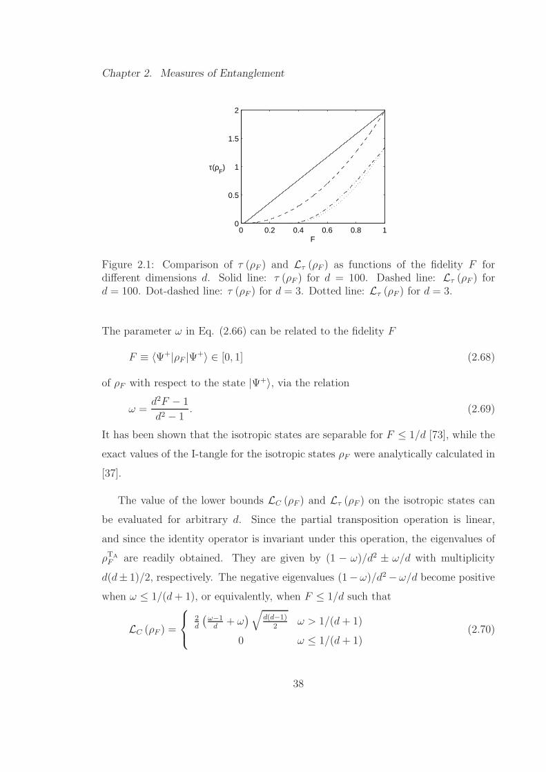
Figure 2.1: Comparison of τ (ρF ) and Lτ (ρF ) as functions of the fidelity F fordifferent dimensions d. Solid line: τ (ρF ) for d = 100. Dashed line: Lτ (ρF ) ford = 100. Dot-dashed line: τ (ρF ) for d = 3. Dotted line: Lτ (ρF ) for d = 3.

The parameter ω in Eq. (2.66) can be related to the fidelity F

F ≡ 〈Ψ+|ρF |Ψ+〉 ∈ [0, 1] (2.68)

of ρF with respect to the state |Ψ+〉, via the relation

ω =d2F − 1

d2 − 1. (2.69)

It has been shown that the isotropic states are separable for F ≤ 1/d [73], while the

exact values of the I-tangle for the isotropic states ρF were analytically calculated in

[37].

The value of the lower bounds LC (ρF ) and Lτ (ρF ) on the isotropic states can

be evaluated for arbitrary d. Since the partial transposition operation is linear,

and since the identity operator is invariant under this operation, the eigenvalues of

ρTAF are readily obtained. They are given by (1 − ω)/d2 ± ω/d with multiplicity

d(d± 1)/2, respectively. The negative eigenvalues (1− ω)/d2 − ω/d become positive

when ω ≤ 1/(d+ 1), or equivalently, when F ≤ 1/d such that

LC (ρF ) =

2d

(ω−1d

+ ω)√d(d−1)

2ω > 1/(d+ 1)

0 ω ≤ 1/(d+ 1)(2.70)

38


The behaviors of the I-tangle τ(ρF ) and of Lτ (ρF ) for the isotropic states are

depicted in Fig. 2.1. For d = 2, the two functions assume the same values, while for

larger dimensions and constant fidelity, the difference between the lower bound and

the I-tangle increases. In the limit d → ∞, τ(ρF ) and Lτ (ρF ) behave as√

2F and

2F 2, respectively. Similarly, the I-concurrence C(ρF ) and LC (ρF ) may be calculated

analytically. Here we find that the two quantities agree over the isotropic states for

any dimension d, demonstrating that the isotropic states saturate our lower bound.

2.3 Summary

The conditions for a function of a quantum state to be a good measure of entangle-

ment are relatively straightforward; it must be non-increasing, on average, under the

set of LOCC protocols and under mixing. Any pure state entanglement monotone

satisfying these criteria may be readily extended to mixed states via the convex-roof

formalism. The evaluation of such functions is, however, computationally intractable

for many cases of interest. Accordingly, there is much interest in identifying quanti-

ties, such as the negativity, that are computable in the most general situations, even

though they may lack a clear resource-based interpretation.

The entanglement measures derived in Section 2.2 comprise classes of monotones

based on the positive partial transpose criterion for separability, and on the connec-

tion between the theory of majorization and comparative disorder. In this larger

context, the negativity is seen to be one specific example of such a function. Other

instances (with appropriate scaling) yield lower bounds on the I-concurrence and the

I-tangle, providing useful tools for investigations of quantum information theoretic

concepts and fundamental quantum mechanics. Apart from offering a larger struc-

ture from which to view these different entanglement measures, each member in this

new family of functions also possesses an analytic form that may be evaluated in the

39


most general situations. In fact, as we will see in the next chapter, our results enable

the quantification of entanglement in the context of a multipartite system of both

theoretical and experimental significance for which there are no known closed-form

solutions for any of the convex roof-based measures.

40

Chapter 3

Entanglement Sharing in the

Tavis-Cummings Model

3.1 Introduction

The development of a mathematically rigorous theory of entanglement is highly de-

sirable for investigating foundational issues in quantum mechanics, as well as for an-

alyzing specific entanglement-enhanced information processing tasks. The previous

chapter makes it clear that, while a consistent method of quantifying entanglement

under the most general circumstances has not yet been formulated, progress has

been made in certain specific cases. In fact, it turns out that the current state of

the theory of entanglement is capable of yielding an essentially complete analysis of

the quantum correlations arising in the two-atom Tavis-Cummings model (TCM), a

system of both theoretical and experimental significance [42]. This chapter presents

a detailed analysis of the different types of entanglement (corresponding to the dif-

ferent possible partitions of the system into subsystems) evolving in the two-atom

TCM as a function of time.

41

Chapter 3. Entanglement Sharing in the Tavis-Cummings Model

This investigation is motivated by the opportunity to employ several different

results from the theory of entanglement in order to study the dynamical evolution

of quantum correlations in a nontrivial, yet experimentally realizable system. One

specific goal of this work is to lay a foundation for future study of the relationship

between the degree of entanglement in a system and the measurement backaction,

or information-disturbance tradeoff [74, 75, 76], that occurs when measuring one

subsystem in order to gain information about a second, correlated subsystem in the

context of the TCM. This is seen as a necessary step toward being able to perform

feedback and control of atomic ensembles with possible applications in the field of

quantum computation.

The control of quantum systems through active measurement and feedback has

been developing at a rapid pace. In a typical scenario, a single atom is monitored

indirectly through its coupling to a traveling probe such as a laser beam. The

scattered beam and the system become correlated, and a subsequent measurement of

the probe leads to backaction on the system. A coherent drive applied to the system

can then be made conditional on the measurement record, leading to a closed-loop

control model [77, 78]. Such a protocol has been implemented to control a single

mode electromagnetic field in a cavity [79], and has been envisioned for controlling a

variety of systems such as the state of a quantum dot in a solid [80], the state of an

atom coupled to a cavity mode [81], and the motion of a micro-mechanical resonator

coupled to a Cooper pair charge box [82].

A common theme in the examples given above is that measurements are made

on single copies of the quantum system of interest. However, in many situations one

does not have access to an individually addressable system. In a gas, for example,

preparing and/or addressing individual atoms is extremely difficult. In situations

such as this, it is useful to think of the entire ensemble as a single many-body system.

Indeed, recent experiments [83, 84] and theoretical proposals [85] have explored the

42


control of such ensembles from the point of view of the Dicke model [86], where a

collection of N two-level atoms is treated as a pseudo-spin with J = N/2.

Measurement backaction on the pseudo-spin can lead to squeezing of the quantum

fluctuations [83, 84, 85], which may be enhanced through active closed-loop control

[77, 78]. This squeezing can reduce the quantum fluctuations of an observable as in,

for example, the reduction of “projection noise” leading to enhanced precision mea-

surements in an atomic clock [87]. Moreover, spin-squeezing is related to quantum

entanglement between the atomic members of the ensemble [88]. This entanglement

arises not through direct interaction between the atoms, but through their coupling

to a common “quantum bus” in the form of an applied probe.

Measures of entanglement associated with these spin-squeezed states have been

studied by Stockton, et. al., [86] under the assumption that all of the atoms in the

ensemble are symmetrically coupled to the bus. However, completely quantifying

multipartite entanglement in the most general cases is extremely difficult, and as yet,

an unsolved problem [53]. Here we consider the simplest possible ensemble consisting

of two two-level atoms. Although at first sight this might appear trivial, when such a

system is coupled to a quantum bus a rich structure emerges. Again, we consider the

simplest realization of the bus – a single mode quantized electromagnetic field. The

resulting physical system then corresponds to the two-atom Tavis-Cummings model

[89]. A thorough understanding of the dynamical evolution of the TCM has obvious

implications for the performance of quantum information processing [2, 90, 91], as

well as for our understanding of fundamental quantum mechanics [2, 92]. Bipartite

entanglement has been investigated in this system for the one-atom case, known as

the Jaynes-Cummings model, for initial pure states [93] and mixed states [94, 95] of

the field.

The two-atom TCM consists of two two-level atoms, or qubits, coupled to a sin-

gle mode of the electromagnetic field in the dipole and rotating-wave approximations

43


[89]. This model admits a total of five different possible partitionings, each of which

may contain varying degrees of entanglement as a function of time. These five differ-

ent partitions are (a) the bipartite division of the system into a subsystem consisting

of the field and a second subsystem consisting of the ensemble of two atoms, (b)

the bipartite division of the system into a subsystem consisting of a single two-level

atom and a second subsystem containing the remainder, i.e., the remaining atom

and the field, (c) the two atoms treated as separate subsystems, with the field being

traced over, (d) a single atom and the field treated as separate subsystems, with the

remaining atom being traced over, and (e) a single partition containing the entire

tripartite system (capable of supporting irreducible three-body correlations).

Taken as a whole, the two-atom TCM in an overall pure state constitutes a tri-

partite quantum system in a Hilbert space with tensor product structure 2⊗ 2⊗∞.

Entanglement in tripartite systems has been studied by Coffman, et. al., [28] for the

case of three qubits. They found that such quantum correlations cannot be arbi-

trarily distributed amongst the subsystems; the existence of three-body correlations

constrains the distribution of the bipartite entanglement which remains after tracing

over any one of the qubits. For example, in a GHZ-state [38],

|GHZ〉 =1√2(|000〉 + |111〉, (3.1)

tracing over any one qubit results in a maximally mixed state containing no entan-

glement between the remaining two qubits. In contrast, for a W-state,

|W〉 =1√3(|001〉+ |010〉 + |100〉, (3.2)

the average remaining bipartite entanglement is maximal [70]. Coffman, et. al., an-

alyzed this phenomenon of entanglement sharing [28], using the tangle between two

qubits as defined in Eq. (2.23). In order to complete this analysis, they also intro-

duced a quantity known as the residual tangle to quantify the irreducible tripartite

correlations in a three qubit system [28].

44


Here, we extend the analysis of entanglement sharing to the case of the two-atom

TCM [42]. This has implications for the study of quantum control of ensembles. For

example, if we imagine that the quantum bus is measured, e.g., the field leaks out

of the cavity and is then detected, then the degree of correlation between the field

and one of the atoms determines the degree of backaction on one atom. We can then

quantify the degree to which one can perform quantum control on a single member

of an ensemble even when one couples only collectively to the entire ensemble. We

accomplish this by extending the residual tangle formalism of Coffman, et. al., to

our 2 ⊗ 2 ⊗∞ system.

The remainder of this chapter is organized as follows. First, the important fea-

tures of the TCM are reviewed in Section 3.2. Using the formalism introduced in

Section 2.1.3, we then calculate the tangle for each of the bipartite partitions of this

tripartite system in Section 3.3. We will find an approximate analytic expression for

the tangle between the field and the ensemble in the limit of large average photon

number and in the Markoff approximation which provides further insight into these

results. In Section 3.4, we study the irreducible tripartite correlations in the system

using our proposed generalization of the residual tangle. Finally, we summarize our

results and suggest possible directions for further research in Section 3.5.

3.2 The Tavis-Cummings Model

The Tavis-Cummings model (TCM) [89] (or “Dicke model”[96]) describes the sim-

plest fundamental interaction between a single mode of the quantized electromagnetic

field and a collection of N atoms under the two-level and rotating wave approxima-

45


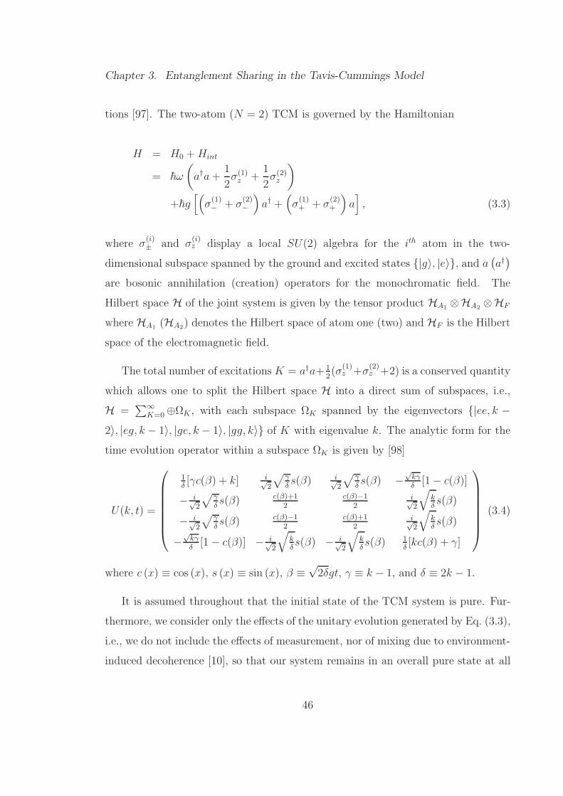
tions [97]. The two-atom (N = 2) TCM is governed by the Hamiltonian

H = H0 +Hint

= ~ω

(a†a+

1

2σ(1)z +

1

2σ(2)z

)

+~g[(σ

(1)− + σ

(2)−

)a† +

(σ

(1)+ + σ

(2)+

)a], (3.3)

where σ(i)± and σ

(i)z display a local SU(2) algebra for the ith atom in the two-

dimensional subspace spanned by the ground and excited states |g〉, |e〉, and a(a†)

are bosonic annihilation (creation) operators for the monochromatic field. The

Hilbert space H of the joint system is given by the tensor product HA1 ⊗HA2 ⊗HF

where HA1 (HA2) denotes the Hilbert space of atom one (two) and HF is the Hilbert

space of the electromagnetic field.

The total number of excitations K = a†a+ 12(σ

(1)z +σ

(2)z +2) is a conserved quantity

which allows one to split the Hilbert space H into a direct sum of subspaces, i.e.,

H =∑∞

K=0 ⊕ΩK , with each subspace ΩK spanned by the eigenvectors |ee, k −2〉, |eg, k − 1〉, |ge, k − 1〉, |gg, k〉 of K with eigenvalue k. The analytic form for the

time evolution operator within a subspace ΩK is given by [98]

U(k, t) =

1δ[γc(β) + k] i√

2

√γδs(β) i√

2

√γδs(β) −

√kγδ

[1 − c(β)]

− i√2

√γδs(β) c(β)+1

2c(β)−1

2i√2

√kδs(β)

− i√2

√γδs(β) c(β)−1

2c(β)+1

2i√2

√kδs(β)

−√kγδ

[1 − c(β)] − i√2

√kδs(β) − i√

2

√kδs(β) 1

δ[kc(β) + γ]

(3.4)

where c (x) ≡ cos (x), s (x) ≡ sin (x), β ≡√

2δgt, γ ≡ k − 1, and δ ≡ 2k − 1.

It is assumed throughout that the initial state of the TCM system is pure. Fur-

thermore, we consider only the effects of the unitary evolution generated by Eq. (3.3),

i.e., we do not include the effects of measurement, nor of mixing due to environment-

induced decoherence [10], so that our system remains in an overall pure state at all

46


times. Finally, by assuming an identical coupling constant g between each of the

atoms and the field, the Hamiltonian is symmetric under atom-exchange. This in-

variance under the permutation group was used by Stockton, et. al., [86] to analyze

the entanglement properties of very large ensembles. We will also make use of this

fact in order to reduce the number of different partitioning schemes that one needs

to consider when studying entanglement sharing in the two-atom TCM.

3.3 Bipartite Tangles in the Two-Atom TCM

Let the two atoms in the ensemble be denoted by A1 and A2, respectively, and the

field, or quantum bus, by F . Because of the assumed exchange symmetry, there are

four nonequivalent partitions of the two-atom TCM into tensor products of bipartite

subsystems: (i) the field times the two-atom ensemble, F ⊗ (A1A2), (ii) one atom

times the remaining atom and the field, A1⊗(A2F ) ≡ A2⊗(A1F ), (iii) the two atoms

taken separately, having traced over the field, A1 ⊗ A2, and (iv) one of the atoms

times the field, having traced over the other atom, A1 ⊗ F ≡ A2 ⊗ F . We calculate

how the tangle for each of these partitions evolves as a function of time under TCM

Hamiltonian evolution using the formalism reviewed in Section 3.2. Taking the initial

state to be a pure product state of the field with the atoms, we capture the key

features of the tangle evolution by considering three classes of initial state vectors,

|e〉A1⊗ |e〉A2

⊗ |n〉F ≡ |ee, n〉 , (3.5a)

|ee, α〉 or |gg, α〉 , (3.5b)

and

1√2

(|eg〉 + |ge〉) ⊗ |α〉 or1√2

(|gg〉 + |ee〉) ⊗ |α〉 , (3.5c)

where |g(e)〉 denotes the ground (excited) state of the atom, |n〉 denotes a Fock state

field with n photons, and |α〉 denotes a coherent state field with an average number

47


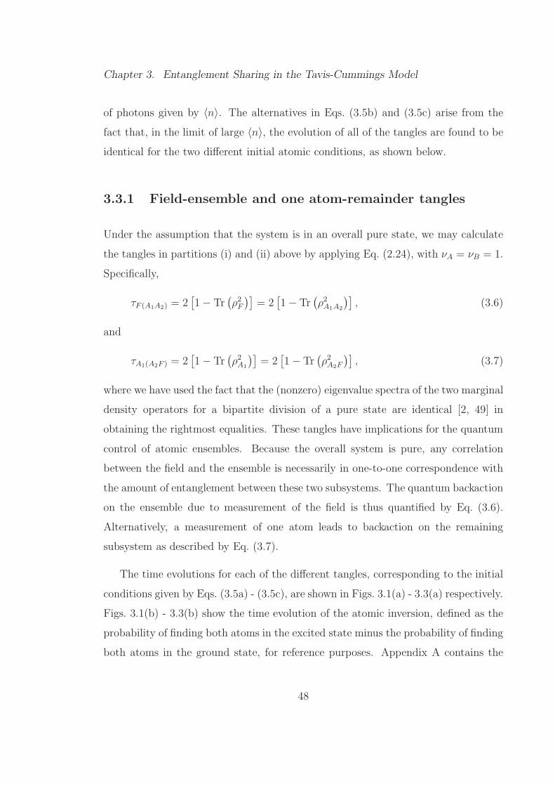
of photons given by 〈n〉. The alternatives in Eqs. (3.5b) and (3.5c) arise from the

fact that, in the limit of large 〈n〉, the evolution of all of the tangles are found to be

identical for the two different initial atomic conditions, as shown below.

3.3.1 Field-ensemble and one atom-remainder tangles

Under the assumption that the system is in an overall pure state, we may calculate

the tangles in partitions (i) and (ii) above by applying Eq. (2.24), with νA = νB = 1.

Specifically,

τF (A1A2) = 2[1 − Tr

(ρ2F

)]= 2

[1 − Tr

(ρ2A1A2

)], (3.6)

and

τA1(A2F ) = 2[1 − Tr

(ρ2A1

)]= 2

[1 − Tr

(ρ2A2F

)], (3.7)

where we have used the fact that the (nonzero) eigenvalue spectra of the two marginal

density operators for a bipartite division of a pure state are identical [2, 49] in

obtaining the rightmost equalities. These tangles have implications for the quantum

control of atomic ensembles. Because the overall system is pure, any correlation

between the field and the ensemble is necessarily in one-to-one correspondence with

the amount of entanglement between these two subsystems. The quantum backaction

on the ensemble due to measurement of the field is thus quantified by Eq. (3.6).

Alternatively, a measurement of one atom leads to backaction on the remaining

subsystem as described by Eq. (3.7).

The time evolutions for each of the different tangles, corresponding to the initial

conditions given by Eqs. (3.5a) - (3.5c), are shown in Figs. 3.1(a) - 3.3(a) respectively.

Figs. 3.1(b) - 3.3(b) show the time evolution of the atomic inversion, defined as the

probability of finding both atoms in the excited state minus the probability of finding

both atoms in the ground state, for reference purposes. Appendix A contains the

48


0 0.2 0.4 0.6 0.8 1 1.2 1.4 1.6 1.8 2

0

0.2

0.4

0.6

0.8

1

1.2

1.4(a)

gt

Tan

gles

0 0.2 0.4 0.6 0.8 1 1.2 1.4 1.6 1.8 2−1

−0.8

−0.6

−0.4

−0.2

0

0.2

0.4

0.6

0.8

1(b)

gt

Ato

mic

Inve

rsio

nFigure 3.1: TCM evolution for both atoms initially in the excited state and the fieldin an initial Fock state with n = 10. (a) Solid curve (red): Field-ensemble tangleτF (A1A2); Large-dotted curve (green): One atom-remainder tangle τA1(A2F ); Dashedcurve (black): Atom-atom tangle τA1A2 . (Note that the atom-atom tangle is alwayszero for the given initial condition.); Dot-dashed curve (pink): Single atom-fieldtangle τA1F ; Dotted curve (blue): Residual tangle τA1A2F . (b) Atomic inversion ofthe ensemble.

Mathematica code used to numerically evaluate the evolution of all of the different

quantities shown in these figures.

We find, under certain conditions, that the two stretched states in Eq. (3.5b) lead

to identical evolution for the tangles in all of the bipartite partitions of the system,

corresponding to the curves shown in Fig. 3.2(a). Similarly, the two symmetric

states given in Eq. (3.5c) both yield the curves shown in Fig. 3.3(a). This behavior

can be derived under a set of highly accurate approximations. In the limit of large

average photon number, an initial coherent state field with zero phase will remain

approximately separable from the atomic ensemble in an eigenstate of Jx ≡ J+ + J−

up to times on the order of 〈n〉 /g where, in the pseudospin picture, J± ≡ σ(1)± +σ

(2)± .

This follows immediately from the time evolution operator generated by Hint in

Eq. (3.3) in the interaction picture. The key observation is that, for a macroscopic

49


0 10 20 30 40 50 60 70 80 90 100−0.2

0

0.2

0.4

0.6

0.8

1

1.2

1.4(a)

gt

Tan

gles

Field−EnsembleOne Atom−RestAtom−AtomOne Atom−FieldI−Residual Tangle

0 10 20 30 40 50 60 70 80 90 100−1

−0.8

−0.6

−0.4

−0.2

0

0.2

0.4

0.6

0.8(b)

gt

Ato

mic

Inve

rsio

nFigure 3.2: TCM evolution for both atoms initially in a stretched state and the fieldin an initial coherent state with 〈n〉 = 100. (a) Solid curve (red): Field-ensembletangle τF (A1A2); Large-dotted curve (green): One atom-remainder tangle τA1(A2F );Dashed curve (black): Atom-atom tangle τA1A2 ; Dot-dashed curve (pink): Singleatom-field tangle τA1F ; Dotted curve (blue): I-Residual tangle τA1A2F . (b) Atomicinversion of the ensemble.

field, the removal or addition of a single photon has a negligible effect. This allows

one to approximate the time evolution operator by exp−iHintt/~ ≈ exp−ig√

〈n〉Jxt.

Thus, the eigenstates of Jx form a convenient basis to use in describing the state

of the atomic ensemble. This approach was taken by Gea-Banacloche in analyzing

the behavior of the single atom Jaynes-Cummings model [99] and the generation

of macroscopic superposition states [100], and extended to the multi-atom TCM by

Chumakov, et. al., [101, 102, 103].

We take as the appropriate basis the three symmetric eigenstates of Jx, which we

label by m = -1, 0, and 1; the singlet state, J = 0, is a dark state and thus does not

couple to the field. Writing the initial state of the system as

|ψ(0)〉 =

1∑

m=−1

dm |m〉 ⊗ |α〉 , (3.8)

and using the factorization approximation [101], we find that the state of the system

50


0 10 20 30 40 50 60 70 80 90 100−0.2

0

0.2

0.4

0.6

0.8

1

1.2(a)

gt

Tan

gles

Field−EnsembleOne Atom−RestAtom−AtomOne Atom−FieldI−Residual Tangle

0 10 20 30 40 50 60 70 80 90 100−0.06

−0.04

−0.02

0

0.02

0.04

0.06(b)

gt

Ato

mic

Inve

rsio

nFigure 3.3: TCM evolution for the atoms initially in a symmetric state and the fieldin an initial coherent state with 〈n〉 = 100. (a) Solid curve (red): Field-ensembletangle τF (A1A2); Large-dotted curve (green): One atom-remainder tangle τA1(A2F );Dashed curve (black): Atom-atom tangle τA1A2 ; Dot-dashed curve (pink): Singleatom-field tangle τA1F ; Dotted curve (blue): I-Residual tangle τA1A2F . (b) Atomicinversion of the ensemble.

up to times on the order of 〈n〉 /g is given by

|ψ(t)〉 ≈1∑

m=−1

dm |Am(t)〉 ⊗ |φm(t)〉 , (3.9)

where |Am(t)〉 and |φm(t)〉 are the time-evolved atomic and field states, respectively.

The marginal density operator for the two atoms is then

ρA1A2(t) ≈∑

l,m

d∗l dm |Am(t)〉〈Al(t)| fml (gt, 〈n〉) , (3.10)

where fml (gt, 〈n〉) ≡∑

n 〈n | φm(t)〉〈φl(t) | n〉. We find that this function has “mem-

ory” only for t ≪√

〈n〉/g, and behaves very much like a delta function for longer

time scales. Effectively, the large dimensional Hilbert space of the field acts as

a broadband reservoir for the atoms – the generalization of the familiar “collapse”

phenomenon in the Jaynes-Cummings model. This “Markoff” approximation is valid

up to times on the order of 2π√〈n〉/g, corresponding to the well-known revival time

51


in the Jaynes-Cummings Model [99]. Making this approximation in Eq. (3.10), the

states |Am (t)〉 act effectively as a “pointer basis” for decoherence [10] of the atomic

density matrix, i.e.,

ρA1A2(t) ≈∑

m

|dm|2 |Am(t)〉〈Am(t)| . (3.11)

Substituting this formula into Eq. (3.6) yields

τF (A1A2)(t) ≈ 2

1 − 1

4[c− h(t′)]

, (3.12)

where

c ≡ 4(|d−1|4 + |d0|4 + |d1|4

)+ 2 |d0|2 |d1|2

+ |d−1|2(2 |d0|2 + 3 |d1|2

)− 4 |d−1|2 |d1|2 (3.13)

h (t′) ≡ 2 |d0|2(|d−1|2 + |d1|2

)cos (4t′) + |d−1|2 |d1|2 cos (8t′) , (3.14)

and

t′ ≡ gt

2√〈n〉 − N

2+ 1

2

. (3.15)

Under the factorization and Markoff approximations, the field-ensemble tangle

is given by a constant term c that depends only on the initial probabilities to find

the atomic ensemble in each of the Jx eigenstates, and a time-dependent piece h(t′).

These probabilities depend solely on the absolute squares of the expansion coefficients

of the atomic state given by Eq. (3.8). It is now clear why certain initial atomic

conditions result in identical evolution for the different tangles. For example, the

atomic states |gg〉 and |ee〉 both satisfy

|d−1| = |d1| =1

2and |d0| =

1√2, (3.16)

52


0 10 20 30 40 50 60 70 80 90 1000

0.2

0.4

0.6

0.8

1

1.2

1.4

gt

Tan

gle

Figure 3.4: Exact field-ensemble tangle: Solid (red) curve, and approximate formula:Dashed (black) curve for an initial stretched atomic state and coherent state fieldwith 〈n〉 = 500.

corresponding to identical evolution for all of the tangles shown in Fig. 3.2(a). Sim-

ilarly, the atomic states 1/√

2 (|eg〉 + |ge〉) and 1/√

2 (|ee〉 + |gg〉) both satisfy

|d−1| = |d1| =1√2

and |d0| = 0, (3.17)

corresponding to the curves shown in Fig. 3.3(a). More generally, this property

holds for any class of initial states∣∣ψ(i) (0)

⟩having the form of Eq. (3.8) such that∣∣∣d(i)

m

∣∣∣ =∣∣∣d(j)m

∣∣∣, m ∈ −1, 0, 1. One immediate consequence of this result is that

the relative phase information encoded in the initial state of the atomic system is

irrelevant to the evolution of the field-ensemble tangle.

The field-ensemble tangle calculated according to Eq. (3.6) and the approximation

given by Eq. (3.12) for an initial stretched atomic state and an initial coherent state

field with 〈n〉 = 500 are shown by the solid (red) and dashed (black) curves in Fig. 3.4,

respectively. The approximation is seen to track the exact evolution extremely well

over the range of its validity. The discrepancy at very small times is explained by

the fact that at these times the Markoff approximation breaks down. It is also seen

53


that our approximate solution does not capture the small dip in the field-ensemble

tangle occurring at t = π√〈n〉/g. The absence of this feature can be explained

by noting that in making the Markoff approximation we have effectively wiped out

any information regarding the initial coherence between the |m = −1〉 and |m = 1〉states. The presence of this dip is then seen to be dependent upon the existence of

this coherence. This is borne out by the fact that the dip in the field-ensemble tangle

in Fig. 3.2(a) is much shallower than that in Fig. 3.3(a), where the initial atomic

expansion coefficients are given by Eqs. (3.16) and (3.17), respectively.

3.3.2 Atom-atom tangle

Given an initial state, we time-evolve the system according to the dynamics governed

by Eq. (3.3), and then trace over the field subsystem. The tangle of the two-atom

mixed state ρA1A2 (t) may then be calculated according to Eq. (2.23). The resulting

atom-atom tangles corresponding to the initial conditions in Eqs. (3.5a) - (3.5c) are

depicted by the dashed (black) curves in Figs. 3.1(a) - 3.3(a), respectively. These

curves yield direct insight into the state of the atomic ensemble as a function of

time. Specifically, the atom-atom tangle quantifies the degree to which the ensemble

behaves as a collective entity, rather than as two individual particles.

It is somewhat surprising that for the initial condition given by Eq. (3.5a), i.e.,

when the field is initially in a Fock state with any value for n, the atom-atom tangle

remains zero at all times, whereas the evolution of the atom-atom tangle resulting

from an initial coherent state field is nontrivial and, in general, nonzero. In order to

better understand these observations, we have performed a preliminary investigation

into the evolution of the atom-atom tangle for initial conditions other than those

given by Eqs. (3.5a) - (3.5c). When the field is initially in a Fock state and both

atoms start in the ground state, the loss of an excitation in the field can result in the

54


creation of an excitation in the atomic ensemble. This produces entanglement be-

tween the field and the ensemble and in the single atom-field and one atom-remainder

partitions. Since it is not possible to distinguish in which atom the excitation is cre-

ated, the two atoms become entangled with each other as well. It is found that the

atom-atom entanglement falls off as 1/n2 so that, in the limit of a highly excited Fock

state, these initial conditions yield results reminiscent of those found in Fig. 3.1(a).

Specifically, we find that the entanglement in all of the different subsystem partitions

always oscillate in phase at twice the Rabi frequency, and that the atom-atom tangle

approaches zero as n becomes large.

Next, we considered the case when both atoms initially reside in a stretched state,

and the initial field state consists of a coherent superposition of two neighboring

Fock states. We find, on a time scale much longer than that given by the inverse of

the associated Rabi frequencies, that the overall behavior again closely resembles the

evolution seen for an initial field consisting of a single Fock state. Specifically, we find

that the general features of all of the different bipartite tangles oscillate in phase with

one another. However, on much shorter time-scales, the effects of dephasing between

the two Rabi frequencies become apparent, yielding the first clues regarding how the

observed coherent state behavior arises in terms of initial Fock state superpositions.

At the revival time, when there is a partial rephasing of the Rabi frequencies, all

of the bipartite tangles decrease simultaneously, while at other times the tangles

in certain bipartite partitions may be completely out of phase with one another.

It seems likely that a detailed investigation of these initial findings will provide a

quantitative explanation for the large scale Fock-like behavior seen in Fig. 3.2.

55


3.3.3 Single atom-field tangle

The final bipartite partition of the two-atom TCM is that consisting of a single

atom, say A1, as one subsystem and the field F as the second subsystem. Again by

exchange symmetry τA1F = τA2F , so we need calculate only one of these quantities.

Because the tripartite system is in an overall pure state, the Schmidt decomposition

theorem [2, 49] implies that the marginal density operator ρA1F has at most rank

two. The rank of the reduced density matrix is set by the dimension of the smallest

subsystem, which in this case is a two-level atom. This is exactly the scenario

envisioned by Osborne [59], as described in Section 2.1.3. The tangle corresponding

to this partition, A1⊗F , is computed by first tracing over the state of the remaining

atom, A2, and then applying Eq. (2.26). Employing this procedure,

τA1F = Tr (ρA1F ρA1F ) + 2λ(A1F )min

[1 − Tr

(ρ2A1F

)], (3.18)

where λ(A1F )min represents the minimum eigenvalue of the Osborne M matrix [59] gen-

erated from the marginal density operator ρA1F . The dot-dashed (pink) curves in

Figs. 3.1(a) - 3.3(a) give the time evolution of the single atom-field tangle for the

different initial conditions considered.

We are now in possession of closed forms for the tangles of all bipartite parti-

tions of the two-atom TCM. Any other entanglement that the system may possess

must necessarily be in the form of irreducible three-body quantum correlations. In

Section 3.4 we review the residual tangle formalism introduced by Coffman, et. al.,

in order to quantify this type of tripartite entanglement in a system of three qubits.

We then propose a generalization of this quantity that is applicable to a 2 ⊗ 2 ⊗D

system in an overall pure state. This extension of the tangle formalism allows us to

study the phenomenon of entanglement sharing in the two-atom TCM.

56


3.4 Entanglement Sharing and the Residual

Tangle

Coffman, et. al., analyze the phenomenon of entanglement sharing for a system of

three qubits A, B, and C in an overall pure state in full generality by introducing

a quantity known as the residual tangle [28]. This definition is motivated by the

observation that the tangle of A with B plus the tangle of A with C cannot exceed

the tangle of A with the joint subsystem BC, i.e.,

τAB + τAC ≤ τA(BC). (3.19)

Here, τAB and τAC are calculated according to Eq. (2.23), and τA(BC) may be obtained

from Eq. (2.24) with νA = νB = 1.

The original proof [28] of the inequality in Eq. (3.19), which forms the heart

of the phenomenon of entanglement sharing for the case of three qubits, may be

substantially simplified by making use of certain results due to Rungta, et. al.

Specifically, we note that [58]

Tr (ρxyρxy) = 1 − Tr(ρ2x

)− Tr

(ρ2y

)+ Tr

(ρ2xy

)≥ 0 (3.20)

for subsystems x and y having arbitrary Hilbert space dimensions. Under the as-

sumption that x and y are in an overall pure state with a third subsystem z, Eq.

(3.20) may be rewritten

Tr (ρxyρxy) = 1 − Tr(ρ2x

)− Tr

(ρ2y

)+ Tr

(ρ2z

)≥ 0, (3.21)

where we have used the equality of the nonzero eigenvalue spectra of ρxy and ρz.

Then, by the observation [28] that for an arbitrary state of two qubits A and B, the

following upper bound on the tangle defined by Eq. (2.23) holds

τ2 (ρAB) ≤ Tr (ρAB ρAB) , (3.22)

57


and by Eq. (2.24) with νA = νB = 1, the inequality in Eq. (3.19) follows immediately.

Subtracting the terms on the left hand side of Eq. (3.19) from that on the right

hand side yields a positive quantity referred to as the residual tangle

τABC ≡ τA(BC) − τAB − τAC . (3.23)

The residual tangle is interpreted as quantifying the inherent tripartite entanglement

present in a system of three qubits, i.e., the entanglement that cannot be accounted

for in terms of the various bipartite tangles. This interpretation is given further

support by the observation that the residual tangle is invariant under all possible

permutations of the subsystem labels [28].

We wish to generalize the residual tangle, defined for a system of three qubits, to

apply to a 2⊗ 2⊗D quantum system in an overall pure state so that we may study

entanglement sharing in the two-atom TCM. Note that we already have all of the

other tools needed for such an analysis. Specifically, from Section 3.3, we know the

analytic forms for all of the different possible bipartite tangles in such a system.

Any proper generalization of the residual tangle must, at a minimum, be a positive

quantity, and be equal to zero if and only if there is no tripartite entanglement in the

system, i.e., if and only if all of the quantum correlations can be accounted for using

only bipartite tangles. It should also reduce to the definition of the residual tangle

in the case of three qubits. Further it is reasonable to require, if this is to be a true

measure of irreducible three-body correlations, that symmetry under permutation

of the subsystems be preserved, and that it remain invariant under local unitary

operations. Finally, we conjecture that this quantity satisfies the requirements (2.2)

and (2.3) for being an entanglement monotone [104, 36] under the set of stochastic

local operations and classical communication (SLOCCs), or equivalently, under the

set of invertible local operations [70]. We limit the monotonicity requirement to this

restricted set of operations since, in the context of entanglement sharing, we are

58


only concerned with LOCCs that preserve the local ranks of the marginal density

operators such that all subsystem dimensions remain constant.

Let A and B again be qubits, and let C now be a D-dimensional system with

the composite system ABC in an overall pure state. We note that, under these

assumptions, we are still capable of evaluating each of the terms on the right hand

side of Eq. (3.23) analytically using the results of Section 3.3. However, we cannot

simply use the definition of the residual tangle (with C now understood to represent a

D-dimensional system) as the proper generalization for two reasons. First, since the

three subsystems are no longer of equal dimension, symmetry under permutations

of the subsystems is lost. However, as we will see, this problem is easily fixed by

explicitly enforcing the desired symmetry. The second, and more difficult problem

to overcome is the fact that the inequality given by Eq. (3.19) no longer holds for

our generalized system because λmin in Eq. (2.26) can be negative, implying that

Eq. (3.23) can also be negative.

The required permutation symmetry may be restored by taking our generalization

of the residual tangle, dubbed the I-residual tangle [42] in reference to previous work,

to be

τABC ≡ 1

3

[τA(BC) + τB(AC) + τC(AB) − 2 (τAB + τAC + τBC)

]. (3.24)

The definition in Eq. (3.24) is obtained by averaging over all possible relabelings of

the subsystems in Eq. (3.23). By inspection, it is obvious that Eq. (3.24) preserves

permutation symmetry. However, it still suffers from the problem that its value can

be negative. In order to deal with this difficulty, we make use of the arbitrary scale

factors appearing in Eqs. (2.24) and (2.25).

Let d be the smaller of the two ‘dimensions’ of two arbitrary dimensional subsys-

tems x and y, i.e., d ≡ min Dx, Dy. Note that by dimension we do not necessarily

mean the total Hilbert space dimension of the physical system under consideration,

59


but only the number of different Hilbert space dimensions that contribute to the for-

mation of the overall pure state of the system. This is a subtle but important point

which automatically enforces insights like those due to Rungta, et. al., [58] and Ver-

straete, et. al., [105] which state that the scale chosen for a measure of entanglement

must be invariant under the addition of extra, but unused, Hilbert space dimensions.

The two-atom TCM provides one example of the relevant physics underlying these

ideas.

Consider, for example, the bipartite partitioning of the TCM into a field sub-

system with DF = ∞, and an ensemble subsystem consisting of the two qubits

with DA1A2 = 4. Any entangled state of the overall system has a Schmidt decom-

position with at most four terms, implying that the field effectively behaves like a

four-dimensional system. Further, since the Tavis-Cummings Hamiltonian given by

Eq. (3.3) does not induce couplings between the field and the singlet state of the

atomic ensemble, i.e., the singlet state is a dark state, the field behaves effectively as

a three-level system, or qutrit, in the context of the TCM. Accordingly, in any entan-

gled state of the field with the ensemble, the field is considered to have a dimension

no greater than three. We employ this revised definition of dimension throughout

the remainder of the paper.

We now make the choice

νAνB =d

2, (3.25)

when calculating each of the bipartite tangles appearing on the right hand side of

Eq. (3.24). This choice is made for several reasons. First of all, it is in complete

agreement with the two qubit case, yielding νAνB = 1 as required. Indeed, when

A, B, and C are all qubits, the residual tangle given by Eq. (3.23) is recovered.

Secondly, it takes differences in the Hilbert space dimensions of the subsystems into

account when setting the relevant scale for each tangle. This is important since, in

order to study the phenomenon of entanglement sharing, the tangles for each of the

60


different bipartite partitions must be compared on a common scale. It is reasonable

that this scale be a function of the smaller of the two subsystem dimensions since,

for an overall pure state, it is this quantity that limits the number of terms in the

Schmidt decomposition. Finally, it is conjectured that a proper rescaling of the

various tangles will result in the positivity of Eq. (3.24).

Note that when applying the proposed rescaling to the terms on the right hand

side of Eq. (3.24), the only term affected is τC(AB), which is rescaled by one-half of

the smaller of the two subsystem dimensions DC and DAB. Each of the other terms

remains unaltered since, in each case, at least one of the two subsystems involved

is a qubit. The net effect of this rescaling is to increase the ‘weight’ of the tangle

between C and AB relative to that of the rest of the tangles. This is reasonable

when one recognizes that both AB, a system of two qubits, and C, a D-dimensional

system (in the case D > 2), have entanglement capacities [29] exceeding that of a

single qubit.

The requirement that the I-residual tangle be invariant under local unitary oper-

ations follows trivially, since each term on the right hand side of Eq. (3.24) is known

to satisfy this property individually. It is still an open question as to whether or

not the proposed rescaling is sufficient to preserve positivity when generalizing the

residual tangle, Eq. (3.23), to the I-residual tangle, Eq. (3.24). However, numerical

calculations give strong evidence that this is the case. The I-residual tangle has been

calculated for over two-hundred million randomly generated pure states of a 2⊗2⊗3

system and of a 2 ⊗ 2 ⊗ 4 system, the only nontrivial possibilities. In each instance

the resulting quantity has been positive. We conjecture that the I-residual tangle

satisfies the requirements of positivity and monotonicity under SLOCC not only for

a 2 ⊗ 2 ⊗ D system, where closed forms currently exist for all of the terms on the

right hand side of Eq. (3.24), but for the most general DA ⊗DB ⊗DC dimensional

tripartite system in an overall pure state (with the proper scaling of each term again

61


given by Eq. (3.25)). The I-residual tangle arising in the context of the two-atom

TCM is shown by the blue curves in Figs. 3.1(a) - 3.3(a).

The residual tangle, as well as our proposed generalization of this quantity, may be

interpreted as a measure of the irreducible tripartite entanglement in a system since

it cannot be accounted for in terms of any combination of bipartite entanglement

measures [28]. A slightly different, and possibly more enlightening interpretation

is that the I-residual tangle quantifies the amount of freedom that a system has in

satisfying the constraints imposed by the phenomenon of entanglement sharing. If the

I-residual tangle of a tripartite system is zero, then each bipartite tangle is uniquely

determined by the values of all of the other bipartite tangles. Alternatively, if τABC

is strictly greater than zero, then the bipartite tangles enjoy a certain latitude in the

values that each may assume while still satisfying the positivity criterion. The larger

the value of the I-residual tangle, the more freedom the system has in satisfying the

entanglement sharing constraints. This reasoning highlights the relationship between

entanglement sharing and the I-residual tangle.

Finally, we may interpret the I-residual tangle as the average fragility of a tri-

partite state under the loss of a single subsystem. That is, if one of the three

subsystems is selected at random and discarded (or traced over), then the I-residual

tangle quantifies the amount of three-body entanglement that is lost, on average. It

is the existence of physically meaningful interpretations such as these which prompt

us to postulate this new measure of tripartite entanglement for a 2 ⊗ 2 ⊗D system

in an overall pure state, rather than to rely on previously defined measures based on

normal forms [105] or on the method of hyperdeterminants [106], for example. At

this point it is unclear what, if any connection these entanglement monotones have

to the entanglement that exists in different bipartite partitions of the system, a key

ingredient in any discussion of entanglement sharing.

The constraint imposed by entanglement sharing on the values of the various

62


bipartite tangles, each of which is known to be a positive function, is simply that

Eq. (3.24) cannot be negative. It then follows that the strongest constraint of this

form is placed on the two-atom TCM when the I-residual tangle is equal to zero. This

occurs (to a good approximation) periodically in Fig. 3.1(a) for the initial condition

given by Eq. (3.5a). It is at these points that each bipartite tangle is uniquely

determined in terms of the values of all of the other bipartite tangles. Conversely,

at one half of this period when the I-residual tangle achieves its maximum value,

the various bipartite partitions enjoy their greatest freedom with respect to how

entanglement may be distributed throughout the system while still satisfying the

entanglement sharing constraints. The distribution of correlations is, of course, still

determined by the initial state of the system and by the TCM time evolution, both

of which we consider to be separate constraints.

Similarly, the dotted (blue) curves in Figs. 3.2(a) and 3.3(a) show the evolution of

the residual tangle for the initial states given by Eqs. (3.5b) and (3.5c), respectively.

Note how the more complicated behavior resulting from an initial coherent state field

arises from a specific superposition of Fock states, the tangles of which all have a

simple oscillatory evolution. This suggests that the phenomenon of entanglement

sharing may offer a useful perspective from which to investigate the way in which

the coherent state evolution results from a superposition of Fock state evolutions.

The fact that the TCM Hamiltonian leads to a nonzero I-residual tangle is inter-

esting in its own right. Inspection of Eq. (3.3) shows that this model does not include

a physical mechanism, e.g., a dipole-dipole coupling term enabling direct interaction

between the two atoms in the ensemble, but only for coupling between the field and

the atoms. Consequently, all interactions between the atoms are mediated by the

electromagnetic field via the exchange of photons, and are in some sense indirect.

This, however, turns out to be sufficient to allow genuine tripartite correlations to

develop in the system as evidenced by values of the I-residual tangle that are strictly

63


greater than zero.

3.5 Summary and Future Directions

The two-atom Tavis-Cummings model provides the simplest example of a collection

of two-level atoms, or qubits, sharing a common coupling to the electromagnetic

field. A detailed understanding of the evolution of entanglement in different bipartite

partitions of this model is valuable for both fundamental theoretical investigations,

and for accurately describing the behavior of certain nontrivial, yet experimentally

realizable systems. Our proposed generalization of the residual tangle augments the

current formalism, and enables one to analyze the irreducible three-body correlations

that arise in a broader class of tripartite systems, providing a tool useful for studying

the phenomenon of entanglement sharing in the context of a physically relevant and

accessible system.

One possible extension of this work would be to generalize this analysis to include

ensembles with an arbitrary number of atoms. This would entail further extensions

of the tangle formalism in order to quantify both the entanglement in a mixed state

of a bipartite system of arbitrary dimensions with rank greater than two, and the

multipartite entanglement in a system with more than three subsystems. Completely

characterizing multipartite entanglement is a difficult and as yet unsolved problem

[28, 42, 53]. Thus, a comprehensive investigation of the phenomenon of entanglement

sharing in the TCM when N > 2 is not currently feasible. However, using the results

of Section 2.2 one may calculate a lower bound on the I-tangle of a mixed state

of an arbitrary bipartite system that provides valuable information regarding the

distribution of entanglement among the different bipartite partitions of the TCM

when N > 2 [43].

Because it is an entanglement monotone, the quantity Lτ (ρ) given by Eq. (2.64),

64


0 20 40 60 80 1000

0.2

0.4

0.6

0.8

gt

τ(ρaf

)

Figure 3.5: Analytic values of τ (ρAF ) (upper curve) and the corresponding lowerbound Lτ (ρAF ) (lower curve) in the two-atom TCM.

captures all of the qualitative features of the I-tangle. Fig. 3.5, which shows the

I-tangle between a single atom and the field in the two atom TCM, as well as the

corresponding lower bound, demonstrates this agreement. Thus, even though we

may not, in general, be capable of analytically evaluating the I-tangles for certain

bipartite partitions of the TCM when N > 2, we may still capture the qualitative

features of the entanglement arising in these partitions by using Lτ (ρ). Such calcula-

tions provide initial insight into the distribution of entanglement and the constraints

imposed by entanglement sharing in the TCM with an arbitrary number of atoms.

Ultimately, one would hope to connect this analysis to the phenomenon of quan-

tum backaction on individual particles when the whole ensemble is measured. The

tradeoff between the information gained about a system and the disturbance caused

to that system is certainly fundamental to quantum mechanics [74, 75, 76]. However,

the relationship of this tradeoff to multiparticle entanglement is far from clear. Such

an understanding would not only be a crucial step in designing protocols for the

quantum control of ensembles, but would also provide deeper insight into the com-

plementary relationship between correlations and correlated entities that we feel lies

65


at the heart of quantum mechanics [44]. The next chapter places this intuition on

a firm foundation by quantifying a tradeoff between bipartite entangled correlations

and information about individual members of multi-qubit systems.

66

Chapter 4

Quantitative Complementarity

Relations

4.1 Introduction

We now move from a discussion of entanglement and its properties to a discussion of

complementarity which, we will argue, is an even more fundamental concept in quan-

tum mechanics. Quantitative relations are introduced in this chapter which imply

that many of the counterintuitive features of entangled quantum systems including:

(i) the fact that maximal information about a composite quantum system does not

necessarily imply maximal information about the component subsystems and (ii) the

phenomenon of entanglement sharing, can be understood as specific consequences of

complementarity in composite systems. This, in turn, has profound implications for

the philosophical foundations of quantum mechanics.

Complementarity is perhaps the most important phenomenon distinguishing sys-

tems that are inherently quantum mechanical from those that may accurately be

treated classically. Accordingly, a thorough understanding of this concept is of fun-

67

Chapter 4. Quantitative Complementarity Relations

damental importance in determining how to properly interpret quantum mechanics

[1], as well as in studying the potential usefulness of quantum systems for enhancing

specific information processing protocols.

Niels Bohr introduced the term complementarity to refer to the fact that infor-

mation about a quantum object obtained under different experimental arrangements

cannot always be comprehended within a single causal picture [4]. We identify the

classical world with precisely those systems and processes for which it is possible to

unambiguously combine the space-time coordinates of objects with the dynamical

conservation laws that govern their mutual interactions. However, in the more gen-

eral setting of quantum mechanics, complementarity precludes the existence of such

a picture. It was this insight that led Bohr to consider complementarity to be the

natural generalization of the classical concept of causality [4].

An alternative statement of complementarity, which makes no reference to exper-

imental arrangements or measurements, states that a quantum system may possess

properties that are equally real, but mutually exclusive. The wave-particle dual-

ity exhibited by a photon in a double-slit experiment [6] and the tradeoff between

the uncertainties in the position and momentum of a subatomic particle governed

by Heisenberg’s relation [7] are two examples of complementarity in single quan-

tum systems. The study of complementarity in composite systems has a fairly short

history by comparison. Nevertheless important progress has been made, especially

in the context of two-particle interferometers, where complementarity relations be-

tween single and two-particle fringe visibilities [107, 108], between distinguishability

and visibility [109], and between the coherence and predictability [110] in a quantum

eraser [97] are known and have been experimentally verified [111, 112, 113]. Addition-

ally, Jaeger, et al., [114] have recently derived a complementarity relation between

multipartite entanglement and mixedness for specific classes of N -qubit systems.

Jakob and Bergou [115] took a major step forward by deriving a complementarity

68


relation, valid for an arbitrary pure state of two qubits, which accounts for (and in

some cases, generalizes) many of the main results put forward in [107, 108, 109, 110].

They showed that an arbitrary normalized pure state |ψ〉 of a two-qubit system

satisfies the expression [115]

C22 (ψ) + ν2

k + p2k = 1. (4.1)

The first term on the left hand side of Eq. (4.1) is the square of the concurrence given

by Eq. (2.14), an inherently bipartite quantity which was shown to be equivalent to

the two-qubit tangle in Section 2.1.3 .

The remaining two terms on the left hand side of Eq. (4.1) are the squares of single

particle properties associated with qubit k = 1, 2. The first of these properties is

the coherence νk of qubit k, which quantifies, e.g., the fringe visibility in the context

of a two-state system incident on an interferometer. Defining the marginal density

operator ρk ≡ Trj (|ψ〉〈ψ|) for j 6= k, the coherence is given by

ν (ρk) ≡ 2∣∣∣Tr(ρkσ

(k)+

)∣∣∣ , (4.2)

where σ(k)+ is the raising operator acting on qubit k. Similarly, the predictability p

which quantifies the a priori information regarding whether qubit k is in the state

|0〉 or the state |1〉, e.g., whether it is more likely to take the upper or lower path in

an interferometer, is given by

p (ρk) ≡∣∣Tr(ρkσ

(k)z

)∣∣ . (4.3)

Here, σz is a Pauli operator and |0〉 (|1〉) is the plus (minus) one eigenvector of σz.

Jakob and Bergou note that Eq. (4.1) becomes an inequality when applied to a

mixed state of two qubits [115]. Here we generalize their result in two ways: (i) to

apply to an arbitrary pure state of N qubits, and (ii) to apply to an arbitrary state

of two qubits, pure or mixed [44]. These expressions shed light on a wide range of

topics in quantum information theory, including the highly investigated connection

69


between entanglement and mixedness [72, 116, 117, 118, 119, 120] about which it was

recently written that, “even for two qubits, the smallest nontrivial bipartite quantum

system, the relation between entanglement and mixedness remains a fascinating open

question” [120]. Our results lead to a complete characterization of the relationship

between these two quantities in exactly this case.

The remainder of this chapter is as follows. In Section 4.2 we derive our two

generalizations of Eq. (4.1) from a single common insight and interpret the various

quantities involved. One immediate implication of our work is an explicit relation-

ship between the residual tangle and the tangles of the different two-qubit marginals

in a pure state of three qubits. The resulting expression illustrates a tradeoff between

the various single particle properties, the bipartite entanglement, and the inherent

three-body quantum correlations encoded in the tripartite quantum state, effectively

reducing the phenomenon of entanglement sharing to a specific instance of comple-

mentarity in this system.

Next we derive a quantity, which we dub the separable uncertainty, that arises

naturally in the context of our second complementarity relation, and show that it is a

good measure of the uncertainty due to ignorance in a quantum state. The introduc-

tion of this quantity completes the two-qubit picture and enables a comprehensive

analysis of the relationship between entanglement and mixedness in such systems.

The section ends with several examples designed to illustrate the usefulness of our

generalized relations. Finally, we discuss potential applications of our results, as well

as some interpretational issues, in Section 4.3.

70


4.2 Multi-Qubit Complementarity Relations

Our two generalizations of Eq. (4.1) both hinge on the observation (which may be

verified by direct computation) that the expression

M (ρk) =1

2− S2 (ρk) (4.4)

holds for an arbitrary state of a single qubit. Here, M (ρk) ≡ 1 − Tr (ρ2k) is the

marginal mixedness of qubit k, and S2 (ρk) ≡ 1/2 [ν2 (ρk) + p2 (ρk)] is the average

of the squares of the single qubit properties defined by Eqs. (4.2) and (4.3). The

mixedness, or linear entropy of a quantum state [121], varies continuously from zero

for pure states to its maximum value of 1/2 for the completely mixed state. The

quantity S2 (ρk) is found to be invariant under local unitary operations performed

on qubit k, and is therefore taken to be a measure of the single particle proper-

ties encoded in ρk. According to Eq. (4.4) then, the marginal mixedness quantifies

our uncertainty regarding the properties possessed by a single qubit. Further, this

expression leads to the relation

N∑

k=1

[M (ρk) + S2 (ρk)

]=N

2, (4.5)

when summed over an arbitrary system of N qubits, and implies a tradeoff between

the single particle properties in such a system and our uncertainty regarding these

properties.

Consider now the case where the N qubits are in an overall pure state. As we

have already seen, the Schmidt decomposition theorem expressed by Eq. (2.8) implies

that the marginal density operators describing the two subsystems resulting from

a bipartite partitioning of this system have the same nonzero eigenvalue spectra.

In particular, this holds for ρk and ρRk, where ρk is the marginal state of the

kth qubit and ρRk is the marginal state of the N − 1 qubits in the set Rk ≡

71


1, 2, . . . , k − 1, k + 1, . . . , N − 1, N. From Eq. (2.24) with νA = νB = 1 it then

follows that 2M (ρk) = τkRk. Combined with Eq. (4.5), this yields

N∑

k=1

[τkRk + 2S2 (ρk)

]= N. (4.6)

Equation (4.6) shows that a complementary relationship exists between the single

particle properties S2 (ρk) and the bipartite quantum correlations τkRk.

As an interesting application of this expression, consider a pure state of three

qubits. Expressing Eq. (4.6) (in the case N = 3) in terms of the symmetric form of

the residual tangle given by Eq. (3.24) yields the relation

τ123 +2

3

[τ12 + τ13 + τ23 + S2 (ρ1) + S2 (ρ2) + S2 (ρ3)

]= 1. (4.7)

It then follows that the entanglement sharing behavior exhibited by this system, as

described in Section 1.3, is essential for ensuring consistency with Eq. (4.7). This ex-

pression governs the underlying complementarity that exists between the potentially

available information about individual subsystems, the bipartite entanglements in

the marginal two-qubit states, and the irreducible tripartite quantum correlations.

We conjecture that this connection between entanglement sharing and complemen-

tarity is a general feature of composite quantum systems.

The derivation of our second generalization of Eq. (4.1) makes use of Eq. (3.20),

from which it immediately follows that

Tr (ρρ) +M (ρ) = M (ρ1) +M (ρ2) (4.8)

for an arbitrary state ρ of two qubits. The quantity Tr (ρρ) + M (ρ) thus provides

an alternative way of calculating the uncertainty regarding single particle properties

encoded in such states. Substituting Eq. (4.8) into Eq. (4.5) in the case N = 2 yields

Tr (ρρ) +M (ρ) + S2 (ρ1) + S2 (ρ2) = 1. (4.9)

72


The explicit role played by the sum of the first two terms in Eq. (4.9) is best

illustrated by an example. The invariance under local unitary operations of both

Tr (ρρ) and M (ρ) allows us to consider, without loss of generality, density matrices

ρc in the computational basis of the form:

ρc =

ω1 a a e

a∗ ω2 f a

a∗ f ∗ ω3 a

e∗ a∗ a∗ ω4

, (4.10)

where 0 ≤ ωi ≤ 1 and∑

i ωi = 1. Equation (4.10) is obtained by reducing the number

of free parameters in an arbitrary density matrix from fifteen to nine via the six free

parameters in a tensor product of two single-qubit unitary operators. In this repre-

sentation the individual coherences for the two qubits are equal, i.e., ν(ρ

(k)c

)= 4 |a|,

k = 1, 2. Accordingly, Tr (ρρ) = Tr (ρcρc) = 2(|e|2 + |f |2 − 4 |a|2 + ω2ω3 + ω1ω4

),

and M (ρ) = M (ρc) = 1 − 2(|e|2 + |f |2 + 4 |a|2

)−∑4

i=1 ω2i . Some algebra then

yields

Tr (ρρ) +M (ρ) =4∑

i=1

σ2i − 2C14 − 2C23 −

1

2

2∑

k=1

ν2(ρ(k)c

), (4.11)

where σ2i = ωi (1 − ωi) is the variance of ωi in the single trial frequencies that result

from a measurement in the computational basis, Cij = −ωiωj is the similarly defined

covariance between ωi and ωj , and 1/2∑2

k=1 ν2(ρ

(k)c

)is the average of the squared

coherences. The variances measure the spreads or uncertainties associated with the

multinomial distribution ωi, the covariances are directly related to predictability

information that is preserved by the spin-flip operation, and the average squared

coherence quantifies the information encoded in the coherences of the individual

qubits. Thus, Tr (ρρ) +M (ρ) is the total uncertainty in the distribution ωi minus

the available information about properties possessed by the individual subsystems,

in complete agreement with Eq. (4.8). The form of ρ given by Eq. (4.10) makes this

73


relationship readily apparent; however it holds for an arbitrary density operator due

to the invariance of each term in Eq. (4.9) under local unitary operations.

Equation (4.9) also enables us to make a connection with the work of Jaeger, et

al. [114] who showed that the following expression (in our notation) holds for an

arbitrary state of N qubits,

Tr (ρρ) +M (ρ) = I (ρ, ρ) . (4.12)

Here, ρ ≡ σ⊗Ny ρ∗σ⊗N

y is the natural generalization of the spin-flip operation. The

quantity I (ρ, ρ), referred to as the indistinguishability, is defined in terms of the

Hilbert-Schmidt distance DHS (ρ− ρ′) ≡√

12Tr[(ρ− ρ′)2] between two density ma-

trices ρ and ρ′ to be [114]

I (ρ, ρ) ≡ 1 −D2HS (ρ− ρ) . (4.13)

This quantity measures the indistinguishability of the state ρ from the operator

ρ, and thus serves as a measure of the spin-flip symmetry of the state. Further,

Eqs. (4.8) and (4.12) imply that, at least in the two-qubit case, the indistinguisha-

bility also represents the total uncertainty in the quantum state regarding single

particle properties.

Combining Eqs. (4.9) and (4.12) in the case N = 2 yields

I (ρ, ρ) + S2 (ρ1) + S2 (ρ2) = 1, (4.14)

which implies a complementary relationship between information about properties

possessed by the individual qubits and the spin-flip symmetry of the state. Substitut-

ing Eq. (4.13) into Eq. (4.14) then leads to the following relationship between single

particle properties and the Hilbert-Schmidt distance between the density operator

and its spin-flip,

DHS (ρ− ρ) =

√S2 (ρ1) + S2 (ρ2). (4.15)

74


Equation (4.15) suggests a geometric picture in which the root mean square values√S2 (ρk) of the single particle properties act like coordinates in the space of two-

qubit density matrices, and shows that the distance between the quantum state and

its spin-flip is determined solely by these local properties. Hence, our results yield a

method of investigating the abstract space of two-qubit density matrices with simple

Euclidean geometry.

Next, in order to determine the role played by entanglement in Eq. (4.9), we

note that an arbitrary two-qubit density matrix may always be written in its unique

optimal Lewenstein-Sanpera decomposition [122]

ρ = λρs + (1 − λ) |ψe〉〈ψe| , (4.16)

where ρs =∑

i piρ(i)1 ⊗ ρ

(i)2 , (0 ≤ pi ≤ 1,

∑i pi = 1) is a separable density matrix,

|ψe〉 is an entangled pure state, and λ ∈ [0, 1] is maximal. Calculating the quantity

Tr (ρρ) using this representation, one finds that

Tr (ρρ) = Tr(λ2ρsρs

)+2λ (1 − λ)Re

⟨ψe |ρs| ψe

⟩+(1 − λ)2

∣∣∣⟨ψe | ψe

⟩∣∣∣2

. (4.17)

The first term in Eq. (4.17) quantifies that part of ρs which is preserved under the

spin-flip operation, and the second quantifies the (real) part of∣∣∣ψe⟩

that overlaps

with ρs. Hence, neither of these terms involve entanglement. On the other hand, the

last term in Eq. (4.17) is directly related to the quantum correlations in the system

as we now demonstrate.

Written in the form of Eq. (4.16), all of the entanglement in the two-qubit state

ρ is concentrated in the pure state |ψe〉 as quantified by the expression [122]

C (ρ) = (1 − λ)C (ψe) . (4.18)

Recalling the definition of the pure state concurrence given by Eq. (2.14) and that the

squared concurrence is equivalent to the tangle for a system of two qubits, Eq. (4.18)

75


implies that

τ (ρ) = (1 − λ)2∣∣∣⟨ψe | ψe

⟩∣∣∣2

. (4.19)

Thus, the last term in Eq. (4.17) represents the entanglement in the state ρ as

quantified by the mixed state tangle given in Eq. (2.25) with νA = νB = 1.

The two fundamental sources of uncertainty regarding single particle properties

in composite quantum systems are: (i) ignorance of their values, and (ii) partial to

total exclusion of these properties due to the presence of entanglement. Recalling

from Eq. (4.8) that Tr (ρρ) + M (ρ) is a measure of the total uncertainty regarding

single particle properties in the quantum state, Eqs. (4.17) and (4.19) imply that the

quantity

η (ρ) = Tr (ρρ) +M (ρ) − τ (ρ) , (4.20)

0 ≤ η (ρ) ≤ 1, is a good measure of the separable uncertainty, or uncertainty due to

ignorance (rather than to the presence of entanglement), in an arbitrary state of two

qubits. For example, since Tr(ψψ)

= τ (ψ) and M (ψ) = 0, we see from Eq. (4.20)

that η (ψ) = 0, demonstrating that pure states contain no separable uncertainty.

Similarly, η (I/4) = 1 for the completely mixed state, implying that the uncertainty

in this case is maximal, and that this state encodes no information regarding either

single particle properties or bipartite correlations. Finally, consider the maximally

entangled states for fixed marginal mixednesses ρm given by [120]

ρm =

x1 0 0√x1x2

0 0 0 0

0 0 1 − x1 − x2 0√x1x2 0 0 x2

, (4.21)

with 0 ≤ x1, x2 ≤ 1 and x1 + x2 ≤ 1. We find that in this case η (ρm) = M (ρm), i.e.,

the separable uncertainty is simply equal to the mixedness.

76


Equation (4.20) completely characterizes the highly investigated connection be-

tween entanglement and mixedness in two-qubit systems by relating these quantities

to the separable uncertainty and spin-flip invariance encoded in ρ. Likewise, com-

bining Eqs. (4.8) and (4.20) yields

η (ρ) = M (ρ1) +M (ρ2) − τ (ρ) . (4.22)

This alternative form of η (ρ) quantifies the relationship between entanglement and

the marginal mixednesses of the individual qubits.

Our second generalization of Eq. (4.1) is finally obtained by combining Eqs. (4.9)

and (4.20), yielding

η (ρ) + τ (ρ) + S2 (ρ1) + S2 (ρ2) = 1. (4.23)

This expression shows that an arbitrary state of two qubits exhibits a complemen-

tary relationship between the amounts of separable uncertainty, entanglement, and

information about single particle properties that it encodes. Further, it reduces to

Eq. (4.1) for a pure state |ψ〉, and has the desirable property that each term is

separately invariant under local unitary operations.

The following examples are adapted from [114] in order to highlight the additional

insights provided by Eq. (4.23) over previous analyses. Consider the set of states for

which I (ρ, ρ) = 0, or equivalently, for which DHS (ρ− ρ) = 1. These states are

maximally distinguishable from their spin-flips. From Eqs. (4.12) and (4.20) we see

that τ (ρ) = M (ρ) = 0 which implies that this class of states is equivalent to the set of

separable pure states. Equation (4.23) confirms that in this case S2 (ρ1)+S2 (ρ2) = 1,

i.e., states of this type possess maximal single particle properties and no bipartite

correlations nor separable uncertainty.

Next, consider the class of states for which M (ρ) = I (ρ, ρ), i.e., for which the

mixedness represents the total uncertainty about single particle properties. Equa-

tions (4.12) and (4.20) then imply that τ (ρ) + η (ρ) = M (ρ), which illustrates the

77


precise relationship between entanglement and mixedness for states of this form.

Further, from Eqs. (4.13) and (4.15) and the fact that the purity P (ρ) = 1−M (ρ),

we surmise that P (ρ) = S2 (ρ1)+S2 (ρ2), yielding an explicit geometric relationship

between the purities and the allowable single particle properties of these states.

As a final example, we consider the states that possess perfect spin-flip symmetry.

These are the states for which ρ = ρ, or by Eq. (4.13) for which I (ρ, ρ) = 1, and

hence, DHS (ρ− ρ) = 0. Equation (4.15) then implies that S2 (ρ1) = S2 (ρ2) = 0,

yielding the result that no state with perfect spin-flip symmetry may encode any

information about single particle properties.

A specific class of states satisfying these conditions are the Werner states ρw [123]

ρw (λ) = λ |Bell〉〈Bell| + 1 − λ

4I2 ⊗ I2, (4.24)

where 0 ≤ λ ≤ 1, |Bell〉 represents one of the four Bell states, and I2 is the identity

operator for a single qubit. The Werner states vary continuously from the completely

mixed state (λ = 0) to a maximally entangled state (λ = 1), and are known to be

separable for λ ≤ 1/3 [63]. It is a simple matter to show that the states given

by Eq. (4.24) satisfy the condition that ρw = ρw. Equation (4.23) then implies

that η (ρw) = 1 − τ (ρw) demonstrating, among other things, that all separable

Werner states are associated with the maximum amount of separable uncertainty,

independent of λ.

Jaeger, et al. claim that Tr (ρρ) is a good measure of multipartite entanglement,

and therefore state that Tr (ρwρw) +M (ρw) = 1 quantifies the relationship between

entanglement and mixedness for the Werner states [114]. However, Tr (ρwρw) fails

to satisfy the requirements for being an entanglement monotone [36], since it does

not assign the same value to all of the separable Werner states. Indeed our results

show that, when considering the class of Werner states the relevant tradeoff occurs

not between entanglement and mixedness, but instead between entanglement and

78


separable uncertainty.

4.3 Discussion and Future Directions

The examples presented above demonstrate that entanglement and separable uncer-

tainty are quite similar in many respects. For instance, both quantities are related

to information in the quantum state (or a lack thereof) which is preserved under

the spin-flip operation. Further, both are invariant under local unitary operations,

implying that they measure properties which are independent of the choice of lo-

cal bases. Finally, Eq. (4.23) shows that both quantities share a complementary

relationship with the properties of the local subsystems as well as with one another.

There are also important differences between entanglement and the separable

uncertainty quantified by η (ρ). First of all, the separable uncertainty vanishes for

all pure states, while entanglement is both a pure and mixed state phenomenon.

Further, as is well known, entanglement cannot be increased on average by local

operations and classical communication (LOCC) [36], while this restriction does not

hold for separable uncertainty where we are always allowed to throw away or ‘forget’

information. Finally, entanglement quantifies the information that we possess regard-

ing the existence of quantum correlations, whereas separable uncertainty quantifies

a lack of information about the individual subsystems.

We conclude from these observations that the entanglement τ (ρ), and the sin-

gle particle properties S2 (ρ1) and S2 (ρ2), are the three fundamental and mutually

complementary attributes of a two-qubit system about which we may possess infor-

mation that does not depend on our choice of local bases. This, in turn, suggests

an interpretation for the tangle as the fiducial measure of uncertainty regarding in-

dividual subsystem properties due to the presence of entanglement, rather than to

our ignorance. Equivalently, because of the relationship between uncertainty and

79


information [26, 16], the tangle also quantifies the amount of information directly

encoded in the quantum correlations of the system.

When dealing with systems composed of more than two subsystems, entangle-

ment sharing becomes possible. Equation (4.7) implies that, at least in the simplest

case of a pure state of three qubits, this phenomenon also has its roots in complemen-

tarity; this time in terms of a tradeoff between the allowed single particle, bipartite,

and tripartite information that such a system may encode. Verifying the conjecture

that entanglement sharing in arbitrary composite systems is generally a consequence

of complementarity requires the extension of relations such as Eq. (4.6) to multi-

partite systems with subsystems of arbitrary dimension. This in turn requires the

identification of the appropriate multipartite generalization of the residual tangle as

well as a determination of which of the possible partitions of such a system contribute

to these relations and how to quantify them.

Because of these difficulties it is, at present, unclear how to further generalize our

results. Fortunately, several potential applications of the complementarity relations

presented here readily suggest themselves. Beyond fully investigating the relation-

ship between entanglement and mixedness made explicit by Eq. (4.20), or, perhaps

more interestingly, between entanglement and the individual subsystem mixednesses

given by Eq. (4.22), our results also seem well-suited to formulating an information

vs. disturbance tradeoff relation (see [76] and references therein) for two-qubit sys-

tems. The complementary behavior exhibited by these systems implies that, loosely

speaking, a certain amount η (ρ) of additional information regarding single particle

properties may be obtained through observation without affecting the entanglement

in the system. However, if one tries to obtain more information than this, then

by Eq. (4.23) the entanglement must decrease. This behavior leads us to conjec-

ture that complementarity between bipartite and single particle properties plays a

fundamental role in the information-disturbance tradeoff phenomenon in composite

80


systems.

A quantitative relation describing the information-disturbance tradeoff in an ar-

bitrary state of two qubits would, e.g., prove useful for incorporating a measurement,

feedback, and control loop into the two-atom Tavis-Cummings model analyzed in the

previous chapter. Eventually, one would hope to generalize the complementarity re-

lation in Eq. (4.23) to apply to arbitrary multipartite systems, and to extract from

this a corresponding information-disturbance tradeoff relation governing these many-

body systems. This would then enable the investigation of feedback and control on

an arbitrarily large ensemble of two-level atoms in the context of the TCM. The

main obstacle to such an extension of the current formalism once again appears to

be the task of quantifying multipartite entanglement.

Finally, our generalized complementarity relations also suggest one possible way

of thinking about the quantum state of a system from an information-theoretic point

of view. Much has been written about the so-called Bayesian interpretation, which

considers the quantum state to be a representation of our subjective knowledge about

a quantum system [25]. One advantage of this interpretation is that the collapse of

the wave function [23] is viewed not as a real physical process, but simply represents a

change in our state of knowledge. However, it is unclear what this knowledge pertains

to since, from this perspective, we are generally prohibited from associating objective

properties with individual systems. This situation becomes even more confusing if

one also contends that a qubit encodes in-principle information i.e. that information

is physical [124], since the Bayesian interpretation fails to make a distinction between

this type of information and the subjective knowledge of an observer. Equations (4.6)

and (4.23) provide some insight regarding these observations, especially in the context

of two-qubit systems.

We first assume, in agreement with the Bayesian interpretation, that the analysis

of any such system must begin with our subjective human knowledge. Accordingly,

81


we assign a quantum state to the system representing this knowledge. Associated

with this quantum state assignment is a value for η (ρ) which quantifies our subjective

uncertainty regarding the in-principle information encoded by the two-qubit system.

In this context Eq. (4.23) implies that, the smaller our separable uncertainty, the

greater our ability to indirectly access and/or manipulate this in-principle informa-

tion via the locally unitarily invariant bipartite correlations τ (ρ) and single particle

properties S2 (ρk), about which we possess subjective information. However, even

when we are able to assign a pure state to the quantum system such that η (ψ) = 0,

Eq. (4.6) substantiates the observation that “maximal information is not complete

and cannot be completed” [25]. This is a direct consequence of the complementary

relationships that exist between (i) the single particle properties ν (ρk) and p (ρk) of

the individual subsystems, and (ii) between the total localized attributes S2 (ρk) of

the subsystems and the inherently bipartite entangled correlations τkRk.

The second relationship above makes explicit the often stated fact that maximal

information about a composite quantum system does not necessarily entail maximal

information about the component subsystems. This, in turn, suggests that such

systems possess the unique ability to encode information directly into entangled

correlations. The next chapter investigates the possible importance of these directly

encoded correlations in the performance of pure state quantum computation.

82

Chapter 5

Entanglement and Quantum

Computation

5.1 Introduction

Bell’s theorem [12] codifies the observation that entangled quantum-mechanical sys-

tems exhibit stronger correlations than are achievable with any local hidden-variable

(LHV) model. As alluded to in Section 1.3, the ability to operate outside the con-

straints imposed by local realism serves as a resource for many information processing

tasks such as communication [125] and cryptography [33].

The role of entanglement in quantum computation [2] is less clear, for the issue is

not one of comparing quantum predictions to a local realistic description, but rather

one of comparing a quantum computation to the efficiency of a realistic simulation.

Nevertheless, various results indicate some connection between entanglement and

computational power [126, 127]. Entanglement is a necessity if a pure-state quantum

computer is to have scalable physical resources [128]. Moreover, systems with limited

entanglement can often be efficiently simulated classically [129]. Jozsa and Linden

83

Chapter 5. Entanglement and Quantum Computation

[130] showed that if the entanglement in a quantum computer extends only to some

fixed number of qubits, independent of problem size, then the computation can be

simulated efficiently on a classical computer.

Despite these results, global entanglement is by no means sufficient for achieving

an exponential quantum advantage in computational efficiency [131]. The set of

Clifford gates (Hadamard, Phase, and CNOT) acting on a collection of N qubits,

each initialized to the state |0〉, can generate globally entangled states, yet according

to the Gottesman-Knill (GK) theorem [2, 40], the outcomes of all measurements of

products of Pauli operators on these states can be simulated with O(N2) resources

[132] on a classical computer. The GK theorem is an expression of properties of

the N -qubit Pauli group PN [2], which consists of all products of Pauli operators

multiplied by ±1 or ±i: the allowed (Clifford) gates preserve PN , and the allowed

measurements are the Hermitian operators in PN .

One approach to understanding the information processing capabilities of en-

tangled states is to translate a quantum protocol involving entanglement into an

equivalent protocol that utilizes only classical resources, e.g., the shared randomness

of LHVs and ordinary classical communication. Toner and Bacon [133] showed that

the quantum correlations arising from local projective measurements on a maximally

entangled state of two qubits can be simulated exactly using a LHV model augmented

by just a single bit of classical communication. Pironio [134] took this analysis a step

further, showing that the amount of violation of a Bell inequality imposes a lower

bound on the average communication needed to reproduce the quantum-mechanical

correlations.

Working along these lines, Hardy [135] developed a local toy theory that allows

for a nontrivial form of teleportation to occur. In this way, the ability to perform tele-

portation and the nonlocality exhibited by entangled quantum systems were shown

to be two distinct phenomena. More generally, Spekkens developed a local model

84


capable of reproducing several phenomena usually considered to be inherently quan-

tum mechanical in nature including: interference, teleportation, dense coding, no

cloning, no broadcasting, the noncommutativity of measurements, and many others

[136]. Of course, due to the use of LHVs, neither of the above models is capable of

reproducing all of the measurement predictions of quantum mechanics.

Taking a similar approach, we analyze the classical resources required to simulate

measurements made on two important classes of globally entangled states: the N -

qubit GHZ states [38] (also called “cat states”), and the (one- or two-dimensional)

cluster states of N qubits [39]. Specifically, we present a LHV model, augmented

by classical communication, that simulates the quantum-mechanical predictions for

measurements of arbitrary products of Pauli operators on these states. In each case

the simulation is efficient since the required amount of communication scales linearly

with the number of qubits.

The ability to perform such a simulation for an N -qubit GHZ state is surprising

for a couple of reasons. First of all, using only a subset of the measurements in PNon these states it is possible to demonstrate the incompatibility of the predictions of

a LHV model with those of quantum mechanics deterministically, i.e., with only a

single measurement [38]. Secondly, there exist Bell-type inequalities forN -qubit GHZ

states which are violated by an amount that grows exponentially with N [137]. Our

results show that a simulation of the correlations that give rise to this exponential

violation of local realism may be performed using solely classical resources that grow

at most linearly with the number of qubits.

The results obtained for the simulation of the cluster states are even more en-

lightening. The structure of our model yields insight into the GK theorem, a result

which goes a long way toward clarifying the role that global entanglement plays in

pure state quantum computation. Specifically, we show that the correlations in the

set of nonlocal hidden variables represented by the stabilizer generators [2, 40] that

85


are tracked in the GK algorithm are captured by an appropriate set of local hidden

variables augmented by N − 2 bits of classical communication. This fact has pro-

found consequences for our understanding of the necessary ingredients for achieving

an exponential quantum advantage in computational efficiency. These implications

are fully discussed towards the end of the chapter.

The remainder of this chapter is as follows. In Section 5.2 we briefly review

Mermin’s version of the three qubit GHZ argument which demonstrates the incom-

patibility of this state with the existence of a LHV model. Next, we introduce an

efficient classical-communication-assisted local model in the context of this example,

and show that it accounts for all of the quantum mechanical features considered by

Mermin. We then generalize our result by summarizing the rules for simulating the

creation of an N -qubit GHZ state, and for computing measurement predictions from

the model. The section concludes with a proof showing that our simulation yields

the correct quantum mechanical measurement predictions for all possible products

of Pauli operators on these states.

Section 5.3 investigates the relationship between the Gottesman-Knill theorem

and N -qubit cluster states that are subjected to single-qubit Pauli measurements.

We begin by using our model to simulate the creation of an arbitrary cluster state

in Section 5.3.1. The resulting ability to correctly predict the outcomes of all mea-

surements in PN on a two-dimensional cluster state of N qubits makes it possible to

efficiently simulate any GK circuit that will fit on the cluster. Section 5.3.2 elucidates

the connection between Clifford gates implemented in the cluster state architecture

and in our simulation procedure, and presents a consistent way of concatenating

these simulated gates in order to model arbitrary GK circuits with our formalism.

Finally, we discuss the implications of our results and suggest some directions for

further research in Section 5.4.

86


5.2 Simulation of GHZ correlations

If we assume that locality is respected by quantum systems [8], then the violation

of Bell-type inequalities demonstrates the in-principle failure of LHV models to ac-

count for all of the predictions of quantum mechanics. This violation is, however,

a statistical phenomenon requiring multiple runs in order to generate the necessary

statistics. On the other hand, a GHZ state of three or more qubits violates the

assumption of the existence of LHVs deterministically [38]. The following is a brief

review of Mermin’s simplification of the GHZ argument [138], cast in the language

of the stabilizer formalism, demonstrating this fact.

5.2.1 Deterministic violation of local realism

The GHZ state of three qubits |ψ3〉 is given by

|ψ3〉 =1√2

(|000〉 + |111〉) , (5.1)

where the logical basis state |0〉 (|1〉) represents the eigenvector of the Pauli Z oper-

ator with eigenvalue +1 (−1). This state is uniquely specified by a complete set of

commuting operators gψ3, one choice for which is

gψ3 = 〈−XY Y,−Y XY,−Y Y X〉 , (5.2)

i.e., |ψ3〉 is the unique eigenvector that yields the result +1 with certainty for each of

these measurements. In the context of the stabilizer formalism [2, 40], the elements

of the set gψ3 are referred to as stabilizer generators of the three-qubit GHZ state.

Consider now the following attempt at capturing the behavior of this quantum

system with a LHV model. We assume that there exist elements of reality which

specify the outcomes for all measurements of the form Mj , where M ∈ X, Y

87


is a Pauli operator (we do not need to consider measurement of Z for this argu-

ment), and j ∈ 1, 2, 3 labels the qubit to be measured. We represent these six

elements of reality by mjx and mj

y, each possessing either the value +1 or the value

−1. The only constraints on the distribution of these values follow immediately from

the stabilizer generators of |ψ3〉; agreement between the LHV model and quantum

mechanics requires that m1xm

2ym

3y = m1

ym2xm

3y = m1

ym2ym

3x = −1. Multiplying these

three quantities together, and using the fact that(mjy

)2= 1 for all j, we find that

m1xm

2xm

3x = −1. That is, the LHV model predicts the result −1 with certainty for a

measurement of the observable XXX. However, it is straightforward to check that

the product of the three stabilizer generators in Eq. (5.2) is equal to XXX, such

that quantum mechanics predicts the result +1 for this measurement with certainty.

Thus, whereas Bell demonstrated that the elements of reality inferred from one group

of measurements are incompatible with the statistics produced by a second group of

measurements, requiring multiple runs for the generation of these statistics, the GHZ

argument demonstrates the incompatibility of a LHV model with the predictions of

quantum mechanics with just a single measurement [138].

The previous example shows that no LHV model can account for all of the quan-

tum mechanical predictions for measurements performed on the three-qubit GHZ

state, even when the set of allowed measurements is restricted to products of Pauli

operators. We now present a LHV model, supplemented by classical communication

between the qubits, which accounts for all of the features of the GHZ state consid-

ered by Mermin. We then extend this model to apply to a general N -qubit GHZ

state, and show that it yields all of the correct quantum mechanical predictions for

measurements of arbitrary products of Pauli operators.

88


5.2.2 Three-qubit GHZ simulation

The three-qubit GHZ state is generated by the quantum circuit shown in Fig. 5.1.1

In the language of the GK theorem, the evolution of the state is tracked by the

evolution of the stabilizer generators. The Hadamard gate H transforms the Pauli

operators X, Y, Z according to

HXH† = Z, HY H† = −Y, HZH† = X. (5.3)

Similarly, under the action of CNOT gate (C), we have

C (XI)C† = XX , C (Y I)C† = Y X , C (ZI)C† = ZI ,

C (IX)C† = IX , C (IY )C† = ZY , C (IZ)C† = ZZ , (5.4)

where the first qubit is the control, the second is the target, and I represents the

identity operator. The stabilizer generators evolve through the circuit in Fig. 5.1 as

〈ZII, IZI, IIZ〉 H1−→ 〈XII, IZI, IIZ〉 CNOT12−−−−−→ 〈XXI, ZZI, IIZ〉CNOT13−−−−−→ 〈XXX,ZZI, ZIZ〉 .

(5.5)

The full final stabilizer consists of all unique products of the last set of generators in

Eq. (5.5), including the joint observables −XY Y , −Y XY , −Y Y X, and XXX that

form the basis of Mermin’s argument.

The GK description provides an efficient method for simulating the outcome of

a measurement of any product of Pauli operators on the globally entangled state

|ψ3〉, but it does so by keeping track of the nonlocal stabilizer generators specifying

the state. We replace this nonlocal resource with a local description, augmented by

classical communication, by constructing a LHV table where each row represents

1The quantum circuits in this document were typeset using the LATEX package Qcircuit,available at http://info.phys.unm.edu/Qcircuit/.

89


|0〉 H • •

|0〉 |ψ3〉 =1√2

(|000〉 + |111〉)

|0〉

Figure 5.1: Circuit to generate the three-qubit GHZ state.

a qubit, and each column represents a measurement. Locality is enforced by only

allowing changes in rows corresponding to qubits that participate in an interaction.

For the initial state |000〉, a measurement of Z on any qubit yields +1 with cer-

tainty, and a measurement ofX or Y yields ±1 with equal probabilities. Accordingly,

the table

X Y Z

qubit 1 R1 −iR1 1

qubit 2 R2 iR2 1

qubit 3 R3 iR3 1

(5.6)

gives corresponding LHVs for this state, with Rj denoting a classical random variable

that returns ±1 with equal likelihood, and j labeling the qubit to which the random

variable refers. The reason for including a negative sign in the initial Y entry for the

first qubit will become clear in what follows.

The LHV table is read by choosing a measurement and multiplying the corre-

sponding entries. The resulting product, with i discarded whenever it appears, is the

outcome predicted by the LHV model. For example, the measurement Z⊗Z ⊗X ≡ZZX represents measuring Z on the first two qubits and X on the remaining qubit.

Multiplying the corresponding entries in the above table, the resulting product is the

fifty-fifty random result R3, in agreement with the predictions of quantum mechanics.

The table given by Eq. (5.6) also contains a trivial column, which has not been

shown, corresponding to leaving a qubit unmeasured (or, equivalently, to acting on

90


a qubit with the identity operator I). Each entry in this column has the constant

value one. This allows us to consider measurements on a subset of the qubits, e.g.

XXI, yielding the result R1R2. Since the product of any number of R variables

with different subscripts is equivalent to a single random variable returning ±1 with

equal probabilities, we find that this prediction is again consistent with quantum

mechanics.

Now consider measurements involving entries in the Y column, e.g. ZY Y , which

yields the result −R2R3. The minus sign that results from the product of the two

imaginary phases in this example does nothing to change the fact that the result

returned is still ±1 with equal likelihood, just as quantum mechanics requires. Sim-

ilarly, suppose we were to measure the observable Y Y Y . Discarding the imaginary

phase that survives the multiplication of the entries in the Y column, our model

predicts the fifty-fifty random result represented by R1R2R3, which is once again

consistent with the predictions of quantum mechanics.

According to these rules, the LHV table in Eq. (5.6) yields the correct quantum-

mechanical predictions for measurements of the 43 = 64 products of Pauli operators

on the state |000〉. The use of the imaginary phase i in the model, apparently

just a curiosity, actually plays a crucial role. It simulates some of the conflicting

predictions of commuting LHVs and anticommuting quantum operators which form

the basis of Mermin’s GHZ argument [138]. In addition, our specific method for

modeling each CNOT gate relies on the X and Z entries being real and the Y entries

being imaginary, as well as on the particular initial correlations that exist between

the X and Y values for each qubit.

The first step in creating the three-qubit GHZ state is to apply the Hadamard

gate to the first qubit. We extract rules for updating the LHV table from the

transformations of the Pauli operators given in Eq. (5.3), which suggest that to

simulate H we should (i) swap the X and Z entries and (ii) flip the sign of the Y

91


entry of the transformed qubit. The resulting rules are given by

XF = ZI, ZF = X I, Y F = −Y I, (5.7)

where the superscripts ‘I’ and ‘F’, respectively, denote the initial and final values of

the LHV table entry, before and after the application of a gate. Applying these rules

to the first row of the table in Eq. (5.6) yields

X Y Z

qubit 1 1 iR1 R1

qubit 2 R2 iR2 1

qubit 3 R3 iR3 1

(5.8)

which returns the correct quantum-mechanical predictions for all measurements of

Pauli products on the state (|0〉 + |1〉) |00〉 /√

2. This is not surprising since the state

remains a product state, and it is well known that a LHV model can be constructed

for a single qubit [12]. The usefulness of our model only becomes apparent when we

apply it to entangled states.

Applying the first CNOT gate in Fig. 5.1 yields the Bell entangled state

|ψ2〉 ⊗ |0〉 =1√2

(|00〉 + |11〉) |0〉 . (5.9)

In accordance with Eq. (5.4), we use the following rules to update the LHV table en-

tries corresponding to the control c and the target t under the operation CNOT [c, t]:

XFc = X I

cXIt , Y F

c = Y IcX

It , ZF

c = ZIc ,

XFt = X I

t , Y Ft = ZI

cYIt , ZF

t = ZIcZ

It . (5.10)

Note that the update rules for H and CNOT keep the X and Z entries real and

the Y entry imaginary, while the CNOT rule preserves the correlation XY Z = i

that holds for each qubit after the operation of the Hadamard gate. Applying the

92


rules (5.10) to the first two rows of the table in Eq. (5.8) yields

X Y Z

qubit 1 R2 iR1R2 R1

qubit 2 R2 iR1R2 R1

qubit 3 R3 iR3 1

(5.11)

representing the state in Eq. (5.9).

Locality is enforced in Eq. (5.10) by allowing only those entries in the rows cor-

responding to the control and target qubits to change. Note that the updated values

for the control (target) qubit are now allowed to depend on values previously asso-

ciated with the target (control) qubit. This is valid since, in order to implement a

CNOT gate, the qubits must be brought together and allowed to interact. Indeed,

it has been shown that if it were possible to perform a CNOT on two spatially sep-

arated qubits, then this could be used to perform faster than light signaling [139] in

violation of the assumption of locality.

The LHV rules (5.10) must be consistent with the fifteen transformations of non-

trivial Pauli products under CNOT. For example, the transformation C (XI)C† =

XX requires that X Ic = XF

c XFt , which follows immediately from Eq. (5.10) since

XFc X

Ft = X I

c

(X It

)2= X I

c. (5.12)

More generally, the CNOT update rules are derived from the six transformations

listed in Eq. (5.4), and because C = C†, these rules are automatically consistent

with five additional transformations. Consistency with the remaining four transfor-

mations,

C (XY )C† = Y Z, (5.13)

C (XZ)C† = −Y Y, (5.14)

93


and the inverse transformations, requires that

X IcY

It = Y F

c ZFt = Y I

c ZIcZ

ItX

It (5.15)

and

X IcZ

It = −Y F

c YFt = −Y I

c ZIcX

ItY

It . (5.16)

The relations (5.15) and (5.16) do not hold in general, but they are satisfied whenever

the LHV entries for both the control and target qubits are identically correlated

according to either

XY Z = i or XY Z = −i, (5.17)

with X and Z real and Y imaginary. In all our applications of CNOT, this condition

holds. In particular, it is for this reason that the initial sign of the Y entry for the

first qubit in the LHV table given by Eq. (5.6) (the only one on which a Hadamard

is performed) must be opposite to that of all of the remaining qubits.

The table in Eq. (5.11) gives the correct quantum-mechanical predictions for

all measurements of Pauli products on the Bell state (|00〉 + |11〉) |0〉 /√

2. What

is new are the correlations that have developed between the rows representing the

first two qubits. For example, the single-qubit measurements ZII and IZI both

return the random result R1; the product of these outcomes always equals +1, the

same as the outcome of a joint measurement of ZZI on the first two qubits. In this

context, the i’s in the correlated Y entries now lead to a problem. The LHV model

is designed to yield the correct predictions for all of the joint measurements, as well

as the correct statistics for the local measurements. However, the different possible

products of the local measurement results are not always equal to the corresponding

joint measurement results as required by quantum mechanics.

For example, the single-qubit measurements Y II and IY I both give the random

result R1R2, with product +1, inconsistent with the outcome (iR1R2)(iR1R2) = −1

94


of a joint measurement of Y Y I. 2 This problem persists throughout our analysis,

occurring for joint measurements involving Y ’s on some qubits and having outcomes

that are certain (i.e., measurements of stabilizer elements). In fact, it is the reason

our LHV model must be supplemented by classical communication.

At this point, the problem is restricted to the joint measurements Y Y I and

Y Y Z and the corresponding local measurements. Thus, it can be corrected by

flipping the sign of the outcome calculated from the LHV table in Eq. (5.11) whenever

a local measurement of Y is made on the first qubit, i.e., the model returns the

random result −R1R2 for a measurement of Y II. This sign flip fixes the required

correlations and is irrelevant to other joint measurements that involve Y on the

first qubit, all of which have random results. Since the sign flip depends only on the

measurement performed on the first qubit, it requires no communication between the

qubits. Thus at this stage, with Bell-state entanglement, the LHV model gives correct

quantum-mechanical predictions for all observables in P3 and their correlations. This

simulation of correlations in a maximally entangled state of two qubits in terms of

LHVs does not contradict the result of Toner and Bacon [133], which seems to imply

that such a model must include at least a single bit of classical communication in

order to succeed. The reason is that we are only considering measurements along

a specific subset of the possible measurement directions. Indeed, any set of three

measurement directions that are all oriented at ninety degrees with respect to one

another, applied to a maximally entangled state of two qubits, was shown by Bell

to give rise to correlations that can be obtained with a local hidden variable model

[12, 92].

We complete the simulation of the creation of the GHZ state by performing the

2This problem can be traced back to the initial state: a measurement of Y XI has theresult −R1R2, and a measurement of XY I has the opposite result R1R2, yielding a productof −1, whereas a direct measurement of ZZI yields the unequal result +1. For the initialstate this is not seen as a problem because there is no a priori connection between thesemeasurements in a LHV model.

95


CNOT between the first and third qubits, yielding

X Y Z

qubit 1 R2R3 iR1R2R3 R1

qubit 2 R2 iR1R2 R1

qubit 3 R3 iR1R3 R1

. (5.18)

This table yields correct quantum-mechanical predictions for all of the observables

in P3, including those that form the basis of Mermin’s GHZ argument [138], i.e.,

XXX = 1 and XY Y = Y XY = Y Y X = −1. As promised, the imaginary Y entries

make this agreement possible.

Consider now the scheme for ensuring consistency with local measurement pre-

dictions for the three-qubit GHZ state. The only local measurements that yield in-

consistent results are those associated with stabilizer elements that contain Y ’s; the

joint measurements XY Y , Y XY , and Y Y X. Let Alice, Bob, and Carol each possess

one of the qubits. If we put Alice in charge of ensuring compatibility, she should flip

the sign of her outcome whenever she and/or Bob measures Y locally. This sign flip

fixes the local correlations associated with XY Y , Y XY , and Y Y X and is irrelevant

to other possible joint measurements that involve Y ’s on the first two qubits, all of

which have random outcomes. To implement this scheme, Bob must communicate

to Alice one bit denoting whether or not he measured Y . For the three-qubit GHZ

state, we thus have a LHV model, assisted by one bit of classical communication,

that duplicates the quantum-mechanical predictions for all measurements in P3 and

their correlations.

5.2.3 N-qubit GHZ simulation

The circuit that creates the general N -qubit GHZ state,

|ψN 〉 =1√2

(|00 . . . 0〉 + |11 . . . 1〉) , (5.19)

96


has the same topology as in Fig. 5.1: a Hadamard on the first qubit is followed by

N − 1 CNOT gates, with the leading qubit as the control and the remaining qubits

serving successively as targets. The operator transformations (5.3) and (5.4) show

that |ψN〉 is specified by the N stabilizer generators

gψN= 〈X⊗N , ZZI⊗(N−2), ZIZI⊗(N−3), . . . , ZI⊗(N−2)Z〉. (5.20)

The full stabilizer consists of the 2N observables in PN that yield +1 with certainty,

obtained by taking all possible unique products of the elements of gψN. It contains

Pauli products that have (i) only I’s and an even number of Z’s and (ii) only X’s

and an even number of Y ’s, with an overall minus sign if the number of Y ’s is not

a multiple of 4. Of the remaining Hermitian observables in PN , 2N are simply the

negatives of the elements of the full stabilizer, and so return −1 with certainty, while

the rest return ±1 with equal probability [2].

Following the same procedure as in the three-qubit case, one finds that the LHV

table representing the N -qubit GHZ state is given by

X Y Z

qubit 1 R2R3 · · ·RN iR1R2 · · ·RN R1

qubit 2 R2 iR1R2 R1

qubit 3 R3 iR1R3 R1

......

......

qubit N RN iR1RN R1

. (5.21)

That this table gives the correct quantum-mechanical predictions for all measure-

ments of Pauli products follows from the consistency of our LHV update rules, but

it is nevertheless useful to check this directly. Suppose a Pauli product contains no

X’s or Y ’s, but consists solely of I’s and Z’s. Then it is clear from the table in

Eq. (5.21) that the outcome is certain if and only if the number of Z’s in the product

is even. Suppose now that the product has an X or a Y in the first position. Then

97


it is apparent that to avoid a random variable in the overall product, all the other

elements in the product must be X’s or Y ’s and the number of Y ’s must be even;

the outcome is +1 if the number of Y ’s is a multiple of 4 and −1 otherwise. Finally,

suppose the Pauli product has an X or a Y in a position other than the first. Then

the only way to avoid a random variable in the overall product is to have an X or

a Y in the first position, and we proceed as before. This argument shows that the

LHV table for the N -qubit GHZ state gives correct quantum-mechanical predictions

for measurements of all Pauli products.

It remains to ensure that the products of the LHV predictions for local measure-

ments are consistent with the corresponding joint measurement results. As before,

the source of the inconsistency is the i in the Y table entries, the very thing that

allows us to get all the Pauli products correct. Stationing Alice at the first qubit

and putting her in charge of ensuring consistency, we see that what she needs to

know is the number of i’s in the product for the corresponding joint measurement.

In particular, letting qj = i if Y is measured on the jth qubit and qj = 1 otherwise,

Alice can ensure consistency by changing the sign of her local outcome if the product

pN = q1 · · · qN is −1 or −i and leaving her local outcome unchanged if pN is +1 or

i. This scheme requires N − 1 bits of communication as each of the other parties

communicates to Alice whether or not they measured Y , but we can do a bit better.

Alice’s action is only important when pN is +1 or −1; when pN is i or −i, the sign

flip or lack thereof is irrelevant because the joint measurement outcome is random.

As a result, Alice can get by with the truncated product pN−1 = q1 · · · qN−1: she

flips the sign of her local outcome if pN−1 is i or −1 and leaves the local outcome

unchanged if pN−1 is −i or 1. The scheme works because whether qN is 1 or i, Alice

flips when pN = −1 and doesn’t flip when pN = +1, as required. This improved

scheme requires N − 2 bits of classical communication; it generalizes our previous

results for the Bell state and the three-qubit GHZ state.

98


The consistency scheme generalizes trivially to the case of measurements made

on l disjoint sets of qubits. For each set k chosen from the l sets, the table yields

a measurement product that is the predicted outcome multiplied by qk = i or qk =

1. Letting Alice be in charge of the first set, all but the last of the other sets

communicates qk to Alice, who computes the product q1 · · · ql−1 and decides whether

to flip her set’s outcome just as before. Consistency with the corresponding joint

measurement is thus ensured at the price of l − 2 bits of communication.

5.3 Cluster States and the Gottesman-Knill

Theorem

The applicability of the LHV update rules (5.7) and (5.10) corresponding to the

Hadamard and CNOT gates, respectively, is not limited to simulations involving N -

qubit GHZ states. More generally, they may be used to model any circuit that: (i)

is composed of sequences of only these two gates and (ii) is consistent with an initial

choice of signs for the Y column entries such that the LHVs representing the control

and target qubits input to each CNOT are always identically correlated according

to one of the two options in Eq. (5.17). An important example of a class of such

circuits are those that generate the cluster states.

An N -qubit cluster state |Φ〉C(N) is characterized by the set of eigenvalue equa-

tions [140]

K(a) |Φ〉C(N) = |Φ〉C(N) , ∀a ∈ [1, . . . , N ] (5.22)

with the correlation operators

K(a) = X(a)⊗

b∈ngbh(a)

Z(b), (5.23)

99


|0〉 H •|0〉 H •|0〉 H • |Φ5〉|0〉 H •|0〉 H

Figure 5.2: Circuit to generate the one-dimensional five-qubit cluster state.

where ngbh (a) specifies the set of all neighboring qubits b ∈ C (N) that interact

with the qubit located at site a. Here we are using the convention that |Φ〉C(N) is the

unique eigenvector yielding +1 for each observable in Eq. (5.23) so that the complete

set of commuting operatorsK(a)

corresponds to the N stabilizer generators of

the state. The cluster states may be generated by a nearest-neighbor Ising-type

interaction [39], or equivalently, by a specific sequence of Hadamard and CNOT

gates. The general procedure to construct the circuit generating the cluster state

with graph C (N) is to (i) perform a Hadamard on the ath qubit and (ii) perform

the gate CNOT[a, b] for each b ∈ ngbh (a); repeating steps (i) and (ii) for each qubit

a ∈ [1, . . . , N ] [141]. For example, Fig. 5.2 depicts the quantum circuit that generates

a one-dimensional cluster state of five qubits, which we denote by |Φ〉5.

The entanglement in the cluster states [142] provides a resource for universal

quantum computation that is steadily consumed when subjected to adaptive single-

qubit measurements [127, 140]. Further, any GK-type circuit, i.e. one that is (i)

composed of qubits initially prepared in a computational basis state, (ii) acted upon

by gates in the Clifford group, and (iii) subjected to measurements in the Pauli group,

may be implemented on a cluster state of sufficient size with all measurements being

performed simultaneously [140]. According to the GK theorem, any such circuit may

be simulated efficiently by tracking the evolution of the stabilizer generators for the

measured cluster state.

100


The results presented in Chapter 4 on extending the formalism of complemen-

tarity to composite quantum systems imply that entanglement between subsystems

possesses the unique ability to encode correlations directly, without the need to fully

represent the logical entities to which these correlations refer. Further, this ability

seems to be one of the vital requirements for achieving an exponential quantum ad-

vantage in computational efficiency [126]. However, at first glance the GK theorem

appears to be at odds with this assertion. The nonlocal stabilizer generators tracked

in the GK simulation represent global information about joint measurement results,

but encode no information at all about local properties [2, 40]. Thus, they are a spe-

cific example of so-called correlations without correlata [22], the potential existence of

which follows from the N -qubit complementarity relation given by Eq. (4.6). Specifi-

cally, one finds that S2(ρ

ΦC(N)

k

)= 0 and τ

ΦC(N)

kRk = 1, ∀k ∈ [1, . . . , N ] for an arbitrary

cluster state∣∣ΦC(N)

⟩of N qubits. This demonstrates that all of the information in

a cluster state is encoded in the entangled correlations, not in the individual qubits.

Nevertheless, when the set of possible measurements is restricted to PN , these en-

tangled correlations may be classically simulated in an efficient manner. The GK

theorem therefore seems to imply that the ability of composite quantum systems to

encode information directly in entangled correlations is not an important ingredient

for performing pure state quantum computation.

Our results yield an alternative perspective on the GK theorem, and demonstrate

that we may replace the nonlocal hidden variables represented by the stabilizer gen-

erators with LHVs and an amount of classical communication that scales efficiently

with the size of the problem. This is a general feature of quantum circuits obeying

the constraints of the GK theorem since, as our model illustrates, such circuits do

not utilize the full capabilities of the available entanglement in the probability dis-

tributions that they generate. Accordingly, one cannot rule out that the ability to

directly encode correlations is important for performing truly quantum computation

on the basis of the GK theorem. Rather, our model demonstrates that an exponen-

101


tial quantum computational advantage can only be achieved when the entanglement

available in the cluster state is utilized in a way that precludes the existence of an

efficient, local realistic description of the process, even when supplemented by an

efficient amount of nonlocal but classical communication.

5.3.1 Simulating cluster state correlations

The creation of an arbitrary cluster state, e.g., the state generated by the circuit

in Fig. 5.2, can be cast in the language of the GK theorem, where the stabilizer

generators evolve according to Eqs. (5.3) and (5.4), just as was done for the N -qubit

GHZ states. According to these rules, the stabilizer generators for the initial state

|0〉⊗5

g05 = 〈ZIIII, IZIII, IIZII, IIIZI, IIIIZ〉 (5.24)

evolve through the circuit in Fig. 5.2 to the set

gΦ5 = 〈XZIII, ZXZII, IZXZI, IIZXZ, IIIZX〉 , (5.25)

which uniquely determines the state |Φ〉5. Fig. 5.3 illustrates the corresponding

evolution of the LHV table simulating the creation of this state.

It is easily verified that, at each step in the circuit of Fig. 5.2, the correspond-

ing LHV table yields the correct joint measurement predictions for all products of

Pauli operators. In particular, the last table in Fig. 5.3 yields the correct quantum

mechanical predictions for all joint measurements in P5 on the state |Φ〉5. Addition-

ally, one sees from the first table in Fig. 5.3 that our model requires an initial sign

distribution among the Y column entries such that no two neighboring qubits start

with the same sign. This is a generic feature of our model when used to simulate

the creation of a cluster state; it is required in order to satisfy condition (5.17). This

initialization is different from that required to create an N -qubit GHZ state. We

102


X Y ZR1 −iR1 1R2 iR2 1R3 −iR3 1R4 iR4 1R5 −iR5 1

H1−→

X Y Z1 iR1 R1

R2 iR2 1R3 −iR3 1R4 iR4 1R5 −iR5 1

C12−−→

X Y ZR2 iR1R2 R1

R2 iR1R2 R1

R3 −iR3 1R4 iR4 1R5 −iR5 1

...−→

X Y ZR2 iR1R2 R1

R1R3 −iR1R2R3 R2

R2R4 iR2R3R4 R3

R3R5 −iR3R4R5 R4

R5 −iR4R5 R4

H5−→

X Y ZR2 iR1R2 R1

R1R3 −iR1R2R3 R2

R2R4 iR2R3R4 R3

R3R5 −iR3R4R5 R4

R4 iR4R5 R5

Figure 5.3: Evolution of the LHV model simulating the creation of the one-dimensional five-qubit cluster state. Note that, for compactness, not all of theintermediate LHV tables have been included.

conjecture that this difference is fundamental, and gives rise to the different types

of entanglement that exist in these two classes of states. This idea is discussed more

fully at the end of the chapter.

In general, the LHV table representing an arbitrary two-dimensional cluster state

of N qubits, constructed according to the above rules, yields the correct joint pre-

dictions for all measurements in the set PN as we now show; the proof for the

one-dimensional case then follows immediately. Consider the stabilizer generators

for the two-dimensional 3 × 3 cluster state, written so that each entry in a given

103


generator appears in the lattice position of the corresponding qubit,

gΦ(3×3)=

⟨

X Z I

Z I I

I I I

-

Z X Z

I Z I

I I I

-

I Z X

I I Z

I I I

||||||||| ||||||||| |||||||||

Z I I

X Z I

Z I I

-

I Z I

Z X Z

I Z I

-

I I Z

I Z X

I I Z

||||||||| ||||||||| |||||||||

I I I

Z I I

X Z I

-

I I I

I Z I

Z X Z

-

I I I

I I Z

I Z X

⟩. (5.26)

One may extract the following insights into the structure of our model from Eq. 5.26.

First, the distribution of Y ’s that result from the multiplication of the various sta-

bilizer generators depends solely on the multiplication of generators that neighbor

one another in the above representation, i.e., only on those that are joined by a red

horizontal or vertical line. 3 The overlap of an X with a Z in the entries of the gen-

erators of the stabilizer occurs only when this is true. Furthermore, the number of

Y ’s that result from any product of generators is always even, which implies that no

imaginary phases survive the multiplication of LHV table elements corresponding to

the measurement of an entry in the full stabilizer. Finally, only three unique patterns

(appearing in different orientations and identifiable by the yellow shading) occur in

the above set of generators. These are (i) the “corner” pattern in, e.g., position #1,

(ii) the “edge” pattern in, e.g., position #2, and (iii) the “center” pattern in position

#5. For larger lattices no new patterns nor nontrivial overlaps arise in the various

possible products of the associated generators. Thus, the success of our model for an

3Just as in the corresponding two-dimensional lattice of qubits, diagonally adjacentgenerators are not considered neighbors.

104


arbitrary two-dimensional lattice follows immediately from its success for the 3 × 3

lattice, which has been verified by the computer algorithm included in appendix B

for the measurement of all 49 products of Pauli operators on this state. We con-

jecture that a similar argument holds for three-dimensional cluster states. However,

we have been unable to verify this even for the 3 × 3 × 3 lattice, the simplest non-

trivial extension to three dimensions, since using this method of proof would require

calculating the quantum and LHV predictions for 427 possible measurements.

The above argument demonstrates that our LHV model automatically yields the

correct quantum mechanical predictions for all joint measurements in PN on an

arbitrary N -qubit cluster state. Similar to what was done for the N -qubit GHZ

states, consistency between the joint measurement predictions and the products of

the corresponding local measurements may once again be ensured by performing the

procedure outlined at the end of Section 5.2.3, at a cost of N − 2 bits of classical

communication.

5.3.2 Simulating Gottesman-Knill circuits

In general, the number of physical qubits needed to create a cluster state large enough

to implement a GK circuit with m Clifford gates acting on n logical qubits scales

as N = O (mn). The results of the previous section demonstrate that our model

yields the correct predictions for both joint and local measurements associated with

the set of observables in PN on any such N -qubit cluster state |Φ〉C(N) with only

N − 2 bits of classical communication overhead. A subset of these observables will

correspond to the set of GK circuits that fit on |Φ〉C(N). For example, the Hadamard

gate is implemented in the cluster state architecture by performing the measurement

pattern

H = X1Y2Y3Y45 (5.27)

105


on four neighboring cluster qubits [140], where the positions of the qubits in the

lattice are represented by subscripts. This has the effect of performing H on the

qubit in the first position and teleporting the result to the output position denoted

by . Similarly, the measurement

P = X1X2Y3X45 (5.28)

implements the phase gate P , and

CNOT =

X1 Y2 Y3 Y4 Y5 Y6 7

Z8 Z9 Z10 Y11 Z12 Z13 Z14

X15 X16 X17 Y18 X19 X20 21

(5.29)

implements the CNOT between the control qubit in position #1 and the target

qubit in position #15 [140]. Strung together in different combinations, with the

output position(s) of one Clifford gate measurement pattern overlapping the input

position(s) of another, these different configurations give rise to the set of GK circuits

that will fit on a cluster state of a given size.

Our objective is to use the LHV model presented in Section 5.3.1 to simulate the

cluster state implementation of the Clifford gates. Taking this approach, one finds

that simply calculating the LHV predictions for the given measurement patterns does

not work. Consider, for example, a measurement of the four-qubit pattern given by

Eq. (5.27) on the state |Φ5〉. The result of this operation is to perform a Hadamard

on the first qubit (initially stabilized by X) with the result being teleported to the

output qubit position. A subsequent measurement of Z on the output qubit is then

expected to yield the result +1 with certainty. In terms of our simulation, however,

multiplying the appropriate LHV entries from the last table in Fig. 5.3 yields

X1Y2Y3Y4 = (R2) (−iR1R2R3) (iR2R3R4) (−iR3R4R5) = −iR1R2R3R5. (5.30)

Since the LHV table entry for a measurement of Z5 on the state |Φ5〉 is R5, it is easily

verified that the prediction of our model for this measurement (using Eq. (5.30) and

106


discarding the imaginary factor) is the completely random result −R1R2R3, which

is inconsistent with the cluster state result.

It is not surprising that this straightforward application of our LHV model fails

to simulate the evolution of a single logical qubit in the cluster state architecture,

which we may think of as being teleported through a Hadamard gate in the above

example, since such a process relies crucially on the entanglement possessed by the

cluster state. The procedure outlined in Section 5.3.1 is designed not to simulate the

effects of these quantum correlations on one or more logical qubits, but to predict

the outcomes of measurements in the N -qubit Pauli group performed on the physical

qubits; a task which our model carries out successfully.

Nevertheless, a method also exists for simulating the evolution of the logical qubits

with our LHV model. The connection between the Clifford gates and our model

is properly made by referring to [140], which identifies three sets of 2l eigenvalue

equations associated, respectively, with the gates H , P , and CNOT, where l is the

number of logical qubits on which the gate in question operates. For example, the

five qubit cluster state |Φ〉5 obeys the two eigenvalue equations

|Φ〉5 = K(1)K(3)K(4) |Φ〉5= ⊡ ⊡ ⊡ |Φ〉5 (5.31)

|Φ〉5 = X1I2Y3Y4Z5 |Φ〉5,

and

|Φ〉5 = K(2)K(3)K(5) |Φ〉5= ⊡ ⊡ ⊡ |Φ〉5 (5.32)

|Φ〉5 = Z1Y2Y3I4X5 |Φ〉5.

The middle expressions above are written in correlation center notation [140] where,

107


e.g., the pattern ⊡ ⊡ ⊡ represents the stabilizer element that results from the

product of the generators K(1), K(3), and K(4). This notation will prove useful in

the upcoming discussion of how to combine Clifford gates in the LHV simulation.

Equations (5.31) and (5.32) play a fundamental role in the context of the cluster

state architecture, since they are used to determine the measurement pattern given

by Eq. (5.27) to implement the Hadamard gate [140]. Further, these elements of the

stabilizer act as a generating set for the complete Pauli algebra of H . The product

of the stabilizer elements in Eqs. (5.31) and (5.32) yields the eigenvalue equation

|Φ〉5 = K(1)K(2)K(4)K(5) |Φ〉5= ⊡ ⊡ ⊡ ⊡ |Φ〉5 (5.33)

|Φ〉5 = Y1Y2I3Y4Y5 |Φ〉5,

which governs the evolution of the stabilizer entry Y under the operation of the

Hadamard. The three intermediate stabilizer components, i.e., those that are not

associated with either the input or the output qubit in the above eigenvalue equa-

tions, all commute with the single-qubit measurements performed on the intermedi-

ate qubits in Eq. (5.27). Such a relationship was shown to preserve the correlations

K(i), i ∈ [1, . . . , N ] possessed by a given state [140]. The ability of our model to

capture these correlations is sufficient to simulate the evolution of the logical qubits,

implemented by measuring single-qubit patterns on the cluster state, as we now

show.

The mapping between our model and the cluster state implementation of a Clif-

ford gate is made by taking the products of the LHV table entries corresponding to

the stabilizer appearing in the appropriate eigenvalue equation as determined by the

input qubit. This procedure ensures that the measurement pattern simulated by our

LHV model corresponds to the unique stabilizer element that preserves the same set

of correlations respected by the cluster state measurement pattern. For example, if a

108


Hadamard gate is implemented in the cluster state architecture via the single-qubit

measurement pattern shown in Eq. (5.27) on an input qubit stabilized by X, then the

connection to the LHV model is made via Eq. (5.31). Specifically, the product of the

elements in the last table of Fig. 5.3, corresponding to a measurement of X1I2Y3Y4,

is given by

(R2) (1) (iR2R3R4) (−iR3R4R5) = R5 = Z5, (5.34)

demonstrating that X1H−→ Z5 as expected. Similarly, from Eqs. (5.32) and (5.33) we

find that

Z1Y2Y3I4 = R4 = X5 =⇒ Z1H−→ X5 (5.35)

and

Y1Y2I3Y4 = −iR4R5 = −Y5 =⇒ Y1H−→ −Y5, (5.36)

respectively, all in perfect agreement with the stabilizer algebra of the H gate.

A similar analysis may be performed in order to connect the P and CNOT gates

to the LHV formalism. The generating set of eigenvalue equations for the phase gate

is [140]

|Φ〉5 = K(1)K(3)K(4)K(5) |Φ〉5= ⊡ ⊡ ⊡ ⊡ |Φ〉5 (5.37)

|Φ〉5 = −X1I2Y3X4Y5 |Φ〉5,

|Φ〉5 = K(2)K(4) |Φ〉5= ⊡ ⊡ |Φ〉5 (5.38)

|Φ〉5 = Z1X2I3X4Z5 |Φ〉5,

109


which leads to the additional equation

|Φ〉5 = K(1)K(2)K(3)K(5) |Φ〉5= ⊡ ⊡ ⊡ ⊡ |Φ〉5 (5.39)

|Φ〉5 = −Y1X2Y3I4X5 |Φ〉5.

These equations lead, respectively, to the LHV results

−X1I2Y3X4 = −iR4R5 = −Y5 =⇒ X1P−→ Y5, (5.40)

Z1X2I3X4 = R5 = Z5 =⇒ Z1P−→ Z5, (5.41)

−Y1X2Y3I4 = R4 = X5 =⇒ Y1P−→ −X5. (5.42)

Finally, the generating set of equations for the CNOT gate is given by

|Φ〉(3×7) = K(1)K(3)K(4)K(5)K(7)K(11)K(19)K(21) |Φ〉(3×7)

(5.43)

=

⊡ ⊡ ⊡ ⊡ ⊡

⊡

⊡ ⊡

|Φ〉(3×7) (5.44)

(5.45)

|Φ〉(3×7) = −

X1 I2 Y3 Y4 Y5 I6 X7

Z8 I9 I10 Y11 Z12 I13 I14

I15 I16 I17 I18 X19 I20 X21

|Φ〉(3×7),

110


|Φ〉(3×7) = K(2)K(3)K(5)K(6) |Φ〉(3×7)

(5.46)

=

⊡ ⊡ ⊡ ⊡

|Φ〉(3×7) (5.47)

(5.48)

|Φ〉(3×7) =

Z1 Y2 Y3 I4 Y5 Y6 Z7

I8 Z9 Z10 I11 Z12 Z13 I14

I15 I16 I17 I18 I19 I20 I21

|Φ〉(3×7),

|Φ〉(3×7) = K(15)K(17)K(19)K(21) |Φ〉(3×7)

(5.49)

=

⊡ ⊡ ⊡ ⊡

|Φ〉(3×7) (5.50)

(5.51)

|Φ〉(3×7) =

I1 I2 I3 I4 I5 I6 I7

Z8 I9 Z10 I11 Z12 I13 Z14

X15 I16 X17 I18 X19 I20 X21

|Φ〉(3×7),

111


|Φ〉(3×7) = K(5)K(6)K(11)K(16)K(18)K(20) |Φ〉(3×7)

(5.52)

=

⊡ ⊡

⊡

⊡ ⊡ ⊡

|Φ〉(3×7) (5.53)

(5.54)

|Φ〉(3×7) =

I1 I2 I3 I4 Y5 Y6 Z7

I8 Z9 Z10 Y11 I12 I13 I14

Z15 X16 I17 Y18 I19 X20 Z21

|Φ〉(3×7),

corresponding, respectively, to the four transformations

C (XI)C† = XX , C (ZI)C† = ZI ,

C (IX)C† = IX , C (IZ)C† = ZZ , (5.55)

in Eq. (5.4). Taking the different possible products of the above generating set yields

the complete set of eigenvalue equations corresponding to the sixteen possible input

combinations to the CNOT operation. The connection between the cluster state

architecture and the LHV model for the CNOT gate is found to be analogous to that

for the Hadamard and Phase gates.

We now demonstrate how to simulate the behavior of single-qubit measurement

patterns that correspond to connected Clifford gates in the cluster state picture. The

general procedure is to create a correlation center diagram representing concatenated

gates by (i) identifying the stabilizer element for each gate that corresponds to the

given input, (ii) concatenating the patterns by letting the output position(s) of earlier

gates overlap the input position(s) of later gates, and (iii) assigning a correlation

center to the overlap position(s) if and only if the concatenated patterns contain

a correlation center in that position. For simplicity, we restrict our examples to

112


X Y Zqubit 1 R2 iR1R2 R1

qubit 2 R1R3 −iR1R2R3 R2







qubit 9 R8 iR8R9 R9

Figure 5.4: LHV table representing the one-dimensional nine-qubit cluster state.

concatenated single-qubit gates. However, the procedure works in general, and allows

for the efficient local simulation of any GK-type circuit that will fit on the cluster

being modeled.

Consider, for example, the single-qubit gate sequence

XH−→ Z

H−→ X. (5.56)

Since an X is input to the first Hadamard gate and a Z is input to the second, the

relevant correlation center patterns are given by the middle expressions in Eqs. (5.31)

and (5.32), respectively. Combining these patterns according to the above rule yields

the stabilizer element

⊡ ⊡ ⊡ ⊡ ⊡ ⊡ = X1I2Y3Y4I5Y6Y7I8X9, (5.57)

of the one-dimensional nine-qubit cluster state |Φ〉9. The LHV table corresponding

to |Φ〉9 is shown in Fig. 5.4 and yields the result

X1I2Y3Y4I5Y6Y7I8 = R8 = X9 =⇒ X1H2

−→ X9, (5.58)

in complete agreement with Eq. (5.56).

113


As a final example, consider the gate sequence

YP−→ −X H−→ −Z. (5.59)

Combining the correlation center patterns in Eqs. (5.39) and (5.31) yields

⊡ ⊡ ⊡ ⊡ ⊡ ⊡ = −Y1X2Y3I4X5I6Y7Y8Z9. (5.60)

The LHV table in Fig. 5.4 then implies that

Y1X2Y3I4X5I6Y7Y8 = −R9 = −Z9 =⇒ Y1PH−−→ −Z9 (5.61)

as required. The method outlined above is completely general since this procedure

always results in a valid stabilizer element that corresponds to evolving the given

input to the output appropriate to the simulated gate sequence.

5.4 Summary and Future Directions

Using local hidden variables and an efficient amount of classical communication, we

have shown that it is possible to simulate the correlations that arise when measuring

arbitrary products of Pauli operators on two classes of globally entangled states: the

N -qubit GHZ states and the N -qubit cluster states. In each case the procedure to

do this consists of constructing a LHV table yielding all of the correct quantum me-

chanical predictions for the allowed set of joint measurements, and ensuring that the

products of the local measurement results are consistent with these joint predictions.

This second step was shown to require an amount of classical communication that

scales linearly with the number of qubits in the state.

The N -qubit GHZ states yield deterministic (as well as exponentially increasing)

violations of local realism, while the N -qubit cluster states provide an entanglement

resource for performing universal quantum computation. Nevertheless, the proba-

bility distributions arising from measurements of Pauli products on these states are

114


essentially trivial, in every case being either certainty or binary randomness. This

property is shared by all states produced by GK circuits, suggesting that the in-

ability of these circuits to generate nontrivial probability distributions is, at least in

part, responsible for the existence of an efficient classical simulation procedure. Con-

versely, allowing just one additional nontrivial measurement, say of the observable

(X + Y ) /√

2, leads to correlations for which our simulation will no longer work. In

the cluster state architecture, adding this single-qubit measurement is equivalent to

replacing the phase gate P in the Clifford group with the so-called T gate [2] which

corresponds to a π/4-rotation about the Z axis, and yields a universal gate set for

quantum computation [143]. We anticipate that under this more general measure-

ment scheme, the amount of classical communication required to make any LHV

model work grows exponentially in the number of qubits.

Our results yield a new perspective on the GK theorem by demonstrating that,

when restricted to observables in the Pauli group, the allowed class of single-qubit

measurements does not make full use of the entanglement available in the cluster

states. The success of our simulation provides strong evidence that the power of

quantum computation arises not directly from entanglement, but rather from the

nonexistence of an efficient, local realistic description of the computation, even when

supplemented by an efficient amount of nonlocal, but classical communication. Fur-

ther, it supports the conjecture that the unique ability of quantum systems to en-

code correlations directly, without the need for the underlying correlata to possess

physically meaningful values [22], (an immediate consequence of the complementary

relationship between entanglement and individual subsystem properties derived in

Chapter 4) is a necessary ingredient in truly quantum computation. Accordingly,

this work constitutes further progress towards quantifying the classical resources re-

quired to simulate the correlations arising in an arbitrary quantum circuit in order to

gain insight into the roles played by complementarity and entanglement in achieving

an exponential quantum advantage in computational efficiency.

115


We have outlined procedures for efficiently simulating both individual Clifford

gates and arbitrary GK circuits with our model using only classical resources. One

possible path for further research in this area would be to try and quantify (in an

asymptotic sense) the maximum number of T gates (implemented in the cluster state

architecture by allowing measurements of the observable (X + Y ) /√

2) that may be

added to an arbitrary GK circuit such that a LHV model capable of simulating the

circuit efficiently, i.e., with communication overhead that scales at most polynomially

in the number of qubits, still exists. This would provide further insight into the

specific way in which the available entanglement in the cluster states must be utilized

in order to yield an exponential speedup.

It would also be interesting if one could prove or disprove the optimality of our

procedure to implement the GK circuits and identify the minimal resources required

for such a simulation. Two approaches readily suggest themselves. First, one could

allow classical, but nonlocal communication between the qubits containing not only

information about the measurements being made on the individual qubits, but also

about the actual values possessed by the LHVs in order to calculate lower bounds

on the required amount of communication. A second approach, which need not be

taken independently of the first, would be to try and find a consistent set of rules to

implement the phase gate directly, as was done for the H and CNOT gates, and so rid

our model of the overhead of having to use several cluster state qubits to implement

gates on each logical qubit in the original GK circuit. The main obstacle to this type

of extension of our model seems to be the identification of a consistent set of update

rules for the phase gate that also preserves the correlations in Eq. (5.17).

Finally the structure of our model, in particular the roles played by the initial

conditions encoded in the LHV tables, suggests the possibility of obtaining insights

of a more fundamental nature. For example, the success of our simulation procedure

relies heavily on the initial correlations that exist between the LHVs corresponding to

116


noncommuting observables on individual qubits. This seems to be a generic feature

of any such simulation, not an artifact of our specific implementation.

The initial distribution of signs in the Y column entries for each qubit also appears

to play a fundamental role in determining the specific entanglement properties of the

state being generated. For example, we have seen that simulating the creation of

an N -qubit GHZ state requires that the qubit on which the Hadamard is to act

starts with a sign in its Y column entry opposite that of all other qubits, while the

condition for the generation of a cluster state is that all neighboring qubits begin with

opposite signs in their Y columns. These conditions can be made to overlap in our

LHV implementation in the cases N = 2 and N = 3, precisely when these two classes

of states are equivalent to one another (up to local unitaries) [39]. Alternatively, for

N ≥ 4, when the initial LHV conditions for the simulation of the creation of the

GHZ and cluster states are no longer compatible with one another, these two classes

of states are found to possess very distinct types of entanglement [39, 142]. We feel

that both of these features of our model warrant more detailed study in the hope

that they will lead to new insights into the foundations of quantum mechanics and

the nature of entanglement.

117

Chapter 6

Summary and Conclusions

The research presented in this thesis is focused on determining the role played by

entanglement in certain information-theoretic processes, as well as on understanding

various characteristics of these quantum mechanical correlations in terms of a broader

framework based on the phenomenon of complementarity in composite systems. Our

results concerning the dynamical evolution of entanglement in the different partitions

of the two-atom Tavis-Cummings model demonstrate how the discussion of entan-

glement sharing can be extended to increasingly complex systems of both theoretical

and experimental significance. Additionally, we show how one can gain initial insight

into the entanglement generated in larger atomic ensembles by making use of one

specific member of our new class of computable entanglement monotones. Achieving

a thorough understanding of the constraints governing the distribution of entangle-

ment in multipartite systems of this sort has important implications for designing

quantum feedback and control protocols with potential applications in the field of

quantum computing.

Our multi-qubit complementarity relations imply that entanglement sharing, as

well as other unique features of entanglement, e.g. the fact that maximal information

118

Chapter 6. Summary and Conclusions

about a composite quantum system does not necessarily imply maximal information

about the component subsystems, can be understood as specific consequences of the

complementary relationships that exist between different types of information that

one may simultaneously possess about such systems. As we have seen, this tradeoff

suggests an interpretation of the tangle as the fiducial measure of uncertainty about

individual qubits due to the presence of entanglement, rather than to our ignorance.

Equivalently, because of the relationship between uncertainty and information, the

tangle also quantifies the amount of information directly encoded in the quantum

correlations of the system.

Our result concerning the efficient communication-assisted local simulation of the

Gottesman-Knill circuits is fully consistent with multi-qubit complementarity, and

supports the conclusion that the unique ability of entangled quantum systems to

directly encode information in correlations is a necessary ingredient in performing

truly quantum computation. The fundamental tradeoff between the information that

a quantum state may encode about entangled correlations and about the correlated

subsystems appears necessary to ensure that any process yielding an exponential

quantum advantage in computational efficiency does not have an efficient, local re-

alistic description, even when supplemented by an efficient amount of nonlocal, but

classical communication.

The above results all imply that a constructive approach to better understand-

ing quantum mechanics would be to merge the Bayesian, Ithaca, and Copenhagen

interpretations into a single interpretation that retains certain key features of each.

Proceeding in this way, we find that the lesson learned from the Bayesian approach

is that probabilities, even those that are derived from a pure state wavefunction [25],

are subjective quantities that represent our uncertainty, or equivalently, our informa-

tion about a quantum system. According to this view, the quantum state itself must

be considered to be nothing more than a concise encapsulation of our information

119


about the system, and not a description of its objective properties. This is not to say

that physical quantum systems do not possess objective properties of fundamental

importance, only that to identify them one must look elsewhere in the theory.

The mantra of the Ithaca interpretation of quantum mechanics is that “correla-

tions have physical reality; that which they correlate does not [22].” While we agree

that probabilities should apply to individual systems and not be defined merely in

terms of either real or hypothetical ensembles, we must disagree with the contention

that quantum mechanical probabilities are objective features of the world as argued

in [22]. Rather, we see the main contribution of the Ithaca interpretation to be the

recognition of the fundamental importance of information that is directly encoded in

entangled correlations. In our hybrid interpretation this information is to be treated

on the same footing as information that we possess about individual subsystems,

but at the same time is recognized to have a different character from the informa-

tion normally associated with classical correlations. This distinction highlights the

‘primacy’ of information stored in entangled correlations which cannot be inferred,

even in principle, from information about the subsystems to which the correlations

refer; all in marked contrast to the ‘secondary’ nature of classical correlations.

At first glance, Mermin’s argument that correlations should be granted physical

reality at the expense of the reality of the correlated entities, due to the observed

mutual consistency of all of the different correlations (or joint probability distribu-

tions) encoded in the quantum state [22], is quite compelling. The appeal of this

point of view stems from the fact that each of the different possible joint probability

distributions derivable from the quantum state is associated with a certain concep-

tual division of the system into subsystems; a distinction that nature simply does

not make. Therefore the consistency of the correlations, even in the face of such

arbitrary observer-induced distinctions, strongly suggests that granting physical re-

ality to the correlations will alleviate many of the conceptual difficulties normally

120


associated with quantum mechanics.

Nonetheless, the proposed objectivity of these correlations is convincingly refuted

by an argument going back to Einstein [144] and reiterated in [25], where it is noted

that the measurement of an observable performed on one part A of a composite

system AB in an entangled pure state, e.g., two qubits in the maximally entangled

singlet state, allows one to immediately write down a pure state for the unobserved

system B. Depending on what observable is measured, the new state of system B

may come from one of a number of disjoint sets. Further, this is true no matter how

far apart the two systems are from one another. These observations led Einstein

to conclude that quantum states (and the correlations which they encode) cannot

be real states of affairs since, whatever the real, objective state of affairs at B is, it

should not depend upon the choice of measurement made at A. Of course, according

to the Bayesian point of view there is no difficulty; the changing state assignment

simply reflects a corresponding change in our state of knowledge due to information

obtained via the measurement performed on subsystem A and inferred from our

knowledge of the entangled correlations.

From the perspective afforded by our hybrid interpretation, the observed mutual

consistency of the different correlations encoded in the quantum state becomes a

statement about the noncontradictory nature of the different types of information

that we may simultaneously possess about a system. It is not surprising that the

various forms that our subjective information may take should in part be determined

by the assumptions that we make about, or the conceptual subdivisions that we im-

pose on, the system being described. The logical implications of quantum mechanics

are always fully consistent as long as we base our predictions only on information

that we actually possess, and not on information that we contemplate having about

the system, e.g., through postulated but unperformed measurement-based or Hamil-

tonian evolution. ‘Contradictions’ only arise when we reason counterfactually, i.e.,

121


when we attempt to compare valid quantum predictions with predictions made by

assuming quantum state assignments which we know to be incorrect or, at the very

least, for which we have no evidence.

Our extension of the phenomenon of complementarity, which forms the heart

of the Copenhagen interpretation, makes explicit the distinction between informa-

tion about individual subsystems and information about the correlations that exist

between these subsystems. The multi-qubit complementarity relations that we de-

rive demonstrate that this distinction is fundamental to the theory, since possessing

knowledge of one type limits the in-principle availability of information of a comple-

mentary type. Specifically, we have shown that the complementarity that precludes

simultaneous knowledge about the outcomes of noncommuting measurements per-

formed on individual systems [6] may be extended to include information encoded in

bipartite, tripartite, and (we conjecture) higher order quantum correlations.

In the course of our investigation of entanglement sharing in the context of multi-

qubit complementarity, we showed that a pure state of three qubits is associated

with two distinct relations given, respectively, by Eq. (4.6) with N = 3 and by

Eq. (4.7). These expressions quantify tradeoffs between complementary types of

potentially available information corresponding to two different conceptualizations

of the system. The first concerns information associated with the individual qubits,

as well as information stored in the correlations between each of these qubits and

the remainder of the system. The second expression involves information encoded in

the irreducible three-body correlations, as well as in the individual qubits. In this

context, Eq. (4.7) shows that additional information may also be obtained regarding

the correlations that exist in the various two-party marginal states.

The three qubit example shows that regardless of which exhaustive set of corre-

lations we choose to consider, the amount of information encoded by the individual

qubits remains unaffected; we only see changes in the forms and amounts of bipar-

122


tite and tripartite entanglements. We conjecture that this ‘fungibility’ of correlation

information is a general feature of multipartite quantum systems, and is related to

the fact that all possible joint and marginal probability distributions encoded in a

density operator are mutually consistent with one another. One possible path for

further research along these lines is therefore to try and quantify the relationship

between the tangles (and multipartite generalizations thereof) and the associated

joint probability distributions corresponding to all possible valid conceptual iden-

tifications of ‘subsystems’ in a multi-dimensional quantum system. As a concrete

example, identifying all of the different complementarity relations associated with a

four-qubit pure state should yield insight into the observed differences in the types

of entanglement encoded by the four-qubit GHZ and cluster states [39, 142], and

therefore into the different possible joint probability distributions that these states

can yield as part of some information processing protocol.

The existence of multiple distinct complementarity relations governing the types

and amounts of potentially available information encoded in multipartite pure states

suggests, more generally, that a unique relation exists for every valid conceptual

partitioning of a given system into subsystems and all possible sets of multipartite

correlations between these subsystems. That is, the set of complementarity relations

applicable to a given quantum system constrains the possible choices as to what

may be consistently treated as a subsystem in the theory. The different quantities

appearing in such generalized complementarity relations then play fundamental roles,

to the degree that each exists, since together they exhaust the possible types of

information that the quantum state may encode.

In this context, it becomes important to identify the objective properties of a

physical system that determine the number and forms of such relations. One property

that seems to be important in this respect is the dimension of the Hilbert space.

Indeed, the Hilbert space dimension of the full system seems to determine, or at least

123


to constrain, both the allowed conceptual divisions of the system into subsystems

and the associated multipartite correlations. Further the designated subsystems,

associated with specific Hilbert space dimensions themselves, yield quantities which

remain invariant under different manifestations of multipartite complementarity as

long as these designations remain unchanged. Thus, our results provide new evidence

in support of the conjecture put forward in [145] that Hilbert space dimension is one

of the objective properties of a physical system that plays a fundamental role in

quantum mechanics, a connection which we feel deserves further investigation.

To summarize, our hybrid interpretation views the quantum state as a concise

encapsulation of the information that we possess about a quantum system, and

recognizes that the various forms that this information can take depends on our

conceptual identification of component subsystems. The Hilbert space dimension of

the system appears to be the key objective property that constrains the spectrum of

valid conceptual decompositions. Each of these decompositions is, in turn, thought to

correspond to the existence of one or more complementarity relationships between

the designated subsystems and the various possible multipartite correlations that

may exist between them. Unlike in classical systems, information is not restricted to

be encoded solely in the individual subsystems, but can also be directly encoded in

correlations; all the while being subject to tradeoffs governed by the relevant com-

plementarity relations. From this point of view, complementarity may be identified

as that part of quantum theory where objectivity (Hilbert space dimension) and

subjectivity (the arbitrary conceptual distinctions which we impose on the system

and the information that we possess about them) intersect.

Ultimately, we find that the conceptual framework that we impose on nature plays

a fundamental role in this hybrid interpretation, where the subjective and objective

intermingle to give rise to the phenomenon of complementarity. The reason for this,

and perhaps some inkling of how to proceed from here, can be found in the writings

124


of Chuangtse who recognized that “The disadvantage of regarding things in their

separate parts is that when one begins to cut up and analyze, each (part) tries to

be exhaustive . . . Only one who can imagine the formless in the formed can arrive at

the truth.”

125

Appendices

126

Appendix A

Numerical Evolution of Entanglement in

the Two-Atom TCM

This program calculates the atomic inversion, the tangles in all of the

bipartite partitions, and the generalized residual tanglefor the two-

atom TCM as functions of time.

Initialization

Directives

In[1]:= Off [General :: spell ]

Off [General :: spell1 ]

Additional Packages

In[2]:= << LinearAlgebra‘MatrixManipulation‘

127

Global Variables

In[3]:= $HistoryLength = 0;

In[4]:= (* Coherent state amplitude *)

Α =0

100;

In[5]:= (* Atom - Field coupling constant *)

g = 1;

In[6]:= (* Initial Time of TCM evolution *)

InitTime = 0;

In[7]:= (* Final Time of TCM evolution *)

FinalTime = 100;

In[8]:= (* Time step for TCM evolution *)

D = 1;

In[9]:= (*Minimum number of photons in the Poisson distribution to tak e

into account . Should usually be set to about n - 30

n = Α2 - 3Α.

Zero causes problems so don ¢t let S min be less than one . *)

Smin = MaxAFloor AΑ2 - 3ΑE, 0E;

In[10]:= (*Maximum number of photons in the Poisson distribution

to take into account . *)

Smax = Ceiling AΑ2 + 3ΑE;

In[11]:= NumFockStates = Smax - Smin + 1;

128

Functions Needed to Calculate the Various Tangles

In[12]:= (* Time - dependent "angle" . "n" is the number of photons and

"x" is an integer offset which results from the ∆ functions

between the Fock basis states when the field is traced out . *)

∆[n_, x_, t_ ] := ∆[n, x, t ] = g t0

2(2(n + x) + 3)

In[13]:= (* Time - dependent probability amplitudes *)

p[n_, x_, t_ ] := p[n, x, t ] =

1

2(n + x) + 3((n + x) + 2 + ((n + x) + 1)Cos[∆[n, x, t ]])

In[14]:= q = Compile An, x, t , -ä

2(n + x) + 1

2(n + x) + 3Sin [∆[n, x, t ]]E;

In[15]:= r [n_, x_, t_ ] := r [n, x, t ] = -

2(n + x) + 2

(n + x) + 1(1 - p[n, x, t ])

In[16]:= (* Coherent state expansion coefficients used for the

two - atom and single atom /field marginal density

operators , respectively . *)

c[n_, x_] := c[n, x] = ã-Α2 ΑnΑn + x0

n ! (n + x)!

In[17]:= cnm[n_,m_] := cnm[n,m] = ã-Α2 ΑnΑm0

n!m!

129

Plot of Atomic Inversion

In[18]:= Inversion =

Plot ASmaxâ

n=Smin

c[n, 0]Ip[n, 0, t ]2 - r [n, 0, t ]2M,

t , InitTime , FinalTime ,

PlotRange ® InitTime , FinalTime , -1, 1E ;

In[19]:= (* Two- atom marginal density operator . *)

ΡAA[t_ ] :=

Smaxân=Smin

99c[n, 0]p[n, 0, t ]2,

c[n, 1]p[n, 1, t ]Conjugate [q[n, 0, t ]],

c[n, 2]p[n, 2, t ]r [n, 0, t ], 0=,9c[n, 1]q[n, 0, t ]p[n, 1, t ],

c[n, 0]Abs[q[n, 0, t ]]2,

c[n, 1]q[n, 1, t ]r [n, 0, t ], 0=,9c[n, 2]r [n, 0, t ]p[n, 2, t ],

c[n, 1]r [n, 0, t ]Conjugate [q[n, 1, t ]],

c[n, 0]r [n, 0, t ]2, 0=, 0, 0, 0, 0=

In[20]:= (* Calculate the value of ΡA[t ] for each time step in the

given interval . *)

Do[RhoList [t ] = ΡAA[t ], t , InitTime , FinalTime , D]

130

Field - Ensemble Tangle

In[21]:= (* The tangle between the field and ensemble is given

by 2 * purity of ΡA2. The factor of

3

2comes from choosing

the scale factor of each tangle to bem

2where m is the

smaller of the two dimensions . *)

Do[FieldEnsTangle [t ] =

N[(2(1 - Tr [RhoList [t ].RhoList [t ]]))],

t , InitTime , FinalTime , D]

In[22]:= (* Construct a list for plotting *)

FieldEnsTangleList =

Table [t ,FieldEnsTangle [t ],

t , InitTime , FinalTime , D];

In[23]:= (*Marginal density operator for a single atom . *)

ΡA1[t_ ] :=

Smaxân=Smin

99c[n, 0]Jp[n, 0, t ]2 +1

2Abs[q[n, 0, t ]]2N,

102

c[n, 1] *

(p[n, 1, t ]Conjugate [q[n, 0, t ]] + q[n, 1, t ] r [n, 0, t ])=,9 10

2c[n, 1] *

(q[n, 0, t ]p[n, 1, t ] + Conjugate [q[n, 1, t ]] r [n, 0, t ]),

c[n, 0]J1

2Abs[q[n, 0, t ]]2 + r [n, 0, t ]2N==

In[24]:= (* Calculate the matrix at different times . *)

Do[OneAtomRhoList [t ] = ΡA1[t ], t , InitTime , FinalTime , D]

131

One Atom - Remainder Tangle

In[25]:= (* Take a single atom as one subsystem and the remainder

(the other atom and the field ) as the second subsystem

and calculate the tangle between them . *)

Do[AtomRestTangle [t ] =

2(1 - Tr [OneAtomRhoList [t ].OneAtomRhoList [t ]]),


In[26]:= (* Construct a list for plotting . *)

AtomRestTangleList =

Table [t ,AtomRestTangle [t ],


In[27]:= (* Tensor product of Σy¢s on subsystems A and B in computational

basis . *)

SigYSigY = 0, 0, 0, -1, 0, 0, 1, 0,

0, 1, 0, 0, -1, 0, 0, 0;

In[28]:= (*Tranformation matrix to basis of ΡA*)

U = 91, 0, 0, 0, 90,102, 0,

102=,

90,102, 0, -

102=, 0, 0, 1, 0=;

In[29]:= (* SigYSigY in basis of ΡA *)

NewSigY = Conjugate [Transpose [U]].SigYSigY .U;

132

In[30]:= (* Calculate the product of ΡA with it ¢s spin - flip *)

Do[Overlap [t ] = RhoList [t ].NewSigY.

Conjugate [RhoList [t ]].NewSigY,


In[31]:= (* Find the eigenvalues of ΡAK˜ΡO

A*)

Do[Λ[t ] =

Reverse [Sort [Sqrt [Chop[Eigenvalues [N[Overlap [t ]]]]]]],


Wootters’ Tangle

In[32]:= DoAAtomAtomTangle [t ] =

Max[0, Λ[t ][[1]] - Λ[t ][[2]] - Λ[t ][[3]] - Λ[t ][[4]]]2,

t , InitTime , FinalTime , DE

In[33]:= (* Construct a list for plotting *)

AtomAtomTangleList =

Table [t ,AtomAtomTangle [t ],


Osborne’s Tangle

In[34]:= (* Dimension of the single atom and field system . The basis being

used is |g,Smin >,...,|g,Smax+ 2 >, |e,Smin >,...,|e,Smax + 2 > *)

DA1 = 2; (*Qubit *)

DF = (Smax + 2) - Smin + 1; (* Truncated Field *)

Dim = DA1 * DF;

133

In[35]:= (* This next block calculates the single atom /field marginal

density operator by populating an initially empty matrix wi th

the correct matrix elements . *)

In[36]:= Entry1 = Compile [element , _Complex , x, y, t ,

element + cnm[x, y]p[x, 0, t ]p[y, 0, t ]];

Entry2 = Compile Aelement , _Complex , x, y, t ,

qm, _Complex ,

element +102

cnm[x, y]p[x, 0, t ]Conjugate [qm]E;Entry3 = Compile Aelement , _Complex , x, y, t ,

qn, _Complex ,

element +102

cnm[x, y] * qn * p[y, 0, t ]E;Entry4 = Compile Aelement , _Complex , x, y, t ,

qn, _Complex , qm, _Complex ,

element +1

2cnm[x, y]qn * Conjugate [qm]E;

Entry5 = Compile Aelement , _Complex , x, y, t ,

qn, _Complex ,

element +102

cnm[x, y] * qn * r [y, 0, t ]E;Entry6 = Compile Aelement , _Complex , x, y, t ,

qm, _Complex ,

element +102

cnm[x, y]r [x, 0, t ]Conjugate [qm]E;Entry7 = Compile [element , _Complex , x, y, t ,

element + cnm[x, y]r [x, 0, t ]r [y, 0, t ]];

134

In[37]:= (* Calculate ΡAF for each time *)

For [t = InitTime , t £ FinalTime , t + = D,

(*Create an initially empty matrix *)

ΡAF = Table [0, Dim, Dim];

(* Loop through each possible value for n and m , and insert the

appropriate matrix element . *)

For [n = 1, n £ NumFockStates , n + +,

For [m = 1, m £ NumFockStates , m+ +,

nOff = n + Smin - 1;

mOff = m + Smin - 1;

ΡAF = ReplacePart [ΡAF,

Entry1 [N[ΡAF[[n + DF, m + DF]]], nOff ,mOff , t ],

n + DF,m + DF];


Entry2 [N[ΡAF[[n + DF, m + 1]]], nOff ,mOff ,

t , q[mOff , 0, t ]], n + DF,m + 1];


Entry3 [N[ΡAF[[n + 1, m + DF]]], nOff ,mOff ,

t , q[nOff , 0, t ]], n + 1,m + DF];


Entry4 [N[ΡAF[[(n + 1) + DF, (m + 1) + DF]]],

nOff ,mOff , t , q[nOff , 0, t ], q[mOff , 0, t ]],

(n + 1) + DF,(m + 1) + DF];

135

In[38]:= ΡAF = ReplacePart [ΡAF,

Entry4 [N[ΡAF[[n + 1, m + 1]]], nOff ,mOff ,

t , q[nOff , 0, t ], q[mOff , 0, t ]],n + 1,m + 1];


Entry5 [N[ΡAF[[(n + 1) + DF, m + 2]]], nOff ,

mOff , t , q[nOff , 0, t ]], (n + 1) + DF,m + 2];


Entry6 [N[ΡAF[[n + 2, (m + 1) + DF]]], nOff ,

mOff , t , q[mOff , 0, t ]], n + 2,(m + 1) + DF];


Entry7 [N[ΡAF[[n + 2, m + 2]]], nOff ,mOff , t ],

n + 2,m + 2]]];

(* Find the eigenvectors of ΡAF *)

EvectList [t ] = Eigenvectors [Chop[N[ΡAF]]]]

In[39]:= (* Form the four " Γ" matrices corresponding to the outer products

of the different combinations of the two eigenvectors with

nonzero eigenvalues . *)

Do[Γ[t , i , j ] = Outer [Times , Chop[EvectList [t ][[i ]]],

Conjugate [Chop[EvectList [t ][[j ]]]]],

t , InitTime , FinalTime , D, i , 1, 2, j , 1, 2]

136

In[40]:= (* Form the four ΓF matrices corresponding to tracing over the

remaining atom in each Γ. The trace over the atom picks out all

terms of the form |g, n >< g,m| and |e, n >< e,m|, i .e., the [n,m]

entry in the ΓF matrix is given by the sum of the [n,m] and [2n, 2m]

terms in the original Γmatrix . *)

For [t = InitTime , t £ FinalTime , t + = D,

For [i = 1, i £ 2, i + +,

For [j = 1, j £ 2, j + +,

ΓF[t , i , j ] = Table [0, DF, DF];

For [n = 1, n £ DF, n + +,

For [m = 1, m £ DF, m+ +,

ΓF[t , i , j ] = ReplacePart [ΓF[t , i , j ],

ΓF[t , i , j ][[n, m]] + Γ[t , i , j ][[n,m]] +

Γ[t , i , j ][[n + DF, m + DF]], n, m]]]]]]

137

In[41]:= (* Form the four ΓA1 matrices corresponding to tracing over the field

in each Γ. The trace over the field picks out all of the terms of the

form |g(e), n >< g(e), n|. *)

For At = InitTime , t £ FinalTime , t + = D,

For Ai = 1, i £ 2, i + +,

For Aj = 1, j £ 2, j + +,

ΓA1[t , i , j ] = Table [0, DA1, DA1];

For An = 1, n £ DF, n + +,

(* TheÄÄÄÄg >< g

ÄÄÄÄ entry is given by

Smax+2ân=Smin

Γ[n, n]. *)

ΓA1[t , i , j ] = ReplacePart [ΓA1[t , i , j ],

ΓA1[t , i , j ][[1, 1]] + Γ[t , i , j ][[n, n]], 1, 1];

(* TheÄÄÄÄe >< e


Smax+2ân=Smin

Γ[n + DF, n + DF].*)


ΓA1[t , i , j ][[2, 2]] + Γ[t , i , j ][[n + DF, n + DF]],

2, 2];

(* TheÄÄÄÄg >< e


Smax+2ân=Smin

Γ[n, n + DF]. *)


ΓA1[t , i , j ][[1, 2]] + Γ[t , i , j ][[n, n + DF]],

1, 2];

(* TheÄÄÄÄe >< g


Smax+2ân=Smin

Γ[n + DF, n]. *)


ΓA1[t , i , j ][[2, 1]] + Γ[t , i , j ][[n + DF, n]],

2, 1]EEEE

138

In[42]:= (* Create identity matrices needed to find˜Γ *)

I A1 = IdentityMatrix [DA1];

I F = IdentityMatrix [DF];

I A1,F = IdentityMatrix [Dim];

In[43]:= (* This next block calculates the field marginal density opera tor

by populating an initially empty matrix with the correct mat rix

elements . *)

In[44]:= (* Form ΡF corresponding to tracing over the remaining atom . The

trace over the atom picks out all terms of the form |g, n >< g,m|

and |e, n >< e,m|, i .e., the [n,m] entry in the ΡF matrix is given

by the sum of the [n,m] and [n + DF,m + DF] terms in the original

ΡAF matrix . For testing only . *)

(* For [t = InitTime , t £ FinalTime , t + = D,

(*Create an initially empty matrix *)

ΡF[t ] = Table [0, DF, DF];

(* Loop through each possible value for n and m ,

and insert the appropriate matrix element . *)

For [n = 1, n <= DF, n + +,

For [m = 1, m <= DF, m+ +,

ΡF[t ] = ReplacePart [ΡF[t ],

ΡF[t ][[n,m]] + N[ΡAF[t ][[n,m]]] +

N[ΡAF[t ][[n + DF, m + DF]]], n, m]]]] *)

139

In[45]:= (* Calculate the˜Γmatrices for each of the four Γmatrices in

Osborne ¢s paper . *)

For At = InitTime , t £ FinalTime , t + = D,

For Ak = 1, k £ 2, k + +,

For Al = 1, l £ 2, l + +,

(* Take the adjoints of Γ, ΓA1, and ΓF *)

Β[t , k, l ] = Transpose [Conjugate [Γ[t , k, l ]]];

ΒA1[t , k, l ] = Transpose [Conjugate [ΓA1[t , k, l ]]];

ΒF[t , k, l ] = Transpose [Conjugate [ΓF[t , k, l ]]];

(* Compute the necessary tensor products *)

TempA1 = Outer [Times , ΒA1[t , k, l ], I F];

TempF = Outer [Times , I A1,ΒF[t , k, l ]];

For [row = 1, row £ DA1, row + +,

For [col = 1, col £ DA1, col + +,

MatListA1 [row, col ] = TempA1[[row]][[col ]];

MatListF [row, col ] = TempF[[row]][[col ]]]];

KˆΓO

A1,I F

[t , k, l ] =

BlockMatrix [MatListA1 [1, 1], MatListA1 [1, 2],

MatListA1 [2, 1], MatListA1 [2, 2]];

KˆΓO

I A1,F[t , k, l ] =

BlockMatrix [MatListF [1, 1], MatListF [1, 2],

MatListF [2, 1], MatListF [2, 2]];

Γflip [t , k, l ] = Tr [Β[t , k, l ]]I A1,F-

KˆΓO

A1,I F

[t , k, l ] - KˆΓO

I A1,F[t , k, l ] + Β[t , k, l ]EEE

140

In[46]:= (* Calculate the tensor (T) obtained by taking the trace of

each Γ with it ¢s "spin - flip" . *)

Do[T[t , i , j , k, l ] = Tr [Γ[t , i , j ].Γflip [t , k, l ]],

t , InitTime , FinalTime , D,i , 1, 2, j , 1, 2, k, 1, 2,

l , 1, 2]

In[47]:= (* Form the real symmetric matrix elements (M) from the elements

of the tensor (T). *)

In[48]:= DoAM[t , 1, 1] =

ChopA1

4T[t , 1, 2, 2, 1] +

1

2T[t , 1, 1, 2, 2] +

1

4T[t , 2, 1, 1, 2]E,


In[49]:= DoAM[t , 1, 2] = M[t , 2, 1] =

ChopAä4(T[t , 1, 2, 2, 1] - T[t , 2, 1, 1, 2])E,


In[50]:= DoAM[t , 1, 3] = M[t , 3, 1] =

ChopA1

4(T[t , 1, 1, 2, 1] - T[t , 2, 1, 2, 2] +

T[t , 1, 1, 1, 2] - T[t , 1, 2, 2, 2])E,t , InitTime , FinalTime , DE

In[51]:= DoAM[t , 2, 2] =

ChopA - 1

4T[t , 1, 2, 2, 1] +

1

2T[t , 1, 1, 2, 2] -

1

4T[t , 2, 1, 1, 2]E, t , InitTime , FinalTime , DE

141

In[52]:= DoAM[t , 2, 3] = M[t , 3, 2] =

ChopAä4(T[t , 1, 1, 2, 1] - T[t , 1, 1, 1, 2] +

T[t , 2, 1, 2, 2] - T[t , 1, 2, 2, 2])E,t , InitTime , FinalTime , DE

In[53]:= DoAM[t , 3, 3] =

ChopA1

4T[t , 1, 1, 1, 1] -

1

2T[t , 1, 1, 2, 2] +

1

4T[t , 2, 2, 2, 2]E,


In[54]:= Do[CurveMat [t ] = M[t , 1, 1], M[t , 1, 2], M[t , 1, 3],

M[t , 2, 1], M[t , 2, 2], M[t , 2, 3],

M[t , 3, 1], M[t , 3, 2], M[t , 3, 3],


In[55]:= (* Find the minimum eigenvalue of the matrix consisting of the

elements (M) at each time . *)

Do[Λmin[t ] = Min [Eigenvalues [CurveMat [t ]]],


In[56]:= (* The tangle between and single atom and the field may be shown t o

be equal to1

3ΤF(A1,A2) + Λmin * ΤA1(A2,F) using the scale factor

m

2=

3

2

for the field with the ensemble . *)

DoAΤAF[t ] =1

2FieldEnsTangle [t ] + Λmin[t ]AtomRestTangle [t ],

t , InitTime , FinalTime , DE;

142


AtomFieldTangleList =

Table [t , ΤAF[t ], t , InitTime , FinalTime , D];

In[58]:= (* Calculate the three tangle using one of the two nontrivial

possible symbol permutations . *)

DoAThreeTangle1 [t ] =

1

3J2 AtomRestTangle [t ] +

3

2FieldEnsTangle [t ] -

2 AtomAtomTangle [t ] - 4ΤAF[t ]N,t , InitTime , FinalTime , DE;


ThreeTangle1List =

Table [t , ThreeTangle1 [t ],


143

Appendix B

LHV and Quantum Measurement

Algorithm

This program simulates the operation of the Hadamard and CNOT

gates, and computes both the quantum mechanical and LHV predic-

tions for the measurements of all possible products of Paulioperators

on the generated N-qubit state.

Initialization

Directives

In[60]:= Off [General :: spell ]

Off [General :: spell1 ]

Additional Packages

In[61]:= << LinearAlgebra‘MatrixManipulation‘

144

Global Variables

In[62]:= (* Number of qubits *)

n = rows = 5;

In[63]:= (* Number of columns I ,X,Y,Z *)

cols = 4;

In[64]:= (* Column labels *)

Id = 1;

X = 2;

Y = 3;

Z = 4;

In[65]:= (* Table of indices for all possible measurements *)

Index = Flatten [Table [i ,mi , i , n]];

In[66]:= Indices = Flatten [Table [Index , m1, cols ,m2, cols ,m3, cols ,

m4, cols ,m5, cols ], n - 1];

In[67]:= (* Total number of possible measurement results *)

NumResults = 4n;

145

In[68]:= (* Table of local gate induced phases *)

Phases = Table [1,n,cols ];

(* Since Y = äXZ initialize all Y phases to ä *)

For Ai = 1, i £ n, i + +,

Phases [[i ,Y]] = (-1)i * äE;

In[69]:= (* Table of "Local Hidden Variables" *)

counter = 0;

In[70]:= LHV = Table [0, rows , cols ];

In[71]:= For [i = 1, i £ rows , i + +,

counter = counter + 1;

For [j = 1, j £ cols , j + +,

(* If the current column is the I column or the Z column *)

If [j == 1||j == Z,

(* then insert the empty list *)

LHV[[i , j ]] = List [],

(* else if j == X insert an R i representing either a plus one

or a minus one with equal probabilities *)

If [j == X||j == Y,

LHV[[i , j ]] = List [Rcounter ]]]]];

In[72]:= (* Table of stabilizer generators in symplectic notation *)

SymS = Table [0,n,2n];

146

In[73]:= (* Table of stabilizer generators composed of products of Paul i

operators *)

PauliS = Table [Id ,n,n];

In[74]:= (* Initialize SymS and PauliS = < ZII ..., IZI ...,...IIZ >, for

n qubits initially in the state |0 > . *)

For [i = 1, i £ n, i + +,

SymS[[i ]] = ReplacePart [SymS[[i ]], 1, n + i ];

PauliS [[i ]] = ReplacePart [PauliS [[i ]],Z, i ]];

Useful Functions

In[75]:= View [A_] := A//MatrixForm

In[76]:= (* This function removes all pairs of the form R i ,Rj for i = j .

This corresponds to the multiplication of two identical R ¢s

which always yields a one . *)

RemovePairs [L_] :=

(Result = ;

For [i = 1, i £ Length [L], i + +,

L1 = L[[i ]];

Result = Complement [Union [Result , L1],

Intersection [Result , L1]]];

Result )

In[77]:= (* This function returns the input measurement result list wit h

all of the R outcomes deleted *)

RemoveR[L_] := Delete [L,Position [L,R]];

147

Gates

Hadamard

In[78]:= H[i_ ] :=

(* Swap X and Z entries in row i of LHV *)

(LHV[[i ,X]], LHV[[i ,Z]] = LHV[[i ,Z]], LHV[[i ,X]];

(* Swap the local X and Z phases and flip the local Y phase for

the ith bit *)

Phases [[i ,X]],Phases [[i ,Z]] =

Phases [[i ,Z]],Phases [[i ,X]];

Phases [[i ,Y]] = -Phases [[i ,Y]];

(* Update the symplectic and Pauli stabilizer generators by

changing all X ¢s in the ith position to Z ¢s and vice versa . *)

For [g = 1, g £ n, g + +,

SymS[[g, i ]], SymS[[g, i + n]] =

SymS[[g, i + n]], SymS[[g, i ]];

PauliSign = Sign [PauliS [[g, i ]]];

If [Abs[PauliS [[g, i ]]] == X,

PauliS [[g, i ]] = PauliSign * Z,

If [Abs[PauliS [[g, i ]]] == Y,

PauliS [[g]] = -PauliS [[g]],

If [Abs[PauliS [[g, i ]]] == Z,

PauliS [[g, i ]] = PauliSign * X]]]];)

148

Phase Gate

In[79]:= P[i_ ] :=

(* Swap X and Y entries in row i of LHV *)

(LHV[[i ,X]], LHV[[i ,Y]] = LHV[[i ,Y]], LHV[[i ,X]];

(* Read table as : X := -Y and Y := X*)

Phases [[i ,X]],Phases [[i ,Y]] =

-Phases [[i ,Y]],Phases [[i ,X]];

(* Update the stabilizer generators by changing all X ¢s in the

ith position to Y ¢s and vice versa *)

For [g = 1, g £ n, g + +,

If [SymS[[g, i ]] == 1,

SymS[[g, i + n]] = Mod[SymS[[g, i + n]] + 1, 2]];


If [Abs[PauliS [[g, i ]]] == X,

PauliS [[g, i ]] = PauliSign * Y,

If [Abs[PauliS [[g, i ]]] == Y,

PauliS [[g, i ]] = PauliSign * X;

PauliS [[g]] = -PauliS [[g]]]]];)

149

Pauli X

In[80]:= GateX[i_ ] :=

(* Flip the local Y and Z phases for the ith bit *)

(Phases [[i ,Y]] = -Phases [[i ,Y]];

Phases [[i ,Z]] = -Phases [[i ,Z]];

For [g = 1, g £ n, g + +,

If [Abs[PauliS [[g, i ]]] == Y||Abs[PauliS [[g, i ]]] == Z,

PauliS [[g]] = -PauliS [[g]]]];)

Pauli Y

In[81]:= GateY[i_ ] :=

(* Flip the local X and Z phases for the ith bit *)

(Phases [[i ,X]] = -Phases [[i ,X]];

Phases [[i ,Z]] = -Phases [[i ,Z]];

For [g = 1, g £ n, g + +,

If [Abs[PauliS [[g, i ]]] == X||Abs[PauliS [[g, i ]]] == Z,


150

Pauli Z

In[82]:= GateZ [i_ ] :=

(* Flip the local X and Y phases for the ith bit *)

(Phases [[i ,X]] = -Phases [[i ,X]];

Phases [[i ,Y]] = -Phases [[i ,Y]];

For [g = 1, g £ n, g + +,

If [Abs[PauliS [[g, i ]]] == X||Abs[PauliS [[g, i ]]] == Y,


CNOT

In[83]:= (* Table that contains the updates under CNOT that the various

products of Pauli operators undergo *)

CNOTUpdates = Id , Id ,Id ,X,Z,Y,Z,Z,

X,X,X, Id ,Y,Z,Y,Y,

Y,X,Y, Id ,X,Z,X,Y,

Z, Id ,Z,X,Id ,Y,Id ,Z;

151

In[84]:= CNOT[i_ , j_ ] :=

(* Update LHV table by multiplying the appropriate entries

together and removing any pairs of R i¢s with the same index i ,

corresponding to a multiplicative factor of one . *)

(LHV[[i ,X]] = RemovePairs [LHV[[i ,X]], LHV[[j ,X]]];

LHV[[j ,Z]] = RemovePairs [LHV[[i ,Z]], LHV[[j ,Z]]];

LHV[[i ,Y]] = RemovePairs [LHV[[i ,X]], LHV[[i ,Z]]];

LHV[[j ,Y]] = RemovePairs [LHV[[j ,X]], LHV[[j ,Z]]];

(* Update the local Y phases *)

(*If [Phases [[i ,Y]] == -ä,

Phases [[j ,Y]] = -Phases [[j ,Y]]];*)

(* Update the symplectic stabilizer generator by taking

the XOR (addition mod 2 )of the appropriate entries . *)

For [g = 1, g £ n, g + +,

SymS[[g, j ]] = BitXor [SymS[[g, j ]],SymS[[g, i ]]];

SymS[[g, i + n]] = BitXor [SymS[[g, i + n]],SymS[[g, j + n]]];


(*Update the Pauli stabilizer generator by looking up the

appropriate product of Pauli ¢s in the CNOTUpdates table *)

PauliS [[g, i ]],PauliS [[g, j ]] =

CNOTUpdates[[Abs[PauliS [[g, i ]]],Abs[PauliS [[g, j ]]]]];

If [PauliSign == -1,

PauliS [[g, i ]] = -PauliS [[g, i ]];

PauliS [[g, j ]] = -PauliS [[g, j ]]];

If [(Abs[PauliS [[g, i ]]] == X&&Abs[PauliS [[g, j ]]] == Z)||

(Abs[PauliS [[g, i ]]] == Y&&Abs[PauliS [[g, j ]]] == Y),


152

GK Measurements

Classical Predictions

In[85]:= (* This function constructs a list containing the local values

contained in LHV for the given measurement specified by Inde x *)

BuildLHVList [Index_ ] := (LHVList = ;

For [i = 1, i £ 2n, i + = 2,

(* The ith entry in Index gives the qubit number and the (i + 1)th

entry gives the Pauli operator to be measured on the ith qubit *)

LHVList = Append[LHVList , LHV[[Index [[i ]], Index [[i + 1]]]]]];)

In[86]:= (* This function determines whether the LHV model predicts a pl us

one or a minus one *)

FlipSign [Index_ ] :=

(TotPhase = 1;

(* Calculate the product of all relevant local phases *)

For [i = 1, i £ n, i + +,

TotPhase = Phases [[i , Index [[2i ]]]] * TotPhase ];

(* If the total phase is equal to - 1 or to (-ä) *)

If [TotPhase == -1||TotPhase == -ä,

(* then the LHV model predicts - 1 *)

Return [True ],

(* else the LHV model predicts 1 *)

Return [False ]];)

153

In[87]:= (* This function constructs a list containing the LHV predicti ons

for every possible GK measurement that may be performed on th e

current state of the system *)

LHVMeasure[Index_ ] :=

(* Build a list of all of the local values contained in LHV for

the given measurement . The classical prediction is then given

by the product of all of these values *)

(BuildLHVList [Index ];

(* If all random variables square to one *)

If [RemovePairs [LHVList ] == ,

(*then if Flipsign is True *)

If [FlipSign [Index ],

(* then the LHV predicts - 1 *)

ClassPred = Append[ClassPred ,-1],

(* otherwise the LHV predicts + 1 *)

ClassPred = Append[ClassPred , 1]],

(* else the LHV predicts a random plus or minus one with

50 - 50 probability *)

ClassPred = Append[ClassPred ,R]];)

154

Quantum Predictions

In[88]:= (* This function constructs the symplectic representation fo r

the n qubit measurement given by Index *)

BuildSymplecticList [Index_ ] :=

(SymplecticList = Table [0,2n];

(* Symplectic notation uses a 2n bit string divided in half

with a zero in the ith and (i + n)th position representing an I ,

a one in the ith and a zero in the (i + n) position representing

an X, a one in both positions representing a Y , and a zero in the

ith and a one in the (i + n) position representing a Z *)

For [i = 1, i £ n, i + +,

If [Index [[2i ]] == X,

SymplecticList = ReplacePart [SymplecticList , 1, i ],

If [Index [[2i ]] == Y,

SymplecticList =

ReplacePart [SymplecticList , 1, i ];

SymplecticList =

ReplacePart [SymplecticList , 1, i + n],

If [Index [[2i ]] == Z,

SymplecticList =

ReplacePart [SymplecticList , 1, i + n]]]]];)

155

Create the symplectic inner product matrix

In[89]:= SigX = 0, 1,1, 0;

I n = IdentityMatrix [n];

I sym = Outer [Times ,SigX , I n];

For [i = 1, i £ 2, i + +,

For [j = 1, j £ 2, j + +,

TempMat[i , j ] = I sym[[i ]][[j ]]]];

I sym = BlockMatrix [TempMat[1, 1], TempMat[1, 2],

TempMat[2, 1], TempMat[2, 2]];

In[90]:= (* This function returns True if the given measurement

anticommutes with at least one stabilizer generator and

False otherwise *)

NotinStabilizer [SymplecticList_ ] :=

(For [i = 1, i £ n, i + +,

(* If the symplectic inner product between the

measurement and the current stabilizer generator is not

equal to zero then these two operators anticommute *)

If [Mod[SymS[[i ]].I sym.SymplecticList , 2] ¹ 0,

Return [True ]]];

Return [False ];)

156

In[91]:= (* This function constructs the Pauli representation of

the measurement corresponding to Index *)

BuildPauliM [Index_ ] :=

(PauliM = ;

(* For each qubit pull out the entry representing the

measurement to be performed on that qubit *)

For [i = 1, i £ n, i + +,

PauliM = Append[PauliM , Index [[2i ]]]];

Return [PauliM ];)

In[92]:= (* This function determines whether quantum mechanics predic ts

a plus one or a minus one for the measurement specified by Inde x *)

DetermineSign [Index_ ] :=

(* Construct the Pauli representation of the current

measurement *)

(PauliM = BuildPauliM [Index ];

(* If the current measurement is a member of the stabilizer *)

If [MemberQ[S,PauliM ],

(* then quantum mechanics predicts plus one *)

Return [1],

(* otherwise , quantum mechanics predicts minus one *)

Return [-1]];)

157

In[93]:= (* This function constructs a list containing the quantum

predictions for every possible GK measurement that may be

performed on the current state of the system *)

QMeasure[Index_ ] :=

(* Construct the symplectic representation of the current

joint GK measurement *)

(BuildSymplecticList [Index ];

(* If the current measurement does not commute with all of

the stabilizer generators *)

If [NotinStabilizer [SymplecticList ],

(* then QM predicts a random outcome *)

QMPred = Append[QMPred, R],

(* else QM predicts either a plus or minus one *)

QMPred = Append[QMPred,DetermineSign [Index ]]];)

In[94]:= (* Table containing the outcomes for all possible products of

two Pauli operators *)

PauliProducts = Id ,X,Y,Z,X, Id ,ä Z,-ä Y,

Y,-ä Z, Id ,ä X,Z,äY,-ä X, Id ;

158

In[95]:= (* This function returns the operator product of two n qubit

measurements , M1 and M2*)

MeasurementProduct [M1_,M2_] :=

(Result = ;

(* For each qubit , calculate the product of the two

measurements on the ith qubit by looking up the result in

the PauliProducts table *)

For [i = 1, i £ n, i + +,

Result = Append[Result ,PauliProducts [[Abs[M1[[i ]]],

Abs[M2[[i ]]]]]]];

(* If the sign of the stabilizer generator times the sign of

the new stabilizer element is - 1 *)

If [Sign [M1[[1]]] * Sign [M2[[1]]]

*Sign [Apply [Times ,Result ]] == -1,

(* then - g is a member of the stabilizer *)

Return [-Abs[Result ]],

(* else g is a member of the stabilizer *)

Return [Abs[Result ]]];)

159

In[96]:= (* This function computes the list consisting of all products

of the n qubit measurement M with all elements of S containing

no duplicates *)

ProductWithS [M_] :=

(Temp= ;

(* For each entry in S , add the appropriate product to the

temporary list *)

For [x = 1, x £ Length [S], x + +,

Temp= Append[Temp,MeasurementProduct [M,S[[x]]]]];

(* Update S and remove duplicates *)

S = Union [S,Temp];)

(* This function generates the full stabilizer for the current

state *)

GenerateStabilizer :=

(* Append the identity operation to the list of Pauli

generators *)

(S = Append[PauliS ,Table [Id ,n]];

(* For each of the Pauli generators (g), calculate the

product of g with each entry of S *)

For [g = 1, g £ n, g + +,

ProductWithS [PauliS [[g]]]];)

160

In[97]:= (* This function performs a measurement by calculating both th e

classical and quantum predictions for all possible 4 n products

of Pauli operators for the current state of the system *)

Measurement :=

(* Empty the lists which will contain the classical and quantum

predictions *)

(ClassPred = ;

QMPred= ;

(*Generate the full n element stabilizer from the Log 2n

stabilizer generators *)

GenerateStabilizer ;

(* For each possible GK measurement , calculate the classical

and quantum predictions *)

For [x = 1, x £ NumResults , x + +,

LHVMeasure[Indices [[x]]];

QMeasure[Indices [[x]]]];)

Sample GK Circuit (1-D five qubit cluster state)

In[98]:= H[1]

In[99]:= CNOT[1, 2]

In[100]:= H[2]

In[101]:= CNOT[2, 3]

In[102]:= H[3]

In[103]:= CNOT[3, 4]

161

In[104]:= H[4]

In[105]:= CNOT[4, 5]

In[106]:= H[5]

In[107]:= Measurement ;

In[108]:= ClassPred == QMPred

Out[108]= True

In[109]:= View [Phases ]

Out[109]=

æçççççççççççççççççççççççè

1 1 ä 1

1 1 -ä 1

1 1 ä 1

1 1 -ä 1

1 1 ä 1

ö÷÷÷÷÷÷÷÷÷÷÷÷÷÷÷÷÷÷÷÷÷÷÷ø

In[110]:= View [LHV]

Out[110]=

æçççççççççççççççççççççççè

R2 R1,R2 R1

R1,R3 R1,R2,R3 R2

R2,R4 R2,R3,R4 R3

R3,R5 R3,R4,R5 R4

R4 R4,R5 R5

ö÷÷÷÷÷÷÷÷÷÷÷÷÷÷÷÷÷÷÷÷÷÷÷ø

162

References

[1] J. A. Wheeler and W. H. Zurek, eds., Quantum theory and measurement.Princeton, NJ: Princeton University Press, 1983.

[2] M. A. Nielsen and I. L. Chuang, Quantum Computation and Quantum Infor-

mation. Cambridge: Cambridge University Press, 2000.

[3] “See, e.g., the multitude of papers on the subject athttp://arxiv.org/archive/quant-ph.”

[4] N. Bohr, “The quantum postulate and the recent development of atomic the-ory,” Nature, vol. 121, pp. 580–590, 1928.

[5] H. P. Robertson, “The uncertainty principle,” Phys. Rev., vol. 34, no. 1,pp. 163–164, 1929.

[6] N. Bohr, “Discussion with einstein on epistemological problems in atomicphysics.” in Quantum Theory and Measurement, edited by J. A. Wheeler andW. H. Zurek (Princeton U. Press, Princeton, NJ, 1983).

[7] W. Heisenberg, “The physical content of quantum kinematics and mechanics.”in Quantum Theory and Measurement, edited by J. A. Wheeler and W. H.Zurek (Princeton U. Press, Princeton, NJ, 1983).

[8] A. Einstein, B. Podolsky, and N. Rosen, “Can quantum-mechanical descrip-tion of physical reality be considered complete?,” Phys. Rev., vol. 47, no. 10,pp. 777–780, 1935.

[9] W. Zurek, “Decoherence and the transition from quantum to classical - revis-ited,” Los Alamos Science, vol. 27, pp. 2–25, 2002.

[10] J. P. Paz and W. H. Zurek, “Environment induced decoherence and the tran-sition from quantum to classical,” in Fundamentals of Quantum Information.

163

References

Quantum Computation, Communication, Decoherence and All That, Oct. 2001

(D. Heiss, ed.), (Berlin), pp. 77–148, Springer-Verlag, 2002.

[11] T. M. Cover and J. A. Thomas, Elements of Information Theory. New York:John Wiley and Sons, Inc., 1991.

[12] J. S. Bell, “On the einstein-podolsky-rosen paradox,” Physics, vol. 1, pp. 195–200, 1964.

[13] A. Aspect, P. Grangier, and G. Roger, “Experimental tests of realistic localtheories via bell’s theorem,” Phys. Rev. Lett., vol. 47, no. 7, pp. 460–463, 1981.

[14] A. Aspect, J. Dalibard, and G. Roger, “Experimental test of bell’s inequalitiesusing time-varying analyzers,” Phys. Rev. Lett., vol. 49, no. 25, pp. 1804–1807,1982.

[15] E. T. Jaynes, “Predictive statistical mechanics.” Workshop on Quantum The-ory and Irreversible Statistical Mechanics, 1984.

[16] E. T. Jaynes, “Probability in quantum theory.” Workshop on Complexity, En-tropy, and the Physics of Information, 1989.

[17] S. Kochen and E. Specker, “The problem of hidden variables in quantum me-chanics,” J. Math. Mech., vol. 17, pp. 59–87, 1967.

[18] D. Bohm, “A suggested interpretation of the quantum theory in terms of ‘hid-den’ variables. i,” Phys. Rev., vol. 85, no. 2, pp. 166–179, 1952.

[19] D. Bohm, “A suggested interpretation of the quantum theory in terms of ‘hid-den’ variables. ii,” Phys. Rev., vol. 85, no. 2, pp. 180–193, 1952.

[20] H. Zbinden, J. Brendel, N. Gisin, and W. Tittel, “Experimental test of nonlo-cal quantum correlation in relativistic configurations,” Phys. Rev. A, vol. 63,pp. 022111/1–10, 2001.

[21] A. Einstein, H. A. Lorentz, H. Minkowski, and H. Weyl, The Principle of

Relativity, Collected Papers. New York: Dover, 1952.

[22] N. D. Mermin, “What is quantum mechanics trying to tell us?,” Am. J. Phys.,vol. 66, pp. 753–767, 1998.

[23] J. von Neumann, “Measurement and reversibility and the measuring process.”in Quantum Theory and Measurement, edited by J. A. Wheeler and W. H.Zurek (Princeton U. Press, Princeton, NJ, 1983).

164

References

[24] B. Schumacher, “Quantum coding,” Phys. Rev. A, vol. 51, no. 4, pp. 2738–2747, 1995.

[25] C. M. Caves, C. A. Fuchs, and R. Schack, “Quantum probabilities as bayesianprobabilities,” Phys. Rev. A, vol. 65, pp. 022305/1–6, 2002.

[26] C. E. Shannon and W. Weaver, The Mathematical Theory of Communication.Urbana: The University of Illinois Press, 1962.

[27] J. J. Sakurai, Modern Quantum Mechanics. Reading, MA: Addison-Wesley,1994.

[28] V. Coffman, J. Kundu, and W. K. Wootters, “Distributed entanglement,”Phys. Rev. A, vol. 61, pp. 052306/1–5, 2000.

[29] K. A. Dennison and W. K. Wootters, “Entanglement sharing among quan-tum particles with more than two orthogonal states,” Phys. Rev. A, vol. 65,pp. 010301/1–4, 2001.

[30] C. H. Bennett and S. J. Wiesner, “Communication via one- and two-particleoperators on einstein-podolsky-rosen states,” Phys. Rev. Lett., vol. 69, no. 20,pp. 2881–2884, 1992.

[31] C. H. Bennett, G. Brassard, C. Crepeau, R. Jozsa, A. Peres, and W. K. Woot-ters, “Teleporting an unknown quantum state via dual classical and einstein-podolsky-rosen channels,” Phys. Rev. Lett., vol. 70, no. 13, pp. 1895–1899,1993.

[32] C. H. Bennett, H. J. Bernstein, S. Popescu, and B. Schumacher, “Concentrat-ing partial entanglement by local operations,” Phys. Rev. A, vol. 53, no. 4,pp. 2046–2052, 1996.

[33] A. K. Ekert, “Quantum cryptography based on bell’s theorem,” Phys. Rev.

Lett., vol. 67, no. 6, pp. 661–663, 1991.

[34] C. A. Fuchs, “Distinguishability and accessible information in quantum the-ory.” e-print quant-ph/9601020, 1995.

[35] P. W. Shor, “Polynomial-time algorithms for prime factorization and discretelogarithms on a quantum computer,” SIAM J. Comp., vol. 26, no. 5, pp. 1484–1509, 1997.

[36] G. Vidal, “Entanglement monotones,” J. Mod. Opt., vol. 47, no. 2/3, pp. 355–376, 2000.

165

References

[37] P. Rungta and C. M. Caves, “Concurrence-based entanglement measures forisotropic states,” Phys. Rev. A, vol. 67, no. 1, pp. 012307/1–9, 2003.

[38] D. M. Greenberger, M. Horne, and A. Zeilinger. in Bell’s Theorem, QuantumTheory, and Conceptions of the Universe, M. Kafatos, ed., Kluwer, Dordrecht,The Netherlands, 1989.

[39] H. J. Briegel and R. Raussendorf, “Persistent entanglement in arrays of inter-acting particles,” Phys. Rev. Lett., vol. 86, no. 5, pp. 910–913, 2001.

[40] D. Gottesman, “The heisenberg representation of quantum computers.” e-printquant-ph/9807006, 1998.

[41] A. P. Delgado and T. E. Tessier, “Family of analytic entanglement monotones.”e-print quant-ph/0210153, 2002.

[42] T. E. Tessier, I. H. Deutsch, A. Delgado, and I. Fuentes-Guridi, “Entangle-ment sharing in the two-atom tavis-cummings model,” Phys. Rev. A, vol. 68,pp. 062316/1–10, 2003.

[43] T. E. Tessier, I. H. Deutsch, and A. Delgado, “Entanglement sharing in thetavis-cummings model,” in Proceedings to SPIE, vol. 5105, (Orlando, Fl),Aerosense 2003, 2003.

[44] T. E. Tessier, “Complementarity relations for multi-qubit systems.” To BePublished in Foundations of Physics Letters, 2004.

[45] T. E. Tessier, I. H. Deutsch, and C. M. Caves, “Efficient classical-communication-assisted local simulation of n-qubit ghz correlations.” e-printquant-ph/0407133, 2004.

[46] T. E. Tessier, C. M. Caves, and I. H. Deutsch, “Efficient classical-communication-assisted local simulation of two classes of globally entangledstates.” In Preparation, 2004.

[47] G. O. Myhr, “Measures of entanglement in quantum mechanics.” e-print quant-ph/0408094, 2004.

[48] S. Popescu and D. Rohrlich, “Thermodynamics and the measure of entangle-ment,” Phys. Rev. A, vol. 56, no. 5, pp. R3319–R3321, 1997.

[49] A. Ekert and P. L. Knight, “Entangled quantum systems and the schmidtdecomposition,” Am. J. Phys., vol. 63, no. 5, pp. 415–423, 1995.

166

References

[50] C. H. Bennett, G. Brassard, S. Popescu, B. Schumacher, J. A. Smolin, andW. K. Wootters, “Purification of noisy entanglement and faithful teleportationvia noisy channels,” Phys. Rev. Lett., vol. 76, no. 5, pp. 722–725, 1996.

[51] C. H. Bennett, D. P. DiVincenzo, J. A. Smolin, and W. K. Wootters, “Mixed-state entanglement and quantum error correction,” Phys. Rev. A, vol. 54, no. 5,pp. 3824–3851, 1996.

[52] A. Uhlmann, “Fidelity and concurrence of conjugated states,” Phys. Rev. A,vol. 62, no. 3, pp. 032307/1–9, 2000.

[53] D. Bruss, “Characterizing entanglement,” J. Math. Phys., vol. 43, no. 9,pp. 4237–4251, 2002.

[54] W. K. Wootters, “Entanglement of formation of an arbitrary state of twoqubits,” Phys. Rev. Lett., vol. 80, no. 10, pp. 2245–2248, 1998.

[55] K. G. H. Vollbrecht and R. F. Werner, “Entanglement measures under sym-metry,” Phys. Rev. A, vol. 64, no. 6, pp. 062307/1–15, 2001.

[56] B. M. Terhal and K. G. H. Vollbrecht, “Entanglement of formation for isotropicstates,” Phys. Rev. Lett., vol. 85, no. 12, pp. 2625–2628, 2000.

[57] W. K. Wootters, “Entanglement of formation and concurrence,” Quantum Inf.

Comput., vol. 1, no. 1, pp. 27–44, 2001.

[58] P. Rungta, V. Buzek, C. M. Caves, H. Hillery, and G. J. Milburn, “Universalstate inversion and concurrence in arbitrary dimensions,” Phys. Rev. A, vol. 64,pp. 042315/1–13, 2001.

[59] T. J. Osborne, “Entanglement for rank-2 mixed states.” e-print quant-ph/0203087, 2002.

[60] M. Horodecki, P. Horodecki, and R. Horodecki, “Separability of mixed states:necessary and sufficient conditions,” Phys. Lett. A, vol. 223, no. 1-2, pp. 1–8,1996.

[61] R. Bhatia, Matrix Analysis. New York: Springer, 1997.

[62] G. Vidal and J. I. Cirac, “Nonlocal hamiltonian simulation assisted by lo-cal operations and classical communication,” Phys. Rev. A, vol. 66, no. 2,pp. 022315/1–12, 2002.

[63] A. Peres, “Separability criterion for density matrices,” Phys. Rev. Lett., vol. 77,no. 8, pp. 1413–1415, 1996.

167

References

[64] M. A. Nielsen, “Conditions for a class of entanglement transformations,” Phys.

Rev. Lett., vol. 83, no. 2, pp. 436–439, 1999.

[65] J. I. Latorre and M. A. Martın-Delgado, “Majorization arrow in quantum-algorithm design,” Phys. Rev. A, vol. 66, no. 2, pp. 022305/1–5, 2002.

[66] R. Orus, J. I. Latorre, and M. A. Martın-Delgado, “Systematic analysis ofmajorization in quantum algorithms,” Eur. Phys. J. D, vol. 29, pp. 119–132,2004.

[67] T. Hiroshima, “Majorization criterion for distillability of a bipartite quantumstate,” Phys. Rev. Lett., vol. 91, pp. 057902/1–4, 2003.

[68] R. A. Horn and C. R. Johnson, Matrix Analysis. Cambridge: CambridgeUniversity Press, 1985.

[69] R. F. Werner, “Quantum information theory - an invitation.” e-print quant-ph/0101061, 2001.

[70] W. Dur, G. Vidal, and J. I. Cirac, “Three qubits can be entangled in twoinequivalent ways,” Phys. Rev. A, vol. 62, pp. 062314/1–12, 2000.

[71] F. Verstraete, K. Audenaert, J. Dehaene, and B. De Moor, “A comparison ofthe entanglement measures: negativity and concurrence,” J. Phys. A, vol. 34,no. 47, pp. 10327–32, 2001.

[72] K. Zyczkowski, P. Horodecki, A. Sanpera, and M. Lewenstein, “Volume of theset of separable states,” Phys. Rev. A, vol. 58, no. 2, pp. 883–892, 1998.

[73] M. Horodecki and P. Horodecki, “Reduction criterion of separability and limitsfor a class of distillation protocols,” Phys. Rev. A, vol. 59, no. 6, pp. 4206–4216,1999.

[74] C. A. Fuchs and K. Jacobs, “Information tradeoff relations for finite-strengthquantum measurements,” Phys. Rev. A, vol. 63, pp. 062305/1–15, 2001.

[75] K. Banaszek and I. Devetak, “Fidelity trade-off for finite ensembles of identi-cally prepared qubits,” Phys. Rev. A, vol. 64, pp. 052307/1–14, 2001.

[76] G. M. D’Ariano, “On the heisenberg principle, namely on the information-disturbance trade-off in a quantum measurement,” Fortschr. Phys., vol. 51,no. 4-5, pp. 318–330, 2003.

[77] H. M. Wiseman, “Quantum theory of continuous feedback,” Phys. Rev. A,vol. 49, no. 3, pp. 2133–2150, 1994.

168

References

[78] A. C. Doherty, S. Habib, K. Jacobs, H. Mabuchi, and S. M. Tan, “Quan-tum feedback control and classical control theory,” Phys. Rev. A, vol. 62,pp. 012105/1–13, 2000.

[79] M. A. Armen, J. K. Au, J. K. Stockton, A. C. Doherty, and H. Mabuchi,“Adaptive homodyne measurement of optical phase,” Phys. Rev. Lett., vol. 89,pp. 133602/1–4, 2002.

[80] H. S. Goan, G. J. Milburn, H. M. Wiseman, and H. B. Sun, “Continuousquantum measurement of two coupled quantum dots using a point contact: Aquantum trajectory approach,” Phys. Rev. B, vol. 63, no. 12, pp. 125326/1–12,2001.

[81] J. Ye, C. J. Hood, T. Lym, H. Mabuchi, D. W. Vernooy, and H. J. Kimble,“Quantum manipulation and measurement of single atoms in optical cavityqed,” IEEE Trans. Instrum. Meas., vol. 48, no. 2, pp. 608–612, 1999.

[82] A. D. Armour, M. P. Blencowe, and K. C. Schwab, “Entanglement and de-coherence of a micromechanical resonator via coupling to a cooper-pair-box,”Phys. Rev. Lett., vol. 88, no. 14, pp. 148301/1–4, 2002.

[83] A. Kuzmich, L. Mandel, and N. P. Bigelow, “Generation of spin squeezing viacontinuous quantum nondemolition measurement,” Phys. Rev. Lett., vol. 85,no. 8, pp. 1594–1597, 2000.

[84] B. Julsgaard, A. Kozhekin, and E. S. Polzik, “Experimental long-lived entan-glement of two macroscopic objects,” Nature, vol. 413, no. 6854, pp. 400–403,2001.

[85] L. K. Thomsen, S. Mancini, and H. M. Wiseman, “Continuous quantum non-demolition feedback and unconditional atomic spin squeezing,” J. Phys. B,vol. 35, no. 23, pp. 4937–4952, 2002.

[86] J. K. Stockton, J. M. Geremia, A. C. Doherty, and H. Mabuchi, “Characterizingthe entanglement of symmetric many-particle spin-1/2 systems,” Phys. Rev. A,vol. 67, no. 2, pp. 022112/1–17, 2003.

[87] D. J. Wineland, J. J. Bollinger, and W. M. Itano, “Squeezed atomic states andprojection noise in spectroscopy,” Phys. Rev. A, vol. 50, no. 1, pp. 67–88, 1994.

[88] A. S. Sorensen and K. Molmer, “Entanglement and extreme spin squeezing,”Phys. Rev. Lett., vol. 86, no. 20, pp. 4431–4434, 2001.

[89] M. Tavis and F. W. Cummings, “Exact solution for an n-molecule-radiation-field hamiltonian,” Phys. Rev., vol. 170, no. 2, pp. 379–384, 1968.

169

References

[90] G. Alber and et. al., Quantum Information. Berlin: Springer, 2001.

[91] H. Lo, S. Popescu, and T. Spiller, Introduction to Quantum Computation and

Information. Singapore: World Scientific, 1998.

[92] A. Peres, Quantum Theory: Concepts and Methods. Dordrecht: Kluwer, 1995.

[93] R. Loudon and P. L. Knight, “Squeezed light,” J. Mod. Opt., vol. 34, p. 709,1987.

[94] S. Bose, I. Fuentes-Guridi, P. L. Knight, and V. Vedral, “Subsystem purity asan enforcer of entanglement,” Phys. Rev. Lett., vol. 87, pp. 050401/1–4, 2001.

[95] S. Scheel, J. Eisert, P. L. Knight, and M. B. Plenio, “Hot entanglement in asimple dynamical model,” J. Mod. Opt., vol. 50, no. 6-7, pp. 881–889, 2003.

[96] L. Mandel and E. Wolf, Optical Coherence and Quantum Optics. Cambridge:Cambridge University Press, 1995.

[97] M. O. Scully and M. S. Zubairy, Quantum Optics. Cambridge: CambridgeUniversity Press, 1997.

[98] H. Zeng, L. Kuang, and K. Gao, “Jaynes-cummings model dynamics in twotrapped ions.” e-print quant-ph/0106020, 2001.

[99] J. Gea-Banacloche, “Collapse and revival of the state vector in the jaynes-cummings model: An example of state preparation by a quantum apparatus,”Phys. Rev. Lett., vol. 65, no. 27, pp. 3385–3388, 1990.

[100] J. Gea-Banacloche, “Atom- and field-state evolution in the jaynes-cummingsmodel for large initial fields,” Phys. Rev. A, vol. 44, no. 9, pp. 5913–5931, 1991.

[101] S. M. Chumakov, A. B. Klimov, and J. J. Sanchez-Mondragon, “General prop-erties of quantum optical systems in a strong-field limit,” Phys. Rev. A, vol. 49,no. 6, pp. 4972–4978, 1994.

[102] A. P. Delgado, A. B. Klimov, J. C. Retamal, and C. Saavedra, “Macroscopicfield superpositions from collective interactions,” Phys. Rev. A, vol. 58, no. 1,pp. 655–662, 1998.

[103] C. Saavedra, A. B. Klimov, S. M. Chumakov, and J. C. Retamal, “Dissipationin collective interactions,” Phys. Rev. A, vol. 58, no. 5, pp. 4078–4086, 1998.

[104] V. Vedral, M. B. Plenio, M. A. Rippin, and P. L. Knight, “Quantifying entan-glement,” Phys. Rev. Lett., vol. 78, no. 12, pp. 2275–2279, 1997.

170

References

[105] F. Verstraete, J. Dehaene, and B. De Moor, “Normal forms and entanglementmeasures for multipartite quantum states.” e-print quant-ph/0105090, 2001.

[106] A. Miyake, “Classification of multipartite entangled states by multidimensionaldeterminants,” Phys. Rev. A, vol. 67, pp. 012108/1–10, 2003.

[107] G. Jaeger, M. A. Horne, and A. Shimony, “Complementarity of one-particleand two-particle interference,” Phys. Rev. A, vol. 48, no. 2, pp. 1023–1027,1993.

[108] G. Jaeger, A. Shimony, and L. Vaidman, “Two interferometric complementar-ities,” Phys. Rev. A, vol. 51, no. 1, pp. 54–67, 1995.

[109] B.-G. Englert, “Fringe visibility and which-way information: an inequality,”Phys. Rev. Lett., vol. 77, no. 11, pp. 2154–2157, 1996.

[110] B.-G. Englert and J. A. Bergou, “Quantitative quantum erasure,” Opt. Com-

mun., vol. 179, no. 1-6, pp. 337–355, 2000.

[111] A. F. Abouraddy, M. B. Nasr, B. E. A. Saleh, A. V. Sergienko, and M. C. Teich,“Demonstration of the complementarity of one- and two-photon interference,”Phys. Rev. A, vol. 63, pp. 063803/1–6, 2001.

[112] S. Durr, T. Nonn, and G. Rempe, “Fringe visibility and which-way informationin an atom interferometer,” Phys. Rev. Lett., vol. 81, no. 26, pp. 5705–5709,1998.

[113] P. D. D. Schwindt, P. G. Kwiat, and B.-G. Englert, “Quantitative wave-particle duality and nonerasing quantum erasure,” Phys. Rev. A, vol. 60, no. 6,pp. 4285–4290, 1999.

[114] G. Jaeger, A. V. Sergienko, B. E. A. Saleh, and M. C. Teich, “Entanglement,mixedness, and spin-flip symmetry in multiple qubit systems,” Phys. Rev. A,vol. 68, no. 2, pp. 022318/1–5, 2003.

[115] M. Jakob and J. A. Bergou, “Quantitative complementarity relations in bipar-tite systems.” e-print quant-ph/0302075, 2003.

[116] S. Ishizaka and T. Hiroshima, “Maximally entangled mixed states undernonlocal unitary operations in two qubits,” Phys. Rev. A, vol. 62, no. 2,pp. 022310/1–4, 2000.

[117] F. Verstraete, K. Audenaert, and B. De Moor, “Maximally entangled mixedstates of two qubits,” Phys. Rev. A, vol. 64, pp. 012316/1–6, 2001.

171

References

[118] W. J. Munro, D. F. V. James, A. G. White, and P. G. Kwiat, “Maximizing theentanglement of two mixed qubits,” Phys. Rev. A, vol. 64, pp. 030302(R)/1–4,2001.

[119] T.-C. Wei, K. Nemoto, P. M. Goldbart, P. G. Kwiat, W. J. Munro, and F. Ver-straete, “Maximal entanglement versus entropy for mixed quantum states,”Phys. Rev. A, vol. 67, pp. 022110/1–12, 2003.

[120] G. Adesso, F. Illuminati, and S. De Siena, “Characterizing entanglement withglobal and marginal entropic measures,” Phys. Rev. A, vol. 68, pp. 062318/1–6,2003.

[121] S. Bose and V. Vedral, “Mixedness and teleportation,” Phys. Rev. A, vol. 61,pp. 040101/1–2, 2000.

[122] M. Lewenstein and A. Sanpera, “Separability and entanglement of compositequantum systems,” Phys. Rev. Lett., vol. 80, no. 11, pp. 2261–2264, 1998.

[123] R. F. Werner, “Quantum states with einstein-podolsky-rosen correlations ad-mitting a hidden-variable model,” Phys. Rev. A, vol. 40, no. 8, pp. 4277–4281,1989.

[124] R. Landauer, “Information is physical,” Phys. Today, vol. 44, no. 5, pp. 23–29,1991.

[125] B. Schumacher, “Sending entanglement through noisy quantum channels,”Phys. Rev. A, vol. 54, no. 4, pp. 2614–2628, 1996.

[126] A. M. Steane, “A quantum computer only needs one universe.” e-print quant-ph/0003084, 2000.

[127] R. Raussendorf and H. J. Briegel, “A one-way quantum computer,” Phys. Rev.

Lett., vol. 86, no. 22, pp. 5188–5191, 2001.

[128] R. Blume-Kohout, C. M. Caves, and I. H. Deutsch, “Climbing mount scal-able: physical resource requirements for a scalable quantum computer,” Found.

Phys., vol. 32, no. 11, pp. 1641–1670, 2002.

[129] G. Vidal, “Efficient simulation of one-dimensional quantum many-body sys-tems.” e-print quant-ph/0310089, 2003.

[130] R. Jozsa and N. Linden, “On the role of entanglement in quantum computa-tional speed-up.” e-print quant-ph/0201143, 2002.

172

References

[131] G. Vidal, “Efficient classical simulation of slightly entangled quantum compu-tations,” Phys. Rev. Lett., vol. 91, pp. 147902/1–4, 2003.

[132] S. Aaronson and D. Gottesman, “Improved simulation of stabilizer circuits.”e-print quant-ph/0406196, 2004.

[133] B. F. Toner and D. Bacon, “Communication cost of simulating bell correla-tions,” Phys. Rev. Lett., vol. 91, no. 18, pp. 187904/1–4, 2003.

[134] S. Pironio, “Violations of bell inequalities as lower bounds on the communi-cation cost of nonlocal correlations,” Phys. Rev. A, vol. 68, pp. 062102/1–9,2003.

[135] L. Hardy, “Disentangling nonlocality and teleportation.” e-print quant-ph/9906123, 1999.

[136] R. W. Spekkens, “In defense of the epistemic view of quantum states: a toytheory.” e-print quant-ph/0401052, 2004.

[137] N. D. Mermin, “Extreme quantum entanglement in a superposition of macro-scopically distinct states,” Phys. Rev. Lett., vol. 65, no. 15, pp. 1838–1840,1990.

[138] N. D. Mermin, “What’s wrong with these elements of reality?,” Phys. Today,vol. 43, no. 6, pp. 9–11, 1990.

[139] B. D’Hooghe, “Communication through measurements and unitary transfor-mations.” e-print quant-ph/0310185, 2003.

[140] R. Raussendorf, D. E. Browne, and H. J. Briegel, “Measurement-based quan-tum computation on cluster states,” Phys. Rev. A, vol. 68, pp. 022312/1–37,2003.

[141] D. Schlingemann, “Logical network implementation for cluster states and graphcodes.” e-print quant-ph/0202007, 2002.

[142] D. Fattal, T. S. Cubitt, Y. Yamamoto, S. Bravyi, and I. L. Chuang, “Entan-glement in the stabilizer formalism.” e-print quant-ph/0406168, 2004.

[143] D. W. Leung, “Two-qubit projective measurements are universal for quantumcomputation.” e-print quant-ph/0111122, 2002.

[144] A. Einstein, “Remarks concerning the essays brought together in this cooper-ative volume.” in Albert Einstein: Philosopher-Scientist, 3rd. ed., edited by P.A. Schilpp (Open Court, La Salle, IL, 1970).

173

References

[145] C. A. Fuchs, “Quantum mechanics as quantum information (and only a littlemore).” e-print quant-ph/0205039, 2002.

174

Date post:	03-Feb-2022
Category:	Documents
Upload:	others
View:	1 times
Download:	0 times

COMPLEMENTARITY AND ENTANGLEMENT IN QUANTUM INFORMATION THEORY

Documents