Completely Derandomized Self-Adaptation in Evolution ...

Completely Derandomized Self-Adaptation inEvolution Strategies

Nikolaus Hansen [email protected] Universitat Berlin, Fachgebiet fur Bionik, Sekr. ACK 1, Ackerstr. 71–76,13355 Berlin, Germany

Andreas Ostermeier [email protected] Universitat Berlin, Fachgebiet fur Bionik, Sekr. ACK 1, Ackerstr. 71–76,13355 Berlin, Germany

AbstractThis paper puts forward two useful methods for self-adaptation of the mutation dis-tribution – the concepts of derandomization and cumulation. Principle shortcomings ofthe concept of mutative strategy parameter control and two levels of derandomizationare reviewed. Basic demands on the self-adaptation of arbitrary (normal) mutation dis-tributions are developed. Applying arbitrary, normal mutation distributions is equiv-alent to applying a general, linear problem encoding.

The underlying objective of mutative strategy parameter control is roughly to favorpreviously selected mutation steps in the future. If this objective is pursued rigor-ously, a completely derandomized self-adaptation scheme results, which adapts arbi-trary normal mutation distributions. This scheme, called covariance matrix adaptation(CMA), meets the previously stated demands. It can still be considerably improved bycumulation – utilizing an evolution path rather than single search steps.

Simulations on various test functions reveal local and global search properties ofthe evolution strategy with and without covariance matrix adaptation. Their per-formances are comparable only on perfectly scaled functions. On badly scaled, non-separable functions usually a speed up factor of several orders of magnitude is ob-served. On moderately mis-scaled functions a speed up factor of three to ten can beexpected.

KeywordsEvolution strategy, self-adaptation, strategy parameter control, step size control, de-randomization, derandomized self-adaptation, covariance matrix adaptation, evolu-tion path, cumulation, cumulative path length control.

1 Introduction

The evolution strategy (ES) is a stochastic search algorithm that addresses the followingsearch problem: Minimize a non-linear objective function that is a mapping from searchspace

��to�

. Search steps are taken by stochastic variation, so-called mutation, of(recombinations of) points found so far. The best out of a number of new search pointsare selected to continue. The mutation is usually carried out by adding a realizationof a normally distributed random vector. It is easy to imagine that the parametersof the normal distribution play an essential role for the performance1 of the search

1Performance, as used in this paper, always refers to the (expected) number of required objective functionevaluations to reach a certain function value.

c�

2001 by the Massachusetts Institute of Technology Evolutionary Computation 9(2): 159-195

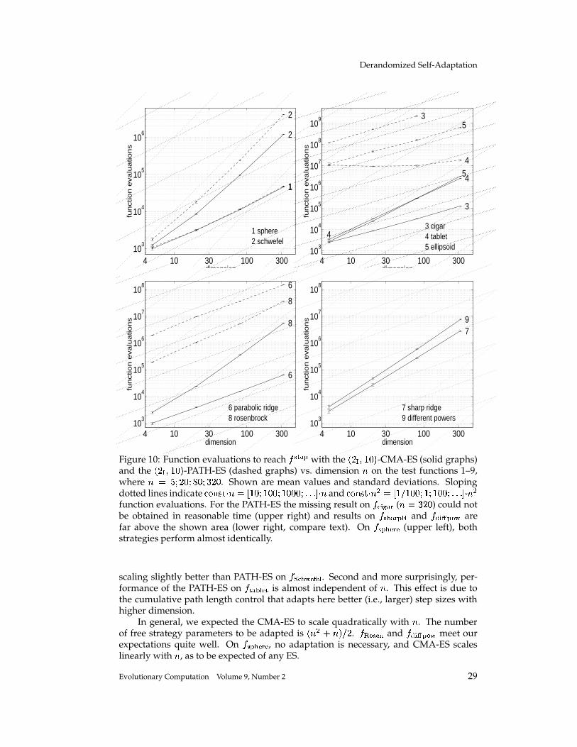
N. Hansen and A. Ostermeier

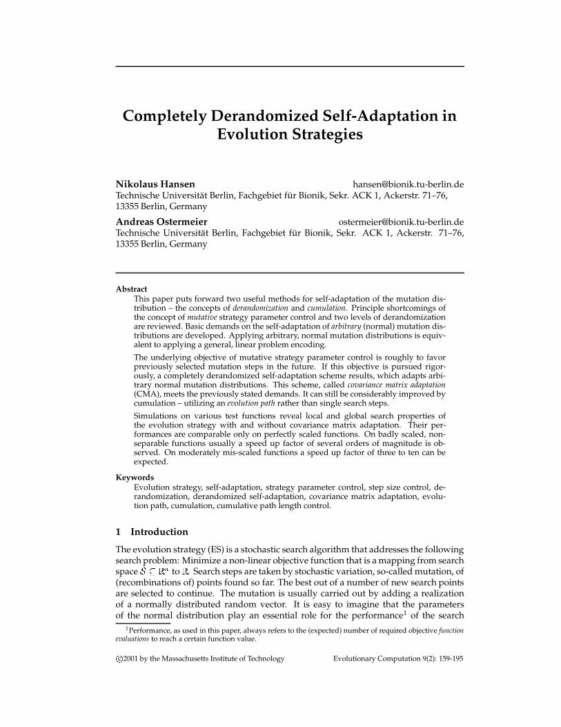
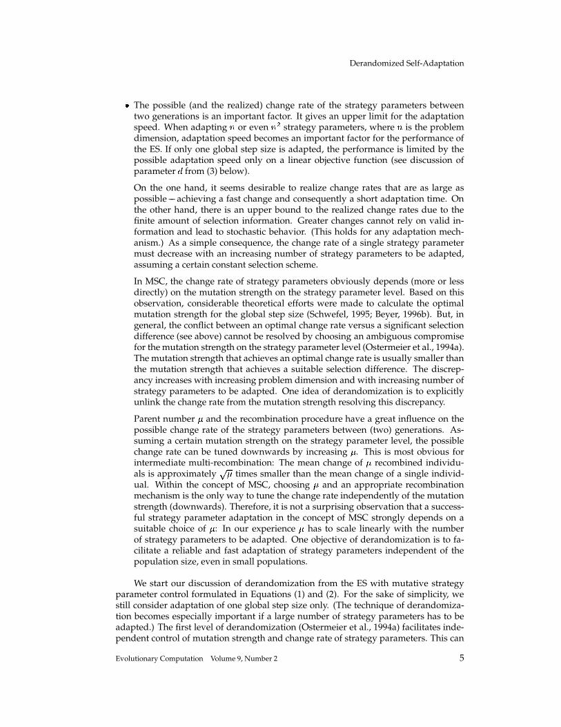
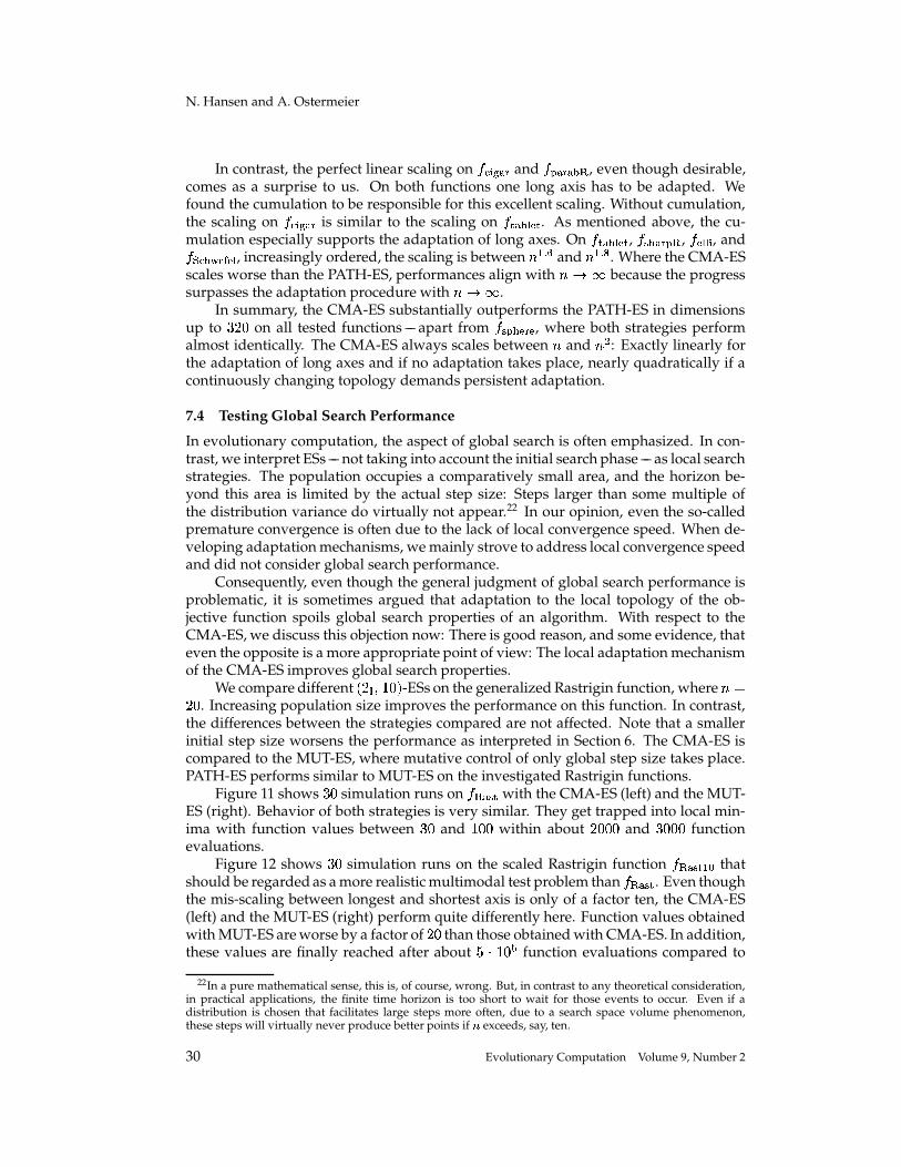
Figure 1: One- � lines of equal probability density of two normal distributions respec-tively. Left: one free parameter (circles). Middle: � free parameters (axis-parallel ellip-soids). Right:

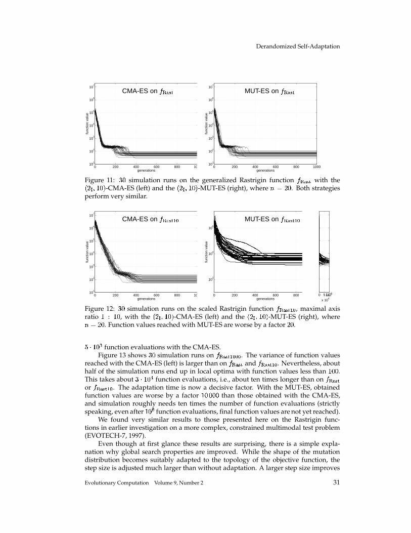
� �� free parameters (arbitrarily oriented ellipsoids).

algorithm. This paper is specifically concerned with the adjustment of the parametersof the normal mutation distribution.

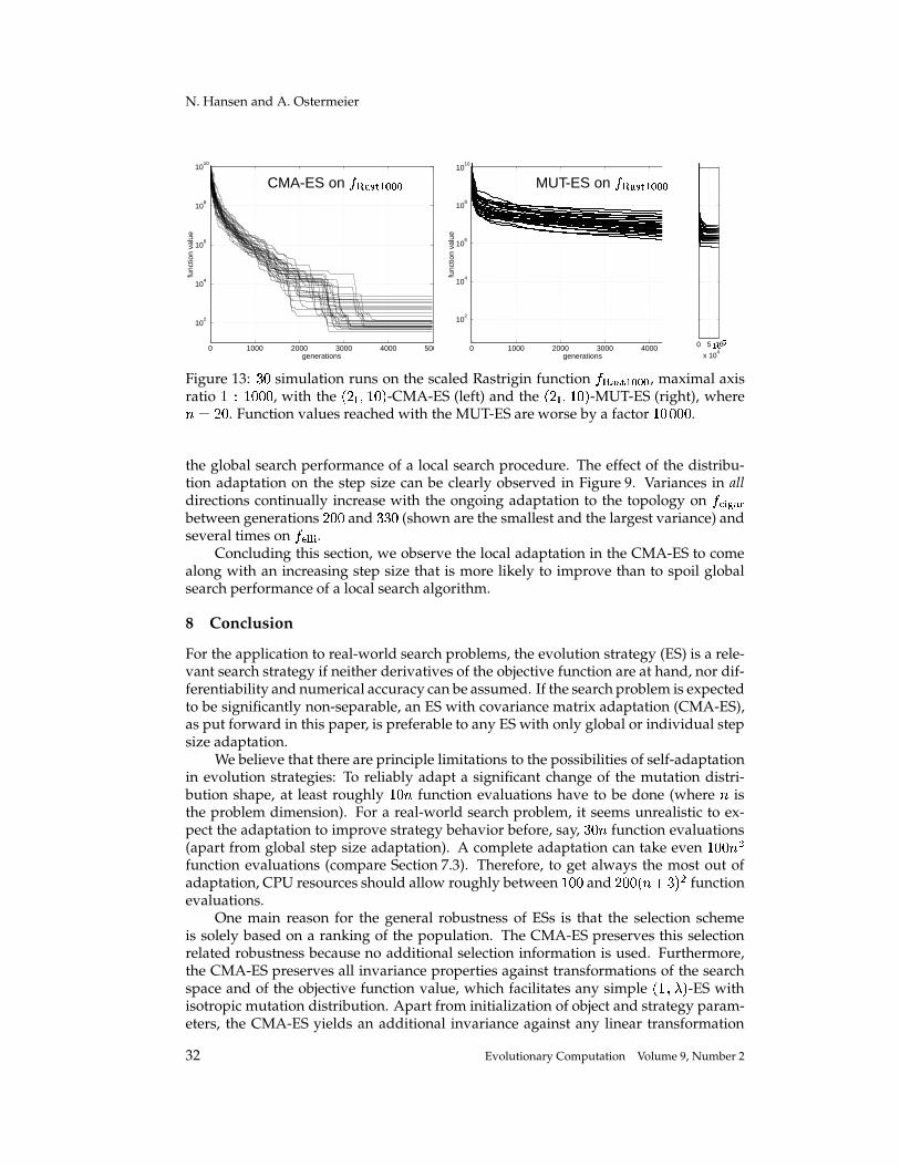
Among others, the parameters that parameterize the mutation distribution arecalled strategy parameters, in contrast to object parameters that define points in searchspace. Usually, no particularly detailed knowledge about the suitable choice of strat-egy parameters is available. With respect to the mutation distribution, there is typicallyonly a small width of strategy parameter settings where substantial search progresscan be observed (Rechenberg, 1973). Good parameter settings differ remarkably fromproblem to problem. Even worse, they usually change during the search process (pos-sibly by several orders of magnitude). For this reason, self-adaptation of the mutationdistribution that dynamically adapts strategy parameters during the search process isan essential feature in ESs.

We briefly review three consecutive steps of adapting normal mutation distribu-tions in ESs.

1. The normal distribution is chosen to be isotropic. Surfaces of equal probabilitydensity are circles (Figure 1, left), or (hyper-)spheres if �� . Overall variance ofthe distribution –– in other words the (global) step size or the expected step length ––is the only free strategy parameter.

2. The concept of global step size can be generalized.2 Each coordinate axis is as-signed a different variance (Figure 1, middle) –– often referred to as individual stepsizes. There are � free strategy parameters. The disadvantage of this concept is thedependency on the coordinate system. Invariance against rotation of the searchspace is lost. Why invariance is an important feature of an ES is discussed in Sec-tion 6.

3. A further generalization dynamically adapts the orthogonal coordinate system,where each coordinate axis is assigned a different variance (Figure 1, right). Anynormal distribution (with zero mean) can be produced. This concept results in

2There is more than one sensible generalization. For example, it is possible to provide one arbitrarilyoriented axis with a different variance. Then �� parameters have to be adapted. Such an adaptation canbe formulated independent of the coordinate system.

2 Evolutionary Computation Volume 9, Number 2

Derandomized Self-Adaptation

� � � � �� free strategy parameters. If an adaptation mechanism is suitably formu-lated, the invariance against rotations of search space is restored.

The adaptation of strategy parameters in ESs typically takes place in the concept ofmutative strategy parameter control (MSC). Strategy parameters are mutated, and a newsearch point is generated by means of this mutated strategy parameter setting.

We exemplify the concept formulating an� �� -ES with (purely) mutative control

of one global step size. �� and �� are the object parameter vector andstep size3 of the parent at generation � . The mutation step from generation � to � � �reads for each offspring ��

� � �� "! �$# � � (1)

� � �� % � �(2)

where:# � � , for �&� �'��(�

independent realizations of a random number withzero mean. Typically,

# � is normally distributed with standard deviation� ') � � (Back and Schwefel, 1993). We usually prefer to choose * �+# � �-, � � �.�* �$# � �0/1, � ��2� � �� (Rechenberg, 1994).

% �4365 �87 �:9 �; �� , for �<� �'��(�independent realizations of a

�87 �:9 � -normallydistributed random vector, where

9is the unity matrix. That is, components of% � are independent and identically� , �� -normally distributed.

After�

mutation steps are carried out, the best offspring (with respect to the ob-ject parameter vector � �� ) is selected to start the next generation step. Equation (1)facilitates the mutation on the strategy parameter level. The standard deviation of

#represents the mutation strength on the strategy parameter level.

This adaptation concept was introduced by Rechenberg (1973) for global and indi-vidual step sizes. Schwefel (1981) expanded the mutative approach to the adaptationof arbitrary normal mutation distributions, which is discussed in more detail in Section3.1. Ostermeier et al. (1994b) introduced a first level of derandomization into strategyparameter control that facilitates an individual step size adaptation in constantly smallpopulations. (If the standard mutative strategy parameter control is used to adapt in-dividual step sizes, based on our experience, the population size has to scale linearelywith the problem dimension � .)

In this paper, a second level of derandomization is put forward: The original objec-tive of mutative strategy parameter control –– that is to favor strategy parameter settingsthat produce selected steps with high probability (again) –– is explicitely realized. Com-plete derandomization, applied to the adaptation of arbitrary normal mutation distri-butions, leads almost inevitably to the covariance matrix adaptation (CMA) described inSection 3.2.

The paper is organized as follows. In Section 2, we discuss the basic shortcomingsof the concept of mutative strategy parameter control and review the derandomizedapproach to strategy parameter control in detail. In Section 3, the different concepts areinvestigated with respect to the adaptation of arbitrary normal mutation distributions.

3In this paper, step size always refers to = . Step size = is the component-wise standard deviationof the random vector =�>@?BA"C8D�EGFIHKJ . For this vector, ��=�L can be interpreted as overall variance andM�NPO =�>@?BA"C8D'E ORQ�S =�T � is the expected step length.

Evolutionary Computation Volume 9, Number 2 3


General demands on such an adaptation mechanism are developed, and the CMA-ESis introduced. In Section 4, the objective of strategy parameter control is expandedusing search paths (evolution paths) rather than single search steps as adaptation cri-terion. This concept is implemented by means of so-called cumulation. In Section 5,we formulate the CMA-ES algorithm, an evolution strategy that adapts arbitrary, nor-mal mutation distributions within a completely derandomized adaptation scheme withcumulation. Section 6 discusses the test functions used in Section 7, where various sim-ulation results are presented. In Section 8, a conclusion is given. Appendix A providesa MATLAB implementation of the CMA-ES.

2 Derandomization of Mutative Strategy Parameter Control

In the concept of mutative strategy parameter control (MSC), the selection probabil-ity of a strategy parameter setting is the probability to produce (with these strategyparameters) an object parameter setting that will be selected. Selection probability ofa strategy parameter setting can also be identified with its fitness. Consequently, weassume the following aim behind the concept of MSC:4 Find the strategy parameterswith the highest selection probability or, in other words, raise the probability of mu-tation steps that produced selected individuals.5 This implicitly assumes that strategyparameters that produced selected individuals before are suitable parameters in the(near) future. One idea of derandomization is to increase the probability of producingpreviously selected mutation steps again in a more direct way than MSC.

Before the concept of derandomization is discussed in detail, some importantpoints concerning the concept of MSC are reviewed.

� Selection of the strategy parameter setting is indirect. The selection process oper-ates on the object parameter adjustment. Comparing two different strategy para-meter settings, the better one has (only) a higher probability to be selected –– dueto object parameter realization. Differences between these selection probabilitiescan be quite small, that is, the selection process on the strategy parameter level ishighly disturbed. One idea of derandomization is to reduce or even eliminate thisdisturbance.

� The mutation on the strategy parameter level, as with any mutation, produces dif-ferent individuals that undergo selection. Mutation strength on the strategy para-meter level must ensure a significant selection difference between the individuals.In our view, this is the primary task of the mutation operator.

� Mutation strength on the strategy parameter level is usually kept constantthroughout the search process. Therefore, the mutation operator (on the strategyparameter level) must facilitate an effective mutation strength that is virtually in-dependent of the actual position in strategy parameter space. This can be compli-cated, because the best distance measure may not be obvious, and the position-independent formulation of a mutation operator can be difficult (see Section 3.1).

4We assume there is one best strategy parameter setting at each time step. Alternatively, to apply differentparameter settings at the same time means to challenge the idea of a normal search distribution. We foundthis alternative to be disadvantageous.

5Maximizing the selection probability is, in general, not identical with maximizing a progress rate. This isone reason for the often observed phenomenon that the global step size is adapted to be too small by MSC.This problem is addressed in the path length control (Equations (16) and (17)) by the so-called cumulation(Section 4).



� The possible (and the realized) change rate of the strategy parameters betweentwo generations is an important factor. It gives an upper limit for the adaptationspeed. When adapting � or even �� strategy parameters, where � is the problemdimension, adaptation speed becomes an important factor for the performance ofthe ES. If only one global step size is adapted, the performance is limited by thepossible adaptation speed only on a linear objective function (see discussion ofparameter

�from (3) below).

On the one hand, it seems desirable to realize change rates that are as large aspossible –– achieving a fast change and consequently a short adaptation time. Onthe other hand, there is an upper bound to the realized change rates due to thefinite amount of selection information. Greater changes cannot rely on valid in-formation and lead to stochastic behavior. (This holds for any adaptation mech-anism.) As a simple consequence, the change rate of a single strategy parametermust decrease with an increasing number of strategy parameters to be adapted,assuming a certain constant selection scheme.

In MSC, the change rate of strategy parameters obviously depends (more or lessdirectly) on the mutation strength on the strategy parameter level. Based on thisobservation, considerable theoretical efforts were made to calculate the optimalmutation strength for the global step size (Schwefel, 1995; Beyer, 1996b). But, ingeneral, the conflict between an optimal change rate versus a significant selectiondifference (see above) cannot be resolved by choosing an ambiguous compromisefor the mutation strength on the strategy parameter level (Ostermeier et al., 1994a).The mutation strength that achieves an optimal change rate is usually smaller thanthe mutation strength that achieves a suitable selection difference. The discrep-ancy increases with increasing problem dimension and with increasing number ofstrategy parameters to be adapted. One idea of derandomization is to explicitlyunlink the change rate from the mutation strength resolving this discrepancy.

Parent number � and the recombination procedure have a great influence on thepossible change rate of the strategy parameters between (two) generations. As-suming a certain mutation strength on the strategy parameter level, the possiblechange rate can be tuned downwards by increasing � . This is most obvious forintermediate multi-recombination: The mean change of � recombined individu-als is approximately ) � times smaller than the mean change of a single individ-ual. Within the concept of MSC, choosing � and an appropriate recombinationmechanism is the only way to tune the change rate independently of the mutationstrength (downwards). Therefore, it is not a surprising observation that a success-ful strategy parameter adaptation in the concept of MSC strongly depends on asuitable choice of � : In our experience � has to scale linearly with the numberof strategy parameters to be adapted. One objective of derandomization is to fa-cilitate a reliable and fast adaptation of strategy parameters independent of thepopulation size, even in small populations.

We start our discussion of derandomization from the ES with mutative strategyparameter control formulated in Equations (1) and (2). For the sake of simplicity, westill consider adaptation of one global step size only. (The technique of derandomiza-tion becomes especially important if a large number of strategy parameters has to beadapted.) The first level of derandomization (Ostermeier et al., 1994a) facilitates inde-pendent control of mutation strength and change rate of strategy parameters. This can



be achieved by slight changes in the formulation of the mutation step. For �� '��(�,

� � �� !� # �

�� (3)

� � �� "! �+# � � % � �(4)

where� �

is the damping parameter, and the symbols from Equations (1) and (2)in Section 1 are used. This can still be regarded as a mutative approach to strategyparameter control: If

� � �, Equations (3) and (4) are identical to (1) and (2), because

�� "! �8# � � in Equation (4) equals � � �� in Equation (2). Enlarging the damping para-meter

�reduces the change rate between � �� and � � �� leaving the selection relevant

mutation strength on the strategy parameter level (the standard deviation of# � in Equa-

tion (4)) unchanged. Instead of choosing the standard deviation to be� ) �� and

� � �,

as in the purely mutative approach, it is more sensible to choose the standard deviation� �� and� �� , assuming � � , facilitating the same rate of change with a larger

mutation strength. Large values for�

scale down fluctuations that occur due to stochas-tic effects, but decrease the possible change rate. For standard deviation

� �� within theinterval

�� , neither the fluctuations for small�

nor the limited change ratefor large

�decisively worsen the performance on the sphere objective function �� .

But if � or even �� strategy parameters have to be adapted, the trade-off between largefluctuations and a large change rate come the fore. Then the change rate must be tunedcarefully.

As Rechenberg (1994) and Beyer (1998) pointed out, this concept –– mutating bigand inheriting small –– can easily be applied to the object parameter mutation as well.It will be useful in the case of distorted selection on the object parameter level and isimplicitly implemented by intermediate multi-recombination.

In general, the first level of derandomization yields the following effects:� Mutation strength (in our example, standard deviation of

# � ) can be chosen com-paratively large in order to reduce the disturbance of strategy parameter selection.

� The ratio between change rate and mutation strength can be tuned downwards (inour example, by means of

�) according to the problem dimension and the number

of strategy parameters to be adapted. This scales down stochastic fluctuations ofthe strategy parameters.

� � and�

can be chosen independent of the adaptation mechanism. They, in partic-ular, become independent of the number of strategy parameters to be adapted.

The second level of derandomization completely removes the selection distur-bance on the strategy parameter level. To achieve this, mutation on the strategy para-meter level by means of sampling the random number

# � in Equation (3) is omitted.Instead, the realized step length � % � is used to change � . This leads to

� � �� "!� � % � � /�� 5 � 7 �(9 ��

� � (5)

� � �� % � (6)

� % � � /�� 5 �87 �(9 �� in Equation (5) replaces# � in Equation (3). Note that �� 5 �+7 �:9 ��

is the expectation of � % � � under random selection.6 Equation (5) is not intended to6Random selection occurs if the objective function returns random numbers independent of ! .



be used in practice, because the selection relevance of � % � � vanishes for increasing � .7

One can interpret Equation (5) as a special mutation on the strategy parameter levelor as an adaptation procedure for � (which must only be done for selected individu-als). Now, all stochastic variation of the object parameters –– namely originated by therandom vector realization % � in Equation (6) –– is used for strategy parameter adapta-tion in Equation (5). In other words, the actually realized mutation step on the objectparameter level is used for strategy parameter adjustment. If � % � � is smaller than ex-pected, �� is decreased. If � % � � is larger than expected � � �� is increased. Selecting asmall/large mutation step directly leads to reduction/enlargement of the step size.

The disadvantage of Equation (5) compared to Equation (1) is that it cannot beexpanded easily for the adaptation of other strategy parameters. The expansion to theadaptation of all distribution parameters is the subject of this paper.

In general, the completely derandomized adaptation follows the following princi-ples:

1. The mutation distribution is changed, so that the probability to produce the se-lected mutation step (again) is increased.

2. There is an explicit control of the change rate of strategy parameters (in our exam-ple, by means of

�).

3. Under random selection, strategy parameters are stationary. In our example, ex-pectation of �� equals �� .

In the next section, we discuss the adaptation of all variances and covariances of themutation distribution.

3 Adapting Arbitrary Normal Mutation Distributions

We give two motivations for the adaptation of arbitrary normal mutation distributionswith zero mean.

� The suitable encoding of a given problem is crucial for an efficient search withan evolutionary algorithm.8 Desirable is an adaptive encoding mechanism. Torestrict such an adaptive encoding/decoding to linear transformations seems rea-sonable: Even in the linear case, � � �� parameters have to be adapted. It is easyto show that in the case of additive mutation, linear transformation of the searchspace (and search points accordingly) is equivalent to linear transformation of themutation distribution. Linear transformation of the

� 7 �(9 � -normal mutation dis-tribution always yields a normal distribution with zero mean, while any normaldistribution with zero mean can be produced by a suitable linear transformation.This yields equivalence between an adaptive general linear encoding/decodingand the adaptation of all distribution parameters in the covariance matrix.

� We assume the objective function to be non-linear and significantly non-separable –– otherwise the search problem is comparatively easy, because it canbe solved by solving � one-dimensional problems. Adaptation to non-separableobjective functions is not possible if only individual step sizes are adapted. This

7For an efficient, completely derandomized global step size adaptation, the evolution path �� ? �� E�� ?�� E�� , where � ��? � �!��E#"$�%"&� � ��? �� :E , must be used instead of � � in Equation (5).This method is referred to as cumulative path length control and implemented with Equations (16) and (17).

8In biology, this is equivalent to a suitable genotype-phenotype transformation.



demands a more general mutation distribution and suggests the adaptation of ar-bitrary normal mutation distributions.

Choosing the mean value to be zero seems to be self-evident and is in accordancewith Beyer and Deb (2000). The current parents must be regarded as the best approxi-mation to the optimum known so far. Using nonzero mean is equivalent to moving thepopulation to another place in parameter space. This can be interpreted as extrapola-tion. We feel extrapolation is an anti-thesis to a basic paradigm of evolutionary com-putation. Of course, compared to simple ESs, extrapolation should gain a significantspeed up on many test functions. But, compared to an ES with derandomized strategyparameter control of the complete covariance matrix, the advantage from extrapolationseems small. Correspondingly, we find algorithms with nonzero mean (Ostermeier,1992; Ghozeil and Fogel, 1996; Hildebrand et al., 1999) unpromising.

In our opinion, any adaptation mechanism that adapts a general linear encod-ing/decoding has to meet the following fundamental demands:

Adaptation: The adaptation must be successful in the following sense: After an adap-tation phase, progress-rates comparable to those on the (hyper-)sphere objectivefunction � �� must be realized on any convex-quadratic objective function.9 Thismust hold especially for large problem conditions (greater than

� ,�� ) and non-systematically oriented principal axes of the objective function.

Performance: The performance (with respect to objective function evaluations) on the(hyper-)sphere function should be comparable to the performance of the

� �� -ESwith optimal step size, where �� , � � � .10 A loss by a factor up toten seems to be acceptable.

Invariance: The invariance properties of the� �� -ES with isotropic mutation distribu-

tion with respect to transformation of object parameter space and function valueshould be preserved. In particular, translation, rotation, and reflection of objectparameter space (and initial point accordingly) should have no influence on strat-egy behavior as well as any strictly monotonically increasing, i.e., order-preservingtransformation of the objective function value.

Stationarity: To get a reasonable strategy behavior in cases of low selection pressure,some kind of stationarity condition on the strategy parameters should be fulfilledunder purely random selection. This is analogous to choosing the mean valueto be zero for the object parameter mutation. At least non-stationarity must bequantified and judged.

From a conceptual point of view, one primary aim of strategy parameter adapta-tion is to become invariant (modulo initialization) against certain transformations ofthe object parameter space. For any fitness function

�� , the globalstep size adaptation can yield invariance against

�� , . An adaptive general linear9That is any function �� !! " !$#&% ! �!'(# ! �� , where the Hessian matrix % F H J�)�J is symmetric and

positive definite, ' F1HKJ and ��F1H . Due to numerical requirements, the condition of % may be restricted to,e.g., �+* �, . We use the expectation of J �.-0/ ?+?�� 1(2�354 �6�87�E ��?9� � � � �1(2:354 �6��7�E+E with ; F�< as the progress measure(where � 7 is the fitness value at the optimum), because it yields comparable values independent of % , ' ,� , � , and ; . For % � D and large � , this measure yields values close to the common normalized progressmeasure =?>@� � JACBED�F ?5G � � � M�N G �� Q E (Beyer, 1995), where G is the distance to the optimum.

10Not taking into account weighted recombination, the theoretically optimal ? � � �:E -ES yields approxi-mately *IH �J* .



encoding/decoding can additionally yield invariance against the full rank �� ma-trix

�. This invariance is a good starting point for achieving the adaptation demand.

Also, from a practical point of view, invariance is an important feature for assessing asearch algorithm (compare Section 6). It can be interpreted as a feature of robustness.Therefore, even to achieve an additional invariance seems to be very attractive.

Keeping in mind the stated demands, we discuss two approaches to the adaptationof arbitrary normal mutation distributions in the next two sections.

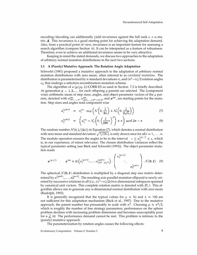
3.1 A (Purely) Mutative Approach: The Rotation Angle Adaptation

Schwefel (1981) proposed a mutative approach to the adaptation of arbitrary normalmutation distributions with zero mean, often referred to as correlated mutations. Thedistribution is parameterized by � standard deviations � � and

� � � / �� rotation angles�� that undergo a selection-recombination-mutation scheme.The algorithm of a

�� -CORR-ES as used in Section 7.2 is briefly described.

At generation � � �'� � �� for each offspring � parents are selected. The (componentwise) arithmetic mean of step sizes, angles, and object parameter vectors of the � par-ents, denoted with � �� , � �� , and �� , are starting points for the muta-tion. Step sizes and angles read component wise

� � �� !� 5 �

, �� 5 � � , � �

� ) � � � (7)� � �� 5 � � , � � �

� �',�� / � (8)

The random number 5 � , �� in Equation (7), which denotes a normal distributionwith zero mean and standard deviation � � � � �� , is only drawn once for all ! � �'�� .The modulo operation ensures the angles to be in the interval / � � � �� , whichis, in our experience, of minor relevance. The chosen distribution variances reflect thetypical parameter setting (see Back and Schwefel (1993)). The object parameter muta-tion reads

� � �� #"%$ � � �� '& �)(**+ � � �� . . .

� � ��

,'--. � 5 �87 �:9 � (9)

The spherical 5 �87 �:9 � distribution is multiplied by a diagonal step size matrix deter-mined by � � �� . The resulting axis-parallel mutation ellipsoid is newly ori-ented by successive rotations in all (i.e.,

� � �'/�� ) two-dimensional subspaces spannedby canonical unit vectors. This complete rotation matrix is denoted with " � � � . This al-gorithm allows one to generate any � -dimensional normal distribution with zero mean(Rudolph, 1992).

It is generally recognized that the typical values for � � ��and

� � � ,�, arenot sufficient for this adaptation mechanism (Back et al., 1997). Due to the mutativeapproach, the parent number has presumably to scale with � � . Choosing � � � � � ,which is roughly the number of free strategy parameters, performance on the sphereproblem declines with increasing problem dimension and becomes unacceptably poorfor �0/� � , . The performance demand cannot be met. This problem is intrinsic to the(purely) mutative approach.

The parameterization by rotation angles causes the following effects:



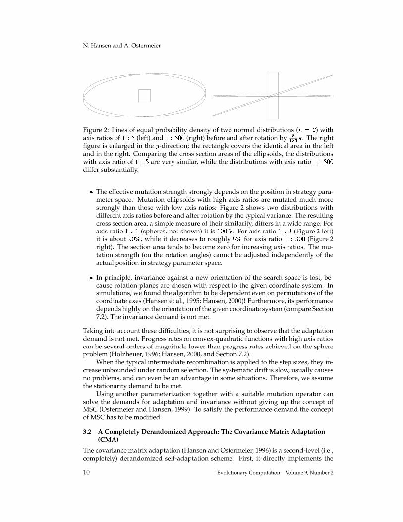
Figure 2: Lines of equal probability density of two normal distributions ( �<� � ) withaxis ratios of

� � � (left) and� � �',�, (right) before and after rotation by �� . The right

figure is enlarged in the � -direction; the rectangle covers the identical area in the leftand in the right. Comparing the cross section areas of the ellipsoids, the distributionswith axis ratio of

� � � are very similar, while the distributions with axis ratio� � �',�,

differ substantially.

� The effective mutation strength strongly depends on the position in strategy para-meter space. Mutation ellipsoids with high axis ratios are mutated much morestrongly than those with low axis ratios: Figure 2 shows two distributions withdifferent axis ratios before and after rotation by the typical variance. The resultingcross section area, a simple measure of their similarity, differs in a wide range. Foraxis ratio

� � �(spheres, not shown) it is

� ,�,�� . For axis ratio� � � (Figure 2 left)

it is about �',�� , while it decreases to roughly� � for axis ratio

� � ��,', (Figure 2right). The section area tends to become zero for increasing axis ratios. The mu-tation strength (on the rotation angles) cannot be adjusted independently of theactual position in strategy parameter space.

� In principle, invariance against a new orientation of the search space is lost, be-cause rotation planes are chosen with respect to the given coordinate system. Insimulations, we found the algorithm to be dependent even on permutations of thecoordinate axes (Hansen et al., 1995; Hansen, 2000)! Furthermore, its performancedepends highly on the orientation of the given coordinate system (compare Section7.2). The invariance demand is not met.

Taking into account these difficulties, it is not surprising to observe that the adaptationdemand is not met. Progress rates on convex-quadratic functions with high axis ratioscan be several orders of magnitude lower than progress rates achieved on the sphereproblem (Holzheuer, 1996; Hansen, 2000, and Section 7.2).

When the typical intermediate recombination is applied to the step sizes, they in-crease unbounded under random selection. The systematic drift is slow, usually causesno problems, and can even be an advantage in some situations. Therefore, we assumethe stationarity demand to be met.

Using another parameterization together with a suitable mutation operator cansolve the demands for adaptation and invariance without giving up the concept ofMSC (Ostermeier and Hansen, 1999). To satisfy the performance demand the conceptof MSC has to be modified.

3.2 A Completely Derandomized Approach: The Covariance Matrix Adaptation(CMA)

The covariance matrix adaptation (Hansen and Ostermeier, 1996) is a second-level (i.e.,completely) derandomized self-adaptation scheme. First, it directly implements the



aim of MSC to raise the probability of producing successful mutation steps: The covari-ance matrix of the mutation distribution is changed in order to increase the probabilityof producing the selected mutation step again. Second, the rate of change is adjustedaccording to the number of strategy parameters to be adapted (by means of

� �� inEquation (15)). Third, under random selection, the expectation of the covariance ma-trix

�is stationary. Furthermore, the adaptation mechanism is inherently independent

of the given coordinate system. In short, the CMA implements a principle componentanalysis of the previously selected mutation steps to determine the new mutation dis-tribution. We give an illustrative description of the algorithm.

Consider a special method to produce realizations of a � -dimensional normal dis-tribution with zero mean. If the vectors % � �� %�� , � � , span

��, and 5 � , ��

denotes independent� , �� -normally distributed random numbers, then

5 � , �� % � � �� 5 � , �� % � (10)

is a normally distributed random vector with zero mean.11 Choosing % � , ! � �� ,appropriate any normal distribution with zero mean can be realized.

The distribution in Equation (10) is generated by adding the “line distributions”5 � , �� % � 3 5 �87 � % � %�� . If the vector % � is given, the normal (line) distribution withzero mean, which produces the vector % � with the highest probability (density) of allnormal distributions with zero mean, is 5 �87 � % � %� � � . (The proof is simple and omitted.)

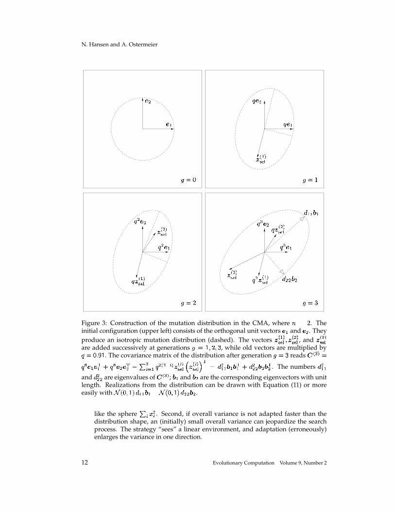
The covariance matrix adaptation (CMA) constructs the mutation distribution outof selected mutation steps. In place of the vectors % � in Equation (10), the selectedmutation steps are used with exponentially decreasing weights. An example is shownin Figure 3, where � � � . The isotropic initial distribution is constructed by means ofthe unit vectors � and � . At every generation � � �� , the selected mutation step% �� is added to the vector tuple. All other vectors are multiplied by a factor � � �

.12

According to Equation (10), after generation �@� � , the distribution reads

5 � , �� 5 � , �� 5� , �� % � � �� 5 � , �� % � �(�� 5 � , �� % � � �� (11)

This mutation distribution tends to reproduce the mutation steps selected in thepast generations. In the end, it leads to an alignment of the distributions before and af-ter selection, i.e., an alignment of the recent mutation distribution with the distributionof the selected mutation steps. If both distributions become alike, as under randomselection, in expectation, no further change of the distributions takes place (Hansen,1998).

This illustrative but also formally precise description of the CMA differs in threepoints from the CMA-ES formalized in Section 5. These extensions are as follows:

� Apart from the adaptation of the distribution shape, the overall variance of themutation distribution is adapted separately. We found the additional adaptationof the overall variance useful for at least two reasons. First, changes of the overallvariance and of the distribution shape should operate on different time scales. Dueto the number of parameters to be adapted, the adaptation of the covariance ma-trix, i.e., the adaptation of the distribution shape, must operate on a time scale of� � . Adaptation of the overall variance should operate on a time scale � , because thevariance should be able to change as fast as required on simple objective functions

11The covariance matrix of this normally distributed random vector reads � � # � H H+H�� #� .12 � adjusts the change rate, and � L corresponds to �#� �� in Equation (15).



�

�

� �-,

��

��

% � � ��

� � �

� � �

� � �

� % � � ��

% � �:��

� � �

� � �

� � �

� � % � � ��

� % � �(��

% � � ��

� ��

��

� � �

Figure 3: Construction of the mutation distribution in the CMA, where �0� � . Theinitial configuration (upper left) consists of the orthogonal unit vectors � and � . Theyproduce an isotropic mutation distribution (dashed). The vectors % � � �� % � �(�� , and % � � �� are added successively at generations � � �'� � � � , while old vectors are multiplied by��-, � � � . The covariance matrix of the distribution after generation �� reads

� � � � �� % � � �� $ % � � �� & � � � � ��

�� . The numbers

� � ��and

� �� are eigenvalues of� � � � ; � � and

�� are the corresponding eigenvectors with unit

length. Realizations from the distribution can be drawn with Equation (11) or moreeasily with 5 � , �� 5 � , ��

� �� .

like the sphere � � � �� . Second, if overall variance is not adapted faster than thedistribution shape, an (initially) small overall variance can jeopardize the searchprocess. The strategy “sees” a linear environment, and adaptation (erroneously)enlarges the variance in one direction.



� The CMA is formulated for parent number �� and weighted multi-recombina-

tion, resulting in a more sophisticated computation of % �� .� The technique of cumulation is applied to the vectors, that construct the distribu-

tion. Instead of the single mutation steps % � �� , evolution paths � �� are used. Anevolution path � �� represents a sequence of selected mutation steps. The tech-nique of cumulation is motivated in the next section.

The adaptation scheme is formalized by means of the covariance matrix of thedistribution, because storing as many as � vectors is not practicable. That is, in everygeneration � , after selection of the best search points has taken place,

1. The covariance matrix of the new distribution� � �� is calculated due to

� � � � � andthe vector % � �� (with cumulation � �� ). In other words, the covariance matrix of thedistribution is adapted.

2. Overall variance is adapted by means of the cumulative path length control. Re-ferring to Equation (5), % � is replaced by a “conjugate” evolution path (�� in Equa-tions (16) and (17)).

3. From the covariance matrix, the principal axes of the new distribution and theirvariances are calculated. To produce realizations from the new distribution the �line distributions are added, which correspond to the principal axes of the muta-tion distribution ellipsoid (compare Figure 3).

Storage requirements are � � �� . We note, that “generally, for any moderate � , this isan entirely trivial disadvantage” (Press et al., 1992). For computational and numericalrequirements, refer to Sections 5.2 and 7.1.

4 Utilizing the Evolution Path: Cumulation

The concept of MSC utilizes selection information of a single generation step. In con-trast, it can be useful to utilize a whole path taken by the population over a number ofgenerations. We call such a path an evolution path of the ES. The idea of the evolutionpath is similar to the idea of isolation. The performance of a strategy can be evaluatedsignificantly better after a couple of steps are taken than after a single step. It is worthnoting that both quantity and quality of the evaluation basis can improve.

Accordingly, to reproduce successful evolution paths seems more promising thanto reproduce successful single mutation steps. The former is more likely to maximizea progress rate while the latter emphasizes the selection probability. Consequently,we expand the idea of strategy parameter control: The adaptation should maximizethe probability to reproduce successful, i.e., actually taken, evolution paths rather thansingle mutation steps (Hansen and Ostermeier, 1996).

An evolution path contains additional selection information compared to singlesteps – correlations between single steps successively taken in the generation sequenceare utilized. If successively selected mutation steps are parallel correlated (scalar prod-uct greater than zero), the evolution path will be comparatively long. If the steps areanti-parallel correlated (scalar product less than zero), the evolution path will be com-paratively short. Parallel correlation means that successive steps are going in the samedirection. Anti-parallel correlation means that the steps cancel each other out. Weassume both correlations to be inefficient. This is most obvious if the correlation/anti-correlation between successive steps is perfect. These steps can exactly be replacedwith the enlarged/reduced first step.



�

��

�

� �/ � / �

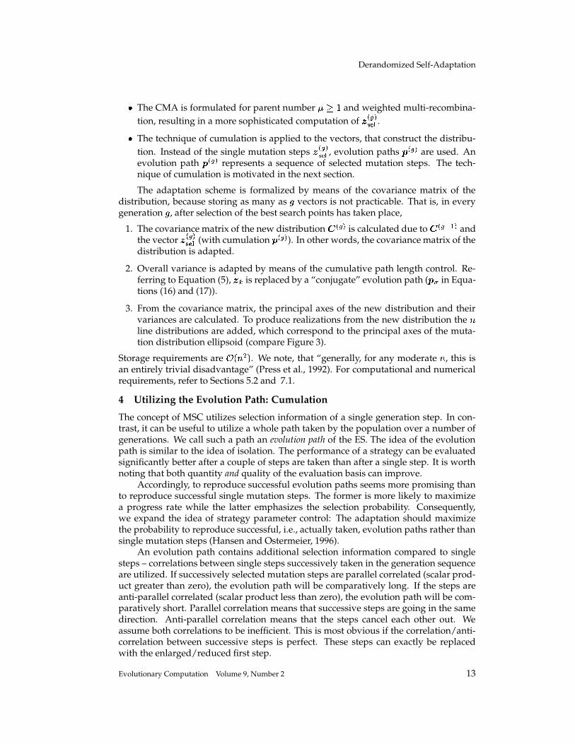
Figure 4: Two idealized evolution paths (solid) in a ridge topography (dotted). Thedistributions constructed by the single steps (dashed, reduced in size) are identical.

Consequently, to maximize mutation step efficiency, it is necessary to realize longersteps in directions where the evolution path is long –– here the same distance can be cov-ered by fewer but longer steps. On the other side, it is appropriate to realize shortersteps in directions where the evolution path is short. Both can be achieved using evo-lution paths rather than single mutation steps for the construction of the mutation dis-tribution as described in Section 3.2.

We calculate an evolution path within an iterative process by (weighted) summa-tion of successively selected mutation steps. The evolution path � � � obeys

� � �� / � � � �� ./ � � % � �� (12)

where , � � �and � � � �2� 7

. This procedure, introduced in Ostermeier et al. (1994b),is called cumulation. � �� / � � is a normalization factor: Assuming % � �� and � ��in Equation (12) to be independent and identically distributed yields �� 3 � ��independently of

� � ,�� . Variances of � � �� and � �� are identical because� �<�� / � � � � � �� / � � � . If

� � �, no cumulation takes place, and � � �� % � �� . The life

span of information accumulated in � �� is roughly� � (Hansen, 1998): After about

� �generations the original information in � �� is reduced by the factor

� � � , � �� . Thatmeans

� � �can roughly be interpreted as the number of summed steps.

The benefit from cumulation is shown with an idealized example. Consider thetwo different sequences of four consecutive generation steps in Figure 4. Compare anyevolution path, that is, any sum of consecutive steps in the left and in the right of thefigure. They differ significantly with respect to direction and length. Notice that thedifference is only due to the sign of vectors two and four.

Construction of a distribution from the single mutation steps (single vectors inthe figure) according to Equation (10) leads to exactly the same result in both cases(dashed). Signs of constructing vectors do not matter, because the vectors are multi-plied by a

� , �� -normally distributed random number that is symmetrical about zero.The situation changes when cumulation is applied. We focus on the left of Figure 4.

Consider a continuous sequence of the shown vectors –– i.e., an alternating sequence ofthe two vectors � and � . Then % � � � � � �� and % � � � �� for ! � �'� � �� , and accordingto Equation (12), the evolution path � �� alternately reads

� �� / � � $ � � � � / � � � � � � / � � � � � � � / � � � � � �� / � � � � % � � �� &14 Evolutionary Computation Volume 9, Number 2


�� S �JH �

� � S�� H � � � S�� H � � � � �+*

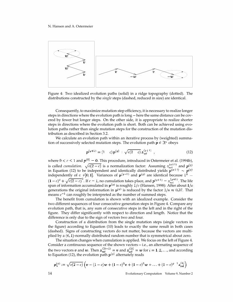
Figure 5: Resulting cumulation vectors � � and �� and distribution ellipsoids for analternating selection of the two vectors � and � from Figure 4, left. For

� � �, no

cumulation takes place, and � � � � and �� (upper left). Shown is the result forvalues of

� � � � � � ) �� ) � , � ) ��, � ) � ,', , respectively.

at odd generation number � and

� �� / � � $ � � � � / � � � � � � / � � � � � � � / � �� / � � � � % � � �� &at even generation number. For � �� we get

� ��

� � � � / � �� / � � � � and

� ��

� � � � / � �� / � � � �

After � � generations, the deviation from these limits is under� � .

To visualize the effect of cumulation, these vectors and the related distributions areshown in Figure 5 for different values of

�. With increasing life span

� � �, the vectors � �

and � � become more and more similar. The distribution scales down in the horizontaldirection, increasing in the vertical direction. Already for a life span of approximatelythree generations, the effect appears to be very substantial. Notice again that this effect



is due to correlations between consecutive steps. This information cannot be detectedutilizing single mutation steps separately. Because additional information is evaluated,cumulation can make adaptation of the distribution parameters faster and more reliable.

In our research, we repeatedly found cumulation to be a very useful concept. Inthe following CMA-ES algorithm, we use cumulation in two places: primarily for thecumulative path length control, where cumulation takes place in Equation (16), and thestep size � is adapted from the generated evolution path � � in Equation (17); second,for the adaptation of the mutation distribution as exemplified in this section and takingplace in Equation (14).

5 The��

-CMA-ES Algorithm

We formally describe an evolution strategy utilizing the methods illustrated in Sections3.2 and 4, denoted by CMA-ES.13 Based on a suggestion by Ingo Rechenberg (1998),weighted recombination from the � best out of

�individuals is applied, denoted with�

�� .14 Weighted recombination is a generalization of intermediate multi-recombi-nation, denoted

�� , where all recombination weights are identical. A MATLAB

implementation of the�

� � � � � -CMA-ES algorithm is given in Appendix A.The transition from generation � to � � �

of the parameters � �� ,� �� ,

� �� , � �� , and � ��1 � � , as written in Equations (13) to (17),completely defines the algorithm. Initialization is � � � �� 7

and� � � � � 9

(unitymatrix), while the initial object parameter vector �+�� and the initial step size � � � � haveto be chosen problem dependent. All vectors are assumed to be column vectors.

The object parameter vector � � �� of individual �@� �'��(�reads

� � �� +�� <�� % � �� "! � # BED�F � �(13)

where the following apply:

� � �� , object parameter vector of the � %$ individual in generation � � �.

�+�� &(')+*-,/. ) �10� ��2 � � ��43 , 2 � � � , weighted mean of the � best individuals of

generation � . The index ! � � denotes the ! %$ best individual.�� , step size in generation � . � � � � is the initial component wise standard

deviation of the mutation step.% � �� , for � � �'��(�and � � , �� independent realizations of a

�87 �:9 � -normally distributed random vector. Components of % � �� are independent� , �� -normally distributed.� �� Symmetrical positive definite � � � -matrix.

� �� is the covariance matrix ofthe normally distributed random vector � �� 5 � 7 �(9 � . � �� determines� �� and � �� . � �� 65 � �� 87 � � � ��95 � � ��:7 � 5 � � ��:7 � , whichis a singular value decomposition of

� � �� . Initialization� � � � � 9

.

13The algorithm described here is identical to the algorithms in Hansen and Ostermeier (1996) setting; � � , � � � �=< , and >�< � ?�@ACB ; in Hansen and Ostermeier (1997) setting D � H+H H � DFE , � � � �=< and> < � G ; and in Hansen (1998) setting D � H+H+H � D E .14This notation follows Beyer (1995), simplifying the ? ; � ;�H CJI'E -notation for intermediate multi-recombi-

nation to ? ;�H C:I'E , avoiding the misinterpretation of ; and ;KH being different numbers.



� �� -diagonal matrix (step size matrix).� � � � , for ! �� and diagonal

elements� � �� of � �� are square roots of eigenvalues of the covariance matrix� �� .� �� orthogonal � � � -matrix (rotation matrix) that determines the coordinate sys-

tem, where the scaling with � �� takes place. Columns of � �� are (definedas) the normalized eigenvectors of the covariance matrix

� �� . The ! %$ di-

agonal element of � �� squared� �� is the corresponding eigenvalue to the! %$ column of � �� , � �� . That is,� �� for ! � �'�� . � is

orthogonal, i.e., � � � � � � .

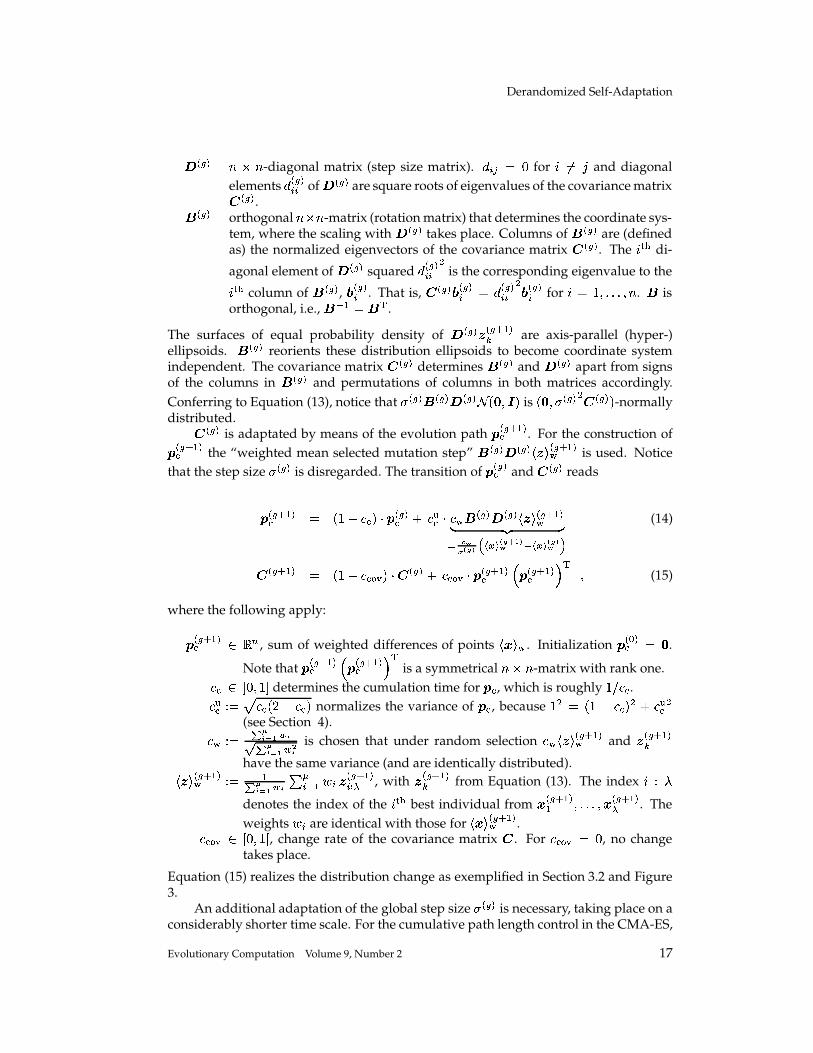
The surfaces of equal probability density of � �� % � �� are axis-parallel (hyper-)ellipsoids. � �� reorients these distribution ellipsoids to become coordinate systemindependent. The covariance matrix

� �� determines � �� and � �� apart from signsof the columns in � � �� and permutations of columns in both matrices accordingly.Conferring to Equation (13), notice that � �� 5 � 7 �(9 � is

�87 � �� -normallydistributed.� �� is adaptated by means of the evolution path � � �� . For the construction of� � �� the “weighted mean selected mutation step” � �� % � � �� is used. Noticethat the step size � �� is disregarded. The transition of � � �� and

� �� reads

� � �� / � � � � � �� % � � �� B D�F�� B D��, F� � � �� B D�F��

(14)

� � �� / � �� $ � � �� & � �(15)


� � �� , sum of weighted differences of points �8�� . Initialization � � � �� 7.

Note that � � �� $ � � �� & � is a symmetrical � � � -matrix with rank one.� � � , �� determines the cumulation time for � � , which is roughly� � � .� �� / � � � normalizes the variance of � � , because

� � � � � / � � � � � � �� (see Section 4).� � � � & ') *�,/. )) & ')+*-,/. �) is chosen that under random selection

� � � % � � �� and % � �� have the same variance (and are identically distributed).

� % � � �� & ')+*-, . ) � 0� ��2 � % � �� 3 , with % � �� from Equation (13). The index ! � �denotes the index of the ! %$ best individual from � � �� . Theweights 2 � are identical with those for �+�� .� �� , �� , change rate of the covariance matrix

�. For

� �� , , no changetakes place.

Equation (15) realizes the distribution change as exemplified in Section 3.2 and Figure3.

An additional adaptation of the global step size � �� is necessary, taking place on aconsiderably shorter time scale. For the cumulative path length control in the CMA-ES,



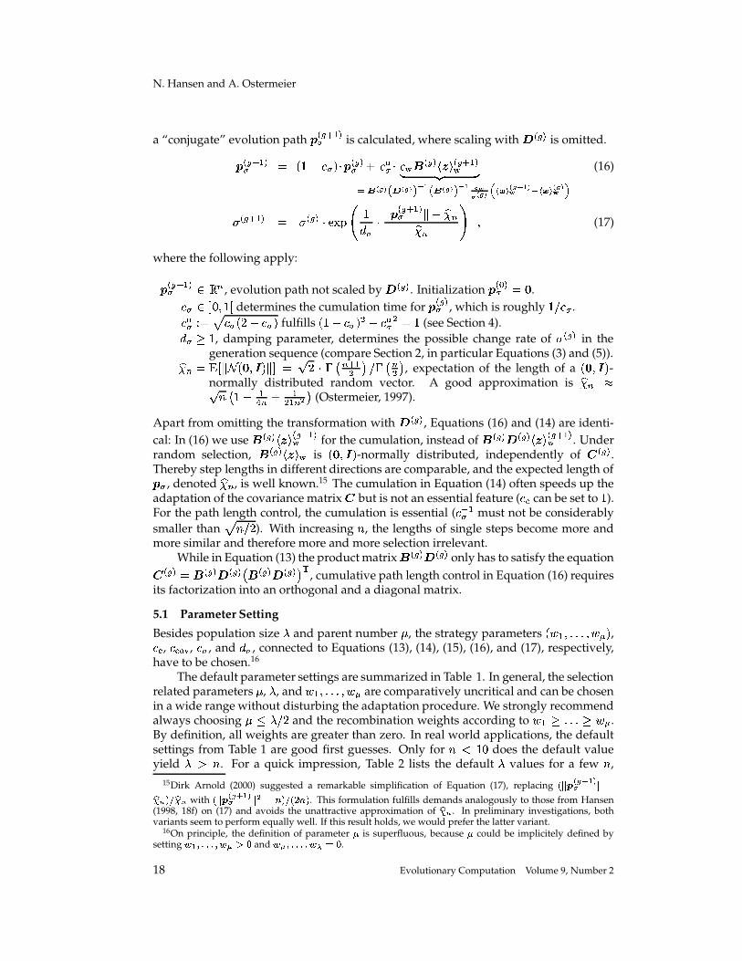
a “conjugate” evolution path � � �� is calculated, where scaling with � �� is omitted.

� � �� / ��

�� % � � �� BED�F �� B D�F � � , � � BED�F � � , � �� B D�F � �� BED�� , F� � � � � BED�F��

(16)

� � �� "!� �

��

� � � � �� / ��

� �(17)


� � �� , evolution path not scaled by � �� . Initialization � � � �� 7.�

� � , �� determines the cumulation time for � � �� , which is roughly� � � .� �

��

�� / �

� � fulfills� � / �

� � ��

(see Section 4).��

, damping parameter, determines the possible change rate of � �� in thegeneration sequence (compare Section 2, in particular Equations (3) and (5)).�� 5 � 7 �(9 � �� ) � �� 5 � �� 7 � 5 � � 7 , expectation of the length of a

� 7 �(9 � -normally distributed random vector. A good approximation is

�� ) � 5 � / �

� � �� 7 (Ostermeier, 1997).

Apart from omitting the transformation with � �� , Equations (16) and (14) are identi-cal: In (16) we use � �� % � � �� for the cumulation, instead of � �� % � � �� . Underrandom selection, � �� % � � is

�87 �:9 � -normally distributed, independently of� �� .

Thereby step lengths in different directions are comparable, and the expected length of� � , denoted

�� , is well known.15 The cumulation in Equation (14) often speeds up theadaptation of the covariance matrix

�but is not an essential feature (

� � can be set to�).

For the path length control, the cumulation is essential (� �K�� must not be considerably

smaller than � � �� ). With increasing � , the lengths of single steps become more andmore similar and therefore more and more selection irrelevant.

While in Equation (13) the product matrix � �� only has to satisfy the equation� �� 65 � �� :7 � , cumulative path length control in Equation (16) requiresits factorization into an orthogonal and a diagonal matrix.

5.1 Parameter Setting

Besides population size�

and parent number � , the strategy parameters� 2 � �� 2 0 � ,� � , � �� ,

�� , and

�� , connected to Equations (13), (14), (15), (16), and (17), respectively,

have to be chosen.16

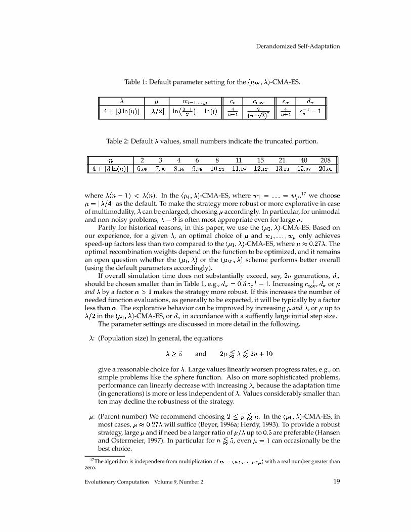
The default parameter settings are summarized in Table 1. In general, the selectionrelated parameters � ,

�, and 2 � �� 2 0 are comparatively uncritical and can be chosen

in a wide range without disturbing the adaptation procedure. We strongly recommendalways choosing �

� �� and the recombination weights according to 2 � �� 2 0 .By definition, all weights are greater than zero. In real world applications, the defaultsettings from Table 1 are good first guesses. Only for � � � , does the default valueyield

� / � . For a quick impression, Table 2 lists the default�

values for a few � ,15Dirk Arnold (2000) suggested a remarkable simplification of Equation (17), replacing ? O � � � ��< O �

J E�� J with ? O � �� < O L � ��E��?�� "E . This formulation fulfills demands analogously to those from Hansen(1998, 18f) on (17) and avoids the unattractive approximation of

J . In preliminary investigations, bothvariants seem to perform equally well. If this result holds, we would prefer the latter variant.

16On principle, the definition of parameter ; is superfluous, because ; could be implicitely defined bysetting D C HCH H C"D E�� * and D E CCH H H C"D� � * .



Table 1: Default parameter setting for the�

� � � � � -CMA-ES.

�� 2 �� 0 � � � ��

�� 5 �� 7 / �� ! � ��'� � ��

� � ��

Table 2: Default�

values, small numbers indicate the truncated portion.

� 2 3 4 6 8 11 15 21 40 208� �� 5� � �� , � �+� �� I� � � � �', � ��where

� � � / � � � � � �� . In the�

�� -CMA-ES, where 2 � � �� 2 0 ,17 we choose� �� as the default. To make the strategy more robust or more explorative in caseof multimodality,

�can be enlarged, choosing � accordingly. In particular, for unimodal

and non-noisy problems,� � � is often most appropriate even for large � .

Partly for historical reasons, in this paper, we use the�

� � � � � -CMA-ES. Based onour experience, for a given

�, an optimal choice of � and 2 � �� 2 0 only achieves

speed-up factors less than two compared to the�

� � � � � -CMA-ES, where � � , � � � � . Theoptimal recombination weights depend on the function to be optimized, and it remainsan open question whether the

�� or the

�� scheme performs better overall

(using the default parameters accordingly).If overall simulation time does not substantially exceed, say, � � generations,

��

should be chosen smaller than in Table 1, e.g.,��@� , �0� � �K��

. Increasing� � �� ,

�� or �

and�

by a factor � / �makes the strategy more robust. If this increases the number of

needed function evaluations, as generally to be expected, it will be typically by a factorless than � . The explorative behavior can be improved by increasing � and

�, or � up to� �� in the

�� -CMA-ES, or

�� in accordance with a suffiently large initial step size.

The parameter settings are discussed in more detail in the following.�

: (Population size) In general, the equations

� �and � �

�� ,give a reasonable choice for

�. Large values linearly worsen progress rates, e.g., on

simple problems like the sphere function. Also on more sophisticated problems,performance can linearly decrease with increasing

�, because the adaptation time

(in generations) is more or less independent of�

. Values considerably smaller thanten may decline the robustness of the strategy.

� : (Parent number) We recommend choosing � �

�� . In the�

�� -CMA-ES, inmost cases, � � , � � � � will suffice (Beyer, 1996a; Herdy, 1993). To provide a robuststrategy, large � and if need be a larger ratio of � � up to , �0� are preferable (Hansenand Ostermeier, 1997). In particular for � ��

, even � � �can occasionally be the

best choice.

17The algorithm is independent from multiplication of � � ? D CCH H+H C"D E E with a real number greater thanzero.



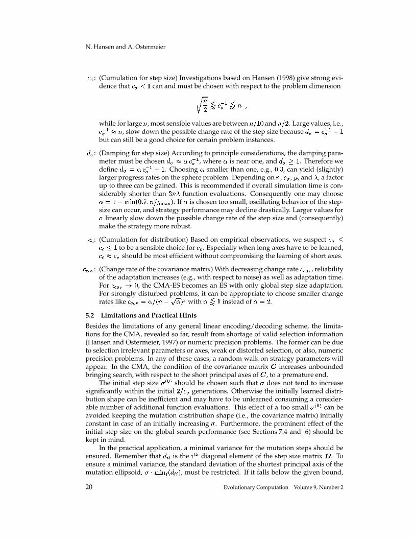
�� : (Cumulation for step size) Investigations based on Hansen (1998) give strong evi-

dence that��

can and must be chosen with respect to the problem dimension� ��

��

��

while for large � , most sensible values are between � � , and � � . Large values, i.e.,� �K��

� � , slow down the possible change rate of the step size because��

� � �but can still be a good choice for certain problem instances.

�� : (Damping for step size) According to principle considerations, the damping para-

meter must be chosen�� K�� , where � is near one, and

��

. Therefore wedefine

��

. Choosing � smaller than one, e.g., , � � , can yield (slightly)larger progress rates on the sphere problem. Depending on � ,

�� , � , and

�, a factor

up to three can be gained. This is recommended if overall simulation time is con-siderably shorter than � � � function evaluations. Consequently one may choose� � � / �� , � � � � �� . If � is chosen too small, oscillating behavior of the step-size can occur, and strategy performance may decline drastically. Larger values for� linearly slow down the possible change rate of the step size and (consequently)make the strategy more robust.

� � : (Cumulation for distribution) Based on empirical observations, we suspect��

� � �

to be a sensible choice for� � . Especially when long axes have to be learned,� � � �

� should be most efficient without compromising the learning of short axes.� �� : (Change rate of the covariance matrix) With decreasing change rate

� �� , reliabilityof the adaptation increases (e.g., with respect to noise) as well as adaptation time.For

� �� , , the CMA-ES becomes an ES with only global step size adaptation.For strongly disturbed problems, it can be appropriate to choose smaller changerates like

� �� ) � � � with � �� instead of � �� .

5.2 Limitations and Practical Hints

Besides the limitations of any general linear encoding/decoding scheme, the limita-tions for the CMA, revealed so far, result from shortage of valid selection information(Hansen and Ostermeier, 1997) or numeric precision problems. The former can be dueto selection irrelevant parameters or axes, weak or distorted selection, or also, numericprecision problems. In any of these cases, a random walk on strategy parameters willappear. In the CMA, the condition of the covariance matrix

�increases unbounded

bringing search, with respect to the short principal axes of�

, to a premature end.The initial step size � � � � should be chosen such that � does not tend to increase

significantly within the initial � � � generations. Otherwise the initially learned distri-bution shape can be inefficient and may have to be unlearned consuming a consider-able number of additional function evaluations. This effect of a too small � � � � can beavoided keeping the mutation distribution shape (i.e., the covariance matrix) initiallyconstant in case of an initially increasing � . Furthermore, the prominent effect of theinitial step size on the global search performance (see Sections 7.4 and 6) should bekept in mind.

In the practical application, a minimal variance for the mutation steps should beensured. Remember that

� �� is the ! "$ diagonal element of the step size matrix � . Toensure a minimal variance, the standard deviation of the shortest principal axis of themutation ellipsoid, � � �� , must be restricted. If it falls below the given bound,



step size � should be enlarged (compare Appendix A). Problem specific knowledgemust be used for setting the bound. Numerically, a lower limit is given by the demand�+�� +�� , � � � � � �� for each unit vector � . With respect to the selectionprocedure, even

� � �8�� +�� , � � � � � �� seems desirable.To avoid numerical errors, a maximal condition number for

� �� , e.g.,� , � � , should

be ensured. If the ratio between the largest and smallest eigenvalue of� � �� exceeds� , � � , the operation

� �� , � �"/ �� 9 limits the conditionnumber in a reasonable way to

� , � �� .

The numerical stability of computing eigenvectors and eigenvalues of the symmet-rical matrix

�usually poses no problems. In MATLAB, the built-in function eig can be

used. To avoid complex solutions, the symmetry of�

must be explicitly enforced (com-pare Appendix A). In C/C++, we used the functions tred2 and tqli from Press etal. (1992), substituting float with double and setting the maximal iteration numberin tqli to ��,�� . Another implementation was done in Turbo-PASCAL. For conditionnumbers up to

� , � � , we never observed numerical problems in any of these program-ming languages.

If the user decides to manually change object parameters during the search pro-cess – which is not recommended – the adaptation procedure (Equations (14) to (17))must be omitted for these steps. Otherwise, the strategy parameter adaptation can beseverely disturbed.

Because change of� �� is comparatively slow (time scale �� ), it is possible to up-

date � �� and � �� not after every generation but after ) � or even after, e.g., � � , gen-erations. This reduces the computational effort of the strategy from � � � � � to � � � � � � � or� � � � � , respectively. The latter corresponds to the computational effort for a fixed linearencoding/decoding of the problem as well as for producing a realization of an (arbi-trarily) normally distributed, random vector on the computer. In practical applications,it is often most appropriate to update � �� and � �� every generation.

A simple method to handle constraints repeats the generation step, defined inEquation (13), until

�or at least � feasible points are generated before Equations (14)

to (17) are applied. If the initial mutation distribution generates sufficiently numer-ous feasible solutions, this method can remain sufficient during the search process dueto the symmetry of the mutation distribution. If the minimum searched for is locatedat the edge of the feasible region, the performance will usually be poor and a moresophisticated method should be used.

6 Test Functions

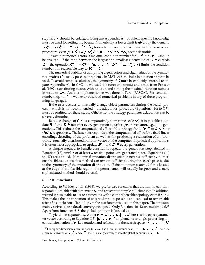
According to Whitley et al. (1996), we prefer test functions that are non-linear, non-separable, scalable with dimension � , and resistant to simple hill-climbing. In addition,we find it reasonable to use test functions with a comprehensible topology even if � �� .This makes the interpretation of observed results possible and can lead to remarkablescientific conclusions. Table 3 gives the test functions used in this paper. The test suitemainly strives to test (local) convergence speed. Only functions10–12 are multimodal.18

Apart from functions 6–8, the global optimum is located at7

.To yield non-separability, we set � � � � � � �� , where � is the object parame-

ter vector according to Equation (13). � � � �� implements an angle-preserving lin-ear transformation of � , i.e., rotation and reflection of the search space. � � ��

18For higher dimension, even function 8 �� 392�� has a local minimum near � � ? � ��C��C+H H+H C �:E # . With thegiven initialization of �!� � � �� and = � � � , the ES usually converges into the global minimum at � �� .



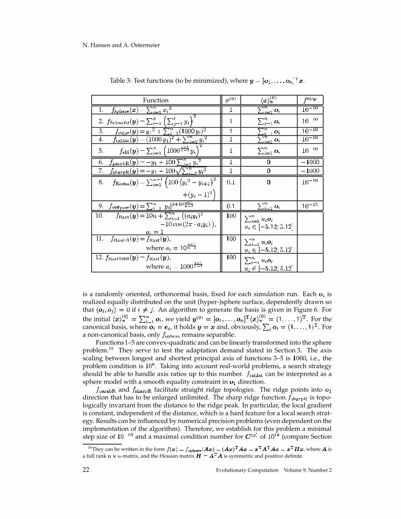
Table 3: Test functions (to be minimized), where � � � � � �� .

Function �� +��

1.� �� $ � � � � � �� , � � �

2.�� $ � ��E�� $ � �� & � � � �� , � � �

3.� �� ,',�, � � � � � � �� , � � �

4.� � �� ,',�, � � � � � � �� , � � �

5.� �� $ � ,',�, ) � ,B � , � � & � � � �� , � � �

6.� � � � �� 6/ � � � � ,�, � �� 7 / � ,',�,

7.� � $ � �� 6/ � � � � ,�, � � �� 7 / � ,',�,

8.� � � �� $ � ,', 5 � � � / � � �� 7 �

� � � � / � � � & , � � 7 � , � � �9.

�� ) � ,B � , , � � � �� , � � �10.

� � �� , � � � �� 5 �� / � ,�� 7 ,� � � �

� ,', � �� / �"� � �� "� � ��

11.� � �� ,

where� � � � ,

)�,B � ,

� ,', � �� / �"� � �� "� � ��

12.� � �� ,

where� � � � ,',�,

)�,B � ,

� ,', � �� / �"� � �� "� � ��

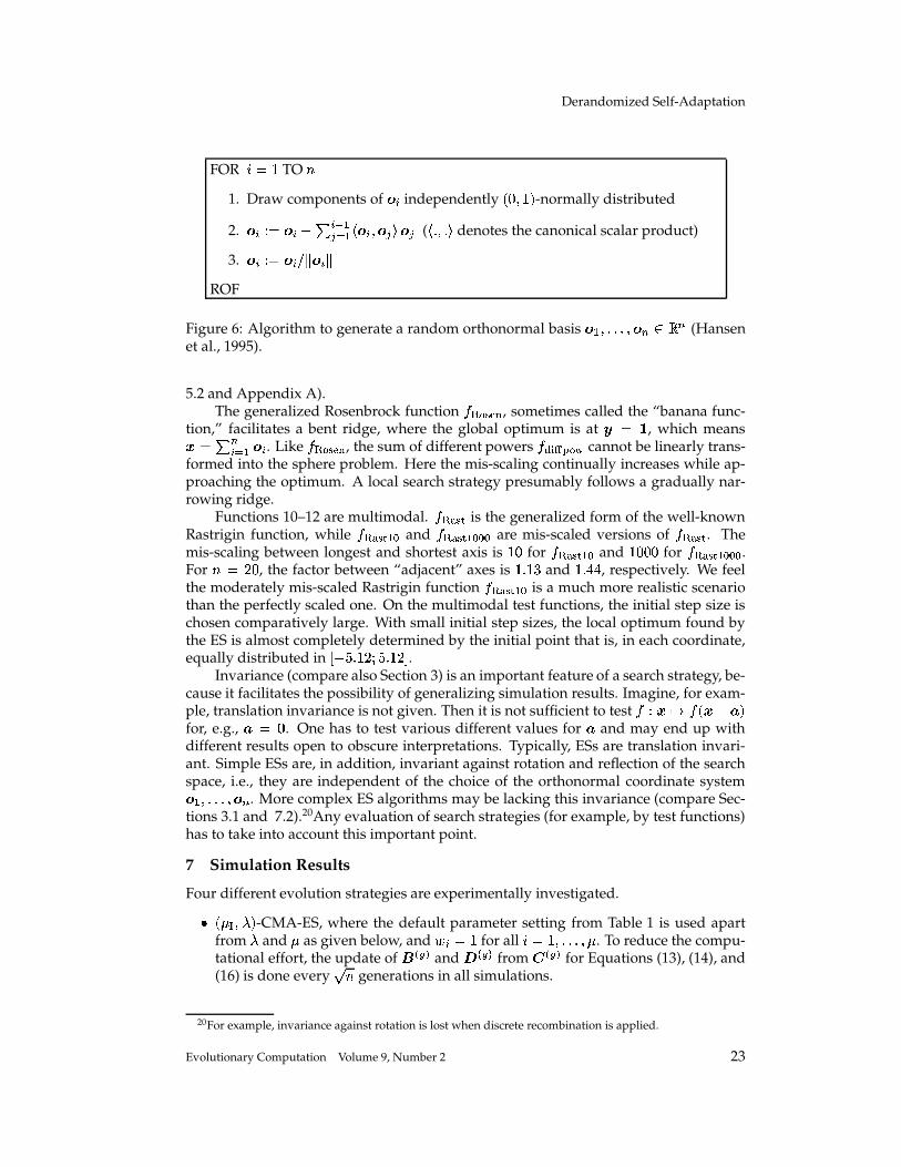
is a randomly oriented, orthonormal basis, fixed for each simulation run. Each � � isrealized equally distributed on the unit (hyper-)sphere surface, dependently drawn sothat � � � � � � �.� , if ! �� . An algorithm to generate the basis is given in Figure 6. Forthe initial �+�� , we yield �2� � � � � � � �� +�� '�� . For thecanonical basis, where � � � � , it holds �6� � and, obviously, � � � � � � �'�� . Fora non-canonical basis, only

� �� $ remains separable.Functions1–5 are convex-quadratic and can be linearly transformed into the sphere

problem.19 They serve to test the adaptation demand stated in Section 3. The axisscaling between longest and shortest principal axis of functions 3–5 is

� ,�,', , i.e., theproblem condition is

� , � . Taking into account real-world problems, a search strategyshould be able to handle axis ratios up to this number.

� � � � can be interpreted as asphere model with a smooth equality constraint in � � direction.� � � � �� and

� �%$ � �� facilitate straight ridge topologies. The ridge points into � �direction that has to be enlarged unlimited. The sharp ridge function

� � $ � �� is topo-logically invariant from the distance to the ridge peak. In particular, the local gradientis constant, independent of the distance, which is a hard feature for a local search strat-egy. Results can be influenced by numerical precision problems (even dependent on theimplementation of the algorithm). Therefore, we establish for this problem a minimalstep size of

� , � � � and a maximal condition number for� �� of

� , � � (compare Section

19They can be written in the form � ?�! E � � 3�� 2 �92 ?"! ! E � ?"! ! E�#�! ! � ! #�! ##! ! � ! # % ! , where ! isa full rank �%$ � -matrix, and the Hessian matrix % � ! # ! is symmetric and positive definite.



FOR ! � �TO �

1. Draw components of � � independently� , �� -normally distributed

2. � � � � � � / � � � �� ( � � �� denotes the canonical scalar product)

3. � � � � � � � � � �ROF

Figure 6: Algorithm to generate a random orthonormal basis � � �� (Hansenet al., 1995).

5.2 and Appendix A).The generalized Rosenbrock function

� � � �� , sometimes called the “banana func-tion,” facilitates a bent ridge, where the global optimum is at � �� , which means�6� � �� . Like

� � � �� , the sum of different powers� � �� cannot be linearly trans-

formed into the sphere problem. Here the mis-scaling continually increases while ap-proaching the optimum. A local search strategy presumably follows a gradually nar-rowing ridge.

Functions 10–12 are multimodal.� � �� is the generalized form of the well-known

Rastrigin function, while� � �� and

� � �� are mis-scaled versions of� � �� . The

mis-scaling between longest and shortest axis is� , for

� � �� and� ,�,', for

� � �� .For �-� �', , the factor between “adjacent” axes is

�'� � � and�� , respectively. We feel

the moderately mis-scaled Rastrigin function� � �� is a much more realistic scenario

than the perfectly scaled one. On the multimodal test functions, the initial step size ischosen comparatively large. With small initial step sizes, the local optimum found bythe ES is almost completely determined by the initial point that is, in each coordinate,equally distributed in � / �"� � �� .

Invariance (compare also Section 3) is an important feature of a search strategy, be-cause it facilitates the possibility of generalizing simulation results. Imagine, for exam-ple, translation invariance is not given. Then it is not sufficient to test

� � � �� /�� for, e.g., �0� 7

. One has to test various different values for � and may end up withdifferent results open to obscure interpretations. Typically, ESs are translation invari-ant. Simple ESs are, in addition, invariant against rotation and reflection of the searchspace, i.e., they are independent of the choice of the orthonormal coordinate system� � �� . More complex ES algorithms may be lacking this invariance (compare Sec-tions 3.1 and 7.2).20Any evaluation of search strategies (for example, by test functions)has to take into account this important point.

7 Simulation Results

Four different evolution strategies are experimentally investigated.

��

�� -CMA-ES, where the default parameter setting from Table 1 is used apartfrom

�and � as given below, and 2 � � �

for all ! � �'�� . To reduce the compu-

tational effort, the update of � �� and � �� from� �� for Equations (13), (14), and

(16) is done every ) � generations in all simulations.

20For example, invariance against rotation is lost when discrete recombination is applied.



�� I� � � �� ,', � -CORR-ES (correlated mutations), an ES with rotation angle adapta-tion according to Section 3.1. The initialization of the rotation angles is randomlyuniform between / � and � , identical for all initial individuals.

�� , � -PATH-ES, the same strategy as the

� � � �� , � -CMA-ES, while� �� is set to

zero.� �� 9

for all �@� , ��'� � �� , and therefore, � � �� and � �� can be set to9. Equations (14) and (15) become superfluous, and only cumulative path length

control takes place.�� , � -MUT-ES, an ES with mutative adaptation of one (global) step size and in-termediate recombination on object and strategy parameters as in CORR-ES. Mu-tation on the strategy parameter level is carried out as in Equation (1), where

# � is� , �� ') � � � � -normally distributed.

In the beginning of Section 3, we formulated four fundamental demands on analgorithm that adapt a general linear encoding in ESs. Now we pursue the questionwhether the CMA-ES can satisfy these demands.

The invariance demand is met because the algorithm is formulated inherently in-dependent of the coordinate system: All results of CMA-ES, PATH-ES, and MUT-ESare independent of the basis � � �� actually chosen (see Section 6), i.e., valid forany orthonormal coordinate system. That means, these strategies are, in particular,independent of rotation and reflection of the search space.

The performance demand is also satisfied. The� � � � � � -CMA-ES performs on

� � � $ between

�� ( � large) and � ( �6� �

) times slower than the� �� -ES with isotropic mu-

tation distribution and optimal step size. The applicability of the CMA algorithm isindependent of any reasonable choice of � and

�.

The stationarity demand is respected because, under random selection, expecta-tion of

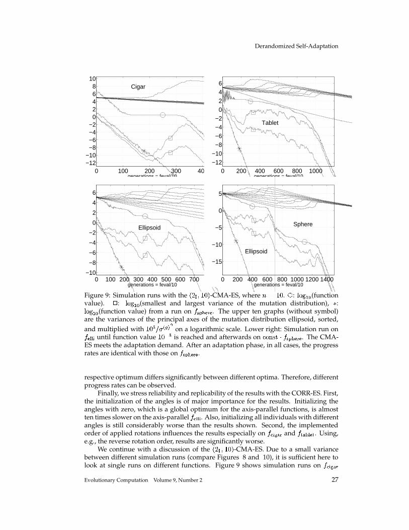
� � �� equals� �� , and expectation of �� equals �� (Hansen, 1998).

Simulation runs on functions 3–5 in Section 7.2 will show that the adaptation de-mand is met as well.

In Section 7.3, performance results on the unimodal test functions 1–9 are pre-sented, and scaling properties are discussed. In Section 7.4, global search propertiesare evaluated.

7.1 CPU-Times

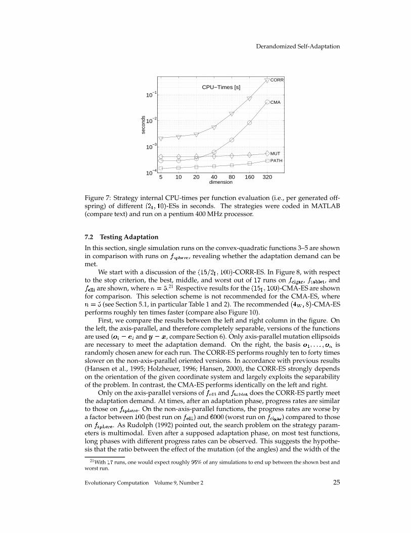
We think strategy internal time consumption is of minor relevance. It seems needless tosay that results strongly depend on implementational skills and the programming lan-guage chosen. Nevertheless, to complete the picture, we summarize CPU-times takenby strategy internal operations of different

� � � �� , � -ESs in Figure 7. The strategies werecoded in MATLAB and run uncompiled on a pentium 400 MHz processor. Differencesbetween MUT-ES and PATH-ES are presumably due to the more sophisticated recom-bination operator in MUT-ES, which allows two parent recombination independent ofthe parent number � . MATLAB offers relatively efficient routines for the most time con-suming computations in the CMA-ES. Therefore, even for � �� ', , the CMA-ES needsonly

� , ms CPU-time per generated offspring. This time can still be reduced doing theupdate of � �� and � �� every � � , generations instead of every ) � generations. Noefficient MATLAB routines are available for the rotation procedure in the CORR-ES. Tomake CPU-times comparable, this procedure was reimplemented in C and called fromMATLAB gaining a remarkable speed up. CORR-ES is still seven to ten times slowerthan CMA-ES. This may be due to a trivial implementational matter and does not makeany difference for many non-linear, non-separable search problems.



5 10 20 40 80 160 32010

−4

10−3

10−2

10−1

CPU−Times [s]

PATH

MUT

CMA

CORR

dimension

seco

nds

Figure 7: Strategy internal CPU-times per function evaluation (i.e., per generated off-spring) of different

� �� , � -ESs in seconds. The strategies were coded in MATLAB(compare text) and run on a pentium 400 MHz processor.

7.2 Testing Adaptation

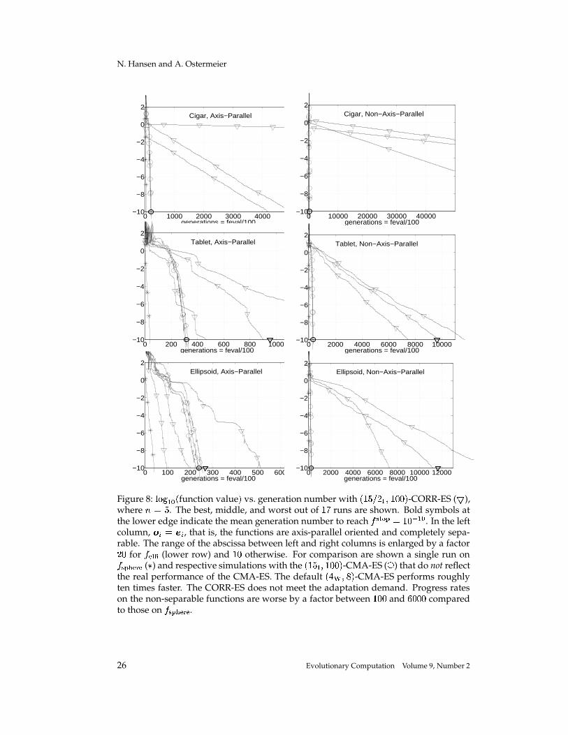
In this section, single simulation runs on the convex-quadratic functions 3–5 are shownin comparison with runs on

� �� $ , revealing whether the adaptation demand can bemet.

We start with a discussion of the� �I� �� ,', � -CORR-ES. In Figure 8, with respect

to the stop criterion, the best, middle, and worst out of� � runs on

� �� , � � � � , and� �� are shown, where � � �.21 Respective results for the

� �� ,�, � -CMA-ES are shownfor comparison. This selection scheme is not recommended for the CMA-ES, where� � �

(see Section 5.1, in particular Table 1 and 2). The recommended� � � � � � -CMA-ES

performs roughly ten times faster (compare also Figure 10).First, we compare the results between the left and right column in the figure. On

the left, the axis-parallel, and therefore completely separable, versions of the functionsare used ( � � � � and � � � , compare Section 6). Only axis-parallel mutation ellipsoidsare necessary to meet the adaptation demand. On the right, the basis � � �� israndomly chosen anew for each run. The CORR-ES performs roughly ten to forty timesslower on the non-axis-parallel oriented versions. In accordance with previous results(Hansen et al., 1995; Holzheuer, 1996; Hansen, 2000), the CORR-ES strongly dependson the orientation of the given coordinate system and largely exploits the separabilityof the problem. In contrast, the CMA-ES performs identically on the left and right.

Only on the axis-parallel versions of� �� and

� � �� does the CORR-ES partly meetthe adaptation demand. At times, after an adaptation phase, progress rates are similarto those on

� � � $ . On the non-axis-parallel functions, the progress rates are worse bya factor between

� ,', (best run on� �� ) and ',�,', (worst run on

� �� ) compared to thoseon

� �� $ . As Rudolph (1992) pointed out, the search problem on the strategy param-eters is multimodal. Even after a supposed adaptation phase, on most test functions,long phases with different progress rates can be observed. This suggests the hypothe-sis that the ratio between the effect of the mutation (of the angles) and the width of the

21With � � runs, one would expect roughly � �� of any simulations to end up between the shown best andworst run.



0 1000 2000 3000 4000−10

−8

−6

−4

−2

0

2Cigar, Axis−Parallel

generations = feval/1000 10000 20000 30000 40000

−10

−8

−6

−4

−2

0

2Cigar, Non−Axis−Parallel

generations = feval/100

0 200 400 600 800 1000−10

−8

−6

−4

−2

0

2Tablet, Axis−Parallel

generations = feval/1000 2000 4000 6000 8000 10000

−10

−8

−6

−4

−2

0

2Tablet, Non−Axis−Parallel


0 100 200 300 400 500 600−10

−8

−6

−4

−2

0

2Ellipsoid, Axis−Parallel

generations = feval/1000 2000 4000 6000 8000 10000 12000

−10

−8

−6

−4

−2

0

2Ellipsoid, Non−Axis−Parallel


Figure 8: �� function value � vs. generation number with� �I� � � �� ,', � -CORR-ES ( � ),

where � � �. The best, middle, and worst out of

� � runs are shown. Bold symbols atthe lower edge indicate the mean generation number to reach

� �� , �K� � . In the leftcolumn, � � � � , that is, the functions are axis-parallel oriented and completely sepa-rable. The range of the abscissa between left and right columns is enlarged by a factor� , for

� �� (lower row) and� , otherwise. For comparison are shown a single run on� �� $ ( � ) and respective simulations with the

� �� '� ,', � -CMA-ES ( � ) that do not reflectthe real performance of the CMA-ES. The default

� � � � � � -CMA-ES performs roughlyten times faster. The CORR-ES does not meet the adaptation demand. Progress rateson the non-separable functions are worse by a factor between

� ,�, and �,',', comparedto those on

� �� $ .26 Evolutionary Computation Volume 9, Number 2


0 100 200 300 400−12−10−8−6−4−2

02468

10Cigar

generations = feval/100 200 400 600 800 1000

−12−10−8−6−4−2

0246

Tablet


0 100 200 300 400 500 600 700−10

−8

−6

−4

−2

0

2

4

6

Ellipsoid

generations = feval/100 200 400 600 800 1000 1200 1400

−15

−10

−5

0

5

Sphere

Ellipsoid


Figure 9: Simulation runs with the� �� '� , � -CMA-ES, where � � � , . � : �� (function

value). � : �� (smallest and largest variance of the mutation distribution), � :�� (function value) from a run on

� � � $ . The upper ten graphs (without symbol)are the variances of the principal axes of the mutation distribution ellipsoid, sorted,and multiplied with

� , � �� on a logarithmic scale. Lower right: Simulation run on� �� until function value� , � � is reached and afterwards on � �8� �� 8� �� $ . The CMA-

ES meets the adaptation demand. After an adaptation phase, in all cases, the progressrates are identical with those on

� �� $ .respective optimum differs significantly between different optima. Therefore, differentprogress rates can be observed.

Finally, we stress reliability and replicability of the results with the CORR-ES. First,the initialization of the angles is of major importance for the results. Initializing theangles with zero, which is a global optimum for the axis-parallel functions, is almostten times slower on the axis-parallel

� �� . Also, initializing all individuals with differentangles is still considerably worse than the results shown. Second, the implementedorder of applied rotations influences the results especially on

� �� and� � � � . Using,

e.g., the reverse rotation order, results are significantly worse.We continue with a discussion of the

� � � � � , � -CMA-ES. Due to a small variancebetween different simulation runs (compare Figures 8 and 10), it is sufficient here tolook at single runs on different functions. Figure 9 shows simulation runs on

� �� Evolutionary Computation Volume 9, Number 2 27


(upper left) and� � �� (upper right), where � � � , , compared to a run on

� �� $ . Theadaptation process can be clearly observed through the variances of the principle axesof the mutation distribution, where global step size is disregarded (upper ten graphs).When the variances correspond to the scaling in the objective function, progress ratesidentical to those on

� �� $ are realized (notice again that the basis � � �� is chosenrandomly here). The shorter adaptation time on

� �� is due to the cumulation, whichdetects the parallel correlations of single steps very efficiently.

In the lower left of Figure 9, a simulation run on� �� is shown. Similar to

� � � � ,but more pronounced, local adaptation occurs repeatedly on this function. Progressincreases and decreases a few times together with the step size. When the adaptationis completed, the variances are evenly spread in a range of

� , � . In the lower right ofFigure 9, the objective function is switched from

� �� to (some multiple of)� �� $ , after

reaching function value� , � � . The mutation distribution adapts from an ellipsoid-like

shape back to the isotropic distribution. Adaptation time and graphs of function valueand step size are very similar to those on

� �� . In fact, from a theoretical point of view,the algorithm must show exactly the same behavior in both adaptation cases (apartfrom stochastic influences). Again, after the adaptation phase, progress rates identicalto those on

� �� $ are achieved in both cases.Concluding these results, the adaptation demand is satisfied by the CMA-ES: Any

convex-quadratic function is rescaled into the sphere function.

7.3 Testing Convergence Speed and Scaling

In this section, we investigate the number of function evaluations to reach� ��

ontest functions 1–9, where � � � � �',�� ,�� , . The

� � � �'� , � -CMA-ES is compared to the� �� , � -PATH-ES, where only global step size adaptation takes place and which usually(slightly) outperforms the

� �� '� , � -MUT-ES. Depending on CPU-time resources, up to� , simulation runs are evaluated. Figure 10 shows the results on the convex-quadratictest functions 1–5 (first row). On

� �� $ , both strategies perform almost identically,while on

� � �"$ � �� , the results are still comparable (upper left). The difference on� � � $

is due to the decreasing variance of the covariance matrix supporting the adaptation ofthe step size � that is somewhat too slow (see above discussion of damping parameter�� in Section 5.1). If the axis ratio between the longest and shortest axis is

� � � ,',', ,as on

� �� , � � � � , and� �� (upper right), CMA-ES outperforms PATH-ES by a factor

between � (� � � � , � � � � , ) and almost ',�,',', (

� �� ). Only on� � � � for � / ��, does

the factor fall below� ,', .

The lower row of Figure 10 shows the results on functions 6–9. The CMA-ES worksquite well even on different kinds of ridge-like topologies. On

� � � �� , the CMA-ESis � – �', times faster than PATH-ES; on

� � � � �� , the factor becomes � ,�,', (lower left).Results for the PATH-ES on

� � $ � �� and�� #�� are omitted (lower right). On the latter,� ��

is reached after more than� , � � function evaluations ( � � �

). On the former, thePATH-ES does not reach

� � ��because step size converges to zero (as with mutative

step size control). Setting the minimum step size to� , � � � , far more than

� , � � functionevaluations are needed to reach

� �� .

We take an interesting look at the scaling properties with � (compare the slopinggrids in the figure). As with simple ESs in general, PATH-ES scales linearly on mostfunctions. There are two exceptions. First, on

� � �"$ � �� the PATH-ES scales quadrat-ically. The axis ratio between longest and shortest principal axis of this function in-creases with increasing � . That is, not only problem dimension but also “problem diffi-culty” increases. Therefore, a simple ES scales worse than linear. This favors CMA-ES



4 10 30 100 30010

3

104

105

106

11

2

2

fun

ctio

n e

va

lua

tio

ns

dimension

2 schwefel1 sphere

4 10 30 100 30010

3

104

105

106

107

108

109

3

3

4

4

45

5

fun

ctio

n e

va

lua

tio

ns

dimension

5 ellipsoid4 tablet3 cigar

4 10 30 100 30010

3

104

105

106

107

108

8

8

6

6

fun

ctio

n e

va

lua

tio

ns

dimension

8 rosenbrock6 parabolic ridge

4 10 30 100 30010

3

104

105

106

107

108

97

fun

ctio

n e

va

lua

tio

ns

dimension

9 different powers7 sharp ridge

Figure 10: Function evaluations to reach� � ��

with the� � � �'� , � -CMA-ES (solid graphs)

and the� � � �� , � -PATH-ES (dashed graphs) vs. dimension � on the test functions 1–9,

where � � � � �',�� ',�� ', . Shown are mean values and standard deviations. Slopingdotted lines indicate � �8� �� G� � � ,�� ,', � � ,�,', � �� and � �� ,',�� ,', � �� function evaluations. For the PATH-ES the missing result on

� �� ( � � � � , ) could notbe obtained in reasonable time (upper right) and results on

� � $ � �� and�� #�� are

far above the shown area (lower right, compare text). On� � � $ (upper left), both

strategies perform almost identically.

scaling slightly better than PATH-ES on�� $ � ��E�� . Second and more surprisingly, per-

formance of the PATH-ES on� � � � is almost independent of � . This effect is due to

the cumulative path length control that adapts here better (i.e., larger) step sizes withhigher dimension.

In general, we expected the CMA-ES to scale quadratically with � . The numberof free strategy parameters to be adapted is

� �� . � � � �� and� � �� meet our

expectations quite well. On� �� $ , no adaptation is necessary, and CMA-ES scales

linearly with � , as to be expected of any ES.



In contrast, the perfect linear scaling on� �� and

� � � � �� , even though desirable,comes as a surprise to us. On both functions one long axis has to be adapted. Wefound the cumulation to be responsible for this excellent scaling. Without cumulation,the scaling on

� �� is similar to the scaling on� � � � . As mentioned above, the cu-

mulation especially supports the adaptation of long axes. On� � �� , � �%$ � �� ,

� �� , and� � �"$ � ��E�� , increasingly ordered, the scaling is between � �� and � �� . Where the CMA-ESscales worse than the PATH-ES, performances align with � � � because the progresssurpasses the adaptation procedure with � �� .

In summary, the CMA-ES substantially outperforms the PATH-ES in dimensionsup to � � , on all tested functions –– apart from

� �� $ , where both strategies performalmost identically. The CMA-ES always scales between � and � � : Exactly linearly forthe adaptation of long axes and if no adaptation takes place, nearly quadratically if acontinuously changing topology demands persistent adaptation.

7.4 Testing Global Search Performance

In evolutionary computation, the aspect of global search is often emphasized. In con-trast, we interpret ESs –– not taking into account the initial search phase –– as local searchstrategies. The population occupies a comparatively small area, and the horizon be-yond this area is limited by the actual step size: Steps larger than some multiple ofthe distribution variance do virtually not appear.22 In our opinion, even the so-calledpremature convergence is often due to the lack of local convergence speed. When de-veloping adaptation mechanisms, we mainly strove to address local convergence speedand did not consider global search performance.

Consequently, even though the general judgment of global search performance isproblematic, it is sometimes argued that adaptation to the local topology of the ob-jective function spoils global search properties of an algorithm. With respect to theCMA-ES, we discuss this objection now: There is good reason, and some evidence, thateven the opposite is a more appropriate point of view: The local adaptation mechanismof the CMA-ES improves global search properties.

We compare different� � � � � , � -ESs on the generalized Rastrigin function, where � �

� , . Increasing population size improves the performance on this function. In contrast,the differences between the strategies compared are not affected. Note that a smallerinitial step size worsens the performance as interpreted in Section 6. The CMA-ES iscompared to the MUT-ES, where mutative control of only global step size takes place.PATH-ES performs similar to MUT-ES on the investigated Rastrigin functions.

Figure 11 shows �', simulation runs on� � �� with the CMA-ES (left) and the MUT-

ES (right). Behavior of both strategies is very similar. They get trapped into local min-ima with function values between ��, and

� ,�, within about �',',', and ��,',�, functionevaluations.

Figure 12 shows �', simulation runs on the scaled Rastrigin function� � �� that

should be regarded as a more realistic multimodal test problem than� � � . Even though

the mis-scaling between longest and shortest axis is only of a factor ten, the CMA-ES(left) and the MUT-ES (right) perform quite differently here. Function values obtainedwith MUT-ES are worse by a factor of �', than those obtained with CMA-ES. In addition,these values are finally reached after about

� � � , � function evaluations compared to

22In a pure mathematical sense, this is, of course, wrong. But, in contrast to any theoretical consideration,in practical applications, the finite time horizon is too short to wait for those events to occur. Even if adistribution is chosen that facilitates large steps more often, due to a search space volume phenomenon,these steps will virtually never produce better points if � exceeds, say, ten.



0 200 400 600 800 100010

1

102

103

104

105

106

107

generations

func

tion

valu

e

0 200 400 600 800 100010

1

102

103

104

105

106

107

generations

func

tion

valu

e

CMA-ES on� � � MUT-ES on

� � ��

Figure 11: �', simulation runs on the generalized Rastrigin function� � �� with the� � � � � , � -CMA-ES (left) and the

� � � �� , � -MUT-ES (right), where �<� � , . Both strategiesperform very similar.

0 200 400 600 800 100010

1

102

103

104

105

106

107

generations

func

tion

valu

e

0 200 400 600 800 1000

102

104

106

generations

func

tion

valu

e

0 5 10

x 104

CMA-ES on� � � � � MUT-ES on

� � ��

,��Figure 12: �', simulation runs on the scaled Rastrigin function

� � �� , maximal axisratio

� � � , , with the� �� , � -CMA-ES (left) and the

� �� '� , � -MUT-ES (right), where� � �', . Function values reached with MUT-ES are worse by a factor � , .

� � � , � function evaluations with the CMA-ES.Figure 13 shows ��, simulation runs on

� � �� . The variance of function valuesreached with the CMA-ES (left) is larger than on

� � �� and� � �� . Nevertheless, about

half of the simulation runs end up in local optima with function values less than� ,�, .

This takes about � � � ,8� function evaluations, i.e., about ten times longer than on� � ��

or� � � � � . The adaptation time is now a decisive factor. With the MUT-ES, obtained

function values are worse by a factor� ,�,',�, than those obtained with the CMA-ES,

and simulation roughly needs ten times the number of function evaluations (strictlyspeaking, even after

� , � function evaluations, final function values are not yet reached).We found very similar results to those presented here on the Rastrigin func-

tions in earlier investigation on a more complex, constrained multimodal test problem(EVOTECH-7, 1997).

Even though at first glance these results are surprising, there is a simple expla-nation why global search properties are improved. While the shape of the mutationdistribution becomes suitably adapted to the topology of the objective function, thestep size is adjusted much larger than without adaptation. A larger step size improves



0 1000 2000 3000 4000 5000

102

104

106

108

1010

generations

func

tion

valu

e

0 1000 2000 3000 4000 5000

102

104

106

108

1010

generations

func

tion

valu

e

0 5 10

x 104

CMA-ES on� � � � � � � MUT-ES on

� � ��

, � �Figure 13: �', simulation runs on the scaled Rastrigin function

� � �� , maximal axisratio

� � � ,�,', , with the� � � �� , � -CMA-ES (left) and the

� � � � � , � -MUT-ES (right), where� � �', . Function values reached with the MUT-ES are worse by a factor

� ,�,',�, .

the global search performance of a local search procedure. The effect of the distribu-tion adaptation on the step size can be clearly observed in Figure 9. Variances in alldirections continually increase with the ongoing adaptation to the topology on

� �� between generations � ,', and � �', (shown are the smallest and the largest variance) andseveral times on

� �� .Concluding this section, we observe the local adaptation in the CMA-ES to come

along with an increasing step size that is more likely to improve than to spoil globalsearch performance of a local search algorithm.

8 Conclusion

For the application to real-world search problems, the evolution strategy (ES) is a rele-vant search strategy if neither derivatives of the objective function are at hand, nor dif-ferentiability and numerical accuracy can be assumed. If the search problem is expectedto be significantly non-separable, an ES with covariance matrix adaptation (CMA-ES),as put forward in this paper, is preferable to any ES with only global or individual stepsize adaptation.

We believe that there are principle limitations to the possibilities of self-adaptationin evolution strategies: To reliably adapt a significant change of the mutation distri-bution shape, at least roughly

� ,�� function evaluations have to be done (where � isthe problem dimension). For a real-world search problem, it seems unrealistic to ex-pect the adaptation to improve strategy behavior before, say, �', � function evaluations(apart from global step size adaptation). A complete adaptation can take even

� ,�,�� function evaluations (compare Section 7.3). Therefore, to get always the most out ofadaptation, CPU resources should allow roughly between

� ,�, and �',', � � � � � � functionevaluations.

One main reason for the general robustness of ESs is that the selection schemeis solely based on a ranking of the population. The CMA-ES preserves this selectionrelated robustness because no additional selection information is used. Furthermore,the CMA-ES preserves all invariance properties against transformations of the searchspace and of the objective function value, which facilitates any simple

� �� -ES withisotropic mutation distribution. Apart from initialization of object and strategy param-eters, the CMA-ES yields an additional invariance against any linear transformation



of the search space –– in contrast to any evolution strategy to our knowledge (besidesHansen et al. (1995) and Hansen and Ostermeier (1999)). Invariance properties are ofmajor importance for the evaluation of any search strategy (compare Section 6).

The step from an ES with isotropic mutation distribution to an ES facilitatingthe adaptation of arbitrary normal mutation distributions, if successfully taken, canbe compared with the step from a simple deterministic gradient strategy to a quasi-Newton method. The former follows the local gradient, which in a certain sense, alsodoes an ES with isotropic mutation distribution. The latter approximates the inverseHessian matrix in an iterative sequence without acquiring additional information onthe search space. This is exactly what the CMA does for evolution strategies.

In simulations, the CMA-ES reliably approximates the inverse Hessian matrix ofdifferent objective functions. In addition, there are reported successful applications ofthe CMA-ES to real-world search problems (Alvers, 1998; Holste, 1998; Meyer, 1998;Lutz and Wagner, 1998a; Lutz and Wagner, 1998b; Olhofer et al., 2000; Bergener et al.,2001; Cerveri et al., 2001; Igel and von Seelen, 2001; Igel et al., 2001). Consequently,comparable to quasi-Newton methods, we expect this algorithm, or at least some quitesimilar method, based on its superior performance to become state-of-the-art for theapplication of ESs to real-world search problems.

Acknowledgments

This work was supported by the Deutsche Forschungsgemeinschaft under grantRe 215/12-1 and the Bundesministerium fur Bildung und Forschung under grant01 IB 404 A. We gratefully thank Ivan Santibanez-Koref for many helpful discussionsand persistent support of our work. In addition, we thank Christian Igel and all re-sponding users of the CMA-ES who gave us helpful suggestions from many differentpoints of view.

A CMA-ES in MATLAB

% CMA-ES for non-linear function minimization% See also http://www.bionik.tu-berlin.de/user/nikofunction xmin=cmaes

% Set dimension, fitness fct, stop criteria, start values...N=10; strfitnessfct = ’cigar’;maxeval = 300*(N+2)ˆ2; stopfitness = 1e-10; % stop criteriaxmeanw = ones(N, 1); % object parameter start point (weighted mean)sigma = 1.0; minsigma = 1e-15; % step size, minimal step size

% Parameter setting: selection,lambda = 4 + floor(3*log(N)); mu = floor(lambda/2);arweights = log((lambda+1)/2) - log(1:mu)’; % for recombination% parameter setting: adaptationcc = 4/(N+4); ccov = 2/(N+2ˆ0.5)ˆ2;cs = 4/(N+4); damp = 1/cs + 1;

% Initialize dynamic strategy parameters and constantsB = eye(N); D = eye(N); BD = B*D; C = BD*transpose(BD);pc = zeros(N,1); ps = zeros(N,1);cw = sum(arweights)/norm(arweights);chiN = Nˆ0.5*(1-1/(4*N)+1/(21*Nˆ2));

% Generation loopcounteval = 0; arfitness(1) = 2*abs(stopfitness)+1;while arfitness(1) > stopfitness & counteval < maxeval



% Generate and evaluate lambda offspringfor k=1:lambda

% repeat the next two lines until arx(:,k) is feasiblearz(:,k) = randn(N,1);arx(:,k) = xmeanw + sigma * (BD * arz(:,k)); % Eq.(13)arfitness(k) = feval(strfitnessfct, arx(:,k));counteval = counteval+1;

end

% Sort by fitness and compute weighted mean[arfitness, arindex] = sort(arfitness); % minimizationxmeanw = arx(:,arindex(1:mu))*arweights/sum(arweights);zmeanw = arz(:,arindex(1:mu))*arweights/sum(arweights);

% Adapt covariance matrixpc = (1-cc)*pc + (sqrt(cc*(2-cc))*cw) * (BD*zmeanw); % Eq.(14)C = (1-ccov)*C + ccov*pc*transpose(pc); % Eq.(15)% adapt sigmaps = (1-cs)*ps + (sqrt(cs*(2-cs))*cw) * (B*zmeanw); % Eq.(16)sigma = sigma * exp((norm(ps)-chiN)/chiN/damp); % Eq.(17)

% Update B and D from Cif mod(counteval/lambda, N/10) < 1

C=triu(C)+transpose(triu(C,1)); % enforce symmetry[B,D] = eig(C);% limit condition of C to 1e14 + 1if max(diag(D)) > 1e14*min(diag(D))

tmp = max(diag(D))/1e14 - min(diag(D));C = C + tmp*eye(N); D = D + tmp*eye(N);

endD = diag(sqrt(diag(D))); % D contains standard deviations nowBD = B*D; % for speed up only

end % if mod

% Adjust minimal step sizeif sigma*min(diag(D)) < minsigma ...

| arfitness(1) == arfitness(min(mu+1,lambda)) ...| xmeanw == xmeanw ...

+ 0.2*sigma*BD(:,1+floor(mod(counteval/lambda,N)))sigma = 1.4*sigma;

endend % while, end generation loop

disp([num2str(counteval) ’: ’ num2str(arfitness(1))]);xmin = arx(:, arindex(1)); % return best point of last generation

function f=cigar(x)f = x(1)ˆ2 + 1e6*sum(x(2:end).ˆ2);

References

Alvers, M. (1998). Zur Anwendung von Optimierungsstrategien auf Potentialfeldmodelle. Berliner ge-owissenschaftliche Abhandlungen, Reihe B: Geophysik. Selbstverlag Fachbereich Geowis-senschaften, Freie Universitat Berlin, Germany.

Arnold, D. (2000). Personal communication.



Back, T. and Schwefel, H.-P. (1993). An overview of evolutionary algorithms for parameter opti-mization. Evolutionary Computation, 1(1):1–23.

Back, T., Hammel, U., and Schwefel, H.-P. (1997). Evolutionary computation: Comments on thehistory and current state. IEEE Transactions on Evolutionary Computation, 1(1):3–17.

Bergener, T., Bruckhoff, C., and Igel, C. (2001). Parameter optimization for visual obstacle de-tection using a derandomized evolution strategy. In Blanc-Talon, J. and Popesc, D., editors,Imaging and Vision Systems: Theory, Assessment and Applications, Advances in Computation:Theory and Practice. NOVA Science Books, Huntington, New York.

Beyer, H.-G. (1995). Toward a theory of evolution strategies: On the benefit of sex - the��

-theory. Evolutionary Computation, 3(1):81–110.

Beyer, H.-G. (1996a). On the asymptotic behavior of multirecombinant evolution strategies. InVoigt, H.-M. et al., editors, Proceedings of PPSN IV, Parallel Problem Solving from Nature, pages122–133, Springer, Berlin, Germany.

Beyer, H.-G. (1996b). Toward a theory of evolution strategies: Self-adaptation. Evolutionary Com-putation, 3(3):311–347.

Beyer, H.-G. (1998). Mutate large, but inherit small! In Eiben, A. et al., editors, Proceedings ofPPSN V, Parallel Problem Solving from Nature, pages 109–118, Springer, Berlin, Germany.

Beyer, H.-G. and Deb, K. (2000). On the desired behaviors of self-adaptive evolutionary algo-rithms. In Schoenauer, M. et al., editors, Proceedings of PPSN VI, Parallel Problem Solving fromNature, pages 59–68, Springer, Berlin, Germany.

Cerveri, P., Pedotti, A., and Borghese, N. (2001). Enhanced evolution strategies: A novel approachto stereo-camera calibration. IEEE Transactions on Evolutionary Computation, in press.

EVOTECH-7 (1997). Evotech—Einsatz der Evolutionsstrategie in Wissenschaft und Technik,7. Zwischenbericht. Interim report of the Fachgebiet Bionik und Evolutionstechnik der Tech-nischen Universitat Berlin under grant 01 IB 404 A of the Bundesminister fur Bildung, Wis-senschaft, Forschung und Technologie.

Ghozeil, A. and Fogel, D. B. (1996). A preliminary investigation into directed mutations in evo-lutionary algorithms. In Voigt, H.-M. et al., editors, Proceedings of PPSN IV, Parallel ProblemSolving from Nature, pages 329–335, Springer, Berlin, Germany.

Hansen, N. (1998). Verallgemeinerte individuelle Schrittweitenregelung in der Evolutionsstrategie.Eine Untersuchung zur entstochastisierten, koordinatensystemunabhangigen Adaptation der Mu-tationsverteilung. Mensch und Buch Verlag, Berlin, Germany. ISBN 3-933346-29-0.

Hansen, N. (2000). Invariance, self-adaptation and correlated mutations in evolution strategies.In Schoenauer, M. et al., editors, Proceedings of PPSN VI, Parallel Problem Solving from Nature,pages 355–364, Springer, Berlin, Germany.

Hansen, N. and Ostermeier, A. (1996). Adapting arbitrary normal mutation distributions in evo-lution strategies: The covariance matrix adaptation. In Proceedings of the 1996 IEEE Interna-tional Conference on Evolutionary Computation, pages 312–317, IEEE Press, Piscataway, NewJersey.

Hansen, N. and Ostermeier, A. (1997). Convergence properties of evolution strategies with thederandomized covariance matrix adaptation: The (

�� H , � )-CMA-ES. In Zimmermann, H.-J., editor, Proceedings of EUFIT’97, Fifth European Congress on Intelligent Techniques and SoftComputing, pages 650–654, Verlag Mainz, Aachen, Germany.

Hansen, N., Ostermeier, A., and Gawelczyk, A. (1995). On the adaptation of arbitrary normalmutation distributions in evolution strategies: The generating set adaptation. In Eshelman,L., editor, Proceedings of the Sixth International Conference on Genetic Algorithms, pages 57–64,Morgan Kaufmann, San Francisco, California.



Herdy, M. (1993). The number of offspring as strategy parameter in hierarchically organizedevolution strategies. SIGBIO Newsletter, 13(2):2–7.

Hildebrand, L., Reusch, B., and Fathi, M. (1999). Directed mutation—a new self adaptation forevolution strategies. In Angeline, P., editor, Proceedings of the 1999 Congress on EvolutionaryComputation CEC99, pages 1550–1557, IEEE Press, Piscataway, New Jersey.

Holste, D. (1998). Modellkalibrierung am Beispiel von Klaranlagenmodellen. In Hafner, S., edi-tor, Industrielle Anwendungen Evolutionarer Algorithmen, chapter 4, pages 37–44, OldenbourgVerlag, Munchen, Germany.

Holzheuer, C. (1996). Analyse der Adaptation von Verteilungsparametern in der Evolutions-strategie. Diploma thesis, Fachgebiet Bionik und Evolutionstechnik der Technischen Uni-versitat Berlin, Berlin, Germany.

Igel, C. and von Seelen, W. (2001). Design of a field model for early vision: A case study ofevolutionary algorithms in neuroscience. In 28th Goettingen Neurobiology Conference. In press.

Igel, C., Erlhagen, W., and Jancke, D. (2001). Optimization of neural fields models. Neurocomput-ing, 36(1–4):225–233.

Lutz, T. and Wagner, S. (1998a). Drag reduction and shape optimization of airship bodies. Journalof Aircraft, 35(3):345–351.

Lutz, T. and Wagner, S. (1998b). Numerical shape optimization of natural laminar flow bodies.In Proceedings of 21st ICAS Congress, International Council of the Aeronautical Sciences andthe American Institute of Aeronautics, Paper No. ICAS-98-2,9,4.

Meyer, M. (1998). Parameteroptimierung dynamischer Systeme mit der Evolutionsstrategie.Diploma thesis, Fachgebiet Bionik und Evolutionstechnik der Technischen UniversitatBerlin, Berlin, Germany.

Olhofer, M., Arima, T., Sonoda, T., and Sendhoff, B. (2000). Optimisation of a stator blade usedin a transonic compressor cascade with evolution strategies. In Parmee, I., editor, AdaptiveComputing in Design and Manufacture (ACDM), pages 45–54. Springer Verlag, Berlin, Ger-many.

Ostermeier, A. (1992). An evolution strategy with momentum adaptation of the random numberdistribution. In Manner, R. and Manderick, B., editors, Parallel Problem Solving from Nature,2, pages 197–206, North Holland, Amsterdam, The Netherlands.

Ostermeier, A. (1997). Schrittweitenadaptation in der Evolutionsstrategie mit einem entstochastisiertenAnsatz. Ph.D. thesis, Technische Universitat Berlin, Berlin, Germany.

Ostermeier, A. and Hansen, N. (1999). An evolution strategy with coordinate system invariantadaptation of arbitrary normal mutation distributions within the concept of mutative strat-egy parameter control. In Banzhaf, W. et al., editors, Proceedings of the Genetic and Evolution-ary Computation Conference, GECCO-99, pages 902–909, Morgan Kaufmann, San Francisco,California.

Ostermeier, A., Gawelczyk, A., and Hansen, N. (1994a). A derandomized approach to self-adaptation of evolution strategies. Evolutionary Computation, 2(4):369–380.

Ostermeier, A., Gawelczyk, A., and Hansen, N. (1994b). Step-size adaptation based on non-localuse of selection information. In Davidor, Y. et al., editors, Proceedings of PPSN IV, ParallelProblem Solving from Nature, pages 189–198, Springer, Berlin, Germany.

Press, W., Teukolsky, S., Vetterling, W., and Flannery, B. (1992). Numerical Recipes in C: The Art ofScientific Computing. Second Edition. Cambridge University Press, Cambridge, England.

Rechenberg, I. (1973). Evolutionsstrategie, Optimierung technischer Systeme nach Prinzipien der biolo-gischen Evolution. Frommann-Holzboog, Stuttgart, Germany.



Rechenberg, I. (1994). Evolutionsstrategie ’94. Frommann-Holzboog, Stuttgart, Germany.

Rechenberg, I. (1998). Personal communication.

Rudolph, G. (1992). On correlated mutations in evolution strategies. In Manner, R. and Man-derick, B., editors, Parallel Problem Solving from Nature, 2, pages 105–114, North-Holland,Amsterdam, The Netherlands.

Schwefel, H.-P. (1981). Numerical Optimization of Computer Models. Wiley, Chichester, England.

Schwefel, H.-P. (1995). Evolution and Optimum Seeking. Sixth-Generation Computer TechnologySeries. John Wiley and Sons, New York, New York.

Whitley, D., Mathias, K., Rana, S., and Dzubera, J. (1996). Evaluating evolutionary algorithms.Artificial Intelligence, 85:245–276.


Date post:	21-Mar-2022
Category:	Documents
Upload:	others
View:	9 times
Download:	0 times

Completely Derandomized Self-Adaptation in Evolution ...

Documents