Patterson, R.D., Robinson, K., Holdsworth, J., McKeown, D., Zhang, C. and Allerhand M. (1992). 'Complex sounds and auditory images, ' In: Auditory physiology and perception, Proc. 9th International Symposium on Hearing, Eds: Y Cazals, L. Demany, and K. Horner. Pergamon, Oxford, 429-446. (remastered electronic post-print, CNBH 2004)

COMPLEX SOUNDS AND AUDITORY IMAGES

R.D. Patterson, K. Robinson, J. Holdsworth, D. McKeown, C. Zhang and M. Allerhand

MRC Applied Psychology Unit, 15 Chaucer Rd, Cambridge, CB2 2EF, England

email: roy.patterson@mrc-cbu.cam.ac.uk ABSTRACT In recent years, there has been a growing interest in the perception of complex sounds, and a growing interest in models that attempt to explain our perception of these sounds in terms of peripheral processes involving the interaction of neighbouring frequency bands and/or more central processes involving the combination of information across distant frequency bands. In this paper we review the perception of four types of complex sound, two traditional (pulse trains and vowels), and two novel (Profile Analysis, PA, and Comodulation Masking Release, CMR). The review is conducted with the aid of a general purpose model of peripheral auditory processing that produces 'auditory images' of the sounds. The model includes the interactions associated with adaptation and suppression as observed in the auditory nerve, and it includes the phase alignment and temporal integration which take place before the formation of our initial images of the sounds, but it does not include any of the processes that combine information across widely separated frequency bands. The auditory images assist the discussion of complex sounds by indicating which effects might be explained peripherally and which effects definitely require central processing. KEYWORDS: Concurrent Vowels; Profile Analysis; Comodulation Masking Release; Gammatone Auditory Filterbank; Adaptive Thresholding; Periodicity-Sensitive Temporal Integration THE AUDITORY IMAGE MODEL OF PERIPHERAL PROCESSING The auditory image model was originally developed to analyse everyday sounds like music and speech. A functional cochlea simulation transforms the complex sound into a multi-channel activity pattern like that observed in the auditory nerve, and a form of periodicity-sensitive temporal integration converts the 'neural activity pattern' into a dynamic auditory image which is intended to represent our initial impression of the sound. The model is described in detail in Patterson and Holdsworth (1991). The Cochlea Simulation The cochlea simulation is composed of two processing modules: a gammatone auditory filterbank which performs a spectral analysis and converts the acoustic wave into a multi-channel representation of basilar membrane motion, and a two-dimensional adaptation mechanism that 'transduces' the membrane motion and converts it into a multi-channel representation of the neural activity pattern arriving at the cochlear nucleus.

Spectral Analysis. The gammatone filter is defined in the time domain by its impulse response.

gt(t) = a t(n-1) exp(-2pbt) cos(2p fct + Ø) (t>0) (1) It was introduced by Aertsen and Johannesma (1980) and used by de Boer and de Jongh (1978) to characterise 'revcor' data from cats. The primary parameters of the filter are b and n: b largely etermines the duration of the impulse response and thus,the bandwidth of the filter; n is the order of the filter and it largely determines the slope of the skirts. When the order of the filter is in the range 3-5, the shape of the magnitude characteristic of the gammatone filter is very similar to that of the roex(p) filter commonly used to represent the magnitude characteristic of the human auditory filter (Patterson and Moore, 1986). Glasberg and Moore (1990) have recently summarised human data on the Equivalent Rectangular Bandwidth (ERB) of the auditory filter with the equation: ERB = 24.7(4.37fc/1000 + 1) (2) This function is essentially the same as the 'cochlear frequency position' function that Greenwood (1990) suggests is the physiological basis for the 'critical band' function. Together Equations 1 and 2 define a gammatone auditory filterbank if one includes the common assumption that the filter centre frequencies are distributed across frequency in proportion to their bandwidth. When fc/b is large, as it is in the auditory case, the bandwidth of the filter is proportional to b, and the proportionality constant only depends on the filter order, n. When the order is 4, b is 1.019 ERB. The 3-dB bandwidth of the gammatone filter is 0.887 times the ERB (Patterson, Holdsworth, Nimmo-Smith and Rice, 1988). The response of a 49-channel gammatone filterbank to four cycles of a pulse train with an 8-ms period is presented in Fig. 1a. Each line shows the output of one filter and the surface defined by the set of lines is a simulation of basilar membrane motion as a function of time. At the top of the figure, where the filters are broad, the sound pulses generate impulses responses in the filters. At the bottom of the figure, where the filters are narrow, the output is a harmonic of the repetition rate of the pulse train. Thus, it is the auditory filters that determine the degree to which harmonics interact and the basic form in which the interaction is observed. Two-dimensional adaptation. The inner hair cells in the cochlea convert the motion of the basilar membrane into neural transmitter. Data from individual inner hair cells indicate that they adapt to level changes and that there is lateral interaction in the frequency dimension of the cochlea which results in areas of intense activity suppressing areas of lesser activity. Adaptation and suppression enhance features that arise in basilar membrane motion which indicates that the array of inner hair cells is more than just a transduction mechanism. Rather, it should be regarded as a sophisticated signal processing unit designed to remove the smearing introduced by the cochlear filtering process, and to emphasise where the energy of the stimulus occurs in time and frequency. In the cochlea simulation of the auditory image model, there is a logarithmic compressor and an adaptation unit at the output of each auditory filter. The adaptation is applied to the membrane motion simultaneously in time and in frequency (Holdsworth, 1990) -- hence the name two-dimensional adaptation. The adaptation is asymmetric in time. Upwards adaptation to onsets is virtually instantaneous; recovery from this upwards adaptation is much slower and, in the latest version of this module, it takes place in two stages. During the first stage, the time constant is on the order of milliseconds; during the second stage it is on the order of tens of milliseconds. The module converts the surface that represents our approximation to basilar membrane motion into another surface that represents our approximation to the neural activity pattern (NAP) that flows from the cochlea up the auditory nerve to the cochlear nucleus. The NAP produced by the full cochlea simulation in response to the 8-ms pulse train is presented in Fig 1b. In the high-frequency

Fig. 1. Simulation of (a) the basilar membrane motion, (b) the neural activity pattern, and (c) the

stabilised auditory image produced by a pulse train with a rate of 125 pulses per second. The narrow, low-frequency filters isolate individual harmonics of 125 Hz; the broader high-frequency filters emit impulse responses (a). The transduction process compresses the dynamic range and sharpens the features in the pattern at the same time(b). The temporal integration mechanism stabilises the pattern and removes global phase differences(c). The auditory image produced in response to a single acoustic pulse is shown on an expanded time scale in (d).

channels, the response to each pulse is much shorter than it is in the basilar membrane motion indicating that much of the ringing of the filters has been removed. In the low frequency channels, the valleys between isolated harmonics have been enhanced and the individual half-cycles of the filtered waves have been reduced in time to less than half the period of the harmonic. Thus, the process enhances both the spectral and the temporal information in the basilar membrane motion. When a small signal occurs near a large masker, the sharpening of the masker suppresses the signal, and in this way, the cochlea simulation introduces interactions that extend across a range of neighbouring frequency bands -- interactions that could explain aspect of what we perceive. As a model, two-dimensional adaptation is a functional representation of inner haircell and primary fiber processing, rather than a collection of units, each of which is intended to simulate a single inner hair cell. There is only one cascade of rectifier, compressor and adaptation unit for each auditory filter, and together, that single cascade is intended to represent the activity of all of the inner hair cells and primary fibers associated with that auditory filter. Thus, the individual pulses in the NAP might best be thought of as the activity arising on the dendrites of a cell in the cochlear nucleus in response to all of the primary fibres in the region of the cochlea represented by a single auditory filter. It is often assumed that peripheral auditory processing ends at the output of the cochlea and that the

pattern of activity in the auditory nerve is in some sense what we hear. In reality, the NAP is not a very good representation of our auditory sensations because it includes phase differences that we do not hear and it does not include auditory temporal integration. Accordingly, a stage of peripheral neural processing has been introduced to convert the NAP into something more like the initial auditory image that we hear in response to a sound. The Auditory Image When the input to the cochlea is a periodic sound, like a vowel or a musical note, the NAP of the sound oscillates. In contrast, the sensation produced by such a sound does not flutter or flicker; indeed, periodic sounds produce the most stable auditory images. Traditional models suggest that we integrate the NAP information over time using a sliding temporal window and so smooth and stabilise the representation. If the 3-dB duration of this temporal window were long with respect to the period of the sound, and there were one such window for each filter channel, the result would indeed be a stable central spectrum. However, this representation could not be the basis of our stable auditory images because the mechanism would smear out fine-grain temporal detail that we hear. For example, phase shifts that produce small changes in the trough of the NAP cycle are often audible (Patterson, 1987) and small changes of this sort would be obscured by lengthy temporal integration. Thus, the problem in modelling temporal integration (TI) is to determine how the auditory system can integrate over cycles to form a stable auditory image without losing the fine-grain temporal information within the cycle. The auditory image model provides a solution in the form of Triggered, Quantised TI. A bank of TI units (one per channel of the NAP) monitors the activity in the NAP looking for large pulses. When such a pulse occurs, it triggers temporal integration in that channel; that is, it causes the transfer of the record in that channel of the NAP to the corresponding channel of a static image buffer where it is added, point for point, with whatever is already there. The multi-channel result of this quantised TI is the auditory image. The triggering mechanism is adaptive and for periodic sounds it tends to initiate TI once per period of the sound. Over 2-4 cycles, it matches the integration period to the period of the sound, and much like a stroboscope, it produces a static display from a steady-state, moving stream. Furthermore, it converts the NAP of a dynamic sound into a flowing image in which the motion occurs at the rate that we hear change in the sound. Quantised TI is described in detail in Patterson and Holdsworth (1991). The auditory images of pulse trains. The auditory image of the 8-ms pulse train is shown in Fig. 1c; the abscissa is 'Integration Interval', that is, the time between a point in the NAP and the peak of a succeeding trigger pulse. The auditory image of the 8-ms pulse train bears a striking similarity to the NAP because the sound is periodic and so pulses newly arrived from the NAP tend to fall at points in the image where corresponding pulses from earlier cycles fell previously. Similarly, gaps fall where gaps fell previously. There are, however, important differences: The NAP is a moving record, like a multi-channel chart recording flowing from a cochlea positioned at the righthand edge of Fig. 1b. It does not provide a good representation of what we hear because events flow by so quickly the image is just a blur. In contrast, the auditory image is a static image buffer. Once information about past events is integrated into the image it does not change position; it just decays exponentially as time passes. The half-life is assumed to be about 10 ms. As a result, transients die away quickly and the image of a periodic sound grows rapidly over the first four to five cycles. Thereafter, the level rises more slowly and the image stabilises as the summation and decay processes come into balance. A small band of negative TI intervals is also included on the right-hand side of the auditory image so that the immediate effect of a trigger pulse can be observed. That is, we assume that the trigger point in the NAP is a few milliseconds away from the output of the cochlea and that the NAP record between the trigger point and the cochlea is included when the record is transferred to the auditory image. The band of negative TI intervals is an extension to the original description presented by Patterson and Holdsworth (1991); it was introduced to improve the representation of transients in the image. It is assumed that the NAP decays more slowly than the auditory image, with a half-life of about 20

ms. It is this decay parameter that causes the drop in level from right to left across the image. It is also this parameter that limits the width of the auditory image and thus the lowest audible pitch. This latter point is most easily understood in terms of an extended dynamic example involving the auditory images we hear as the period of a pulse train is slowly increased from 1 pulse per second up to 100 pulses per second (pps). At the initial rate, each acoustic pulse in the train causes the cochlea simulation to produce an isolated 'multi-channel impulse response' which travels down the NAP buffer and is gone long before the next acoustic pulse arrives. As the component impulse responses in the individual channels pass the trigger point, the large NAP pulses initiate TI and an aligned multi-channel impulse response appears in the auditory image along the trigger-point vertical as shown in Fig 1d. The time scale has been expanded in this subfigure to reveal the details of the impulse response. It fades away in position and is soon gone while the NAP version of the impulse response proceeds down the NAP buffer. Thus, for low rates, the activity in the auditory image is limited to the region of the trigger point vertical and the perception is one of a regular stream of temporally isolated clicks. The same description applies to all pulse-trains with rates up to about 10 pps; beyond about 5 pps, it is difficult to count the individual clicks but the perception is still one of isolated clicks and nothing else. As the rate of the pulse train rises through the range 10 - 20 pps, our perception and the auditory image changes. In the model, the change arises because the time between acoustic pulses decreases to the point where a second impulse-response appears in the NAP buffer before its predecessor has completely died away. As the new impulse response flows past the trigger point, a copy is integrated into the auditory image along with a copy of the preceeding impulse response which by this time has moved between 50 and 100 ms down the NAP buffer and decayed considerably. Nevertheless it is still there and it integrates into a corresponding position towards the left edge of the auditory image. Both impulse responses fade out of the image completely before TI occurs again because the decay rate of the auditory image is faster than that of the NAP buffer. But when TI next occurs, another pair of impulse responses appear in the auditory image and they occupy the same positions as their predecessors. The repeated appearance of an extra impulse response at a fixed distance from the one at the trigger point signals the existence of a low pitch. Since these impulse-response figures are absent more than they are present, the image flickers, and this corresponds to the flutter that we hear as part of the perception of a pulse-train with a very low pitch. As the pulse rate rises from 10 to 100 pps, the distance between the impulse responses in the auditory image decreases and additional impulse responses appear. The rate of flutter increases but the degree of flutter decreases because the image is refreshed more frequently, and so our perception becomes smoother. Eventually, the components of the impulse response in the lower channels begin to overlap and a portion of the image becomes continuous like the pattern shown in the lower part of Fig. 1c. For clarity, the displays of the auditory image in this paper will be limited to integration intervals less than 40 ms. (Longer intervals are plotted on the left of the auditory image and shorter intervals on the right to maintain the left-to-right temporal orientation of figures like the impulse response.) Finally, it should be emphasized that the triggering is done on a channel-by-channel basis and that the triggering is asynchronous across channels, insofar as the largest peaks in one channel occur at different times from the largest peaks in other channels. It is this aspect of the triggering process that causes the alignment of the auditory image and which, in turn, accounts for the loss of global phase information in the auditory image model as required by psychophysical data on monaural phase-perception (for a review see Patterson, 1987). The auditory image of a wideband noise. A sample of the NAP and auditory image produced by wideband noise are presented in Figs 2a and 2b to illustrate the differences between auditory images of stationary sounds as opposed to periodic sounds. The output of each of the filters in the auditory filterbank is a relatively narrowband noise, and so each channel of the NAP of the noise contains a stream of NAP pulses whose width and spacing reflect the centre frequency of the filter, much as they do in the NAP of the pulse train (Fig. 1b). However, in the NAP of the noise the amplitude of the pulses slowly drifts up and down, randomly, as does the precise spacing of the pulses. In the short term, there are correlations in the wave because the narrow bandwidth of the filters prevents the output from changing rapidly. In the longer term, however, unlike the pulse train, there is no

correlation between the height of NAP pulses at different times or their spacing. The auditory image of the noise is both more and less random than the NAP from which it arises. It is less random in the region of the trigger point because TI is initiated by the larger peaks in the NAP and TI occurs at the instant of the peak of the pulse. As a result, the trigger-point vertical is occupied by a column of large pulses which are themselves the decaying sum of a series of the larger NAP pulses. Furthermore, the short term correlations in the noise mean that the image in the region of the trigger point cannot be entirely random and so a somewhat irregular impulse response forms in the region about the trigger-point vertical. Away from the vertical, the short term correlations drop off and the auditory image becomes more random than the NAP because it is the sum of a set of NAP records that are not aligned with respect to longer integration intervals. That is, since the NAP is derived directly from a filtered wave, the stream of pulses is constrained to have gaps between adjacent pulses that are roughly the same size as the width of the NAP pulses. In the auditory image, there is no such constraint in the region away from the trigger point, and for a stationary noise the pulses can appear anywhere. The chances of pulses from a noise NAP summing in the auditory image is much lower than for a periodic sound, and so the image construction process performs a kind of triggered averaging which enhances the signal-to-noise ratio of periodic sounds at the

Fig. 2. Simulation of the neural activity pattern (a) and the non-stabilised auditory image (b)

produced by a broadband noise. In the region of the trigger point of the auditory image, the short term correlations in the filter outputs lead to the formation of a noisy impulse response; away from the trigger point, activity is random and ever changing.

expense of aperiodic sounds. Finally, there is the obvious difference that the details of the dynamic image of the noise are constantly changing and so it shimmers whereas the image of a periodic sound does not. Auditory Images from the Duplex Model of Pitch Perception. The auditory model of Patterson and Holdsworth (1991) is probably unique in its emphasis on the use of periodicity-sensitive TI for the production of a good representation of our auditory images. It should be noted, however, that the first identifiable auditory image appears to have been produced by Lyon (1984, Figure 2) who implemented a version of Licklider's (1951) Duplex Theory of Pitch Perception. A running autocorrelation is performed on the output of each channel of Lyon's (1982) cochlea simulation and the result is plotted as a grey scale display with autocorrelation lag on the abscissa and channel centre frequency on the ordinate. The mechanism performs a type of periodicity-sensitive TI, and although the motivation for implementing the autocorrelation mechanism was pitch extraction, Lyon points out that the 'autocorrelogram' contains information about the position of the formants as well as the pitch. Similarly, two more recent implementations of the Duplex Model of Pitch Perception have been extended to produce auditory images of vowels (Assmann and Summerfield, 1990; Meddis and Hewitt, 1991a). They are mentioned in the discussion of concurrent vowels in the next Section.

VOWELS AND CONCURRENT VOWELS Sounds in the world around us fall broadly into three categories: periodic sounds like musical notes or the voiced parts of speech, aperiodic sounds like the noise of wind in the trees or rushing water, and transients like the clicks, bumps and pops generated when objects collide or open suddenly. Many natural sounds can be thought of as combinations of these three types. For example, the word 'ask' is a combination of a periodic stream of filtered pulses, a burst of high frequency noise, and a soft pop produced as the tongue is released from the palate. The pulse trains and noise used to introduce the auditory image model are flat-spectrum examples of these three categories of natural sounds. They exercise the full range of frequency channels and illustrate the simple patterns that are characteristic of the categories. The rapid pulse trains with rates in excess of 20 pps produce musical notes with low buzzy pitches; the slow pulse trains with rates below 2 pps produce isolated transients. The differences between stationary noises and the differences between transients are largely spectral: The main difference between the sound of the wind in the trees and the sound of the waterfall is that the latter has a much higher proportion of low frequency energy. The main difference between the transients that are identified as the stop consonants /p/ and /t/ is that the /p/ has much more low frequency energy. The more interesting category for present purposes is the periodic sounds that are heard as vowels. Auditory Images of /a/ and /i/. The auditory image of a back vowel, /a/, as in the syllable 'pah', is presented in Fig. 3a. In the low-frequency channels where the auditory filter is relatively narrow, the image is a stream of regularly spaced pulses that are all about the same height, indicating that the filter has isolated individual harmonics of the voice pitch. In this case, the fundamental is 100 Hz and the lowest clear harmonic in the figure is the third (300 Hz), which has three pulses per glottal cycle. The vowel /a/ has a high first formant (650 Hz) and a low second formant (950 Hz) which are both the product of broad vocal resonances, and they combine in the image to form a broad area of activity in the region of harmonics 3-12. The third and fourth formants appear as regions of moderate level activity in the upper part of the figure. The width of the auditory filter increases with centre frequency and the filters that analyse the higher formants are wider than the vocal resonances that create them. As a result, the upper formants appear as filtered sections of the impulse response of the auditory image. In the centre of the formant, the vocal resonance lengthens the impulse response. The third formant (2950 Hz) dies away more slowly than the fourth (3350 Hz) because the filters are wider in the region of the fourth formant and the resonance that gave rise to it is wider. The auditory image of a front vowel, /i/, as in the word 'meet', is presented in Fig. 3b. In this case, the fundamental is 125 Hz and the lowest harmonic in the figure is the second (250 Hz). The vowel /i/ has a very low first formant (250 Hz) and a very high second formant (2250 Hz) and both are the product of narrow vocal resonances. The third and fourth formants merge in /i/ and appear as a region of intense activity above the second formant. The repetition rate of the pattern corresponds to the pitch of the vowel. These landscape displays of the microstructure of speech sounds suggest that auditory models with periodicity-sensitive TI would be useful as preprocessors for speech recognition inasmuch as they produce a high-resolution, stabilised representation of the phonology.

Fig. 3. Auditory images of the isolated vowels /a/ and /i/ (panels a and b). The horizontal

concentrations of activity are the formants of the vowels; the repetition rates of the patterns reveal the fo's of the vowels (/a/, 100 Hz; /i/, 125 Hz). Concurrent /a/-/i/ vowels are presented in the lower panels with (c) different fo's (100 and 125 Hz) and (d) the same fo (100 Hz). The origin of the formants is more easily discerned when the vowels have different fo's.

Speaker Separation and Concurrent Vowels. The performance of speech recognition systems deteriorates rapidly when two or more people speak simultaneously, and this performance decrement has prompted interest in the relative ease with which humans handle multi-speaker environments. Scheffers (1983a) pointed out that even when words occur simultaneously there are usually differences in the pitches of the speakers' voices, and he ran a series of studies to show that listeners presented with pairs of simultaneous vowels can identify them more accurately when they have different pitches. Accordingly, Scheffers suggested that speech recognition systems should be designed to cope with at least two concurrent pitches, and to demonstrate the point he fitted pairs of harmonic sieves to the spectra of concurrent vowels (Scheffers, 1983b). A simple recognition system with this dual-pitch preprocessor was able to simulate the pattern of performance observed in his experiments, although it did not achieve the same overall level of performance as the human listeners. Scheffer's work with concurrent vowels has been extended by a number of groups including, for example, Chalikia and Bregman (1989) who emphasised the use of pitch differences in auditory stream segregation, and Assmann and Summerfield (1990) who have made a careful comparison of the performance of a spectral model of vowel segregation with an implementation of Licklider's Duplex model of pitch which also performs periodicity-sensitive TI. The motivation for the use of this type of auditory model is illustrated in the lower panels of Fig. 3. The lefthand panel (Fig. 3c) shows the auditory image when the /a/ and /i/ vowels are played concurrently with their fo difference of 25 Hz preserved. The lower righthand panel (Fig. 3d) shows the image for the same

pair of vowels when they both have fo's of 100 Hz. The pitch information indicates that all of the formants come from the same source. But the formant information indicates that there are five strong formants which is not true of any single vowel, and the highest formant is exceptionally wide as well as exceptionally long, which is physically impossible for a single high formant. A reasonably sophisticated phonology extractor that considers the possibility of simultaneous speech streams should not have a great deal of problem deciding that this is a double vowel; the vowels /a/ and /i/ are about as discriminable as any pair of vowels. But a simple Hidden Markov Model (HMM), for example, with templates for individual vowels, would find it a difficult problem. The presence of a periodic sound with five coordinated resonances in the region 220 to 4400 is very, very strong evidence for a vowel, but when the templates are scaled to a 10-ms period, none of them would fit at all well. The situation is quite different when the vowels have different fo (Fig. 3c). It is immediately clear that the pair of formants just below the middle of the image are on a lower fo than those above and below. The strong, narrow low formant on 125 Hz together with the strong high formants on 125 Hz would fit an /i/ template scaled to this pitch well, provided the system rejected channels with other pitches. The high first formant and low second formant on 100 Hz are reasonable evidence for an /a/ when it is considered that the upper formants of /a/ are relatively weak and likely to be masked by those of the /i/. Assmann and Summerfield (1990) calculated autocorrelograms of their double vowels and then formed a 'pooled autocorrelogram' by summing across channels. The larger peaks in this function were used to predict the pitches of the vowels, and the system performed reasonably when the hair-cell stage of the model included a compressive non-linearity. Two separate synchrony spectra were then generated for the two pitches and used to identify the two vowels. The recognition performance of this spectro-temporal model was closer to the human performance than that of the simple spectral model, although there was still considerable room for improvement. Meddis and Hewitt (1991b) have gone a step further and used the largest peak in the pooled autocorrelogram to identify the pitch of one of a pair of concurrent vowels. They separate channels that show evidence of this pitch from those that do not and apply their recognition system to the two sets of channels separately. Recognition performance rises to a level comparable to that of the listeners which suggests that auditory models with periodicity-sensitive TI have a significant advantage over spectral models. The Relative Level and the Duration of Concurrent Vowels. Over the past decade Bregman (1990) has built up a strong and attractive case for the argument that the auditory system has extensive knowledge about the environment and that it is inclined to interpret incoming sound as an 'auditory scene' that needs to be analysed to locate auditory objects and separate them from each other and from background sounds. Within this context, the auditory image is a form of window onto the auditory scene. The importance of speech in our lives, and the constant need to separate speech from background noise and other competing speech, means that the field of concurrent vowels is a popular example of auditory scene analysis and a growing area of stream segregation research. When presented with concurrent vowels that have approximately the same loudness, one vowel is usually perceived to dominate and be recognised before the other. In order to investigate this dominance phenomenon McKeown (1990) has performed an extensive study in which five vowels were paired and presented to listeners with relative levels that varied over a range of 32 dB in 2 dB steps. There were three fo pairings, 100 with 100 Hz, 100 with 125 Hz, and 100 with 200 Hz. Each stimulus condition was presented 10 times and the four listeners were asked to identify the dominant vowel first and then the non-dominant vowel. The psychometric functions show complete dominance of each of the five vowels when their relative level is strongest and, in this case, the identification of the non-dominant vowel is essentially random, indicating that the non-dominant vowel is essentially masked when at its lowest relative level. The crossover region of the psychometric function typically occupies about a third of the range and, for any pair of vowels, for any given listener, the function is smooth. However, the crossover point occurs at relative levels that differ by as much as ten decibels for different listeners. This suggests that in the middle range of relative levels the non-dominant vowel is not masked and that dominance is not simply a matter of relative masking. The listeners all had normal audiograms and so to the extent that this predicts normal peripheral processing, their auditory images would be expected to be similar. Thus, it appears that once components of both vowels are audible, the question of dominance is at least partly determined by more central, and as yet unspecified, processes. Subsequently, McKeown (1990) went on to examine

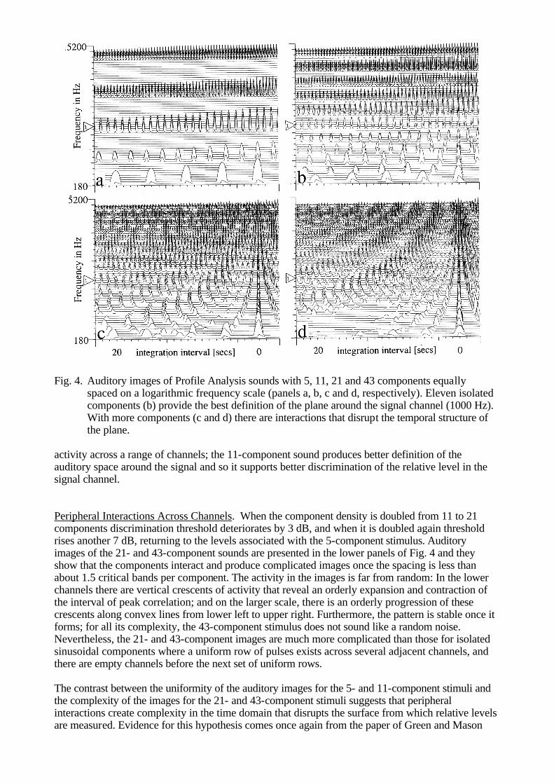
dominance in concurrent vowels as a function of stimulus duration and found an interesting contrast. One glottal period of a pair of vowels is sufficient to identify the dominant vowel accurately, while performance on the non-dominant rises slowly from chance to an asymptotic value well below that achieved on the dominant vowel over the course of about eight glottal periods. PROFILE ANALYSIS Historically, models of auditory intensity discrimination have not involved comparison of information extracted from widely separated frequency channels. Typically, the stimulus was either a sine wave or a broadband noise and the listener was instructed to determine which of two intervals contained the more intense version of the stimulus. When measured as a function of level, ? I/I for noise is found to be independent of level (Weber's law); in contrast, ? I/I for a tone decreases as level increases (the 'near miss to Weber's law'). It was assumed that the listener measured some aspect of the level of the sound in the signal channel and compared the estimates from the two intervals to decide which was the more intense. Models of the process were primarily concerned with the statistics of the internal representations of level for tones and noise (see Green, 1988, for a review). Recently, a series of experiments has been performed which indicates that traditional intensity discrimination experiments are misleading with regard to intensity perception in everyday life. Under more normal circumstances where there is energy in a range of channels, it appears that the auditory system measures intensity differences by comparing the level in the target band with that in other frequency bands (Green, 1988). One of the early experiments is particularly instructive: Green and Mason (1985) asked listeners to judge the relative intensity of a 1000 Hz tone which was the central member of a set of 5, 11, 21 or 43 tones. They were distributed uniformly across the frequency region 200 to 5000 Hz on a logarithmic frequency scale and in the standard interval they all had the same amplitude. In the test interval, the amplitude of the 1000 Hz component was incremented, and varied over trials to determine intensity discrimination threshold. The overall level of the stimulus was chosen at random from a wide range of levels, for each interval of every trial, to encourage the listeners to base their judgements on relative level. Intensity discrimination threshold is defined as the size of a 1000-Hz component that has to be added to the 1000-Hz component of the standard to support discrimination in the 2IFC task. When 6 extra sinusoids are added to the 5-component sound to produce the 11-component sound, intensity discrimination threshold drops by almost 10 dB. The authors argue that the extra components add useful definition to the internal spectrum, or Profile, of the sound and so assist measurement of the relative level of the 1000-Hz component. The phenomenon is very robust. As long as the components in the flanking bands are within 10 dB of the level in the signal channel, they serve to define the profile (Green and Kidd, 1983); furthermore, the level can vary across the flanking bands (Kidd, Mason and Green, 1986). Auditory images of stimuli with 5, 11, 21 and 43 components are shown in Fig. 4; in each case, there is a small increment in the 1000 Hz component which appears in the centre of the panel. The level is such as to be below threshold in the 5-component condition and above threshold in the 11-component condition. The auditory image of the five-component sound reveals five regular streams of pulses, each of which is the canonical pattern for a single sinusoid (Fig 4a). Similarly, the image of the 11-component sound reveals 11 sinusoidal sub-images (Fig 4b). The level of the components in panel b is lower than that in panel a because the model includes suppression and as the density of components increases, so the mutual suppression increases. However, aside from this global effect, there is essentially no interaction across channels. This supports Green's (1988) contention that the components are isolated and measurement of relative intensity must involve comparison of

Fig. 4. Auditory images of Profile Analysis sounds with 5, 11, 21 and 43 components equally

spaced on a logarithmic frequency scale (panels a, b, c and d, respectively). Eleven isolated components (b) provide the best definition of the plane around the signal channel (1000 Hz). With more components (c and d) there are interactions that disrupt the temporal structure of the plane.

activity across a range of channels; the 11-component sound produces better definition of the auditory space around the signal and so it supports better discrimination of the relative level in the signal channel. Peripheral Interactions Across Channels. When the component density is doubled from 11 to 21 components discrimination threshold deteriorates by 3 dB, and when it is doubled again threshold rises another 7 dB, returning to the levels associated with the 5-component stimulus. Auditory images of the 21- and 43-component sounds are presented in the lower panels of Fig. 4 and they show that the components interact and produce complicated images once the spacing is less than about 1.5 critical bands per component. The activity in the images is far from random: In the lower channels there are vertical crescents of activity that reveal an orderly expansion and contraction of the interval of peak correlation; and on the larger scale, there is an orderly progression of these crescents along convex lines from lower left to upper right. Furthermore, the pattern is stable once it forms; for all its complexity, the 43-component stimulus does not sound like a random noise. Nevertheless, the 21- and 43-component images are much more complicated than those for isolated sinusoidal components where a uniform row of pulses exists across several adjacent channels, and there are empty channels before the next set of uniform rows. The contrast between the uniformity of the auditory images for the 5- and 11-component stimuli and the complexity of the images for the 21- and 43-component stimuli suggests that peripheral interactions create complexity in the time domain that disrupts the surface from which relative levels are measured. Evidence for this hypothesis comes once again from the paper of Green and Mason

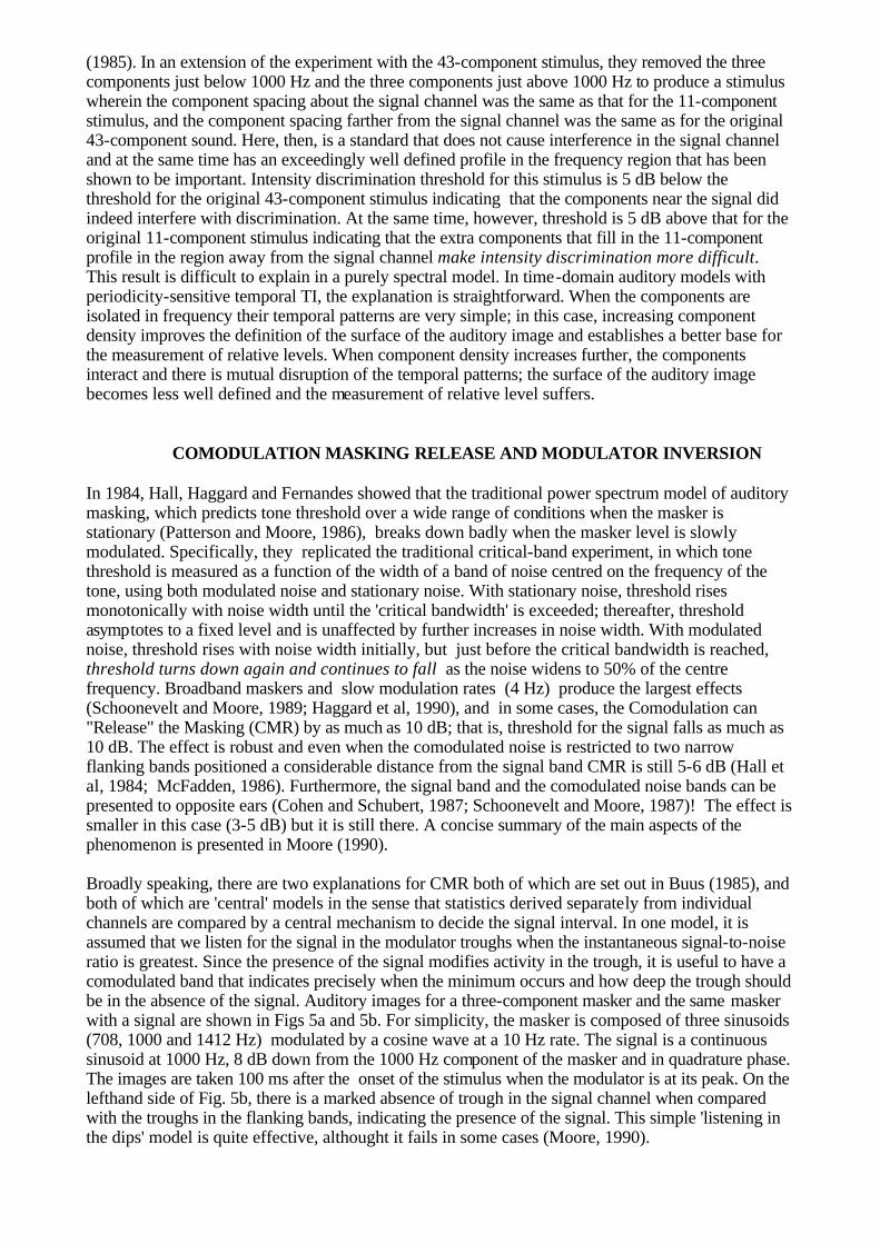
(1985). In an extension of the experiment with the 43-component stimulus, they removed the three components just below 1000 Hz and the three components just above 1000 Hz to produce a stimulus wherein the component spacing about the signal channel was the same as that for the 11-component stimulus, and the component spacing farther from the signal channel was the same as for the original 43-component sound. Here, then, is a standard that does not cause interference in the signal channel and at the same time has an exceedingly well defined profile in the frequency region that has been shown to be important. Intensity discrimination threshold for this stimulus is 5 dB below the threshold for the original 43-component stimulus indicating that the components near the signal did indeed interfere with discrimination. At the same time, however, threshold is 5 dB above that for the original 11-component stimulus indicating that the extra components that fill in the 11-component profile in the region away from the signal channel make intensity discrimination more difficult. This result is difficult to explain in a purely spectral model. In time-domain auditory models with periodicity-sensitive temporal TI, the explanation is straightforward. When the components are isolated in frequency their temporal patterns are very simple; in this case, increasing component density improves the definition of the surface of the auditory image and establishes a better base for the measurement of relative levels. When component density increases further, the components interact and there is mutual disruption of the temporal patterns; the surface of the auditory image becomes less well defined and the measurement of relative level suffers. COMODULATION MASKING RELEASE AND MODULATOR INVERSION In 1984, Hall, Haggard and Fernandes showed that the traditional power spectrum model of auditory masking, which predicts tone threshold over a wide range of conditions when the masker is stationary (Patterson and Moore, 1986), breaks down badly when the masker level is slowly modulated. Specifically, they replicated the traditional critical-band experiment, in which tone threshold is measured as a function of the width of a band of noise centred on the frequency of the tone, using both modulated noise and stationary noise. With stationary noise, threshold rises monotonically with noise width until the 'critical bandwidth' is exceeded; thereafter, threshold asymptotes to a fixed level and is unaffected by further increases in noise width. With modulated noise, threshold rises with noise width initially, but just before the critical bandwidth is reached, threshold turns down again and continues to fall as the noise widens to 50% of the centre frequency. Broadband maskers and slow modulation rates (4 Hz) produce the largest effects (Schoonevelt and Moore, 1989; Haggard et al, 1990), and in some cases, the Comodulation can "Release" the Masking (CMR) by as much as 10 dB; that is, threshold for the signal falls as much as 10 dB. The effect is robust and even when the comodulated noise is restricted to two narrow flanking bands positioned a considerable distance from the signal band CMR is still 5-6 dB (Hall et al, 1984; McFadden, 1986). Furthermore, the signal band and the comodulated noise bands can be presented to opposite ears (Cohen and Schubert, 1987; Schoonevelt and Moore, 1987)! The effect is smaller in this case (3-5 dB) but it is still there. A concise summary of the main aspects of the phenomenon is presented in Moore (1990). Broadly speaking, there are two explanations for CMR both of which are set out in Buus (1985), and both of which are 'central' models in the sense that statistics derived separately from individual channels are compared by a central mechanism to decide the signal interval. In one model, it is assumed that we listen for the signal in the modulator troughs when the instantaneous signal-to-noise ratio is greatest. Since the presence of the signal modifies activity in the trough, it is useful to have a comodulated band that indicates precisely when the minimum occurs and how deep the trough should be in the absence of the signal. Auditory images for a three-component masker and the same masker with a signal are shown in Figs 5a and 5b. For simplicity, the masker is composed of three sinusoids (708, 1000 and 1412 Hz) modulated by a cosine wave at a 10 Hz rate. The signal is a continuous sinusoid at 1000 Hz, 8 dB down from the 1000 Hz component of the masker and in quadrature phase. The images are taken 100 ms after the onset of the stimulus when the modulator is at its peak. On the lefthand side of Fig. 5b, there is a marked absence of trough in the signal channel when compared with the troughs in the flanking bands, indicating the presence of the signal. This simple 'listening in the dips' model is quite effective, althought it fails in some cases (Moore, 1990).

The alternative model focuses on comparisons of the envelopes observed in different channels. In the standard condition (Fig 5a), all of the channels have the same envelope. In the signal condition (Fig 5b), comparisons reveal that one channel has a different envelope with a filled trough. CMR persists when the flanking-band levels are up to 10 dB different from that of the signal band (Schoonevelt and Moore, 1987), which indicates that it is the envelope shape rather than the absolute peak-to-trough level that is compared across channels. With this modification the 'envelope comparison' model also works well. Attempts to discriminate between these central

Fig. 5. Auditory images of 3-component CMR sounds (708, 1000 and 1412 Hz) modulated at

a 10 Hz rate. The images are taken when there is a trough in the signal-channel modulator. The flanking-band modulator is identical to the signal-band modulator in (a) and (b); the signal is present in (b). The flanking-band modulator is inverted in (c) and (d); the signal is present in (d) but suppression from the flanking-band modulator peaks has reduced its level considerably.

CMR models experimentally are proceeding but as yet the results are inconclusive. It is perhaps more interesting at this point to turn briefly to some data that indicate that peripheral processes may also be involved in CMR. Modulator Inversion and Peripheral Interactions. Consider the situation that arises when the modulator waveform is inverted in the signal channel so that modulation troughs in the signal channel occur at the same time as modulation peaks in the flanking bands. It would seem reasonable to assume that a central mechanism that can use flanking-band modulation troughs to predict signal-band modulator troughs, could also use flanking-band modulator peaks to predict signal-band troughs, and thus reasonable to predict that inverting the modulator would have little effect on the CMR. The experiment has been performed by Moore, Glasberg and Schoonevelt (1990); the inversion of the modulator eliminates the CMR. The result is difficult to explain in a central model and suggests that peripheral suppression may be involved. The CMR example presented in the upper

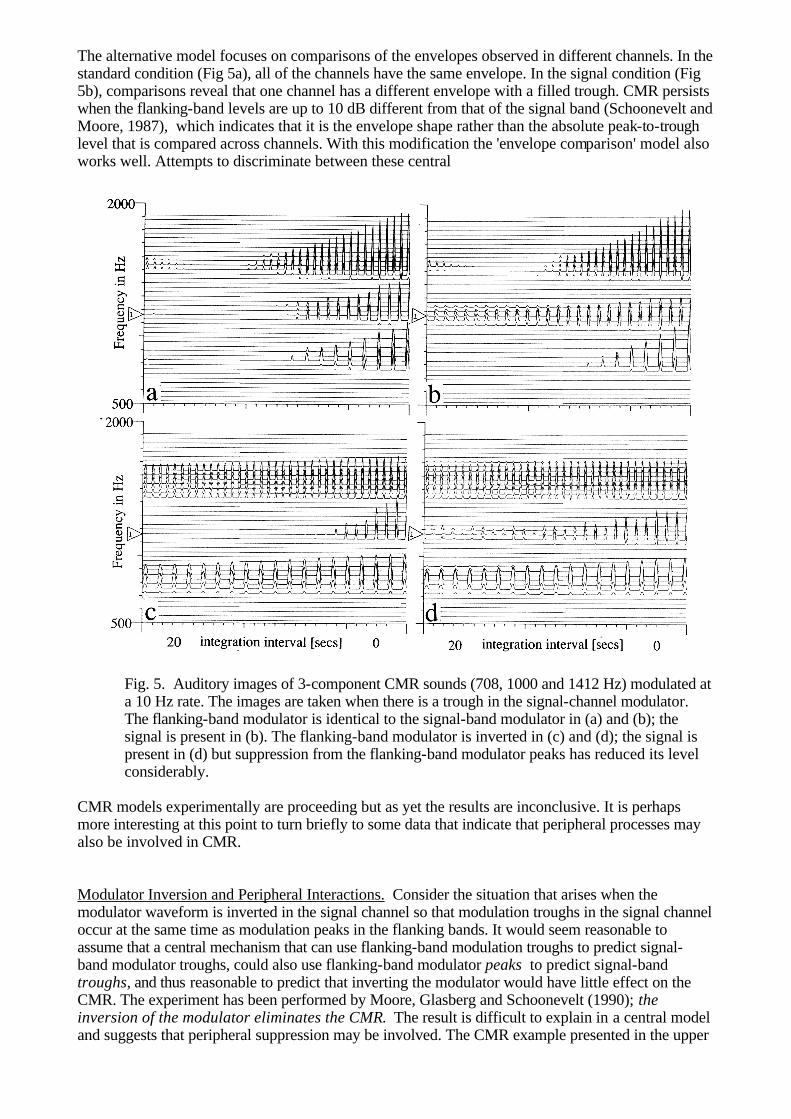
row of Fig. 5 is extended in the lower row where the modulator in the signal channel is inverted. The auditory images in the lower row are taken 50 ms farther along in the stimulus when the next signal-band trough occurs. At this point in time, the flanking-band modulators are at their maximum and suppressor activity flows from them across to the signal band. As a result, the signal in Fig. 5d is smaller than it is in Fig. 5b, and if the system is non-linear, the reduction could well make evaluation of the instantaneous signal-to-noise ratio in the trough more difficult. It is also the case, although it is not shown in the figure, that the modulation peak in the signal band is a little greater when the modulator is inverted because the flanking bands are at a minimum at this time and so there is a 'release from mutual suppression'. In summary, the cross-channel peripheral effects revealed in Fig. 5 suggest that the explanation of CMR will be even more complicated than indicated by the original central models. FIGURE AND GROUND IN THE AUDITORY IMAGE Periodicity-sensitive TI simplifies the representation of transients by phase aligning the channels and restricting the region of the representation where they may appear. It simplifies the representation of periodic sounds by phase aligning them and converting the repeating pattern that such sounds produce in the auditory nerve into a stabilised rectangular grid tied to the trigger-point vertical. It also enhances the contrast of the periodic pattern relative to that in the auditory nerve. At the same time, in the region away from the trigger point, periodicity-sensitive TI reduces the contrast of the representation of noise, relative to that in the auditory nerve. As a result, when we generate a real-time display of the auditory images of natural sounds, the transient and periodic components of the sounds often appear as solid objects in front of a shimmering background produced by attendant noise. The components of the auditory figures that arise in the individual channels of the auditory image are highly restricted in form. This is a direct consequence of the narrowband filtering imposed by the cochlea and it suggests that if we place some broad restrictions on the class of events considered to be figures, it might be possible to characterise the forms with simple functions and a small number of parameters. Briefly, the process would involve identifying figure components in individual channels and segregating channels with figure components that are vertically aligned and related. In this way we might begin the process of pattern recognition and provide an auditory representation with a dramatically reduced data rate which nevertheless preserves the figure information essential for recognising the sound source. The elements of this process are sketched in this final section in an attempt to reassure those interested in auditory models as preprocessors for auditory scene analysis, speech recognition or music, that peripheral auditory modelling will not involve an endless expansion of the data rate and an endless progression of new modules before the pattern recognition begins. Pulselets and Tonelets The vast majority of the pulses that appear in the NAP are the sharpened remains of the upper half-cycle of a filtered wave. They are like the tips of elongated, inverted parabolas and would be well approximated by this or any of a number of other simple functions. Transients and periodic sounds generate two-dimensional sets of these pulses that are highly regular, and periodicity-sensitive TI preserves the relationship in these shapes. Examples of figure components from the pulse train and click in Fig. 1c and 1d are presented in Fig. 6a and 6b, respectively. The examples are from channels centred near 1000, 2000 and 3000 Hz. The components in Fig. 6b are obviously filter impulse responses as they appear in the auditory image after feature enhancement and alignment. Each channel contains a set of regularly spaced pulses whose level decreases with time. Across channels, these figure components differ chiefly in the pulse spacing and the rate at which pulse level decreases, as indicated by the sloping lines drawn across the tops of the pulses. These are properties of the peripheral system that we could expect a central figure recognition system to know. Since a vertically-aligned set of these figure components indicates the presence of an acoustic pulse (Fig. 1d), the individual components might be referred to as 'pulselets'. The upper channels in Fig. 6a show that the upper portion of the auditory figure of a pulse train is a two-dimensional array of pulselets, which decay regularly in level from right to left across the image. The pulselets away from

the trigger point specify the period of the pulse train, the degree of periodicity, and whether the period is increasing or decreasing. The bottom channel in Fig. 6a is centred near the eighth harmonic of the pulse train and it shows that the impulse responses overlap for partially resolved harmonics. There is a further flattening of the slope of the peaks which continues as the centre frequency decreases and eventually, the slope becomes slightly negative as all of pulses become part of one large, extended figure component. Since a set of these extended components indicates the presence of a resolved sinusoid (Figs 4a and 4b), the individual components might be referred to as 'tonelets'. The auditory figures that appear in the examples of this paper are largely composed of pulselets and tonelets. The upper formants of the vowels in Fig. 3 are sets of pulselets which have steep slopes on the flanks of the formant and shallower slopes in the centre. The low formants are composed of sets of tonelets; the temporal harmonic relationships reveal which sets of tonelets come from the same source. The auditory images of the 5- and 11-component PA stimuli are

Fig. 6. Figure components that appear in three channels of the auditory image of a pulse train (a) and

a click (b). The parameters of these figure components might provide an efficient code for summarising peripheral auditory activity.

entirely composed of tonelets. It is assumed that the temporal uniformity of tonelets helps minimise the variability of the 5- and 11-component 'profiles' and so aids the measurement of relative level in the signal channel. The auditory images of the 21- and 43-component PA stimuli are composed neither of tonelets nor pulselets, and it is assumed that the temporal variability, or the lack of recognisable figure components, makes the measurement of relative level more difficult in the signal channel. The CMR stimuli in this paper are entirely composed of tonelets and so add little to this discussion. In any given channel, the activity in the region of the trigger point is a good guide to the form of the activity in the remainder of the auditory image. If the pulses are regularly spaced and nearly equal in height, a tonelet is indicated. If the pulses fall off rapidly and the pattern is strongly asymmetric a pulselet is indicated, and a check for other pulselets should be initiated to determine if the sound is periodic. More complicated patterns of broken or superimposed figure components would require more analysis and, as in the case of noise, might reveal no discernible pattern. Both the pulselets and the tonelets can be summarised by the height of the largest pulse, the slope of a line through the pulse peaks and the spacing of the pulses. Multiple pulselets occur in a channel when the sound is periodic but that is a minor complication. These, or similar, parameters may well provide a summary of auditory figure components that preserves the essential information while at the same time reducing the data rate, and so provides an efficient peripheral output code on which to base figure/ground segregation and figure recognition processes.

ACKNOWLEDGEMENTS The authors would like to thank Dave Green for helpful discussions concerning Profile Analysis and Brian Moore for helpful discussions concerning CMR and an earlier draft of the paper. The work presented in this paper was supported by the MRC and grants from Esprit BRA (project ACTS, 3207) and MOD PE (project AAM HAP, 2239). REFERENCES Aertsen, A. M. J. H. and P. I. M. Johannesma (1980). Spectro-temporal receptive fields of auditory neurons

in the grassfrog. I. Characterisation of tonal and natural stimuli. Biol. Cybern., 38, 223-234. Assman, P. F. and Q. Summerfield (1990). Modelling the perception of concurrent vowels: Vowels with

different fundamental frequencies, J. Acoust. Soc. Am., 88, 680-697. Boer, E. de and H. R. de Jongh (1978). On cochlear encoding: potentialities and limitations of the reverse-

correlation technique, J. Acoust. Soc. Am., 63, 115-135. Bregman, A.S. (1990). Auditory scene analysis. MIT Press, Cambridge MA. Buus, S. (1985). Release from masking caused by envelope fluctuations. J. Acoust. Soc. Am., 78, 1958-1965. Chalikia, M. H. and A. S. Bregman (1989). The perceptual segregation of simultaneous auditory signals: Pulse

train segregation, Perception and Psychophysics, 46, 487-496. Cohen, M. F. and E. D. Schubert (1987). Influence of place synchrony on detection of a sinusoid. J. Acoust.

Soc. Am., 81, 452-458. Glasberg, B. R. and B. C. J. Moore (1990). Derivation of auditory filter shapes from notched-noise data.

Hearing Research, 47, 103-138. Green, D. M. (1988). Profile Analysis: auditory intensity discrimination, Oxford University Press, New York. Green, D. M. and G. Kidd Jr. (1983). Further studies of auditory profile analysis. J. Acoust. Soc. Am., 73,

1260-1265. Green, D. M. and C. R. Mason, (1985). Auditory profile analysis: Frequency, phase, and Weber's law. J.

Acoust. Soc. Am., 77, 1155-1161. Greenwood, D. D. (1990). A cochlear frequency-position function for several species - 29 years later. J.

Acoust. Soc. Am., 87, 2592-2605. Haggard, M. P., J. L. Hall, III, and J.H. Grose (1990). Comodulation masking release as a function of

bandwidth and test frequency. J. Acoust. Soc. Am., 88, 113-118. Hall, J. W., M. P. Haggard and M. A. Fernandes (1984). Detection in noise by spectro-temporal pattern

analysis. J. Acoust. Soc. Am., 76, 50-56. Holdsworth, J. (1990). Two-Dimensional adaptive thresholding. Annex 4 of APU AAM-HAP Report 1. Kidd, G. Jr., C. R. Mason and D. M. Green (1986). Auditory profile analysis of irregular sound spectra. J.

Acoust. Soc. Am., 79, 1045-1053. Licklider, J. C. R. (1951). A duplex theory of pitch perception, Experientia, 7, 128-133. Reprinted in E. D.

Schubert (ed.), Psychological Acoustics. Stroudsburg, P. A., Dowden, Hutchinson and Ross Inc. (1979). Lyon, R.F. (1982). A computational model of filtering, detection, and compression in the cochlea. In: Proc.

IEEE Int. Conf. Acoust., Speech Signal Processing. Paris, France. May 1982. Lyon, R.F. (1984). Computational models of neural auditory processing. In: Proc. IEEE Int. Conf. Acoust.,

Speech Signal Processing. San Diego, CA. March 1984. McFadden, D. (1986). Comodulation masking release: Effects of varying the level, duration and time delay of

the cue band. J. Acoust. Soc. Am., 80, 1658-1667. McKeown, D. (1990). The time course of auditory segregation of simultaneous vowels. J. Acoust. Soc. Am.,

88, S27. Meddis, R. and M. J. Hewitt (1991a). Virtual pitch and phase sensitivity of a computer model of the auditory

periphery: I pitch identification. submitted to J. Acoust. Soc. Am. Meddis, R. and M. J. Hewitt (1991b). Modelling the perception of concurrent vowels with different

fundamental frequencies, submitted to J. Acoust. Soc. Am. Moore, B.C.J. (1990). Comodulation Masking Release: spectro-temporal pattern analysis in hearing. Br. J.

Audiology, 24, 131-137. Moore, B.C.J., B.R. Glasberg and G.P. Schoonevelt (1990). Across-channel masking and comodulation

masking release. J. Acoust. Soc. Am., 87, 1683-94. Patterson, R. D. (1987). A pulse ribbon model of monaural phase perception. J. Acoust. Soc. Am., 82, 1560-

1586. Patterson, R. D., J. Holdsworth, I. Nimmo-Smith and P. Rice (1988). SVOS Final Report: The Auditory

Filterbank. APU report 2341. Patterson, R.D. and J. Holdsworth (1991). A functional model of neural activity patterns and auditory images.

In: Advances in Speech, Hearing and Language Processing , (W. A. Ainsworth, ed.), Vol 3. JAI Press, London. (in press). [This chapter eventually appeared in 1996.]

Patterson, R. D. and B. C. J. Moore (1986). Auditory filters and excitation patterns as representations of frequency resolution. In: Frequency Selectivity in Hearing (B. C. J. Moore, ed.), pp. 123-177. Academic Press Limited, London.

Scheffers, M. T. M. (1983a). Sifting vowels: Auditory pitch analysis and sound segregation. Unpublished Ph.D. thesis, University of Groningen, The Netherlands.

Scheffers, M. T. M. (1983b). Simulation of the auditory analysis of pitch: An elaboration on the DWS meter. J. Acoust. Soc. Am., 74, 1716-1725.

Schooneveldt, G. P. and B. C. J. Moore (1987). Comodulation masking release (CMR): Effects of signal frequency, flanking-band frequency, masker band-width, flanking-band level, and monotic versus dichotic presentation of the flanking band. J. Acoust. Soc. Am., 82, 1944-1956.

Schooneveldt, G. P. and B. C. J. Moore (1989). Comodulation masking release for various monaural and binaural combinations of the signal, on-frequency and flanking bands. J. Acoust. Soc. Am., 85, 262-272.

For reprints email roy.patterson@mrc-cbu.cam.ac.uk Roy D. Patterson, Centre for the Neural Basis of Hearing Physiology Department, University of Cambridge Downing Street, Cambridge, CB2 3EG http://www.mrc-cbu.cam.ac.uk/~roy.patterson http://www.mrc-cbu.cam.ac.uk/cnbh