76
Complexities of Order-Related Formal Language E x t e n s i o n s q q e q x q n q s q w Martin Berglund Ume˚ a 2014 Department of Computing Science

Complexities of Order-RelatedFormal Language Extensions
q
qe qx qn qs
qw
Martin Berglund
Umea 2014Department of Computing Science

Complexities of Order-RelatedFormal Language Extensions
Martin Berglund
PHD THESIS, MAY 2014DEPARTMENT OF COMPUTING SCIENCE
UMEA UNIVERSITYSWEDEN
Department of Computing ScienceUmea UniversitySE-901 87 Umea, Sweden
Copyright c© 2014 by authors
ISBN 978-91-7601-047-1ISSN 0348-0542UMINF 14.13
Cover photo by Tc Morgan (used under Creative Commons license BY-NC-SA 2.0).Printed by Print & Media, Umea University, 2014.

Abstract
The work presented in this thesis discusses various formal language formalisms thatextend classical formalisms like regular expressions and context-free grammars withadditional abilities, most relating to order. This is done while focusing on the im-pact these extensions have on the efficiency of parsing the languages generated. Thatis, rather than taking a step up on the Chomsky hierarchy to the context-sensitivelanguages, which makes parsing very difficult, a smaller step is taken, adding somemechanisms which permit interesting spatial (in)dependencies to be modeled.
The most immediate example is shuffle formalisms, where existing language for-malisms are extended by introducing operators which generate arbitrary interleavingsof argument languages. For example, introducing a shuffle operator to the regular ex-pressions does not make it possible to recognize context-free languages like anbn, butit does capture some non-context-free languages like the language of all strings con-taining the same number of as, bs and cs. The impact these additions have on parsinghas many facets. Other than shuffle operators we also consider formalisms enforcingrepeating substrings, formalisms moving substrings around, and formalisms that re-strict which substrings may be concatenated. The formalisms studied here all have anumber of properties in common.
1. They are closely related to existing regular and context-free formalisms. Theyoperate in a step-wise fashion, deriving strings by sequences of rule applicationsof individually limited power.
2. Each step generates a constant number of symbols and does not modify partsthat have already been generated. That is, strings are built in an additive fashionthat does not explode in size (in contrast to e.g. Lindenmayer systems). Alllanguages here will have a semi-linear Parikh image.
3. They feature some interesting characteristic involving order or other spatial con-straints. In the example of the shuffle multiple derivations are in a sense inter-spersed in a way that each is unaware of.
4. All of the formalisms are intended to be limited enough to make an efficientparsing algorithm at least for some cases a reasonable goal.
This thesis will give intuitive explanations of a number of formalisms fulfilling theserequirements, and will sketch some results relating to the parsing problem for them.This should all be viewed as preparation for the more complete results and explana-tions featured in the papers given in the appendices.
iii

iv

Sammanfattning
Denna avhandling diskuterar utokningar av klassiska formalismer inom formella sprak,till exempel reguljara uttryck och kontextfria grammatiker. Utokningarna handlar paett eller annat satt om ordning, och ett sarskilt fokus ligger pa att gora utokningarnapa ett satt som dels har intressanta spatiala/ordningsrelaterade effekter och som delsbevarar den effektiva parsningen som ar mojlig for de ursprungliga klassiska forma-lismerna. Detta star i kontrast till att ta det storre steget upp i Chomsky-hierarkin tillde kontextkansliga spraken, vilket medfor ett svart parsningsproblem.
Ett omedelbart exempel pa en sadan utokning ar s.k. shuffle-formalismer. Des-sa utokar existerande formalismer genom att introducera operatorer som godtyckligtsammanflatar strangar fran argumentsprak. Om shuffle-operator introduceras till dereguljara uttrycken ger det inte formagan att kanna igen t.ex. det kontextfria spraketanbn, men det fangar istallet vissa sprak som inte ar kontextfria, till exempel spraketsom bestar av alla strangar som innehaller lika manga a:n, b:n och c:n. Sattet pa vil-ket dessa utokningar paverkar parsningsproblemet ar mangfacetterat. Utover dessashuffle-operatorer tas ocksa formalismer dar delstrangar kan upprepas, formalismerdar delstrangar flyttas runt, och formalismer som begransar hur delstrangar far konka-teneras upp. Formalismerna som tas upp har har dock vissa egenskaper gemensamma.
1. De ar nara beslaktade med de klassiska reguljara och kontextfria formalismerna.De arbetar stegvis, och konstruerar strangar genom successiva applikationer avindividuellt enkla regler.
2. Varje steg genererar ett konstant antal symboler och modifierar inte det somredan genererats. Det vill saga, strangar byggs additivt och langden pa dem kaninte explodera (i kontrast till t.ex. Lindenmayer-system). Alla sprak som tar uppkommer att ha en semi-linjar Parikh-avbildning.
3. De har nagon instressant spatial/ordningsrelaterad egenskap. Exempelvis sattetpa vilket shuffle-operatorer sammanflatar annars oberoende deriveringar.
4. Alla formalismera ar tankta att vara begransade nog att det ar resonabelt att haeffektiv parsning som mal.
Denna avhandling kommer att ge intuitiva forklaring av ett antal formalismer somuppfyller ovanstaende krav, och kommer att skissa en blandning av resultat relateradetill parsningsproblemet for dem. Detta bor ses som forberedande infor lasning av demer djupgaende och komplexa resultaten och forklaringarna i de artiklar som finnsinkluderade som appendix.
v

vi

Preface
This thesis consists of an introduction which discusses some different language for-malisms in the field of formal languages, touches upon some of their properties andtheir relations to each other, and gives a short overview of relevant research. In the ap-pendix the following six articles, relating to the subjects discussed in the introduction,are included.
Paper I Martin Berglund, Henrik Bjorklund, and Johanna Bjorklund. Shuffled lan-guages – representation and recognition. Theoretical Computer Science,489-490:1–20, 2013.
Paper II Martin Berglund, Henrik Bjorklund, and Frank Drewes. On the parameter-ized complexity of Linear Context-Free Rewriting Systems. In Proceed-ings of the 13th Meeting on the Mathematics of Language (MoL 13), pages21–29, Sofia, Bulgaria, August 2013. Association for Computational Lin-guistics.
Paper III Martin Berglund, Henrik Bjorklund, Frank Drewes, Brink van der Merwe,and Bruce Watson. Cuts in regular expressions. In Marie-Pierre Beal andOlivier Carton, editors, Proceeding of the 17th International Conferenceon Developments in Language Theory (DLT 2013), pages 70–81, 2013.
Paper IV Martin Berglund, Frank Drewes, and Brink van der Merwe. Analyzingcatatrophic backtracking behavior in practical regular expression match-ing. Submitted to the 14th International Conference on Automata andFormal Languages (AFL 2014), 2014.
Paper V Martin Berglund. Characterizing non-regularity. Technical Report UMINF14.12, Computing Science, Umea University, http://www8.cs.umu.se/research/uminf/, 2014. In collaboration with Henrik Bjorklundand Frank Drewes.
Paper VI Martin Berglund. Analyzing edit distance on trees: Tree swap distanceis intractable. In Jan Holub and Jan Zdarek, editors, Proceedings of thePrague Stringology Conference 2011, pages 59–73. Prague StringologyClub, Czech Technical University, 2011.
vii

viii

Acknowledgments
I must firstly thank my primary advisor, Frank Drewes, who made all this both pos-sible, enjoyable and inspiring. In much the same vein I thank my co-advisor, HenrikBjorklund, who knows many things and throws a good dinner party, as well as my un-official co-advisor Johanna Bjorklund, who organizes many things and makes peoplehave fun when they otherwise would not. I must also thank the rest of my universitycolleagues, in the Natural and Formal Languages Group (thanks to Niklas, Petter andSuna) and many others in many other places. A special thank you to all the supportand administrative staff at the department and university, who have helped me outwith countless things on countless occasions, a fact too easily forgotten. I also owe agreat debt to all my research collaborators outside of this university, including but notlimited to Brink van der Merwe and Bruce Watson. I thank those who have given meuseful research advice along the way, like Michael Minock and Stephen Hegner.
On the slightly less professional front I thank my family for their support, in par-ticular in offering places and moments of calm when things were hectic. I thank myfriends who have helped both distract from and inspire my work as appropriate, thanksto, among many others, Gustaf, Sandra, Josefin, Sigge, Marten, John, a Magnus ortwo, some Tommy, perhaps a Johan and a Maria, and many many more.
I wish to dedicate this work to the memory of Holger Berglund and Bertil Larsson,both of my grandfathers, who passed away during my studies leading up to this thesis.
ix

x

Contents
1 Introduction 11.1 Formal Languages 21.2 An Example Representation 3
1.2.1 Our Grammar Sketch 31.2.2 Generating Regular Languages 41.2.3 Regular Expressions as an Alternative 5
1.3 Computational Problems in Formal Languages 51.4 Outline of Introduction 7
2 Shuffle-Like Behaviors in Languages 92.1 The Binary Shuffle Operator 92.2 Sketching Grammars Capturing Shuffle 92.3 The Shuffle Closure 112.4 Shuffle Operators and the Regular Languages 122.5 Shuffle Expressions and Concurrent Finite State Automata 142.6 Overview of Relevant Literature 142.7 CFSA and Context-Free Languages 152.8 Membership Problems 16
2.8.1 The Membership Problems for Shuffle Expressions 172.8.2 The Membership Problems for General CFSA 17
2.9 Contributions In the Area of Shuffle 172.9.1 Definitions and Notation 172.9.2 Concurrent Finite State Automata 182.9.3 Properties of CFSA 192.9.4 Membership Testing CFSA 192.9.5 The rest of Paper I. 202.9.6 Language Class Impact of Shuffle 21
3 Synchronized Substrings in Languages 233.1 Sketching a Synchronized Substrings Formalism 23
3.1.1 The Graphical Intuition 233.1.2 Revisiting the Mapped Copies of Example 1.1 253.1.3 Grammars for the Mapped Copy Languages 253.1.4 Parsing for the Mapped Copy Languages 25
3.2 The Broader World of Mildly Context-Sensitive Languages 273.2.1 The Mildly Context-Sensitive Category 27
xi
3.2.2 The Mildly Context-Sensitive Classes 273.3 String-Generating Hyperedge Replacement Grammars 283.4 Deciding the Membership Problem 29
3.4.1 Deciding Non-Uniform Membership 293.4.2 Deciding Uniform Membership 313.4.3 On the Edge Between Non-Uniform and Uniform 32
3.5 Contributions in Fixed Parameter Analysis of Mildly Context-SensitiveLanguages 323.5.1 Preliminaries in Fixed Parameter Tractability 323.5.2 The Membership Problems of Paper II 33
4 Constraining Language Concatenation 354.1 The Binary Cut Operator 354.2 Reasoning About the Cut 364.3 Real-World Cut-Like Behavior 364.4 Regular Expressions With Cut Operators Remain Regular 37
4.4.1 Constructing Regular Grammars for Cut Expressions 374.4.2 Potential Exponential Blow-Up in the Construction 38
4.5 The Iterated Cut 404.6 Regular Expression Extensions, Impact and Reality 41
4.6.1 Lifting Operators to the Sets 414.6.2 An Aside: Regular Expression Matching In Common Software 424.6.3 Real-World Cut-Like Operators 424.6.4 Exploring Real-World Regular Expression Matchers 43
4.7 The Membership Problem for Cut Expressions 44
5 Block Movement Reordering 475.1 String Edit Distance 475.2 A Look at Error-Dilating a Language 475.3 Adding Reordering 49
5.3.1 Reordering Through Symbol Swaps 495.3.2 Derivation-Level Reordering 495.3.3 Tree Edit Distance 50
5.4 Analyzing the Reordering Error Measure 50
6 Summary and Loose Ends 536.1 Open Questions and Future Directions 53
6.1.1 Shuffle Questions 536.1.2 Synchronized Substrings Questions 546.1.3 Regular Expression Questions 546.1.4 Other Questions 55
6.2 Conclusion 55
Paper I 63
Paper II 103
xii

Paper III 115
Paper IV 129
Paper V 149
Paper VI 161
xiii

xiv
CHAPTER 1
Introduction
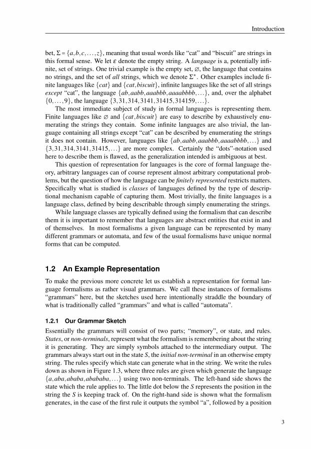
This thesis studies extensions of some classical formal languages formalisms, notablyfor the regular and context-free languages. The extensions center primarily around ad-ditions of operations or mechanism that constrain or loosen order, with a special focuson parsing in the presence of such ordering loosening or constraints. This statementis, of course, quite vague. The extensions take such a form that they modify the wayin which a grammar or automaton generates a string. “Order” here refers to a spatialview of this generation.
Very informally, imagine a person with finite memory (a natural assumption) whois tasked to write down certain types of strings of symbols on paper. The ways inwhich he or she is allowed to move around the paper will impact the types of stringsthey can write. If they are required to start at the left (i.e., start with the first, leftmost,symbol) and work their way through the string in a left-to-right fashion they can easilywrite the string abcabcabc . . ., but the strings {ab,aabb,aaabbb, . . .} (i.e. as followedby an equal number of bs) require them to remember the number of as written if it isdone in a left-to-right fashion, which is arbitrarily much information to remember. Ifthe person is permitted to keep track of the middle of the string, adding symbols onthe right and left side simultaneously, they can easily write strings of the second typeby simply in each step writing one a and one b, never having to remember how manysteps have been made. The first variant, where the person has to work left-to-rightand cannot remember arbitrarily much is an informal description of finite automata, acharacterization of the very important class of regular languages. The case where theperson keeps track of the middle and writes on both the left and the right correspondsto the class of linear context-free languages, another very classical concept. From thisperspective it is easy to imagine additional extensions of the formalisms, a notableexample is that the writer may remember multiple positions, and add symbols to theminterchangeably, which corresponds to a more complex language class.
Among the variety of formalisms one can imagine that modify the way in whichgeneration happens it is important to remain true to the spirit of classical mechanisms.This tends to return to the idea that only finite memory is required when viewed fromthe correct perspective. Consider for example the following trivial formalism.
Example 1.1 (Mappings of copy-languages) Given two mappings σ1,σ2 from {a,b}to arbitrary strings and a string w decide whether there exist some α1, . . . ,αn ∈ {a,b}such that σ1(α1)⋯σ1(αn) ⋅σ2(α1)⋯σ2(αn) =w. ◇
1

Chapter 1
This particular example is simplified quite a bit, but there are popular formalisms ex-hibiting this exact behavior, where some underlying “decision” is made in one deriva-tion step, and the result gets reflected in multiple (but normally constant number of)places in the output string. The mapping may make it difficult to actually recognizethe decision after the fact, but the problem is very related to parsing for some languageclasses with similar spatial dependencies.
Not all formalisms are concerned with instilling this extra level of order on thestring, we also consider cases where separate “underlying decisions” may become in-tertwined or otherwise not get spatially separated in the way we are used to. Considerthe following example of a fairly important real-world problem where difficulties arisefrom insufficient order.
Example 1.2 (Parallel program verification) Let P be a computer program whichwhen run produces some output string. Assume we have a context-free grammar Gwhich is such that if a string w can be output by a correct run of P then w can bederived in G. Then, whenever P produces output that is not accepted by G we knowthat P is not functioning properly.
Now run n copies of the program P, in parallel, all producing output simultane-ously into the same string w. In w the outputs of the different instances of P will bearbitrarily interleaved. Now we wish to use G to determine whether this w is consistentwith n copies of P running correctly. ◇The lack of order makes this problem difficult, to answer the question we need tosomehow track how single decisions in single instances of the program may have beenspread out across the resulting string. As these artifacts may be arbitrarily far apartthis problem becomes rather difficult, and the unfortunate reality is that the string wmay appear consistent despite a program failing to run in accordance with G, due tosome other part of the string masking the fault.
The cases in Example 1.1 and Example 1.2 are almost each others opposites, butare connected in that they are both possible to describe by a spatial dependence in thestrings. A simple block-wise dependence in Example 1.1, and an entirely scattereddependence in Example 1.2.
Earlier Work This work is deeply related to the preceding licentiate thesis [Ber12]by the same author. While this thesis is intended to replace this earlier work it may forsome readers be of interest to refer back to [Ber12] for further examples and explana-tions of many of the same concepts.
1.1 Formal Languages
Formal languages is a vast area of study, it covers both a lot of practical algorithmicwork with numerous application areas, as well as more theoretically founded mathe-matical study. The original subject of study in formal languages are string languages.These are concerned with sequences of symbols from a finite alphabet, which is usu-ally denoted Σ. Going forward we will usually simply assume that Σ is the latin alpha-
2
Introduction
bet, Σ = {a,b,c, . . . ,z}, meaning that usual words like “cat” and “biscuit” are strings inthis formal sense. We let ε denote the empty string. A language is a, potentially infi-nite, set of strings. One trivial example is the empty set, ∅, the language that containsno strings, and the set of all strings, which we denote Σ∗. Other examples include fi-nite languages like {cat} and {cat,biscuit}, infinite languages like the set of all stringsexcept “cat”, the language {ab,aabb,aaabbb,aaaabbbb, . . .}, and, over the alphabet{0, . . . ,9}, the language {3,31,314,3141,31415,314159, . . .}.
The most immediate subject of study in formal languages is representing them.Finite languages like ∅ and {cat,biscuit} are easy to describe by exhaustively enu-merating the strings they contain. Some infinite languages are also trivial, the lan-guage containing all strings except “cat” can be described by enumerating the stringsit does not contain. However, languages like {ab,aabb,aaabbb,aaaabbbb, . . .} and{3,31,314,3141,31415, . . .} are more complex. Certainly the “dots”-notation usedhere to describe them is flawed, as the generalization intended is ambiguous at best.
This question of representation for languages is the core of formal language the-ory, arbitrary languages can of course represent almost arbitrary computational prob-lems, but the question of how the language can be finitely represented restricts matters.Specifically what is studied is classes of languages defined by the type of descrip-tional mechanism capable of capturing them. Most trivially, the finite languages is alanguage class, defined by being describable through simply enumerating the strings.
While language classes are typically defined using the formalism that can describethem it is important to remember that languages are abstract entities that exist in andof themselves. In most formalisms a given language can be represented by manydifferent grammars or automata, and few of the usual formalisms have unique normalforms that can be computed.
1.2 An Example Representation
To make the previous more concrete let us establish a representation for formal lan-guage formalisms as rather visual grammars. We call these instances of formalisms“grammars” here, but the sketches used here intentionally straddle the boundary ofwhat is traditionally called “grammars” and what is called “automata”.
1.2.1 Our Grammar Sketch
Essentially the grammars will consist of two parts; “memory”, or state, and rules.States, or non-terminals, represent what the formalism is remembering about the stringit is generating. They are simply symbols attached to the intermediary output. Thegrammars always start out in the state S, the initial non-terminal in an otherwise emptystring. The rules specify which state can generate what in the string. We write the rulesdown as shown in Figure 1.3, where three rules are given which generate the language{a,aba,ababa,abababa, . . .} using two non-terminals. The left-hand side shows thestate which the rule applies to. The little dot below the S represents the position in thestring the S is keeping track of. On the right-hand side is shown what the formalismgenerates, in the case of the first rule it outputs the symbol “a”, followed by a position
3

Chapter 1
(●●)S
Ð→ (aa●●)A
(●●)A
Ð→ (bb●●)S
(●●)S
Ð→ (aa)Figure 1.3: A regular grammar generating the language {a,aba,ababa,abababa, . . .}using three rules. S is the initial non-terminal.
which is kept track of by the second non-terminal A. In effect S “remembers” thatthe next symbol should be an “a”, and the second non-terminal A remembers that thenext symbol should be a “b” (and we then go back to S. The third rule allows the Sto generate a final “a” and ending the generation by producing no new non-terminal.Since the first and third rule have the same left-hand side the abbreviation
(●●)S
Ð→ (aa●●)A
(aa)is sometimes used in place of writing both out in full. We write the generation ofstrings in the way shown in Figure 1.4, where a derivation is performed using thegrammar from Figure 1.3 to generate the string “ababa”. Notice that, as usual, none
(●●)S
Ô⇒ (aa●●)A
Ô⇒ (aabb●●)S
Ô⇒ (aabbaa●●)A
Ô⇒ (aabbaabb●●)S
Ô⇒ (aabbaabbaa)Figure 1.4: A derivation of the string “ababa” using the grammar Figure 1.3. Thederivation starts with the initial non-terminal S, applies the first rule, this produces thenon-terminal A, making the second rule the only possible one. This is then repeated,and finally the third rule is used to get rid of the non-terminal S entirely. As there is nomore state left the derivation is finished, and the string “ababa” has been generated.The dotted outline around non-terminals show which non-terminal is used in the nextrule application, but as there is only one to choose from in each step it is not veryinformative here.
of the intermediary strings are “generated”, all states must be gone before generationis finished. The black bullets, or “positions” act as the points of the string tracked byattached non-terminals. Their role will become slightly more complex later on.
1.2.2 Generating Regular Languages
A simple and important class of languages that we can generate with grammars of thetype we have sketched are the regular languages. Specifically the regular languagesare precisely the following.
Definition 1.5 (Regular Grammars) A grammar of the form sketched in Figure 1.3is regular if
4

Introduction
• It is finite.
• Each right-hand side contains zero or one symbol from Σ and zero or one non-terminal attached to the position (bullet).
• The position is to the right of the symbol if one exists.
Every regular language can be represented by a grammar of this form. ◇A grammar G then generates exactly the strings one can produce by starting from Sattached to the initial position, and then repeatedly picking a rule, and replacing aninstance of the non-terminal on the left-hand side of the rule (this is then only possibleif that non-terminal exists in the string) by the new substring on the right-hand side ofthe rule. If a point is reached where no non-terminal exists in the string the generatedstring w is in the language, denoted w ∈ L(G). That is, L(G) is a set consisting ofexactly these strings.
1.2.3 Regular Expressions as an Alternative
A regular expression is another way of expressing a language, which is equivalentto the description of a regular grammar in Definition 1.5, but which is often morecompact and convenient, as well as being very popular in practical use.
Definition 1.6 (Regular Expressions) A regular expression over the alphabet Σ is,inductively, the following. For each α ∈ Σ and regular expressions R and T :
• ε is a regular expression with L(ε) = {ε}.
• α is a regular expression with L(α) = {α}.
• R ⋅T is a regular expression with L(R ⋅T) = {wv ∣ w ∈ L(R),v ∈ L(T)} (i.e. theconcatenation of the strings in the languages of the subexpressions). We oftenwrite RT as an abbreviation.
• R ∣T is a regular expression, with L(R ∣T) = L(R)∪L(T).
• R∗ is a regular expression, with L(R∗) = {ε}∪{wv ∣ w ∈ L(R),v ∈ L(R∗)} in-ductively. That is, the concatenation of arbitrarily many strings from R. ◇
1.3 Computational Problems in Formal Languages
With formalisms for representing formal languages in hand it is time to consider thevarious questions that can be asked about them. An immediate example is the empti-ness problem; given a grammar G, does it generate the language ∅? Computing theanswer to this problem is easy for context-free languages1, but it is undecidable todetermine if a context-free language generates Σ∗, the language of all strings.
1 We have not defined the context-free languages properly, but all regular languages are context-free, andsome context-free languages are not regular, so it can serve as an unspecific more powerful example.
5
Chapter 1
Many problems also deal with languages themselves, being somewhat independentof representation. For example, given two context-free languages (i.e., two languagesthat can be generated by some context-free grammar) L and L′, is the language L∪L′also context-free? It, in fact, is, and given any context-free grammar for L and L′ agrammar for L∪L′ can easily be constructed. The same does not hold for the languageL∩L′, some context-free languages have an intersection that is not context-free. Theregular languages, however, as closed under intersection, so for all regular languagesL and L′ the language L∩L′ is regular as well, a fact we will make use of later.
It is important to remember that while grammars may determine languages thegrammar is not necessarily always in the most convenient form. Given a regulargrammar G it is easy to determine if it generates Σ∗, but it is hard to determine ifa context-free grammar generates Σ∗. However, context-free grammars can generateall the regular languages as well, but even if a context-free grammar generates a reg-ular language it is still hard to tell if it generates Σ∗ (in fact, as Σ∗ is regular this is apart of the general problem).
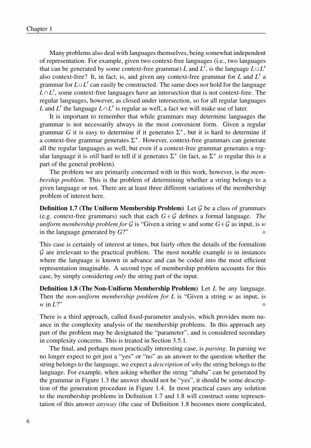
The problem we are primarily concerned with in this work, however, is the mem-bership problem. This is the problem of determining whether a string belongs to agiven language or not. There are at least three different variations of the membershipproblem of interest here.
Definition 1.7 (The Uniform Membership Problem) Let G be a class of grammars(e.g. context-free grammars) such that each G ∈ G defines a formal language. Theuniform membership problem for G is “Given a string w and some G ∈ G as input, is win the language generated by G?” ◇This case is certainly of interest at times, but fairly often the details of the formalismG are irrelevant to the practical problem. The most notable example is in instanceswhere the language is known in advance and can be coded into the most efficientrepresentation imaginable. A second type of membership problem accounts for thiscase, by simply considering only the string part of the input.
Definition 1.8 (The Non-Uniform Membership Problem) Let L be any language.Then the non-uniform membership problem for L is “Given a string w as input, isw in L?” ◇There is a third approach, called fixed-parameter analysis, which provides more nu-ance in the complexity analysis of the membership problems. In this approach anypart of the problem may be designated the “parameter”, and is considered secondaryin complexity concerns. This is treated in Section 3.5.1.
The final, and perhaps most practically interesting case, is parsing. In parsing weno longer expect to get just a “yes” or “no” as an answer to the question whether thestring belongs to the language, we expect a description of why the string belongs to thelanguage. For example, when asking whether the string “ababa” can be generated bythe grammar in Figure 1.3 the answer should not be “yes”, it should be some descrip-tion of the generation procedure in Figure 1.4. In most practical cases any solutionto the membership problems in Definition 1.7 and 1.8 will construct some represen-tation of this answer anyway (the case of Definition 1.8 becomes more complicated,
6
Introduction
however, as the internal representation of the language may be hard to practically de-cipher). Thanks to this fact this thesis will primarily refer to and work on membershipproblems, despite it being understood that parsing is the real goal.
1.4 Outline of Introduction
In the following chapters we will look at some formalisms that are of interest for thisthesis (and are studied in the papers included). We will start out using variations onthe informal notation demonstrated above (as in Figure 1.3), modifying it to illustratethe general idea of how the formalisms differ. More formalized, and deeper, mattersare then considered for each.
For the most part each chapter starts out with a self-contained informal introduc-tion, with a more formal treatment being undertaken at the end. This is intended tocater to multiple types of readers. A casual reader may be most interested in readingevery chapter only up until the section marked by a star, ☆, and then skipping to thenext. The non-starred portion of the introduction is self-contained. For a deeper treat-ment the entirety of the introduction may be read, but, of course, in the end most ofthe material is in the accompanying papers, and readers familiar with the area may bebest served only skimming the introduction in favor of proceeding to the papers.
Chapter 2 gives a light introduction to shuffle formalisms, which are related toExample 1.2, extending regular expressions with an operator that interleaves strings.This sets the scene for a short summary of the contents of Paper I, with some wordson Paper V in addition. Chapter 3 discusses synchronized substrings, similar to Ex-ample 1.1, going into a summary of Paper II. Chapter 4 discusses some extensions ofregular expressions, primarily dealing with the cut operator, which provides a morelimited string concatenation, but also giving an overview of some of the details of real-world matching engines. Papers III and IV are then discussed in brief in this context.Chapter 5 discusses distance measures on languages for handling errors. This yieldsa short discussion of grammar-instructed block movements, where substrings may bemoved around in the string depending on how they were generated by a grammar,leading into Paper VI. Finally, Chapter 6 provides a short summary.
7

Chapter 1
8

CHAPTER 2
Shuffle-Like Behaviors inLanguages
Shuffle in the title of this chapter refers to shuffling a deck of cards, specifically to theriffle shuffle, where the deck is separated into two halves, which are then interleaved.This idea, transferred to formal languages, is intended to capture situations such asthe one illustrated in Example 1.2, where multiple mostly independent generations areperformed in an interleaved fashion.
2.1 The Binary Shuffle Operator
We specifically transfer the riffle shuffle to the case of strings in the following way.Starting with the strings “ab” and “cd”, the shuffle of “ab” and “cd” is denoted ab⊙cd,and results in the language {abcd,acbd,cabd,acdb,cadb,cdab}, that is, all ways tointerleave “ab” with “cd” while not affecting the internal order of the strings. Let usmake this point slightly more formal with a definition.
Definition 2.1 (Shuffle Operator) Let w and v be two arbitrary strings. Then w⊙ε =ε⊙w = {w}. Recall that ε denotes the empty string.
If both w and v are non-empty let w =αw′ and v = βv′ (for strings w′ and v′, singlesymbols α and β ). Then w⊙v = α(w′⊙v)∪β(w⊙v′). ◇This is then generalized to the shuffle of two languages in a straightforward way, fortwo languages L and L′ we let the shuffle L⊙L′ be the language of shuffles of stringsin L with strings in L′, or ⋃{w⊙w′ ∣ w ∈ L,w′ ∈ L}.
Example 2.2 (The shuffle of two languages) Let L ={ab,abab,ababab, . . .} and L ′ ={bc,bcbc,bcbcbc, . . .}. Then the shuffle L⊙L ′ contains, for example, abbc (all of “ab”which is in L occurring before “bc” which is in L ′), babc (same strings interleaveddifferently), and abbabcbcabab. ◇2.2 Sketching Grammars Capturing Shuffle
Without further ado we can fairly easily modify the graphical grammars we previouslyintroduced to generate shuffles of this kind. We for the moment stick to the regular
9

Chapter 2
languages, such as in Figure 1.3, and then extend the formalism to combine them.There are a number of restrictions on the shape of the grammars in this formalism:
1. There may be at most one non-terminal position marker (black dot) on the right-hand side of a rule.
2. The right-hand side of a rule may contain at most one generated symbol (fromΣ), and the non-terminal position marker, if there is one, must be to the right ofthe symbol.
These two requirements together in effect require the grammar to work from left toright, generating one symbol at a time. We now, on the other hand, permit morethan one non-terminal to attach itself to the same “position” (we will also in the nextsection outline how a non-terminal may be attached to another). In this way (with thecorrect precise semantics) we arrive at shuffle formalisms of various kinds. Considerfor example the grammar in Figure 2.3. Effectively this grammar will generate the
(●●)A
Ð→ (aa●●)A′
(●●)A′
Ð→ (bb●●)A
(bb)
(●●)B
Ð→ (bb●●)B′
(●●)B′
Ð→ (cc●●)B
(cc) (●●)S
Ð→ (●●)A B
Figure 2.3: A grammar generating a language exhibiting a shuffling behavior.
shuffle LA⊙LB, if we let LA and LB denote the language the grammar would generateif we started with the non-terminal A and B respectively. The way the grammar worksis that it starts out (since there is only one rule for the initial state) by attaching twostates, A and B, to the same position. The intended semantics of this is that all non-terminals attached to the same position can generate symbols simultaneously, whilethe others are unaware. A derivation of the string “bacbbc” is shown in Figure 2.4.
The languages that these grammars express are closely related to the languagesgenerated by (or, rather, denoted by) regular expressions extended with the shuffleoperator. For example, the grammar in Figure 2.3 corresponds to the expression(ab)∗⊙ (bc)∗. These expressions form a part of what is known as “shuffle expres-sions”. This is not all there is to the grammars or to shuffle expressions. Considerthe grammar in Figure 2.5. This grammar is able to keep attaching arbitrarily manyadditional instances of the non-terminal S to the initial position, each S can produceone “a” to transition into the non-terminal B, which simply produces a “b” and disap-pears. An example derivation is shown in Figure 2.6. The language generated by thisgrammar is, obviously, ab⊙ab⊙ab⊙⋯ (the language which is such that in every pre-fix the number of “a”s is greater or equal to the number of “b”s, and the entire stringhas the same number of “a”s and “b”s). This language is not expressed by any regular
10

Shuffle-Like Behaviors in Languages
(●●)S
Ô⇒ (●●)A B
Ô⇒ (bb●●)A B′
Ô⇒ (bbaa●●)A′ B′
Ô⇒ (bbaacc●●)A′ B
Ô⇒
(bbaaccbb●●)A′ B′
Ô⇒ (bbaaccbbbb●●)B′
Ô⇒ (bbaaccbbbbcc)Figure 2.4: A derivation of the string “bacbbc” in the grammar from Figure 2.3.Notice that there are multiple ways this string could be derived, here the last “b”“belongs” to the string “ab” generated by the A non-terminal, but the second to lastcould be used instead.
(●●)S
Ð→ (●●)S S
(aa●●)B
(●●)B
Ð→ (bb)Figure 2.5: A grammar that showcases the ability to shuffle arbitrarily many strings.
expression extended by the shuffle operator, but general shuffle expressions have anadditional operator for this purpose.
2.3 The Shuffle Closure
To complete the picture, shuffle expressions are regular expressions (regular expres-sions are introduced in short in Definition 1.6, for a more complete introduction seee.g. [HMU03]) extended with the binary shuffle operator from Definition 2.1 and theunary shuffle closure operator, denoted L⊙ (for some expression or language L). Theshuffle closure captures exactly languages of the type illustrated in Figure 2.5, where
(●●)S
Ô⇒ (●●)S S
Ô⇒ (●●)S S S
Ô⇒ (aa●●)S B S
Ô⇒ (aaaa●●)S B B
Ô⇒
(aaaabb●●)S B
Ô⇒ (aaaabbaa●●)B B
Ô⇒ (aaaabbaabb●●)B
Ô⇒ (aaaabbaabbbb)Figure 2.6: An example derivation using the grammar from Figure 2.5.
11

Chapter 2
arbitrarily many strings from a language are shuffled together. Recall that L(E) de-notes the language generated/denoted by a grammar/expression E.
Definition 2.7 (Shuffle Closure) For a language L the shuffle closure of L , denotedL⊙ is {ε}∪{w⊙L⊙ ∣ w ∈ L}. For an expression E of course L(E⊙) = L(E)⊙. ◇The language generated by the grammar in Figure 2.5 is then simply (ab)⊙.
The grammatical formalism we have so far sketched can represent simple shuffles,but it is not yet complete. The shuffle expression (ab)⊙c causes trouble. If we startout with the grammar in Figure 2.5 (and we more or less have to) we somehow haveto designate a non-terminal to generate the final c, but we have no way of ensuringthat all the other non-terminals finish generating first. As such further extensions tothe grammars are required. To leap straight to the illustrative example, see Figure 2.8.Here the first rule generates two non-terminals, one A and one C, where the C is
(●●)S
Ð→ (●●)A
C
(●●)A
Ð→ (●●)A A
(aa●●)B
(●●)B
Ð→ (bb)Figure 2.8: This grammar illustrates an extension which enables the combination ofshuffling with sequential behavior. Specifically this grammar generates the language(ab)⊙c.
no longer connected to the position tracked, but is rather connected to the A. Wesay that C depends on A. The semantics is that rules may only be applied to non-terminals attached only to the position, all non-terminals that depend on another mustbe left alone. If new non-terminals are created from the one on which C dependsthen C will depend on all the new non-terminals. If all non-terminals on which Cdepends are removed (i.e. they finish generating) then C gets attached to the position.See the example run in Figure 2.9. Notice how the C is generated with the first ruleapplication, but then no rule can be applied to it until all the non-terminals it dependson have disappeared, meaning, in this case, that it will generate the last symbol in thestring, since all the As (and subsequent Bs) much first finish.
2.4 Shuffle Operators and the Regular Languages
It may be interesting to note that a shuffle expression which uses only the binary shuffleoperator, ⊙, still denotes a regular language (i.e. any regular formalism, such as finiteautomata or regular expressions, can represent the same language). That is, we do notneed to generate multiple non-terminals to construct a shuffle language of this kind.This is fairly easy to see, recall the simple shuffle grammar in Figure 2.3, and thenconsider a new grammar with non-terminals containing multiple symbols. Considerspecifically the two left-most rules in that figure, and then consider the new rules in
12
Shuffle-Like Behaviors in Languages
(●●)S
Ô⇒ (●●)A
C
Ô⇒ (●●)A A
C
Ô⇒ (●●)A A A
C
Ô⇒ (aa●●)B A A
C
Ô⇒ (aaaa●●)B A B
C
Ô⇒
(aaaabb●●)B A
C
Ô⇒ (aaaabbaa●●)B B
C
Ô⇒ (aaaabbaabb●●)B
C
Ô⇒ (aaaabbaabbbb●●)C
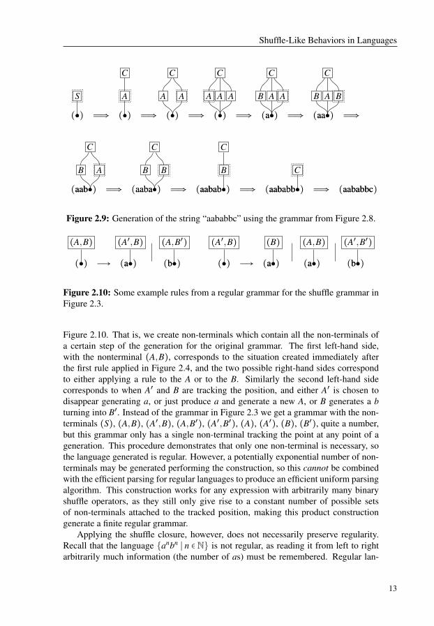
Ô⇒ (aaaabbaabbbbcc)Figure 2.9: Generation of the string “aababbc” using the grammar from Figure 2.8.
(●●)(A,B)
Ð→ (aa●●)(A′,B)
(bb●●)(A,B′)
(●●)(A′,B)
Ð→ (aa●●)(B)
(aa●●)(A,B)
(bb●●)(A′,B′)
Figure 2.10: Some example rules from a regular grammar for the shuffle grammar inFigure 2.3.
Figure 2.10. That is, we create non-terminals which contain all the non-terminals ofa certain step of the generation for the original grammar. The first left-hand side,with the nonterminal (A,B), corresponds to the situation created immediately afterthe first rule applied in Figure 2.4, and the two possible right-hand sides correspondto either applying a rule to the A or to the B. Similarly the second left-hand sidecorresponds to when A′ and B are tracking the position, and either A′ is chosen todisappear generating a, or just produce a and generate a new A, or B generates a bturning into B′. Instead of the grammar in Figure 2.3 we get a grammar with the non-terminals (S), (A,B), (A′,B), (A,B′), (A′,B′), (A), (A′), (B), (B′), quite a number,but this grammar only has a single non-terminal tracking the point at any point of ageneration. This procedure demonstrates that only one non-terminal is necessary, sothe language generated is regular. However, a potentially exponential number of non-terminals may be generated performing the construction, so this cannot be combinedwith the efficient parsing for regular languages to produce an efficient uniform parsingalgorithm. This construction works for any expression with arbitrarily many binaryshuffle operators, as they still only give rise to a constant number of possible setsof non-terminals attached to the tracked position, making this product constructiongenerate a finite regular grammar.
Applying the shuffle closure, however, does not necessarily preserve regularity.Recall that the language {anbn ∣ n ∈ N} is not regular, as reading it from left to rightarbitrarily much information (the number of as) must be remembered. Regular lan-
13

Chapter 2
guages are also closed under intersection, so if R1 and R2 are regular then so is R1∩R2.Consider the language L(a∗b∗), which contains all strings consisting of some numberof as followed by some number of bs. This is clearly regular. However,
L((ab)⊙)∩L(a∗b∗) = {anbn ∣ n ∈N}since the language L((ab)⊙) only matches strings with equally many as and bs. Assuch, since {anbn ∣ n ∈N} is not regular it follows that (ab)⊙ cannot be regular either.Notice that in terms of the sketched grammars above this corresponds to the casewhere arbitrarily many non-terminals may be attached to the tracked position, whichwould create an infinite grammar if the product construction above was attempted.
2.5 Shuffle Expressions and Concurrent Finite State Automata
The formalism that these sketched grammars are trying to imitate is Concurrent Fi-nite State Automata, one of the main subjects of Paper I. These can represent all thelanguages that can be represented by shuffle expressions, in the way the previous sec-tions sketched. They can, however, represent even more languages using one specialtrick: as was shown in the grammar in Figure 2.8 they are able to build “stacks” ofnon-terminals, where only the bottom one can be used to apply rules. By buildingthese stacks arbitrarily high, by having rules that add more and more non-terminal ontop, they are able to represent arbitrarily amounts of state (i.e. arbitrarily much infor-mation). In this way they are able to represent context-free languages, as well as theshuffle of context-free languages.
However, when this particular trick is removed we reach one of the importantmilestones. Understanding that the formalism is vaguely sketched so far (next chapterformalizes things further), let us nevertheless call it CFSA and make the followingstatement.
Theorem 2.11 (Fragment of Theorem 2 in Paper I) A language L is accepted bysome shuffle expression if and only if it is accepted by some CFSA for which thereexists a constant k such that no derivation in the CFSA has a stack of non-terminalshigher than k. ◇As such, CFSA capture both the well-known class of shuffle languages (the languagesrecognized by shuffle expressions), and permit additional language classes based on(possibly fragments of) context-free languages. This opens up questions about mem-bership problems.
2.6 Overview of Relevant Literature
These types of languages featuring shuffle, and many questions relating to them, havebeen studied in depth and over quite some time. Arguably they started with a definitionby S. Ginsburg and E. Spanier in 1965 [GS65]. The shuffle expressions, and the shufflelanguages they generate have been the primary focus of this section so far. This is the
14

Shuffle-Like Behaviors in Languages
name given to regular expressions extended with the binary shuffle operator and unaryshuffle closure, a formalism introduced by Gischer [Gis81]. These were in turn basedon an 1978 article by Shaw [Sha78] on flow expressions, which were used to modelconcurrency. The proof that the membership problem for shuffle expressions is NP-complete in general is due to [Bar85, MS94], whereas the proof that the non-uniformcase is decidable in polynomial time is due to [JS01].
Shuffle expressions are nowhere near the end of interesting aspects of the shufflehowever, even if we restrict ourselves to the focus on membership problems. A verynotable example is Warmuth and Hausslers 1984 paper [WH84]. This paper for ex-ample demonstrates that the uniform membership problem for the iterated shuffle of asingle string is NP-complete. That is, given two strings, w and v, decide whether or notw ∈ v⊙v⊙⋯⊙v. A precursor to one of the results in Paper I is due to Ogden, Riddleand Rounds, who in a 1978 paper [ORR78] showed that the non-uniform membershipproblem for the shuffle of two deterministic context-free languages is NP-complete(extended to linear deterministic context-free languages in Paper I).
Some additional examples of interesting literature on shuffle includes a deep studyon what is known as shuffle on trajectories [MRS98], where the way the shuffle mayhappen is in itself controlled by a language, and axiomatization of shuffle [EB98]. Fora longer list of references, see the introduction of Paper I.
2.7 CFSA and Context-Free Languages
As noted in Section 2.5 part of the purpose of concurrent finite-state automata isthat they permit the modeling of context-free languages, for example the language{anbn ∣ n ∈ N} (i.e. the language where some number of as are followed by the samenumber of bs), something that is not captured by shuffle expressions. A grammar forthis language is shown in Figure 2.12. A derivation in this grammar will simply gen-
(●●)S
Ð→ (aa●●)S
A
(εε) (●●)A
Ð→ (bb)Figure 2.12: A grammar in the CFSA style for the language {anbn ∣ n ∈N}.
erate some number of as while stacking up equally many A non-terminals, then whenthe S is finally replaced by ε the A non-terminals drop down and each successivelygenerates a b. In this way the (non-shuffle) language is generated. Effectively theCFSA simulates a push-down automaton.
We can easily shuffle two context-free languages in this way, by simply takinggrammars of the style of Figure 2.12 and generating their initial non-terminal (nowsuitably renamed) attached to the same position using a new initial non-terminal rule.This type of language, mixing context-free languages and shuffle, are of some practi-
15

Chapter 2
cal interest, so Paper I studies this type of situation in some depth.In fact, where shuffle expressions are regular expressions with the two shuffle
operators added, it is instructive to view general CFSA as context-free languages withthe addition of the binary shuffle operator. This part requires knowledge of context-free grammars, see e.g. [HMU03]. Consider the right-most rule in Figure 2.13, whichshowcases all the features of CFSA. Then consider the context-free grammar which
(●●)A1
Ð→ (αα) (●●)A2
Ð→ (ββ●●)B1 . . . Bn
(●●)A3
Ð→ (γγ●●)C1 . . . Cm
D
Figure 2.13: The three possible types of rules in our sketched variation of CFSAwhere α,β ,γ ∈ Σ∪{ε}. The right-most exhibits all features, where the two first areonly differentiated in that some parts don’t exist.
produces strings over the alphabet Σ∪{⊙,),(} by rewriting the CFSA rules in the wayshown in Table 2.14. Constructing a context-free grammar in this way, starting from a
Table 2.14: Context-free rules for the CFSA rule in Figure 2.13.
First rule A1→ αSecond rule A2→ β(B1⊙⋯⊙Bn)
Third rule A3→ γ(C1⊙⋯⊙Cm)D
CFSA A, one gets a context-free language L containing shuffle expressions which aresuch that L(A) =⋃{L(e) ∣ e ∈ L}. That is, when the result of evaluating all the shuffleexpressions in L are unioned together we arrive at the language generated by A.
This should serve to illustrate that all languages generated by CFSA can be viewedas “disordered” context-free languages. The above procedure generates a charac-terizing context-free language, which specifies which strings are to be shuffled to-gether to produce strings in the original CFSA. As such, for example the language{anbncn ∣ n ∈N} cannot be generated by a CFSA, as it is not context-free, nor can onearrive at it by relaxing the order of substrings in a context-free language.
2.8 Membership Problems
The membership problem for these shuffle formalisms should be divided into twoparts; the membership problem for shuffle expressions, which do not feature thecontext-free abilities of full CFSA, and the one for full CFSA.
16

Shuffle-Like Behaviors in Languages
2.8.1 The Membership Problems for Shuffle Expressions
The membership problem for shuffle expressions is already a fairly complex question.There is a sizable body of literature, and Paper I studies one fragment of the problem.
• The non-uniform membership problem is decidable in polynomial time [JS01].The algorithm relies on permitting each symbol read (or generated) to producesome large number of potential states, which limits the complexity in terms ofthe length of the string but explodes the complexity in terms of the size of theexpression.
• Unsurprisingly, in view of the above, the general uniform membership problemis NP-complete [Bar85, MS94].
These two pieces paint a fairly clear picture; if we wish to check membership (orparse) a string with respect to a shuffle expression it can be done reasonably efficientlyif the string is much larger than the shuffle expression. However, this does not revealthe exact way in which the complexity depends on the expression. Notably, regularexpressions are (trivially) shuffle expressions, and for regular expressions the uniformmembership problem is not very difficult. Paper I explores how the structure of theexpression affects the complexity of the problem. See Section 2.9.
2.8.2 The Membership Problems for General CFSA
The membership problem for CFSA is NP-hard even in very restrictive cases, such aswhere at most two non-terminals are ever attached to a position. It may therefore besurprising that the problem is in NP. The overall construction hinges on limiting thesize of the trees of non-terminals generated by parsing a certain string, which relieson a careful case-by-case analysis of symmetries in how non-terminals may be gener-ated. This means that even if far more (seemingly) complex CFSA are considered theproblem does not become substantially harder. All of this is treated in Paper I, whichSection 2.9 now takes a deeper look into.
2.9 Contributions In the Area of Shuffle☆This section provides, as denoted by the star, a slightly more formal treatment of thecontributions to the area of shuffle that have been made in (the papers included in) thiswork. We need some additional definitions to start with.
2.9.1 Definitions and Notation
Let N+ denote N∖{0}. A tree with labels from an alphabet Σ is a function t ∶N → Σ,where N ⊆N∗+ is a set of nodes which are such that
• N is prefix-closed, i.e., for every v ∈N and i ∈N+, vi ∈N implies that v ∈N, and
• N is closed under less-than, i.e., for all v ∈ N∗+ and i ∈ N+, v(i+1) ∈ N impliesvi ∈N.
17

Chapter 2
Let N(t) denote the set of nodes in the tree t. The root of the tree is the node ε , and viis the ith child of the node v. t/v denotes the tree with N(t/v) = {w ∈N∗+ ∣ vw ∈ N(t)}and (t/v)(w) = t(vw) for all w ∈ N(t/v). The empty tree, denoted tε , is a specialcase, since N(tε) = ∅ it cannot be a subtree of another tree. Given trees t1, . . . ,tn anda symbol α , we let α[t1, . . . ,tn] denote the tree t with t(ε) = α and t/i = ti for alli ∈ {1, . . . ,n}. The tree α[] may be abbreviated by α . Given an alphabet Σ, the setof all trees of the form t ∶N → Σ is denoted by TΣ. For trees t,t′ and v ∈ N(t) let tv↦t′be the tree resulting from replacing the node at v by t′ in t. That is, tε↦t′ = t′, andtiv↦t′ = t(ε)[t/1, . . . ,(t/i−1),(t/i)v↦t′ ,(t/i+1), . . . ,t/n] for iv ∈ N(t) and i ∈N+. Fortv↦tε the subtree at v is deleted (e.g. α[t1,t2,t3]2↦tε = α[t1,t3]).2.9.2 Concurrent Finite State Automata
With this we can make a formal definition of the concurrent finite state automataalready sketched. These automata are the subject at the heart of Paper I.
Definition 2.15 A concurrent finite state automaton is a tuple A = (Q,Σ,S,δ) whereQ is a finite set of states, Σ is the input alphabet, S ∈ Q is the initial state, and δ ∶Q×(Σ∪{ε})×TQ are the rules.
A derivation in A is a sequence t1, . . . ,tn ∈ TQ such that t1 = S[] and tn = tε . For eachi < n the step from t = ti to t′ = ti+1 is such that there is some (q,α,t′′) ∈ δ and v ∈N(ti)such that t/v = q[] and t′ = tv↦t′′ . Applying this rule reads the symbol α (nothing ifα = ε). L(A) is the set of all strings that can be read this way.
We only permit four types of rules in δ . Deleting rules of the form (q,ε,tε) ∈ δ .Horizontal rules of the form (q,α,q′[]) ∈ δ . Vertical rules of the forms (q,α,q′[p1]) ∈δ and (q,α,q′[p1, p2]) ∈ δ . Finally the closure rules, where (q,α,q′[p1, . . . , p1]) ∈ δfor every number of repetitions of p1s, greater or equal to zero. ◇We treat the in practice infinite set of rules for the closure rules as a schema (i.e.they count as a constant number of rules for the purposes of defining the size of theautomaton).
Using this definition it should be easy to see how the rules in Figure 2.13 can beconstructed. The graphical rules cheat by ignoring the possibility that α = ε , while per-mitting e.g. generating siblings without a root (effectively having rules (q,α, p1 p2)),but it is trivial to add an additional state that serves as root for the subtree with only adeleting rule defined.
Notice that the rules overlap a bit, in that the closure schema is unnecessary if weare allowed to replace (q,α,q′[p1, . . . , p1]) with (q,α,q′[q′′, p1]) where q′′ is a newstate with only two rules, (q′′,ε,tε) and (q′′,ε,q′′[q′′, p1]). However, the context-freelanguages are precisely those that can be recognized by a CFSA where every (q,α,t) ∈δ has no node with more than one child in t, and we often wish to syntactically restrictCFSA to not permit context-free languages, recreating the shuffle languages. We dothis as follows: a configuration is acyclic if for every v ∈ N(t) it holds that t(v) doesnot occur in t/vi for any i, the shuffle languages are then precisely the CFSA where allconfigurations are acyclic. The closure-free shuffle languages are those recognizableby a CFSA with a finite (schema-free) δ and all reachable configurations acyclic.
18

Shuffle-Like Behaviors in Languages
2.9.3 Properties of CFSA
Paper I proves a number of relevant properties about CFSA. Notably they are closedunder union, concatenation, Kleene closure, shuffle, and shuffle closure (i.e., if A andA′ are CFSA then there exists a CFSA A′′ such that e.g. L(A′′) = L(A)⊙L(A′)),but not under complementation or intersection (so there exists some A and A′ suchthat there exists no CFSA recognizing the language e.g. L(A)∩L(A′)). Emptiness ofCFSA is decidable in polynomial time, and the CFSA generate only context-sensitivelanguages.
2.9.4 Membership Testing CFSA
Membership in general CFSA. With this done we can consider uniform mem-bership testing for general CFSA, one of the core results of Paper I. Since even aseverely restricted case of CFSA already have a NP-complete uniform membershipproblem [Bar85, MS94], which serves as a lower bound, it is a pleasant surprise thatthe general problem is in NP, as the restricted cases appear so relatively restrictive. Anon-deterministic polynomial time algorithm can simply guess which rules to applyto accept a string, as long as the number of rules necessary (i.e. the sequence t1, . . . ,tnin Definition 2.15) is polynomial in the length of the string. The only way this mightnot happen is if a lot of ε-rules are required. A simple polynomial rewriting procedureon A solves this, based on statements such as “if rules from δ can rewrite q[] into q′[]without reading a symbol, include (q,ε,q′[]) in δ .” This ensures that if a derivationof a string exists in A then a short one exists.
Membership in the shuffle of shuffle languages and context-free languages. TheCFSA model goes on to be used to prove a number of other membership problemresults. One interesting case is the shuffle of a shuffle language and a context-freelanguage, i.e., membership for the CFSA where every configuration tree (except thefirst one and the last one where things are getting set up and dismantled) is of theform q[t1,t2] where t1 is acyclic and N(t2) ⊂ 1∗ (that is, no node in t2 has more thanone child). This proof is rather more involved, and relies on finding a number ofsymmetries in the way the tree corresponding to the shuffle language (i.e. t1 here) canbehave. Notably it relies on defining an equivalence relation on nodes in the tree, i.e.,if we have t(v) = t(v′) what we do to v and v′ is interchangeable. Most notably, if wein two places apply a rule schema (q,α,q′[p1, . . . , p1]) there is no point in generatingp1 instances in both places, we might as well pick one of the places and generate allthe instances of p1 necessary. In fact, in the procedure we can just remember “aslong as this node is still here we can assume we have any necessary number of p1instances”. In this way the number of possibilities are limited in such a way that aCocke-Younger-Kasami-style table can be established for parsing. While polynomialthe degree of the polynomial is very substantial, an efficient algorithm is left as futurework.
The hardness of context-free shuffles. Another of the core results of Paper I is aproof that there exist two deterministic linear context-free (DLCF) languages L and L′
19

Chapter 2
such that the membership problem for L⊙L′ is NP-complete. That is, the non-uniformmembership problem for the shuffle of two DLCF languages is NP-complete. Theproof relies on the following. We can construct a DLCF language L which consists ofstrings of the following form:
[0][1]⋯[1][1]´¹¹¹¹¹¹¹¹¹¹¹¹¹¹¹¹¹¹¹¹¹¹¹¹¹¹¹¹¹¹¹¹¹¹¹¸¹¹¹¹¹¹¹¹¹¹¹¹¹¹¹¹¹¹¹¹¹¹¹¹¹¹¹¹¹¹¹¹¹¹¶C1
$[0][1]⋯[1][1]´¹¹¹¹¹¹¹¹¹¹¹¹¹¹¹¹¹¹¹¹¹¹¹¹¹¹¹¹¹¹¹¹¹¹¹¸¹¹¹¹¹¹¹¹¹¹¹¹¹¹¹¹¹¹¹¹¹¹¹¹¹¹¹¹¹¹¹¹¹¹¶C2
$⋯$[0][1]⋯[1][0]´¹¹¹¹¹¹¹¹¹¹¹¹¹¹¹¹¹¹¹¹¹¹¹¹¹¹¹¹¹¹¹¹¹¹¹¸¹¹¹¹¹¹¹¹¹¹¹¹¹¹¹¹¹¹¹¹¹¹¹¹¹¹¹¹¹¹¹¹¹¹¶C′2
$[0][1]⋯[1][1]´¹¹¹¹¹¹¹¹¹¹¹¹¹¹¹¹¹¹¹¹¹¹¹¹¹¹¹¹¹¹¹¹¹¹¹¸¹¹¹¹¹¹¹¹¹¹¹¹¹¹¹¹¹¹¹¹¹¹¹¹¹¹¹¹¹¹¹¹¹¹¶C′1
where each bit-string is a polynomial-length Turing machine configuration, and C′1 is
the (reversed) configuration the Turing machine reaches taking one step from C1, andsimilarly C′
2 is one step from C2 (and so on nested inwards). The rules of the Turingmachine are encoded in L. The language class is not powerful enough to relate C1 andC2, all it can do by itself is take a single step. We can however also construct a DLCFlanguage L′ which recognizes all strings
$[0][1]⋯[0][1]´¹¹¹¹¹¹¹¹¹¹¹¹¹¹¹¹¹¹¹¹¹¹¹¹¹¹¹¹¹¹¹¹¹¹¹¸¹¹¹¹¹¹¹¹¹¹¹¹¹¹¹¹¹¹¹¹¹¹¹¹¹¹¹¹¹¹¹¹¹¹¶P1
$[1][1]⋯[1][1]´¹¹¹¹¹¹¹¹¹¹¹¹¹¹¹¹¹¹¹¹¹¹¹¹¹¹¹¹¹¹¹¹¹¹¹¸¹¹¹¹¹¹¹¹¹¹¹¹¹¹¹¹¹¹¹¹¹¹¹¹¹¹¹¹¹¹¹¹¹¹¶P2
$⋯$[1][1]⋯[1][1]´¹¹¹¹¹¹¹¹¹¹¹¹¹¹¹¹¹¹¹¹¹¹¹¹¹¹¹¹¹¹¹¹¹¹¹¸¹¹¹¹¹¹¹¹¹¹¹¹¹¹¹¹¹¹¹¹¹¹¹¹¹¹¹¹¹¹¹¹¹¹¶P′2
$[1][0]⋯[1][0]´¹¹¹¹¹¹¹¹¹¹¹¹¹¹¹¹¹¹¹¹¹¹¹¹¹¹¹¹¹¹¹¹¹¹¹¸¹¹¹¹¹¹¹¹¹¹¹¹¹¹¹¹¹¹¹¹¹¹¹¹¹¹¹¹¹¹¹¹¹¹¶P′1
which are such that P′1 is P1 reversed, and P′2 is P2 reversed, and so on inwards. Atthe center there is one extra string of the form ([0]∣[1])∗, entirely arbitrary. Nowconstruct the string
[0]⋯[0]´¹¹¹¹¹¹¹¹¹¹¹¹¸¹¹¹¹¹¹¹¹¹¹¹¶I
$[[01]]⋯[[01]]$$⋯$$[[01]]⋯[[01]]where I is filled with the initial Turing machine configuration we are interested in.Then check if this string is in L⊙L′. What will happen is that L and L′ will have to“share” every [[01]]⋯[[01]] substring (since neither can by itself produce e.g. [[),each producing half the brackets and binary digits, forcing the other to produce itscomplement. The initial I must be produced by L, as L′ requires a leading $, whichmakes L produce the result of taking the first step of the Turing machine in the last[[01]]⋯[[01]] section, which leaves the complement for L′ to produce in the lastsection, which will make it produce the complement in the first [[01]]⋯[[01]] section,forcing L to produce the same configuration in that first sectiont that it produced in thelast section. This makes it produce the result of taking another computation step inthe second-to-last [[01]]⋯[[01]] section, which L′ then copies, and so on. In this waythe shuffle will cooperate to perform an arbitrary (non-deterministic) Turing machinecomputation for polynomially many steps, making the membership problem NP-hard.This is non-uniform as the Turing machine coded in L may be one of the universalmachines, which reads its program from the input I.
2.9.5 The rest of Paper I.
Paper I has a number of further results, including a fixed parameter analysis of parsingshuffle expressions with the number of shuffle operators which is discussed in brief inSection 3.5.1. In addition the paper discusses the uniform membership problem for
20
Shuffle-Like Behaviors in Languages
the shuffle of a context-free language and a regular language. That is, a context-freegrammar G, a finite automaton A and a string w are given as input, and the decisionproblem is checking whether w ∈ L(G)⊙L(A)). An important point in this context isthat L(G)⊙L(A) is a context-free language for all G and A. This can be shown bya simple product construction. This, however, raises a question discussed in anotherpaper.
2.9.6 Language Class Impact of Shuffle
Paper V also considers shuffle, but here the question is of a more abstract nature.The claim studied is, for two context-free languages L ⊆ Σ∗ and L′ ⊆ Γ∗ (with Σ∩Γ =∅) is L⊙ L′ ∉ CF unless either L ∈ Reg or L′ ∈ Reg? That is, if the shuffle of twocontext-free languages is context-free must one of the languages be regular? Theauthor conjectures that this is indeed the case, but Paper V gives only a conditionaland partial proof.
21

Chapter 2
22

CHAPTER 3
Synchronized Substrings inLanguages
In this chapter we take a look at what can be described as formalisms with synchro-nized substrings. A single sequence of derivation decisions which (may) have effectsin several places of a string. This is most easily illustrated by extending our runningsketched formalism to generate such languages.
3.1 Sketching a Synchronized Substrings Formalism
3.1.1 The Graphical Intuition
In this section the grammars introduced in Figure 1.3 will be extended in a differentway from the preceding shuffle chapter. In this new grammatical formalism there maynot be more than one non-terminal attached to a position (i.e. to a bullet), nor may wehave non-terminals depend on each other. That is, the “stacking” of non-terminals ofFigure 2.8 is no longer permitted.
The new grammatical formalism for this chapter instead generalize the regulargrammars in some new ways, which will pave the way to rules of the following form.
(●●)E
Ð→ (aaaa●●●●aaaa●●bb●●bbbb)DE
• Positions (i.e. bullets) may now occur anywhere in the string, not just at theend. There may be any number of positions on the right-hand side of rules.
• Each non-terminal may be attached to multiple positions. We say that the non-terminal tracks, or controls, those positions. This in turn means that the left-hand sides may also contain multiple positions (the number controlled by thenon-terminal being replaced).
We assume that each non-terminal always tracks the same number of positions (so if Atracks 3 positions in one rule it will always track 3 positions). See Figure 3.1 for a firstexample of a grammar of this new kind. An example derivation using this grammar isshown in Figure 3.2.
23
Chapter 3
(●●)S
Ð→ (●●●●●●)A
(●●,●●,●●)A
Ð→ (aa●●,,bb●●,,cc●●)A
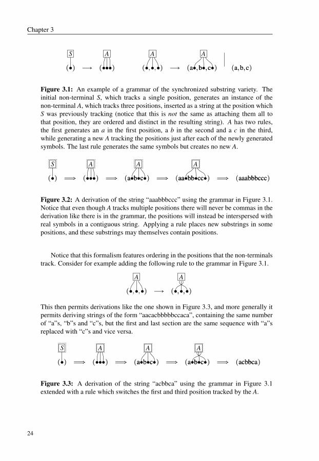
(aa,,bb,,cc)Figure 3.1: An example of a grammar of the synchronized substring variety. Theinitial non-terminal S, which tracks a single position, generates an instance of thenon-terminal A, which tracks three positions, inserted as a string at the position whichS was previously tracking (notice that this is not the same as attaching them all tothat position, they are ordered and distinct in the resulting string). A has two rules,the first generates an a in the first position, a b in the second and a c in the third,while generating a new A tracking the positions just after each of the newly generatedsymbols. The last rule generates the same symbols but creates no new A.
(●●)S
Ô⇒ (●●●●●●)A
Ô⇒ (aa●●bb●●cc●●)A
Ô⇒ (aaaa●●bbbb●●cccc●●)A
Ô⇒ (aaaaaabbbbbbcccccc)Figure 3.2: A derivation of the string “aaabbbccc” using the grammar in Figure 3.1.Notice that even though A tracks multiple positions there will never be commas in thederivation like there is in the grammar, the positions will instead be interspersed withreal symbols in a contiguous string. Applying a rule places new substrings in somepositions, and these substrings may themselves contain positions.
Notice that this formalism features ordering in the positions that the non-terminalstrack. Consider for example adding the following rule to the grammar in Figure 3.1.
(●●,●●,●●)A
Ð→ (●●,,●●,,●●)A
This then permits derivations like the one shown in Figure 3.3, and more generally itpermits deriving strings of the form “aacacbbbbbccaca”, containing the same numberof “a”s, “b”s and “c”s, but the first and last section are the same sequence with “a”sreplaced with “c”s and vice versa.
(●●)S
Ô⇒ (●●●●●●)A
Ô⇒ (aa●●bb●●cc●●)A
Ô⇒ (aa●●bb●●cc●●)A
Ô⇒ (aaccbbbbccaa)Figure 3.3: A derivation of the string “acbbca” using the grammar in Figure 3.1extended with a rule which switches the first and third position tracked by the A.
24

Synchronized Substrings in Languages
3.1.2 Revisiting the Mapped Copies of Example 1.1
Example 1.1 illustrates a trivial case of synchronized substrings formalisms, where asequence of symbols is chosen, and two different symbol mappings create two dif-ferent strings, which are concatenated to produce an output string. Let us recall ithere.
Example 3.4 (Mappings of copy-languages) Given two mappings σ1,σ2 from {a,b}to arbitrary strings and a string w decide whether there exists some α1, . . . ,αn ∈ {a,b}such that σ1(α1)⋯σ1(αn) ⋅σ2(α1)⋯σ2(αn) =w. ◇Let us look at how
1. we can model this type of language by a grammar, and,
2. parsing may be performed, in both the uniform and non-uniform case.
3.1.3 Grammars for the Mapped Copy Languages
Here we have two alphabets, the “internal” alphabet Γ = {a,b} as well as the usual Σ.In addition we have two mappings from Γ to strings in Σ. Let wa = σ1(a), wb = σ1(b),va = σ2(a) and vb = σ2(b). Then the grammar in Figure 3.5 generates the language ofthe strings that the procedure in Example 1.1 yields.
(●●)S
Ð→ (●●●●)A
(●●,●●)A
Ð→ (wawa●●,,vava●●)A
(wbwb●●,,vbvb●●)A
(εε,,εε)Figure 3.5: A synchronized substring-type grammar for the language that the proce-dure sketched in Example 1.1 can produce. Notice that wa, va, wb and vb are stringsderived from the mappings σ1 and σ2, rather than symbols in their own right.
3.1.4 Parsing for the Mapped Copy Languages
Let us consider the uniform parsing problem for this class of grammars (i.e., thosethat can be generated by some choice of σ1 and σ2 in the above construction). We candivide the parsing problem into two parts:
1. We need to find the position at which the concatenation happens. That is, let Gbe the grammar constructed as in Figure 3.5 for some σ1 and σ2, then, to decideif some w belongs to L(G) we need to tell if there is some way to divide w intotwo, w = xy, such that σ1(v) = x and σ2(v) = y for some v ∈ {a,b}∗.
2. The second part is finding the actual v ∈ {a,b}∗.
Solving the second part effectively solves the first, in the sense that if we are given vwe will be able to tell where the concatenation happens by simply computing σ1(v)and σ2(v).
25

Chapter 3
However, it might be easier to find v if the point of concatenation is found. Weare in fact primarily concerned about whether parsing can be done in polynomial timeor not, and if we can compute v in polynomial time given the point of concatenationwe can solve the whole problem in polynomial time, as there are only linearly manypositions at which the concatenation may occur. That is, we can simply for eachpossible way of dividing w into xy try to compute a v for this x and y. This exhaustivesearch at most makes the membership problem linearly more expensive.
The full algorithm for this toy example is in fact fairly simple. It will, however,serve to illustrate the more general algorithms later, where the directed graph con-struction will be replaced by something similar but more advanced.
Algorithm 3.6 (Parsing for Example 1.1)1: function PARSECOPYMAP(string w ∈ Σ∗, σ1 ∶ {a,b}→ Σ∗, σ2 ∶ {a,b}→ Σ∗)2: let α1⋯αn =w (i.e., each αi is a symbol in Σ).3: let G be a digraph with nodes {(p,q) ∣ p,q ∈ {0, . . . ,n}} and no edges.4: for p,q, p′,q′ ∈ {0, . . . ,n} do5: if (σ1(a) = αp+1⋯αp′ and σ2(a) = αq+1⋯αq′ ) or6: (σ1(b) = αp+1⋯αp′ and σ2(b) = αq+1⋯αq′ ) then7: add an edge from (p,q) to (p′,q′) to G8: end if9: end for
10: for i ∈ {0, . . . ,n} do11: if REACHABLE(G, (0, i), (i,n)) = True then12: return True13: end if14: end for15: return False16: end function
REACHABLE is a function which takes a graph G and two nodes v and w and checksif w can be reached from v following the edges. Notice that we abuse the subscripts inthe algorithm, so αp+1⋯αp′ for p ≥ p′ will be an empty string.
To quickly outline the algorithm, in lines 4–9 the graph G is constructed in such away that a node (p′,q′) is only reachable from (p,q) if the substrings αp+1⋯αp′ canbe generated by σ1(v) and αq+1⋯αq′ can be generated by σ2(v) for some common v.Once this graph is constructed lines 10–14 simply test all ways to cut the initial stringinto two pieces and checks on the graph if the resulting two strings can correspond toa common original string mapped through σ1 and σ2.
Notice that the graph will be polynomial in the size of the string to be parsed,and computing reachability on a directed graph is very cheap. Also notice that thisalgorithm as written is just a membership test, but making it parsing amounts to simplyoutputting the path in G found when line 11 succeeds.
26

Synchronized Substrings in Languages
3.2 The Broader World of Mildly Context-Sensitive Languages
The above may seem like trivialities, but it appears to be at the core of the difficultyin deciding membership for the general class of formalisms along these lines. Theformalism sketched here (exemplified by the grammar in Figure 3.5) is intended toimitate a hyperedge replacement grammar (see e.g. [DHK97]) generating a string, butthat formalism is equivalent to a large class of other formalisms.
3.2.1 The Mildly Context-Sensitive Category
All the formalisms discussed in this chapter fall within the category “mildly context-sensitive”, defined by Aravind Joshi in [Jos85]. A language class L is defined by Joshito be mildly context-sensitive if and only if all the following hold.
1. At least one language in L features limited cross-serial dependencies.
2. All languages L in L have a semi-linear set {∣w∣ ∣ w ∈ L}. That is, the lengthsof strings in the language form a union of a finite number of linear sequences,{s1+ ik1 ∣ i ∈N}∪⋯∪{sn+ ikn ∣ i ∈N}.
In addition the following two requirements are implicit but clearly required in [Jos85]
3. All L ∈ CF are in L , that is, a mildly context-sensitive formalism must be ableto represent all context-free languages (recall Section 2.7).
4. The non-uniform membership problem for languages in L is decidable in poly-nomial time.
Requirement 1 needs some further explanation. It refers to a certain type of substringsynchronization that Joshi derives from the tree-adjoining grammar formalism thathe uses in that paper. The description is fairly involved, but one key detail is thatlanguages of the form anbncn may be in such a class, but anbnanbnanbn⋯ may not.This statement may be transferred to the formalism we have sketched by noting thatfor every such grammar there exists some constant k such that no non-terminal tracksmore than k positions, which makes it impossible to generate e.g.
anbn⋯anbn´¹¹¹¹¹¹¹¹¹¹¹¹¹¹¹¹¹¹¹¹¹¹¸¹¹¹¹¹¹¹¹¹¹¹¹¹¹¹¹¹¹¹¹¹¶k+1 copies
.
3.2.2 The Mildly Context-Sensitive Classes
There are at least two different classes of languages with published formalisms that fitclearly into the mildly context-sensitive definition.
1. The first is the motivating class, into which tree-adjoining grammars [JLT75]which Joshi used when first defining the category, fall. All the following for-malisms are equivalent [JSW90] (that is, they define the same language class):linear indexed grammars [Gaz88], combinatorial categorial grammars [Ste87]and head grammars [Pol84].
27

Chapter 3
2. The second class still fulfills all the requirements outlined by Joshi, but is strictlymore powerful (i.e. every language that can be generated by e.g. a head grammarcan be generated by any of these formalisms). These formalisms include linearcontext-free rewriting systems [Wei92]1, deterministic tree-walking transduc-ers [Wei92], multicomponent tree-adjoining grammars [Jos85, Wei88], multiplecontext-free grammars [SMFK91, Got08], simple range concatenation gram-mars [Bou98, Bou04, BN01, VdlC02] and string-generating hyperedge replace-ment grammars [Hab92, DHK97].
It is interesting to note that while the mildly context-sensitive definition requires a non-uniform membership problem (i.e. the membership problem where the string, but notthe grammar/automaton, is included in the input, recall Definitions 1.7 and 1.8) that issolvable in polynomial time, all the listed formalisms above have an NP-hard uniformmembership problem. The way that the grammars perform concatenation, notablyhow many positions each non-terminal keeps track of (or, in Joshis terminology, theextent of the cross-serial dependencies), play a big part in how difficult the uniformmembership problem becomes.
Going through all of these formalisms is not time well spent for an introductorytext like this, but in the next section we will make the connection between the sketchedformalism of Figure 3.1 and string-generating hyperedge replacement grammars.
3.3 String-Generating Hyperedge Replacement Grammars
The formalism sketched in Figures 3.1–3.5 is more or less a direct copy of hyperedgereplacement grammars tuned for string generation. This formalism constructs a di-rected graph by having hyperedges (that is, edges that connect an arbitrary numberof nodes) labeled with non-terminal symbols, and having rules that replace these bynew subgraphs connected to the nodes the hyperedge was connected to. So, the ruleapplication (using a rule from Figure 3.1)
(aa●●bb●●cc●●)A
Ô⇒ (aaaa●●bbbb●●cccc●●)A
actually corresponds to rewriting the directed graph
a b c
A
where the box labeled by A now represents a hyperedge which is connected to 6 nodes,into this graph
1 References are for the most part not to the original definitions, but rather to sources where they aredescribed and related to the broader class at hand.
28

Synchronized Substrings in Languages
a a b b c c
A
by the hyperedge labeled A being replaced by attaching new nodes and edges to thepositions the original hyperedge was attached to, and attaching a new hyperedge (alsolabeled A). To make this perfectly formal we also need to number the nodes, or oth-erwise somehow distinguish between them, which we manage to avoid graphically inthe string case by just keeping track of things left-to-right.
Notice that while the non-uniform membership problem is polynomial for string-generating hyperedge replacement grammars it very quickly becomes NP-hard whenthe grammar are allowed to generate graphs even a little bit more complex than thesestring-representing directed chains. In fact, if the grammar is allowed to make multiplechains, that is, creating a graph consisting of the union of directed chains, by simplyhaving the hyperedge replacement rules leaving pieces unconnected, the non-uniformmembership problem becomes NP-complete [LW87].
In addition note that for a hyperedge replacement grammar to generate a stringit will necessarily have to keep track of both sides of each “gap” corresponding to aposition, as is sketched in the above figures. If it loses track of a node that is supposedto be internal to the string it becomes impossible to later join it up to the other partsgenerated, and the graph becomes a set of multiple chains.
We will next take a look at a general non-uniform parsing algorithm for string-generating hyperedge replacement grammars (the informal flavor used here). Thisconstruction is from 2001 by Bertsch and Nederhof [BN01] (this is not the earliest ormost efficient parsing algorithm of this type, but a straightforward and clear one).
3.4 Deciding the Membership Problem
3.4.1 Deciding Non-Uniform Membership
Origins of the Algorithm The construction from [BN01] is here modified a bit forclarity and to fit into the approach we use. In its original form the algorithm takesthe grammar G (for which membership should be decided) and a string w, and fromthese two constructs a new grammar G′, which is empty if and only if w ∉ L(G). Inthis way it reduces the problem of deciding membership for one grammar to the prob-lem of deciding emptiness for another. More specifically the grammar G is one ofthe mildly context-sensitive formalisms (the algorithm is originally defined in termsof Range Concatenation Grammars, but here we opt to continue with the equiva-lent string-generating hyperedge replacement grammars) and the constructed gram-mar G′ is a context-free grammar, for which emptiness testing (i.e. computing whetherL(G′) = ∅) is very easy. However, as context-free grammars are a subset of the hy-peredge replacement grammars (and emptiness testing is just as easy for hyperedgereplacement grammars) we will not differentiate between the formalisms.
29

Chapter 3
Deciding Emptiness Emptiness-checking a hyperedge replacement grammar is veryeasy. Start by letting all non-terminals be unmarked. For each rule, if the left-hand isunmarked but the right-hand side contains no unmarked non-terminals mark the non-terminal on the left-hand side and start over the looping through the rules from the firstone. If we make it through all the rules without marking a non-terminal we are done,and the language generated by the grammar is empty if and only if S is still unmarked.This algorithm is clearly in O(n2) where n is the number of rules, as it is a loop thatis restarted at most n times (sooner or later all the non-terminals have been marked).
Reducing Membership to Emptiness It is time to solve the membership problemfor string-generating hyperedge replacement grammars. Let G be the grammar, andα1⋯αn (αi ∈ Σ for each i) the string for which we wish to check whether α1⋯αn ∈L(G). To decide this we will construct a new grammar G′ such that L(G′) ≠∅ if andonly if α1⋯αn ∈ L(G) (specifically, L(G′) = {ε} otherwise). The construction of G′should be reminiscent of the construction of the graph in Algorithm 3.6.
G′ will be constructed in such a way that if G contains a non-terminal A which con-trols k positions (i.e. there are k positions on the left hand side of rules for A) then G′contains one non-terminal A(p1,q1),...,(pk,qk) for each p1,q1, . . . . . . , pk,qk ∈ {0, . . . ,n},such that p1 ≤ q1, . . . , pk ≤ qk. The logic will be, if the non-terminal A(p1,q1),...,(pk,qk)can generate any strings, then the non-terminal A in the original grammar G is able togenerate the strings αp1⋯αq1 , . . . ,αpk⋯αqk . The most direct rule to include in G′ thenbecomes that if
(●●,, . . .. . .,,●●)A
Ð→ (αp1+1⋯αq1αp1+1⋯αq1 ,, . . .. . .,,αpk+1⋯αqkαpk+1⋯αqk). . .
is a rule in G then
(●●)A(p1,q1),...,(pk,qk)
Ð→ (εε)is a rule in G′. That is; if A can generate the substrings αp1+1⋯αq1 through αpk+1⋯αqk ,then A(p1,q1),...,(pk,qk) can generate the empty string (we could select any string as onlyemptiness is of interest). Similarly, for example, if there is a rule in G of the form
(●●,●●)A
Ð→ (●●●●,,●●●●●●)B C D
then, for all p1,q1, p2,q2 ∈ {0,n}, and k1,k2,k3 ∈ {0,n}, such that p1 ≤ k1 ≤ q1, andp2 ≤ k2,k3 ≤ q2 there is a rule
(●●)A(p1,q1),(p2,q2)
Ð→ (●●●●●●)B(p1,k1),(k3,q2) C(k1,q1),(p2,k2) D(k2,k3)
.
30

Synchronized Substrings in Languages
That is, the p1,q1, p2,q2 decide the substrings checked by the left-hand side, and k1is the position between p1 and q1 where the substring goes from being generated bythe B and the C, and similarly for k2 and k3 with the two concatenation points in thesecond substring. This generalizes to arbitrary rules in the obvious way, when non-terminals and symbols are mixed one additionally needs to check that the symbolsgenerated correspond correctly to the symbols in α1⋯αn.
As such, if each of the B, C and D non-terminals can generate their respectivesubstrings then the right-hand side can generate the empty string, meaning that the Acan generate the whole. Finally, add the rule
(●●)S
Ð→ (●●)S(0,n)
to G′, that is, the initial non-terminal goes to the non-terminal that checks if the non-terminal S in G can generate the substring α0+1⋯αn, i.e., the whole string.
Following this procedure G′ will be able to generate the empty string if and only ifG can generate the string α1⋯αn. It should be clear that the size of G′ is on the orderof O(nc) where c is polynomial in the size of the grammar G. Notably c increaseswith the number of positions tracked by non-terminals in G.
However, we were considering the non-uniform membership problem, and as suchwe view G as a constant, which in turn means that c is viewed as a constant. Itfollows that O(nc) is a polynomial, and, as established above, deciding emptiness ispolynomial, making for a membership algorithm that is polynomial.
3.4.2 Deciding Uniform Membership
Deciding the uniform membership problem for our sketched grammatical formalismappears to be extremely hard, a proof that LCFRS parsing is PSPACE-hard is givenin [KNSK92]. This makes it extremely unlikely that an efficient algorithm exists. Thebest known algorithms (see e.g. [SMFK91] and Paper II for more references) for theproblem are in O(mn f(r+1)) where m is the size of the grammar, n the size of theinput string, and f and r are two very specific properties of the grammar, the fan-outand the rank of the grammar respectively. Before we get further into the explanationit is important to note that since f and r are values depending on the grammar thealgorithm is in O(nm) as well, that is, the length of the string raised to the size of thegrammar. However, it turns out that in practice the fan-out and rank tend to be smallcompared to the size of the full grammar, so it is a useful distinction to separate themout.
In short, the rank of a grammar is the maximum number of non-terminals occur-ring on the right hand side of a rule. The fan-out is the maximum number of positionsa non-terminal tracks. So for example a grammar G containing the rule
(●●,●●,●●,●●)A
Ð→ (aa●●●●●●,,●●,,aabbcc,,cc●●cc)BC D
31

Chapter 3
implies that it has rank at least 3, since the right-hand side has three non-terminals,and fan-out at least 4, since A controls four positions. These are “at least” since otherrules may contain more non-terminals or more positions tracked.
3.4.3 On the Edge Between Non-Uniform and Uniform
So far we have seen that the problem is polynomial when the grammar is left out of theinput entirely, and an algorithm that is unquestionably exponential when the grammaris included. However, this distinction, where some aspects of the grammar is separatedout to illustrate that it is not exponential in the “worst” way, is a bit blunt and imprecisea way of viewing the complexity. For example, if the total number of rules were inthe exponent many practical grammars would have very problematic running times,whereas if the number of symbols in the alphabet is the part in the exponent thingsmay not be nearly as problematic.
For a deeper look in this direction, we now give a slightly deeper summary of theresults in Paper II, with explanations of some of the supporting theory.
3.5 Contributions in Fixed Parameter Analysis of Mildly Context-Sensitive Languages☆
We take this opportunity to briefly explain fixed parameter complexity, as it is neces-sary to appreciate the contents of Paper II, and may not be common knowledge. Seee.g. [FG06] for a full introduction.
3.5.1 Preliminaries in Fixed Parameter Tractability
In classical complexity theory a problem may be viewed as a set of all positive in-stances P ⊆ I, where I is the set of all possible instances. For example, we may have Ibe all graphs and P be the set of all graphs which have a Hamiltonian path. A decisionprocedure for the problem is then a program that computes a function a ∶ I→ {yes,no}such that P = {p ∈ I ∣ a(p) = yes}. The running time of the program is then analyzedas a function in ∣p∣. For two problems P ⊆ I and P′ ⊆ I′ a polynomial time reductionis a function r ∶ I → I′, computable in polynomial time such that p ∈ P⇔ r(p) ∈ P′. Apolynomial time reduction r from P to P′ implies that the fastest decision procedurefor P cannot be more than polynomially slower than the fastest for P′.
A parameterized problem is viewed as a set P ⊆ I ×N, where I is again the setof all problem instances and the integer is what is called the parameter. A decisionprocedure for R again computes a function a ∶ I ×N → {yes,no}, but now the timeof deciding a(p,k) is described in both ∣p∣ and k. If a runs in time f (k) ⋅ ∣p∣O(1)for any computable function f ∶ N → N the problem is said to be fixed-parametertractable (FPT); that is, intuitively, for a small parameter the problem is basicallypolynomial. The way the parameter is chosen has a large impact on how the analy-sis behaves. Notably, taking any problem P ⊆ I and constructing the parameterizedproblem {(p, ∣p∣) ∣ p ∈ P} ⊆ I ×N yields a fixed-parameter tractable problem for ev-ery decidable P. A FPT reduction from P ⊆ I ×N to P′ ⊆ I′ ×N is a program which
32

Synchronized Substrings in Languages
computes a function r ∶ (I ×N)→ (I′ ×N) such that, (i) r(p,k) is computable in timef (k) ⋅ ∣p∣O(1) for some computable function f ; (ii) (p,k) ∈ P⇔ r(p,k) ∈ P′; and; (iii)there exists a computable function g such that for all (p′,k′) = r(p,k) it holds thatk′ ≤ g(k).
The parameter is normally chosen as some minor aspect of the problem. A classiccase is the vertex cover problem for graphs, which is NP-complete in general, but ifone looks for small covers (i.e. does this graph of a million vertices have a cover ofsize five?) it turns out that the problem is easy. Vertex cover is, in fact, a classicproblem in the class FPT. That is, the parameterized problem is P ⊆G×N, where Gis the set of all graphs, such that (G,k) ∈ P if and only if G has a cover of size k.This problem is decidable in time O(k∣G∣+1.3k), which is excellent for small k. Notall problems work out this well however, and there is a hierarchy of parameterizedcomplexity classes:
FPT ⊆W[1] ⊆W[2] ⊆⋯ ⊆W[SAT] ⊆W[P] ⊆XP, where FPT ⊊ XP,
each of which has some complete (characterizing) problem.To make a quick revisit to Paper I and Chapter 2 note that there a proof is given
which shows that the uniform membership problem for shuffle expressions is W[1]-hard when the parameter is the number of shuffle operators used in the expression.One example of an instance is (((ab)∗⊙a∗,abb),1), and deciding it involves check-ing whether abb ∈ L((ab)∗⊙a∗) (and checking that the expression has precisely oneshuffle operator, agreeing with the parameter). It is proven that this is W[1]-hard us-ing a reduction from k-clique. k-clique is the set P ⊆ G×N where (G,k) ∈ P if andonly if G has a clique of size k. k-clique is known to be W[1]-complete.
3.5.2 The Membership Problems of Paper II
The graphical formalism sketched in this chapter is again slightly unspecific on somedetails, but is close enough to hyperedge replacement string grammars that we canrestate all the results in Paper II in terms of it, although care should be taken and thepaper read whenever vagueness makes any statement feel unclear.
Recall the definition of rank and fan-out from Section 3.4.2. Then Paper II con-siders the following four parameterized membership problems, all having the set ofall instances I×N where I = {(G,w) ∣ G a grammar,w ∈ Σ∗}. The grammars are of theLCFRS type in Paper II, but considering the sketched hyperedge replacement gram-mar case is illustrative enough. In each case the decision problem is to check whetherw ∈ L(G), but the parameter k differs.
1. The problem where the fan-out is constant (i.e. fixed, not part of the problem)and the rank is the parameter. That is, deciding P⊆ I×N such that ((G,w),k) ∈Pif and only if w ∈L(G), G has rank at most k, and G has fan-out less than or equalto a constant c.
2. The problem where the rank is constant (less than or equal to a constant c) andthe fan-out is the parameter.
33

Chapter 3
3. The problem where the parameter contains both the rank and the fan-out. Thatis, the tuples in P⊆ I×N are still ((G,w),k) but G has rank at most k and fan-outat most k.2
4. The problem where the parameter contains the rank, the fan-out, and the lengthof the derivation. That is, we again have ((G,w),k) ∈ P if and only if w ∈ L(G),the derivation in w takes less than k steps, and both the rank and fan-out of Gare less than k.
The first problem is proven to be W[1]-hard already for c = 2, again by a reductionfrom the k-clique problem. There is currently nothing to suggest that this problem isin W[1], and unfortunately W[1] is likely already rather hard.
The second problem is proven to be W[SAT]-hard already for rank 1, by reductionfrom a type of satisfiability problem that is W[SAT]-complete. This is (most likely)an even harder class than the previous parameterization, and mostly serves to illustratethe need for a better choice of parameter. This also makes the third problem W[SAT]-hard, since if fixing the rank to one gives W[SAT]-hardness it cannot help us to includeit in the parameter, as it then only goes up by a constant in infinitely many hard cases.
Finally, consider the fourth problem, where the rank, the fan-out, and the deriva-tion length are all included in the parameter. As we keep adding more and more ofthe problem to the parameter the complexity of the resulting parameterized problemshould hopefully fall (up until the (p, ∣p∣) case discussed above), the limitation onthe derivation length limits the length of the strings possible, but still does nothingto control the overall size of the grammar. However, the proof of W[1]-hardness forthe first problem type is here reapplied, as the reduction incidentally also constructs agrammar where all derivations are short (in the overall size of the grammar). Luck-ily it can be proven that this problem is in W[1]. This is proven by using a specialcase of parsing short derivations in context-sensitive grammars, which is known to beW[1]-complete, and applying this to our short LCFRS derivations through a carefulFPT reduction.
2 It may seem more logical to make k the sum or product of the rank and fan-out, but since all treatmentof the parameter is through arbitrary computable functions this is unnecessary, as for example squaringthe maximum of the rank and the fan-out is necessarily greater or equal to the product of the two.
34

CHAPTER 4
Constraining LanguageConcatenation
In this chapter we consider another operator which in some ways operates in the oppo-site way of the binary shuffle operator. The binary shuffle operator for two languagesL and L′ constructs a language L⊙L′ which is a superset of the concatenation L ⋅L′.This superset is created by, in a sense, softening the requirement of the concatenationpoint, and letting strings interleave into each other. Here we will introduce the cutoperator, which creates a subset of L ⋅L′, which contains all of the concatenations forwhich it is not in any way ambiguous where one string ends and the next starts. Thisis quickly clarified once we leap into the definition.
We will in addition compare and contrast this type of operator with a number offeatures and properties of real-world regular expression engines. This chapter, sinceit deals with a somewhat singular practical regular expression feature, does not havea ☆-marked section, and instead has a slightly more technical slant in various parts.Familiarity with regular expressions is important for understanding the material herepresented.
4.1 The Binary Cut Operator
The cut operator is a kind of concatenation of languages. To state this definition weneed some additional notation. For any string α1⋯αn ∈ Σ∗ (i.e., αi ∈ Σ for each i)let prefix(α1⋯αn) = {α1,α1α2, . . . ,α1⋯αn}, that is, all non-empty prefixes of α1⋯αn.Let P(S) denote the power-set of a set S. Then the definition of the cut is as follows.
Definition 4.1 (Binary Cut Operator) Let !∶ P(Σ∗)×P(Σ∗)→ P(Σ∗) be a binaryoperator such that
L ! L ′ = {uv ∣ u ∈ L,v ∈ L ′,uv′ ∉ L for all v′ ∈ prefix(v)}for any languages L,L ′ ∈ Σ∗. ◇Notice that this definition ensures that L ! L ′ ⊆ L ⋅L ′, that is, the cut is a subset ofthe concatenation. The inclusion is not necessarily strict, for example if L ′ = {ε} itnecessarily follows that L ! L ′ = L ⋅L ′.
35

Chapter 4
Let us look at a series of examples (partially borrowed from Paper III, see Section 2of that paper for further examples).
Example 4.2 (Empty Cuts) Let L = {ab,abb,abbb, . . .} and L ′ = {bc,bbc,bbbc, . . .}(that is, L = abb∗ and L ′ = bb∗c). Then L ! L ′ is the empty language. Let us considerone of the strings in the concatenation, abbc. This string cannot be in L ! L ′, as,looking at Definition 4.1, splitting it into u = ab and v = bc, while fulfilling u ∈ L andv ∈ L ′, is not permitted as b ∈ prefix(bc), and abb ∈ L . Picking u = abb leaves v = c,which is not in L ′. ◇A more interesting language generated by a cut is the following.
Example 4.3 (Very Unsymmetrical Cuts) Let L = {a,b,aa,bb,aaa,bbb, . . .} and letL ′ = {ac,bc}. Then L ! L ′ = {abc,bac,aabc,bbac,aaabc,bbbac, . . .}. The reason issimple; if the u (in the sense of Definition 4.1) is chosen to be some number of “a”s,then v cannot be picked to be ab, since the a prefix will be consumed by L . Similarly,if the string starts with a b it becomes impossible to pick v as bc.
This illustrates that while the cut L ! L ′ produces a subset of L ⋅L ′ it does notnecessarily produce a language of the form L ⋅L′ for some L ⊆ L and L′ ⊆ L ′. ◇4.2 Reasoning About the Cut
As a short aside, let us consider how the cuts relate to the other formalisms presentedhere. Where the shuffle operator effectively takes two strings, let us call them w and v,and interleaves them in such a way that, reading the result left to right, we (in general)have no idea which string each symbol belongs to. Perhaps v has not even started yet,or perhaps all of it has already been seen. The cut, on the other hand, is such that itonly permits the concatenations where there is no ambiguity about where w ends. Theonly way wv is in the language generated by the cut is if the point of concatenationis decided entirely by the language w belongs to. That is, reading a string from a cutlanguage from left to right we know that we have finished reading the w part when itis no longer possible for w to be longer. Then the remaining string must be the v part.
It is in this way the cut and the shuffle can be viewed as opposite directions fromthe concatenation, where the shuffle permits more ways of combining w and v, and thecut permits only a subset of all possible concatenations based on removing ambiguitywhen reading from the left.
4.3 Real-World Cut-Like Behavior
In the case of the cuts the real-world motivation is rather immediate and, hopefully,compelling. Regular expressions are a very popular tool for programmers, and regu-lar languages of other forms also show up with great frequency. However, in mixingnon-deterministic constructions for testing language membership and the determinis-tic flow control of the “main” program some very interesting effects can be achieved(or, alternatively, unexpected problems may be created, as the case may be).
36
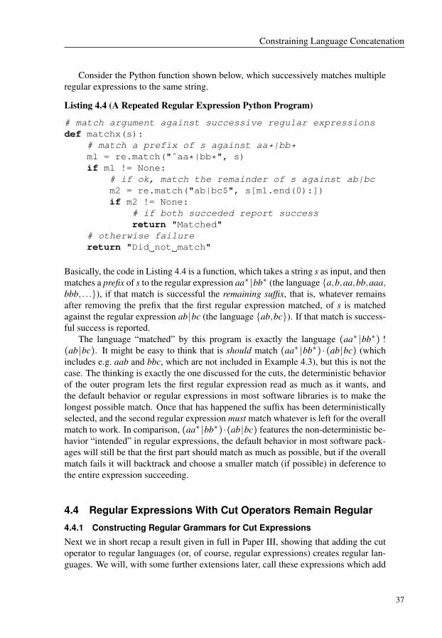
Constraining Language Concatenation
Consider the Python function shown below, which successively matches multipleregular expressions to the same string.
Listing 4.4 (A Repeated Regular Expression Python Program)
# match argument against successive regular expressionsdef matchx(s):
# match a prefix of s against aa*|bb*m1 = re.match("ˆaa*|bb*", s)if m1 != None:
# if ok, match the remainder of s against ab|bcm2 = re.match("ab|bc$", s[m1.end(0):])if m2 != None:
# if both succeded report successreturn "Matched"
# otherwise failurereturn "Did not match"
Basically, the code in Listing 4.4 is a function, which takes a string s as input, and thenmatches a prefix of s to the regular expression aa∗ ∣bb∗ (the language {a,b,aa,bb,aaa,bbb, . . .}), if that match is successful the remaining suffix, that is, whatever remainsafter removing the prefix that the first regular expression matched, of s is matchedagainst the regular expression ab ∣bc (the language {ab,bc}). If that match is success-ful success is reported.
The language “matched” by this program is exactly the language (aa∗ ∣bb∗) !(ab ∣bc). It might be easy to think that is should match (aa∗ ∣bb∗) ⋅ (ab ∣bc) (whichincludes e.g. aab and bbc, which are not included in Example 4.3), but this is not thecase. The thinking is exactly the one discussed for the cuts, the deterministic behaviorof the outer program lets the first regular expression read as much as it wants, andthe default behavior or regular expressions in most software libraries is to make thelongest possible match. Once that has happened the suffix has been deterministicallyselected, and the second regular expression must match whatever is left for the overallmatch to work. In comparison, (aa∗ ∣bb∗) ⋅(ab ∣bc) features the non-deterministic be-havior “intended” in regular expressions, the default behavior in most software pack-ages will still be that the first part should match as much as possible, but if the overallmatch fails it will backtrack and choose a smaller match (if possible) in deference tothe entire expression succeeding.
4.4 Regular Expressions With Cut Operators Remain Regular
4.4.1 Constructing Regular Grammars for Cut Expressions
Next we in short recap a result given in full in Paper III, showing that adding the cutoperator to regular languages (or, of course, regular expressions) creates regular lan-guages. We will, with some further extensions later, call these expressions which add
37
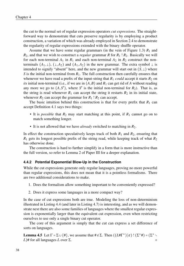
Chapter 4
the cut to the normal set of regular expression operators cut expressions. The straight-forward way to demonstrate that cuts preserve regularity is by employing a productconstruction, a variation of which was already employed in Section 2.4 to demonstratethe regularity of regular expressions extended with the binary shuffle operator.
Assume that we have some regular grammars (in the vein of Figure 1.3) R1 andR2, and that we wish to construct a regular grammar R for R1 ! R2. Basically we willfor each non-terminal A1 in R1 and each non-terminal A2 in R2 construct the non-terminals (A1,�), (�,A2) and (A1,A2) in the new grammar. The extra symbol � isintended to signify “absent” here, and the new grammar will start out in (S,�) whereS is the initial non-terminal from R1. The full construction then carefully ensures thatwhenever we have read a prefix of the input-string that R1 could accept it starts R2 onits initial non-terminal (i.e., if we are in (A,B) and R1 can get rid of A without readingany more we go to (A,S′), where S′ is the initial non-terminal for R2). That is, asthe string is read whenever R1 can accept the string it restarts R2 in its initial state,whenever R2 can accept the grammar for R1 ! R2 can accept.
The basic intuition behind this construction is that for every prefix that R1 canaccept Definition 4.1 says two things:
• It is possible that R2 may start matching at this point, if R1 cannot go on tomatch something longer.
• It is not allowed that we have already switched to matching in R2.
In effect the construction speculatively keeps track of both R1 and R2, ensuring thatR1 gets its longest possible prefix of the string read, while keeping track of what R2has otherwise done.
The construction is hard to further simplify in a form that is more instructive thanthe full version, so refer to Lemma 2 of Paper III for a deeper explanation.
4.4.2 Potential Exponential Blow-Up in the Construction
While the cut expressions generate only regular languages, proving no more powerfulthan regular expressions, this does not mean that it is a pointless formalisms. Thereare two additional considerations to make.
1. Does the formalism allow something important to be conveniently expressed?
2. Does it express some languages in a more compact way?
In the case of cut expressions both are true. Modeling the loss of non-determinismillustrated in Listing 4.4 (and later in Listing 4.7) is interesting, and as we will demon-strate next there are also some families of languages where the smallest regular expres-sion is exponentially larger than the equivalent cut expression, even when restrictingourselves to use only a single binary cut operator.
The core of this argument is simply that the cut can express a set difference ofsorts on languages.
Lemma 4.5 Let Γ = Σ∪{#}, we assume that # ∉ Σ. Then ((L#Γ∗)∣ε) ! (Σ∗#) = (Σ∗∖L)# for all languages L over Σ. ◇
38

Constraining Language Concatenation
A complete proof of this lemma is out of the scope of this introduction, but it is fairlyintuitive when one considers the cases. Assume that w ∈ L, then, for the lemma tohold, w# should not be in ((L#Γ∗)∣ε) ! Σ∗#. This is clearly the case, as the L#Γ∗ willconsume it entirely, leaving nothing for the trailing Σ∗# to match. This in fact holdsfor any string v with w# as a prefix, as the Γ∗ keeps consuming all symbols. In theother direction, assume that w ∉ L. Then w# is not matched by L#Γ∗, meaning that theε part of the branch is chosen, and then Σ∗# matches it and the match succeeds.
To exploit Lemma 4.5 we can now construct a regular expression R over Σ suchthat the shortest string R does not match is exponential in length (compared to thelength of R). We can then apply Lemma 4.5, taking L as L(R), to produce a cutexpression for which the shortest matching string is exponential in the length of theexpression. From this we can then draw the conclusion that the smallest regular gram-mar (or finite automaton or regular expression) is at least exponentially larger thanthe cut expression. Recall Definition 1.6 in preparation, and note that Rk (for someregular expression R and k ∈ N) is not a regular expression operator, but is here usedas an abbreviation for
R ⋅R⋯R´¹¹¹¹¹¹¹¹¹¸¹¹¹¹¹¹¹¹¹¶k times
.
If regular expressions are extended with an actual Rk operator the explosion in sizewould be even greater.
We select Σ = {0,1,$} as the alphabet, and let ∆ = {0,1}. For each n ∈N the regularexpression Rn has five components, Rn = A ∣B ∣Cn ∣Dn ∣En, which are as follows. In theend the language considered will be (Σ∗ ∖L(Rn))#, so the aspect to consider is e.g.the language Σ∗∖A and so on.
1. A = ∆Σ∗ ∣$∆∗1∆∗$Σ∗. Note that all strings in Σ∗∖A start with $ and contain no1 until the next $.
2. B = Σ∗∆ ∣Σ∗$∆∗0∆∗$. Note that all strings in Σ∗∖B end with $ and contain nozero between the last two $ symbols.
3. Cn = Σ∗$∆n+1∆∗$Σ∗ ∣Cn,0⋯Cn,n−1 where Cn,i = Σ∗$∆i$Σ∗ for each i. Note thatall strings in Σ∗ ∖Cn have exactly n zeroes and ones between each pair of $symbols.
4. Dn = Dn,1 ∣⋯ ∣Dn,n−2, where Dn,i = Σ∗$∆i0∆∗0∆∗$∆i1∆∗$Σ∗ for each i. Notethat the strings in Σ∗ ∖Dn are such that every substring $x$y$ (with x,y ∈ ∆n,which will be enforced by Cn), is such that if the ith symbol in x is a zero, andthe ith symbol in y is a 1, then symbols i+1 through n in x must be ones.
5. En = En,1 ∣⋯En,n−2 where En,i = Σ∗$∆i01n−i−1$∆i1∆∗1∆∗$Σ∗ for each i. Notethat all strings in Σ∗ ∖En are such that every substring $x$y$ (with x,y ∈ ∆n,which will be enforced by Cn), is such that if the ith symbol in x is a 0, symbolsi+1 through n are ones, and the ith symbol in y is a 1, then the remainder of ymust be zeroes.
39

Chapter 4
Taking all these together we learn that each w ∈ (Σ∗ ∖L(Rn)) are strings such thatw = $x1$x2$⋯$xm$ where each xi is a string of n zeroes and ones (due to Cn), such thatx1 = 0⋯0 (due to A), and xn = 1⋯1 (due to B). At most one zero in xi can be turned intoa one in xi+1, and only if all the subsequent positions were ones in xi and are zeroesin xi+1. From this it directly follows that the shortest string in Σ∗ ∖L(Rn) will be thesequence of all n-bit binary strings in order, for example
$000$001$010$011$100$101$110$111$ ∈ R3.
In addition a number of longer strings exist, which show up since a one in xi may turninto a zero in xi+1. However, the only way to get from the initial zero sequence to thefinal one sequence is to increment by one in the binary addition sense at least 2n times.
Notice, however, that the actual expression Rn is on the order of n2 symbols long,where Cn, Dn and En are the big part. Applying Lemma 4.5 constructs a cut expressionaccepting (Σ∗∖L(Rn))#, which is still on the order of n2 symbols long, but as arguedabove the shortest string it accepts is exponential in n.
Non-extended regular expressions, regular grammars (as sketched in figures here)and finite automata are all such that the shortest string they accept is at most linear inthe size of the expression/grammar/automaton (if they accept any string at all). Thisis easy to see, some efficient shortest path algorithm can be employed to find a paththrough the expression/grammar/automaton. As such, cut expressions are exponen-tially more succinct in some cases, and converting an arbitrary cut expression into oneof those listed formalisms may create an exponentially larger representation. This willbe rather key to understanding the complexity of solving the membership problem.
4.5 The Iterated Cut
In a further parallel with Chapter 2 we also consider a unary iterated version of thecut. Much like R⊙ = R⊙R⊙⋯⊙R we let R!∗ = R ! (R ! (R ! ⋯(R ! R)⋯)). However,notice that while the shuffle operator is associative, the cut operator is not.
Example 4.6 Let us consider two expressions differing only in associativity ((ab)∗ !a) ! b and (ab)∗ ! (a ! b).
• For ((ab)∗ ! a) ! b clearly (ab)∗ ! a is the same as (ab)∗a, since the (ab)∗part cannot cover the final a, so L((ab)∗ ! a) = {a,aba,ababa, . . .}, and, hence,L(((ab)∗ ! a) ! b) = {ab,abab,ababab, . . .}.
• However, if we instead consider (ab)∗ ! (a ! b), we notice that a ! b is the sameas ab, so we have (ab)∗ ! ab which is clearly empty, as the (ab)∗ will consumeall repetitions of ab ensuring the second part never gets to match anything.
It follows that the cut operator is not associative. ◇The iterated cut, in a sense similar to how the binary cut models the program in List-ing 4.4, permits the modeling of loops of regular expression matching, like in thebelow listing.
40

Constraining Language Concatenation
Listing 4.7 (A Looping Regular Expression Python Program)
# match s against the regular expression R repeatedlydef matchy(R, s):
# keep matchingwhile True:
# match s to re oncem = re.match(R, s)# if the match failed report failureif m == None:
return "Did not match"# otherwise, extract the remainder of the matchs = s[m.end(0):]# if the whole string matched, report successif len(s) == 0:
return "Matched"
This listing will give the same behavior as trying to match s to R!∗.The iterated cut is hard to express directly in a regular expression with just the
addition of the binary cut operator. Notably it is not a matter of nesting cuts inside ofKleene closures, like (R ! R)∗ or similar, as this will give too much non-deterministicfreedom in general. However, adding both the binary cut operator and the iteratedcut to regular expression still produces expressions that can only generate regular lan-guages. The construction for this part is slightly trickier than for the case of the binarycut operators, so it is best to refer to Paper III where complete and formal constructionsfor both cases are given.
4.6 Regular Expression Extensions, Impact and Reality
4.6.1 Lifting Operators to the Sets
Recall Definition 1.6 where the basic operations in regular expressions are defined. Itis an important fact to note that each of those classical regular expression operatorsare expressed string-wise. That is, an operator f takes n argument subexpressionsR1, . . . ,Rn, and the language it generates is then
L( f (R1, . . . ,Rn)) = { f (v1, . . . ,vn) ∣ v1 ∈ L(R1), . . . ,vn ∈ L(Rn)}.That is, the classic operators all operate “point-wise” on strings, and this is then liftedto the level of sets (i.e. we can take the categorial view and consider a functor here) togenerate languages. However, the cut does not operate on this level. Instead Defini-tion 4.1 operates on the level of the language. We can talk about L ! L′ for languages,but informed that w ∈ L and v ∈ L′ we cannot from this determine whether wv ∈ L ! L′.
This should be viewed as a flaw with the cuts, their introduction into expressionsdoes change the nature of the expression in a fundamental way. On the other hand,the impact is comparatively small when contrasted to the cut-like operators that many
41

Chapter 4
regular expression software packages include. These have behavior that is even furtherfrom the clean nature of the classical operators.
4.6.2 An Aside: Regular Expression Matching In Common Software
This way of phrasing how matching happens may appear unusual for anyone more fa-miliar with the more classic regular expression constructions, where the semantics aredescribed in a composed way, i.e., L(R1 ∣R2) = L(R1)∪L(R2), etc., or by construct-ing finite automata for the expression (constructing the Glushkov automaton [Glu61]and determinising it, or directly constructing a deterministic finite automaton usinge.g. derivatives [Brz64]). Most practical software packages, however, use a depth-first backtracking search across some abstract syntax tree representation of the regularexpression. The reasons for this are two-fold.
1. The efficiency of this approach is in many cases great. Constructing the syntaxtree is efficient, and the representation is in general far more compact than theautomata approach. The actual search may in the worst case be a lot slower(exponential in the length of the string), but the semantics are straightforwardenough that the task of structuring the expression in a way that gives efficientmatching in the most common cases can be left to the programmer.
2. It enables a multitude of additional regular expression features. Most immedi-ately it makes it possible to deterministically talk about which part of the regularexpression matches which part of the string. That is, (a∗ ∣b∗)(a ∣b)∗ matchesaaababa, but which part of the expression matches the aaa prefix? In the the-oretical setting this is a nonsense question, all we state is that aaababa ∈ L , thehow is entirely undefined. In regular expression software packages however theinitial three as will be matched by the first a∗, and this information can be ex-tracted with the API provided. Which parts of the expression will “prefer” tomatch what can be controlled further with a variety of operators, and the piecesof the string matched by a certain subexpression can even be recalled inside theexpression (permitting the language {ww ∣ w ∈ Σ∗} to be matched by recalling acopy of the string already matched).
In short; the accepted approach has numerous implications for the functionality andperformance of regular expression matching in practice.
4.6.3 Real-World Cut-Like Operators
There are a variety of operators in practical regular expression packages which behavesomewhat similar to cuts. The first, and most common, are the possessive quantifiers.Let us look specifically at the possessive variation of the Kleene star R∗ as defined inDefinition 1.6, denoted R∗+. Defining the language generated by R∗+ leads to disap-pointment however, L(R∗+) = {ε}∪{vw ∣ v ∈L(R),w ∈L(R∗+)} inductively. Unfortu-nately this is precisely the same language as generated by L(R∗), which is because thepossessive quantifier does not operate on the same level as classical regular operators,or even the set-level behavior of the cut operators. Instead the semantics of the posses-sive quantifiers are intertwined with the overall matching of the entire expression in a
42

Constraining Language Concatenation
way that is hard to formalize. Consider the examples in Table 4.8 which are producedusing the Java (1.6.0u18) regular expression implementation. Notice how applying
Table 4.8: Some regular expressions using possessive quantifiers and the languagethey accept in Java 1.6.0u18.
Expression Language(aa)∗+a {a,aaa,aaaaa,aaaaaaa, . . .}((aa)∗+a)∗ {ε,a,aaa,aaaaa,aaaaaaa, . . .}((aa)∗+a)∗a {a}the Kleene star to the expression in the first row does not (in the second row) generatefor example aa, despite a being in the language of the first row.
We will not attempt to deeply explain the semantics of this operator, but it operatesby manipulating the internal backtracking search. The outcome does not easily fit intothe compositional classic explanation of how regular expressions generate languages.See Paper III for more examples of this type of operator.
As an addition, some regular expression engines feature an additional binary op-erator, (*PRUNE), that compares fairly directly to the binary cut operator (in that itis not attached to a Kleene star), but still has semantics that are hard to comprehendform the compositional perspective. See Table 4.9 for some examples of expressionsand the languages recognized in Perl 5.16.2.
Table 4.9: Some regular expressions using the (*PRUNE) operator and the languagethey accept in Perl 5.16.2, similar to the examples in Table 4.8.
Expression Language(aa)∗(*PRUNE)a {a,aaa,aaaaa,aaaaaaa, . . .}((aa)∗(*PRUNE)a)∗ ∅((aa)∗(*PRUNE)a)∗a ∅
4.6.4 Exploring Real-World Regular Expression Matchers
Paper IV explores the behavior of these practical software package matchers. Theyeffectively operate by constructing an automaton (or grammar) where rules are prior-itized, whenever there are multiple rules that could be applied there is a preferred rulethat is tried first. If applying that rule does not lead to accepting the string the proce-dure backtracks and tries the other options. The full discussion requires a deep tech-nical look at the behavior of the software, and is best explored by reading Paper IV.Suffice it to say, beyond exploring the semantics to analyze additional operators, thissearch procedure will additionally at times require exponential time. Consider for ex-
43
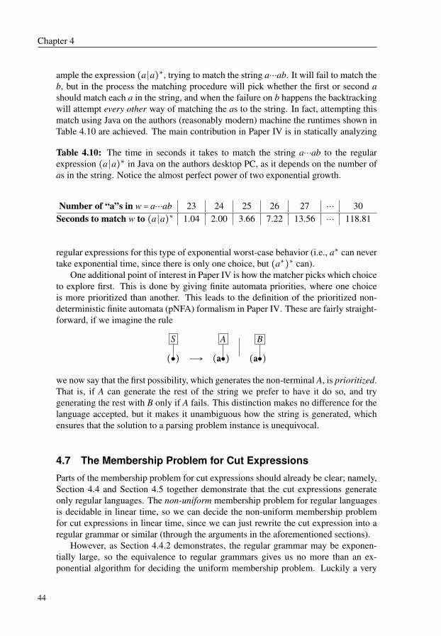
Chapter 4
ample the expression (a ∣a)∗, trying to match the string a⋯ab. It will fail to match theb, but in the process the matching procedure will pick whether the first or second ashould match each a in the string, and when the failure on b happens the backtrackingwill attempt every other way of matching the as to the string. In fact, attempting thismatch using Java on the authors (reasonably modern) machine the runtimes shown inTable 4.10 are achieved. The main contribution in Paper IV is in statically analyzing
Table 4.10: The time in seconds it takes to match the string a⋯ab to the regularexpression (a ∣a)∗ in Java on the authors desktop PC, as it depends on the number ofas in the string. Notice the almost perfect power of two exponential growth.
Number of “a”s in w = a⋯ab 23 24 25 26 27 ⋯ 30Seconds to match w to (a ∣a)∗ 1.04 2.00 3.66 7.22 13.56 ⋯ 118.81
regular expressions for this type of exponential worst-case behavior (i.e., a∗ can nevertake exponential time, since there is only one choice, but (a∗)∗ can).
One additional point of interest in Paper IV is how the matcher picks which choiceto explore first. This is done by giving finite automata priorities, where one choiceis more prioritized than another. This leads to the definition of the prioritized non-deterministic finite automata (pNFA) formalism in Paper IV. These are fairly straight-forward, if we imagine the rule
(●●)S
Ð→ (aa●●)A
(aa●●)B
we now say that the first possibility, which generates the non-terminal A, is prioritized.That is, if A can generate the rest of the string we prefer to have it do so, and trygenerating the rest with B only if A fails. This distinction makes no difference for thelanguage accepted, but it makes it unambiguous how the string is generated, whichensures that the solution to a parsing problem instance is unequivocal.
4.7 The Membership Problem for Cut Expressions
Parts of the membership problem for cut expressions should already be clear; namely,Section 4.4 and Section 4.5 together demonstrate that the cut expressions generateonly regular languages. The non-uniform membership problem for regular languagesis decidable in linear time, so we can decide the non-uniform membership problemfor cut expressions in linear time, since we can just rewrite the cut expression into aregular grammar or similar (through the arguments in the aforementioned sections).
However, as Section 4.4.2 demonstrates, the regular grammar may be exponen-tially large, so the equivalence to regular grammars gives us no more than an ex-ponential algorithm for deciding the uniform membership problem. Luckily a very
44

Constraining Language Concatenation
direct table parsing algorithm can decide membership in cubic time. Let us sketchvery quickly how it is done.
Algorithm 4.11 (Parsing for Cut Expressions) Take as input a cut expression E anda string α1⋯αn. Let SE denote the set of subexpressions of E (including E itself).
1: Construct the table T ∶ SE ×{1, . . . ,n+1}×{1, . . . ,n+1}→ {true, false}.2: Set T(E, i, j) ∶= false for all E, i, j at the start3: for S ∈ SE , working bottom-up through the sub-expressions do4: if S = ε then T(S, i, i) ∶= true5: else if S ∈ Σ then T(S, i, i+1) ∶= true for all i with αi = S6: else if S = E1 ∣E2 then7: T(S, i, j) ∶= true for all i ≤ j s.t. T(E1, i, j)∨T(E2, i, j)8: else if S = E1 ⋅E2 then9: T(S, i,k) ∶= true for all i ≤ j ≤ k s.t. T(E1, i, j)∧T(E2, j,k)
10: else if S = E∗1 then
11: T(S, i1, in) ∶= true for all n, i1 ≤⋯ ≤ in s.t. T(E1, i1, i2)∧⋯∧T(E1, in−1, in)12: else if S = E1 ! E2 then13: T(S, i,k) for all i ≤ j ≤ k such that:14: T(E1, i, j)∧T(E2, j,k), and,15: ¬T(E1, i, j′) for all j < j′ ≤ k.16: end if17: end for
This algorithm is trivially cubic (quadratic in the length of the string), since everytable position is set true at most once. The case for the shuffle closure is not included,but is a trivial addition.
After the threat of potentially exponentially large regular grammars the cubic time(and space) of the above algorithm may be calming, but given the typical efficiency ofmatching classical regular expressions cubic time is still not entirely pleasing. Betteralgorithms remain an open question however, very notably Section 4.4.2 demonstratesa case where applying a cut exponentially blows up the size of the smallest corre-sponding regular grammar exponentially, but for the upper bound we only know thatit cannot be worse than non-elementary, which is not very satisfying. This in fact fol-lows from the product-style construction discussed in Section 4.4.1, and is discussedat greater length in Paper III.
45
Chapter 4
46

CHAPTER 5
Block Movement Reordering
This short chapter discusses matters of block reordering, which is once again a non-obvious term, this time lifted form the field of edit distance, where operations thatmodify multiple symbols in a contiguous substring at once are referred to as blockoperations. Specifically the topic of interest is attempting to study the results of re-ordering nodes in the parse tree for a string, which gives rise to a sort of hierarchicalblock movement reordering in the underlying string language.
5.1 String Edit Distance
String edit distance is a long studied field. It is concerned with defining a distancebetween strings using a sequence of operations (reminiscent of the rule-based deriva-tions discussed in earlier chapters, but starting from another, possibly longer, string).The distance measure is defined in terms of a set of operations, each of which makessome small modification to a string, and then the distance between a string w ∈ Σ∗and v ∈ Σ∗ is the minimum number of operations (possibly weighted in some way) weneed to apply to modify w into v. The problem of finding this sequence is known as thestring correction problem. A classic set of operations for this is to have an operationto delete a single symbol and one to insert a single symbol. Making the distance frome.g. abc to cca four, since the initial ab must be removed (two removal operations)and ca must be added at the end. A typical additions to the set of operations is toadd an operator to replace one symbol by another, this set of three operators is calledLevenshtein distance [Lev66]. The next typical addition, and most important for ushere, is the swap, which swaps the positions of two adjacent symbols, the resulting setof operators is called Damerau-Levenshtein distance [Dam64].
5.2 A Look at Error-Dilating a Language
The direction of interest here starts out from the question of an error dilation of alanguage. Consider Figure 5.1. That is, we choose a language class G (perhaps theregular or context-free languages) and a string edit distance e, then for each languageL ∈ G and each k ∈ N we define Le=k to mean that w ∈ Le=k if and only if there existssome v ∈ L such that w is k or less distance from v. Notably, as k approaches ∞ the
47
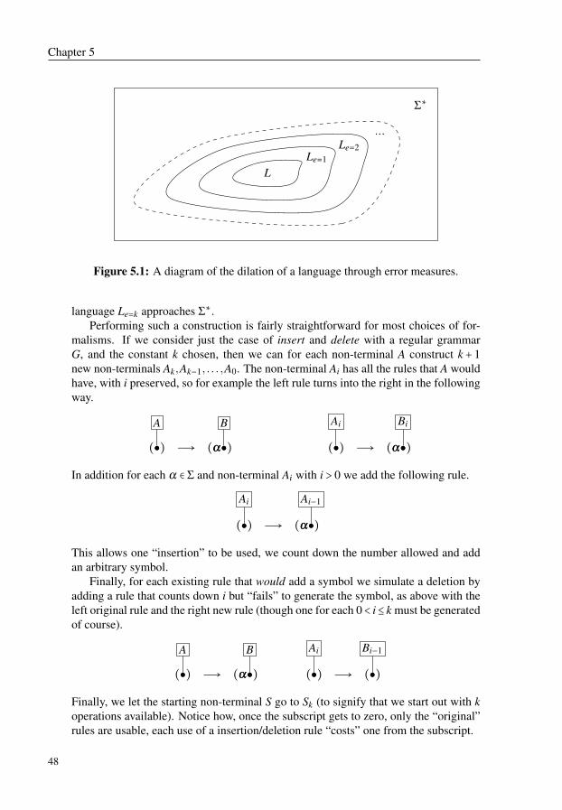
Chapter 5
Σ∗
LLe=1
Le=2⋯
Figure 5.1: A diagram of the dilation of a language through error measures.
language Le=k approaches Σ∗.Performing such a construction is fairly straightforward for most choices of for-
malisms. If we consider just the case of insert and delete with a regular grammarG, and the constant k chosen, then we can for each non-terminal A construct k+ 1new non-terminals Ak,Ak−1, . . . ,A0. The non-terminal Ai has all the rules that A wouldhave, with i preserved, so for example the left rule turns into the right in the followingway.
(●●)A
Ð→ (αα●●)B
(●●)Ai
Ð→ (αα●●)Bi
In addition for each α ∈ Σ and non-terminal Ai with i > 0 we add the following rule.
(●●)Ai
Ð→ (αα●●)Ai−1
This allows one “insertion” to be used, we count down the number allowed and addan arbitrary symbol.
Finally, for each existing rule that would add a symbol we simulate a deletion byadding a rule that counts down i but “fails” to generate the symbol, as above with theleft original rule and the right new rule (though one for each 0< i≤ k must be generatedof course).
(●●)A
Ð→ (αα●●)B
(●●)Ai
Ð→ (●●)Bi−1
Finally, we let the starting non-terminal S go to Sk (to signify that we start out with koperations available). Notice how, once the subscript gets to zero, only the “original”rules are usable, each use of a insertion/deletion rule “costs” one from the subscript.
48
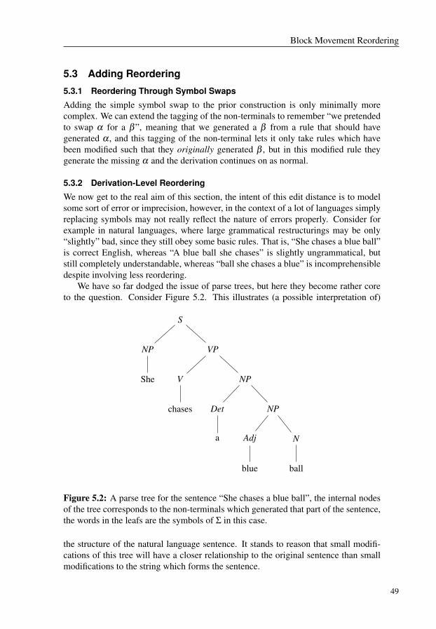
Block Movement Reordering
5.3 Adding Reordering
5.3.1 Reordering Through Symbol Swaps
Adding the simple symbol swap to the prior construction is only minimally morecomplex. We can extend the tagging of the non-terminals to remember “we pretendedto swap α for a β”, meaning that we generated a β from a rule that should havegenerated α , and this tagging of the non-terminal lets it only take rules which havebeen modified such that they originally generated β , but in this modified rule theygenerate the missing α and the derivation continues on as normal.
5.3.2 Derivation-Level Reordering
We now get to the real aim of this section, the intent of this edit distance is to modelsome sort of error or imprecision, however, in the context of a lot of languages simplyreplacing symbols may not really reflect the nature of errors properly. Consider forexample in natural languages, where large grammatical restructurings may be only“slightly” bad, since they still obey some basic rules. That is, “She chases a blue ball”is correct English, whereas “A blue ball she chases” is slightly ungrammatical, butstill completely understandable, whereas “ball she chases a blue” is incomprehensibledespite involving less reordering.
We have so far dodged the issue of parse trees, but here they become rather coreto the question. Consider Figure 5.2. This illustrates (a possible interpretation of)
S
NP
She
VP
V
chases
NP
Det
a
NP
Adj
blue
N
ball
Figure 5.2: A parse tree for the sentence “She chases a blue ball”, the internal nodesof the tree corresponds to the non-terminals which generated that part of the sentence,the words in the leafs are the symbols of Σ in this case.
the structure of the natural language sentence. It stands to reason that small modifi-cations of this tree will have a closer relationship to the original sentence than smallmodifications to the string which forms the sentence.
49

Chapter 5
5.3.3 Tree Edit Distance
Tree edit distance is a natural way to think about this, that is, we would like to createan error dilation of a language, in the style of Figure 5.1 using tree operations on theparse tree (which requires a specific instance of a grammar for the language to makesense) to modify the final strings.
The problem of tree edit distance is fairly well explored in some limited settings,see e.g. [Sel77, Tai79]. This work has for the most part however been constrainedto just allowing insert and delete operators, the swap, or similar subtree movementoperators, is a trickier matter [ZS89, Kle98, Bil05]. This is partially necessary, thetree edit distance on unordered trees (i.e., we allow deletions and insertions of nodes,but siblings in the tree have no order) is NP-complete [ZSS92]. We can simulatethe unordered case if swaps are permitted, by simply replacing each internal node bya long chain of copies of the node. This way the swap remains cheap (it does notcare how many nodes it moves in swapping two siblings) while making insertions anddeletions expensive. If we add sufficiently many of these nodes the result will be thatall orders can be achieved cheaper than it is to perform a single insertion or deletion,effectively making the problem behave like the unordered case.
5.4 Analyzing the Reordering Error Measure☆Paper VI considers the very limited case of only permitting tree swaps in the distancemeasure, each swap having a cost of one. Let us consider the proper definition, re-calling the definitions of trees from Section 2.9.1. First we define the swap distancebetween permutations.
Definition 5.3 Let πn ⊂Nn denote the set of permutations of length n, that is, p1⋯pn ∈πn if and only if {p1, . . . , pn} = {1, . . . ,n}. Then p1⋯pn ∈ πn has a swap distance lessthan or equal to k, denoted swap(p1⋯pn,k) if and only if
• k ≥ 0 and p1⋯pn = 1⋯n,
• there exists some i such that swap(p1⋯pi−1 pi+1 pi pi+2⋯pn,k−1). ◇Then the tree variant is as follows.
Definition 5.4 For two trees t,t′ we say that t and t′ are within tree swap distancek, denoted swap(t,t′,k), if and only if t = α[t1, . . . ,tn] and t′ = α[t′1, . . . ,t′n] for someα ∈ Σ and n, and there exists some p1⋯pn ∈ πn and l0, . . . , ln ∈N such that
• k ≥∑ni=0 li,
• swap(p1⋯pn, l0), and
• swap(ti,tpi , li) for all i.
The triple (t,t′,k) is a “yes” instance of the tree swap distance problem if and onlyif swap(t,t′,k). ◇
50

Block Movement Reordering
Unfortunately this problem is proven to be NP-hard in Paper VI (the problem is ob-viously in NP, since the permutations for each level of the tree can be guessed andthen verified in polynomial time). Let us briefly outline the process. The reductionstarts with the extended string-to-string correction problem, which is an edit distancewith only delete and swap operations1. This problem is known to be NP-complete(see e.g. [GJ90]). The reduction makes an intermediary stop in a problem that may beinteresting in itself.
Definition 5.5 Let M ∶ N×N → N be an n by n matrix (i.e. a matrix with n rowsand columns, letting M(i, j) denote the value at the ith row and jth column), then(M,k) is a “yes” instance of the swap assignment problem if and only if there exists apermutation p1⋯pn ∈ πn and l ∈N such that
• swap(p1⋯pn, l)• k ≥ l+∑n
i=1 M(pi, i) ◇That is, the problem is to decide whether it is possible to swap rows positions in M insuch a way that the sum of the number of swaps used and the diagonal in the resultingmatrix is less than or equal to k. The reduction is such that e.g. position M(i, j) iszero if symbol i of the first string in the original edit distance problem is the same assymbol j in the second, combined with some trickery to enable deletions.
This matrix problem is then in turn reduced to the tree swap problem of Defini-tion 5.4. This reduction is not overly difficult, the tree constructed will have height3, the root has n immediate children corresponding to the rows, these have n childrencorresponding to the column positions in that row, and finally these have a codingof the number they should contain as children. Everything is distinctly coded so theswaps can only be used to reorder the rows, and to make the binary representationsequal (which costs exactly the absolute difference between the numbers).
The fact that the tree swap distance is NP-complete is unfortunate, however, theamount of distance permitted in the error-dilating of languages should be very con-strained (e.g. a sentence with three or more errors will often be incomprehensiblealready), so fixed parameter analysis and other more nuanced analysis would be ofgreat interest.
1 This statement abuses the notion of a distance heavily, since it is asymmetric. It does however fall intoa similar class of problems.
51

Chapter 5
52

CHAPTER 6
Summary and Loose Ends
None of the matters here can be considered settled or treated with some deep finality.This is a snapshot of ongoing research, here tied together with an overarching theme,but it is both likely and desirable that everything here treated will be supplanted withnew greater results in the future. As such this concluding chapter attempts to lookforward, while and noting the missing pieces, as well as summarizing some of theaspects of the attached papers that have not yet been brought up.
6.1 Open Questions and Future Directions
6.1.1 Shuffle Questions
There are two open questions from the preceding licentiate thesis [Ber12] that may beinteresting to recall.
1. Deciding the membership problem for the shuffle of palindromes:
{wwR ∣ w is any string, wR is w reversed}.2. Deciding the membership problem for the language of shuffle squares,
{w⊙w ∣ w is any string}.Notice that as the languages we are concerned with are specified as part of the problemthese should be viewed as non-uniform membership problems.
The first remains a point of interest, Paper I demonstrates that the non-uniformmembership problem for two linear deterministic context-free languages is NP-hard(see Chapter 2), and the shuffle of two palindromes seems like, in a spirit rather similarto the ideas of Paper V, or possibly more illustratively the Chomsky-Schutzenbergertheorem [CS63], the next step. That is, the palindromes are sort of the most primitiverepresentation of the basic power that differentiates the linear deterministic context-free languages from the regular, in that both the intersection and homomorphism inthe Chomsky-Schutzenberger decomposition of it do “nothing”. The author has nospeculation whether this problem should be expected to be in P or not.
The shuffle square, on the other hand, has seen some important developmentssince [Ber12], and is proven NP-complete in a rather tricky reduction in [BS13].
53

Chapter 6
In addition, let us note that the problems as stated above deal with languages witharbitrarily large alphabets (i.e., when it says that w is any string it may be over analphabet up to ∣w∣ in size). The reduction in [BS13] works for a finite alphabet versionof the shuffle square as well, meaning that the language is NP-complete either way.No results are known for the palindrome shuffle, so a possibility is that the problem isNP-complete for arbitrarily large alphabets, but is in P for all alphabet sizes smallerthan some constant.
Beyond that, there are numerous additional problems that may be considered inshuffle, especially as many aspects are of practical interest. Beyond simply improvingon many of the results in Paper I, and considering both more generalized and restrictedcases (shuffle on trajectories is a lively and interesting case), the problem the authormost wants to highlight is the one considered in Paper V. That is, proving that forall context-free languages L ⊆ Σ∗ and L′ ⊆ Γ∗ (with Σ∩Γ = ∅) the shuffle L⊙L′ iscontext-free if and only if one of L and L′ is regular.
6.1.2 Synchronized Substrings Questions
The synchronized substrings formalisms, such as linear context-free rewriting sys-tems, are a prime example of where the details of parsing complexity are hugely im-portant. The uniform membership algorithm appears inefficient from the classicalcomplexity theory perspective, but in practice the algorithms are considered reason-ably efficient (recall Section 3.4.3). Paper II does find some potentially efficient cases,but they are not necessarily entirely satisfactory, as the one truly efficient case iden-tified is where the rank, fan-out and derivation length are included in the parameter(i.e., if all three are small the parsing problem is efficient).
The most obvious case not yet studied is to take the opposite approach from theclassical non-uniform membership problem1; we let the length of the string be theparameter and consider the grammar in full, or near full. To see the reasoning herethe intended application may need to be clarified. These formalisms are typicallyused for natural language processing. In this case it is easy to see that the sizes ofthe components are backwards from what is usually assumed, the strings are simplynatural language sentences, and, while they can be long, like this run-on sentence,there are still very real practical limits on how many words there can be in one. Areasonably complete grammar for English however is vast at the best of times, simplyenumerating exceptions will create tens of thousands of rules. As such the complexityin the grammar is actually more important than the complexity in the string.
6.1.3 Regular Expression Questions
The two Papers III and IV both deal with very similar issues, in that they are motivatedby the order-dependencies that exist in practical regular expression semantics as aneffect of matching methodology employed. Their approaches are very different how-
1 Notice however, here we talk about parameterized complexity, the intent is not to clumsily assume someparts constant like in the non-uniform case. Parameterized complexity bounds still take the parts put inthe “parameter” into account, but differentiate between how large a role that part plays in the complexity.See Section 3.5.1.
54
Summary and Loose Ends
ever, in that Paper III attempts to bring an approximation (attempting to make thembehave nicely within the classical framework) of these effects into a formal frame-work, whereas Paper IV tries to analyze the actual state of being of these regular ex-pression engines using formal techniques. The way forward here is not immediatelyobvious, there are clear open questions that follow directly from Paper III (e.g. an up-per bound on the automaton size), as well as some mechanical improvements alreadyconsidered. On the other hand Paper IV having a continuation is to a great extent aquestion of impact, as the paper may very well inspire changes in regular expressionengines, which would make continued research chase a moving target. A possibilitywhich has both advantages and disadvantages.
As such there is a wealth of possible work in the area of regular expression se-mantics, but beyond incremental open questions which are already listed in the papersthemselves this direction depends on the expected and actual impact of the research.
6.1.4 Other Questions
Paper V is obviously a work in progress published primarily for inclusion in this thesis.The conjecture presented does, however, appear very promising and significant, farbeyond proving the open question for context-free shuffles discussed above. In theother direction, Paper VI is the oldest paper included, and is concerned with a directionthat has not gotten a high level of attention from the author since. Continuing workappears to be a matter of extending the discussion in Chapter 5 in a way that arrives at areasonably compelling language class, while having clearly motivated fixed parametercomplexity problem with a positive outcome.
6.2 Conclusion
As a final remark the author wishes to again thank all his collaborators and colleagues,as well as everyone who worked on the many pieces of research leveraged as prelimi-naries in this work. Finally, the author thanks the reader for the interest shown.
55

56

References
[Bar85] G. Edward Barton. On the complexity of ID/LP parsing 1. Computa-tional Linguistics, 11(4):205–218, 1985.
[BBB13] Martin Berglund, Henrik Bjorklund, and Johanna Bjorklund. Shuffledlanguages – representation and recognition. Theoretical Computer Sci-ence, 489-490:1–20, 2013.
[BBD13a] Martin Berglund, Henrik Bjorklund, and Frank Drewes. On the param-eterized complexity of Linear Context-Free Rewriting Systems. In Pro-ceedings of the 13th Meeting on the Mathematics of Language (MoL13), pages 21–29, Sofia, Bulgaria, August 2013. Association for Com-putational Linguistics.
[BBD+13b] Martin Berglund, Henrik Bjorklund, Frank Drewes, Brink van derMerwe, and Bruce Watson. Cuts in regular expressions. In Marie-PierreBeal and Olivier Carton, editors, Proceeding of the 17th InternationalConference on Developments in Language Theory (DLT 2013), pages70–81, 2013.
[BDvdM14] Martin Berglund, Frank Drewes, and Brink van der Merwe. Analyzingcatastrophic backtracking behavior in practical regular expression match-ing. Submitted to the 14th International Conference on Automata andFormal Languages (AFL 2014), 2014.
[Ber11] Martin Berglund. Analyzing edit distance on trees: Tree swap distanceis intractable. In Jan Holub and Jan Zdarek, editors, Proceedings of thePrague Stringology Conference 2011, pages 59–73. Prague StringologyClub, Czech Technical University, 2011.
[Ber12] Martin Berglund. Complexities of Parsing in the Presence of Reordering.Licentiate thesis, Umea University, 2012.
[Ber14] Martin Berglund. Characterizing non-regularity. Technical ReportUMINF 14.12, Computing Science, Umea University, http://www8.cs.umu.se/research/uminf/, 2014. In collaboration with Hen-rik Bjorklund and Frank Drewes.
[Bil05] Philip Bille. A survey on tree edit distance and related problems. Theor.Comput. Sci., 337(1-3):217–239, 2005.
57
References
[BN01] Eberhard Bertsch and Mark-Jan Nederhof. On the complexity of someextensions of rcg parsing. In IWPT, 2001.
[Bou98] Pierre Boullier. Proposal for a Natural Language Processing SyntacticBackbone. Research Report RR-3342, INRIA, 1998.
[Bou04] Pierre Boullier. Range concatenation grammars, pages 269–289. KluwerAcademic Publishers, Norwell, MA, USA, 2004.
[Brz64] Janusz Brzozowski. Derivatives of regular expressions. Journal of theACM (JACM), 11(4):481–494, 1964.
[BS13] Sam Buss and Michael Soltys. Unshuffling a square is np-hard. Journalof Computer and System Sciences, 2013.
[CS63] Noam Chomsky and Marcel Paul Schutzenberger. The Algebraic Theoryof Context-Free Languages. In P. Braffort and D. Hirshberg, editors,Computer Programming and Formal Systems, Studies in Logic, pages118–161. North-Holland Publishing, Amsterdam, 1963.
[Dam64] Fred J. Damerau. A technique for computer detection and correction ofspelling errors. Commun. ACM, 7(3):171–176, 1964.
[DHK97] Frank Drewes, Annegret Habel, and Hans-Jorg Kreowski. Hyperedge re-placement graph grammars. In G. Rozenberg, editor, Handbook of GraphGrammars and Computing by Graph Transformation. Vol. 1: Founda-tions, chapter 2, pages 95–162. World Scientific, 1997.
[EB98] Zoltan Esik and Michael Bertol. Nonfinite axiomatizability of the equa-tional theory of shuffle. Acta Informatica, 35(6):505–539, 1998.
[FG06] Jorg Flum and Martin Grohe. Parameterized Complexity Theory.Springer-Verlag, 2006.
[Gaz88] Gerald Gazdar. Applicability of indexed grammars to natural languages.In Uwe Reyle and Christian Rohrer, editors, Natural Language Parsingand Linguistic Theories. Reidel Dordrecht, 1988.
[Gis81] Jay L. Gischer. Shuffle languages, Petri nets, and context-sensitive gram-mars. Communications of the ACM, 24(9):597–605, 1981.
[GJ90] Michael R. Garey and David S. Johnson. Computers and Intractability;A Guide to the Theory of NP-Completeness. W. H. Freeman & Co., NewYork, NY, USA, 1990.
[Glu61] Victor Michailowitsch Glushkov. The abstract theory of automata. Rus-sian Mathematical Surveys, 16(5):1–53, 1961.
[Got08] Daniel Norbert Gotzmann. Multiple context-free grammars. Technicalreport, Universitat des Saarlandes, 2008.
58

References
[GS65] Seymour Ginsburg and Edwin H. Spanier. Mappings of languages bytwo-tape devices. J. ACM, 12:423–434, July 1965.
[Hab92] Annegret Habel. Hyperedge Replacement: Grammars and Languages,volume 643 of Lecture Notes in Computer Science. Springer, 1992.
[HMU03] J. E. Hopcroft, R. Motwani, and J. D. Ullman. Introduction to AutomataTheory, Languages, and Computation (2nd Ed.). Pearson Education In-ternational, 2003.
[JLT75] Aravind K. Joshi, Leon S. Levy, and Masako Takahashi. Tree adjunctgrammars. J. Comput. Syst. Sci., 10(1):136–163, 1975.
[Jos85] Aravind K. Joshi. Tree adjoining grammars: How much context-sensitivity is required to provide reasonable structural description? Nat-ural Language Processing — Theoretical, Computational and Psycho-logical Perspective, 1985.
[JS01] Joanna Jedrzejowicz and Andrzej Szepietowski. Shuffle languages are inP. Theorical Computer Science, 250(1-2):31–53, 2001.
[JSW90] Aravind K. Joshi, K. Vijay Shanker, and David J. Weir. The convergenceof mildly context-sensitive grammar formalisms, 1990.
[Kle98] Philip N. Klein. Computing the edit-distance between unrooted orderedtrees. In In Proceedings of the 6th annual European Symposium on Al-gorithms (ESA, pages 91–102. Springer-Verlag, 1998.
[KNSK92] Y. Kaji, R. Nakanisi, H. Seki, and T. Kasami. The universal recogni-tion problem for multiple context-free grammars and for linear context-free rewriting systems. IEICE Transactions on Information and Systems,E75-D(1):78–88, 1992.
[Lev66] Vladimir I Levenshtein. Binary codes capable of correcting deletions,insertions, and reversals. Soviet Physics Doklady, 10(8):707–710, 1966.
[LW87] Klaus-Jorn Lange and Emo Welzl. String grammars with disconnect-ing or a basic root of the difficulty in graph grammar parsing. DiscreteApplied Mathematics, 16:17–30, 1987.
[MRS98] Alexandru Mateescu, Grzegorz Rozenberg, and Arto Salomaa. Shuf-fle on trajectories: syntactic constraints. Theoretical Computer Science,197(1-2):1–56, 1998.
[MS94] Alain J. Mayer and Larry J. Stockmeyer. Word problems – this time withinterleaving. Information and Computation, 115:293–311, 1994.
[ORR78] William F. Ogden, William E. Riddle, and William C. Rounds. Com-plexity of expressions allowing concurrency. In Proceedings of the 5thACM SIGACT-SIGPLAN symposium on Principles of programming lan-guages, POPL ’78, pages 185–194, New York, NY, USA, 1978. ACM.
59
References
[Pol84] Carl Pollard. Generalized phrase structure grammars, head grammarsand natural language. PhD thesis, Stanford University, 1984.
[Sel77] Stanley M. Selkow. The tree-to-tree editing problem. Inf. Process. Lett.,6(6):184–186, 1977.
[Sha78] Alan C. Shaw. Software descriptions with flow expressions. IEEE Trans.Softw. Eng., 4:242–254, May 1978.
[SMFK91] Hiroyuki Seki, Takashi Matsumura, Mamoru Fujii, and Tadao Kasami.On multiple context-free grammars. Theor. Comput. Sci., 88(2):191–229,October 1991.
[Ste87] Mark Steedman. Combinatory Grammars and Parasitic Gaps. NaturalLanguage and Linguistic Theory, 5:403–439, 1987.
[Tai79] Kuo-Chung Tai. The tree-to-tree correction problem. J. ACM, 26:422–433, July 1979.
[VdlC02] Eric Villemonte de la Clergerie. Parsing mildly context-sensitive lan-guages with thread automata. In Proceedings of the 19th internationalconference on Computational linguistics - Volume 1, COLING ’02, pages1–7, Stroudsburg, PA, USA, 2002. Association for Computational Lin-guistics.
[Wei88] David J. Weir. Characterizing mildly context-sensitive grammar for-malisms. Graduate School of Arts and Sciences, University of Penn-sylvania, 1988.
[Wei92] David J. Weir. Linear context-free rewriting systems and deterministictree-walking transducers. In Proceedings of the 30th annual meetingon Association for Computational Linguistics, ACL ’92, pages 136–143,Stroudsburg, PA, USA, 1992. Association for Computational Linguis-tics.
[WH84] Manfred K. Warmuth and David Haussler. On the complexity of iteratedshuffle. J. Comput. Syst. Sci., 28(3):345–358, 1984.
[ZS89] K. Zhang and D. Shasha. Simple fast algorithms for the editing distancebetween trees and related problems. SIAM J. Comput., 18(6):1245–1262,1989.
[ZSS92] Kaizhong Zhang, Rick Statman, and Dennis Shasha. On the editing dis-tance between unordered labeled trees. Information Processing Letters,42(3):133 – 139, 1992.
60

Umea University, SE-901 87 Umea, SwedenDepartment of Computing Science
www.cs.umu.se
ISBN 978-91-7601-047-1ISSN 0348-0542UMINF 14.13


