Complexity reduction in HEVC intra coding and comparison with

H.264/AVC

Vinoothna GajulaElectrical Engineering Graduate Student

The University of Texas at Arlington, 2013

Supervising Professor

K. R. Rao , EE Dept, UTACommittee Members

Dr. Kambiz Alavi , EE Dept, UTA

Dr. Russell Howard , EE Dept, UTA

AGENDA• Objective• Why compression?• History of video codecs• Introduction to HEVC• Overview of HEVC intra coding• Comparison between HEVC and H.264/AVC• Proposed fast intra prediction• Experimental results• Conclusion• Future research • References

OBJECTIVE

OBJECTIVEThe objective of this thesis is reducing the complexity of HEVC to get

better compression time, this is achieved by:

1. Reducing PU (prediction unit) size decision process using texture

complexity analysis by intensity gradient of image.

2. Obtaining the best prediction mode by applying a combination of

rough mode decision (RMD) and most probable modes (MPM)

reducing the number of modes to RDO followed by residual quad-tree

(RQT) checking is used to simplify the entire process.

Why compression?

Why compression?• Computing power, network support, and applications for image, audio and

video data over the past three decades have seen huge improvements. Attributing to all these changes, video has become a highly consumed form of data in various forms for example, videophony, high definition television (HDTV), videoconferencing, and the digital video disk (DVD).

• Raw video data comprises a huge amount of data in uncompressed form needs huge bandwidth, but bandwidth is constrained, making video data compression critical for transmission, storage and utilization of data. The functionality of video compression in storage and transmission is shown in figure 1.1 [1], [2].

Figure 1: Video compression functionality in data transmission and storage [2].

History of video codecs

History of video codecs

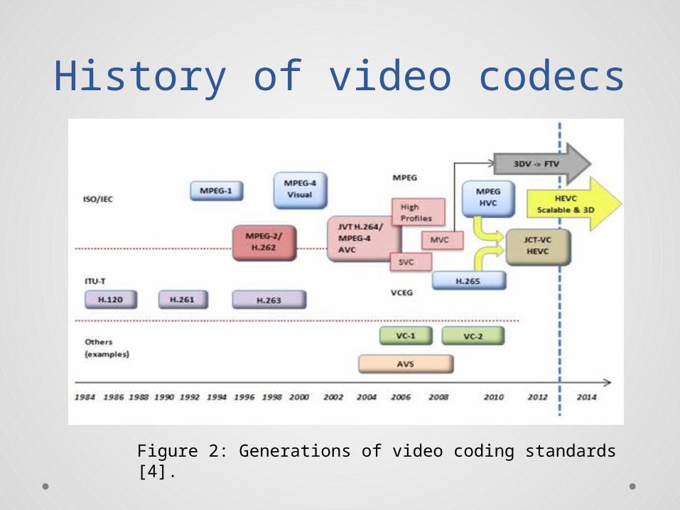
Figure 2: Generations of video coding standards [4].

Introduction to HEVC

Introduction to HEVC

• HEVC standard doubles the coding efficiency and the approximately 50%

less bit rate with respect to H.264/AVC, at approximately the same video

quality. HEVC encoders are relatively more complex than its predecessors

whereas the decoder complexity has only slightly increased which makes

HEVC applicable to already existing hardware with very few amendments

[10], [12].

• The basic design of HEVC remained the same as that of H.264/AVC i.e., the

block based hybrid coding approach which efficiently exploits the temporal

statistical dependencies, spatial statistical dependencies to maximum [7].

Figure 3: HEVC encoder with decoder

elements shaded in gray [7].

Figure 4: HEVC decoder block

diagram [9]

QUAD TREE STRUCTURE• To start with the encoding process one needs to know the quad-tree

in detail.• CTU as it is the root of quad-tree.• CTU is made of a luma coding tree block (CTB), two chroma CTB

and corresponding quad-tree syntax, where the luma CTB is a block of size NxN and chroma CTBs are of size (N/2)x(N/2). N is chosen inside the bit stream and can be 16, 32 or 64.

• The size of CTB is largest supported size of coding block (CB). CTB may contain one or more coding units (CU).

• CU has an associated partitioning into prediction units (PUs) and transform units (TUs).

• The coding mode, intra or inter prediction, is selected at CU level. [7], [11], [12].

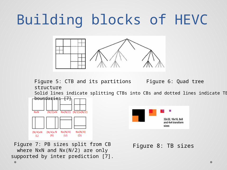
Building blocks of HEVC

Figure 5: CTB and its partitions Figure 6: Quad tree structureSolid lines indicate splitting CTBs into CBs and dotted lines indicate TB boundaries [7]

Figure 7: PB sizes split from CB where NxN and Nx(N/2) are only supported by

inter prediction [7].

Figure 8: TB sizes

Figure 9: Pictorial representations of

various block divisions and

subdivisions

Slices and tiles•  Slices and tiles are used in coding of predicted frames.

o A slice can be defined as a group of CTUs in an independent slice segment and all dependent slice segments. A slice segment can be defined as group of CTUs ordered consequently in a tile scan and contained in a NAL unit.

o A tile can be defined as a rectangular region containing a group of CTUs in a CTB raster scan.

tile boundary

Figure 10: Tile and slice division 1 [12] Figure 11: Tile and slice division 2 [12]

Overview of HEVC intra coding

Overview of HEVC intra coding

The basic elements in the HEVC intra coding design are shown below [15]:1) Quad tree-based coding structure;2) 33 prediction directions for angular predictions;3) Planar prediction to generate smooth sample surfaces;4) Adaptive smoothing of the reference samples;5) Filtering of the prediction block boundary samples;6) Residual transform and coefficient scanning;7) Intra mode coding based on contextual information;

Angular Intra Prediction

0-5-10-15-20-25-30

-30

-25

-20

-15

-10

-5

0

5 10 15 20 25 30

5

10

15

20

25

30

Figure12: 33 Intra prediction directions [12].

Table 1: PU sizes and corresponding

number of intra prediction[7]

Pediction size Number of intra

prediction

64x64 4

32x32 35

16x16 35

8x8 35

4x4 18

Figure 14: Intra prediction angular

orientation and example of direction mode

29 [7].

Table 2: Mapping between intra prediction

direction and intra prediction mode for chroma

[11].

Chroma Intra prediction

mode

Intra prediction direction

0 26 10 1 X ( 0 <= X < 35

 )

0 34 0 0 0 0

1 26 34 26 26 26

2 10 10 34 10 10

3 1 1 1 34 1

4 0 26 10 1 X

Rate Distortion Optimization (RDO)

• With the increase in number of modes and prediction methods in HEVC the complexity also increased, so to decrease the complexity the selection of best mode and prediction me. Mode selection problem is overcome by optimization of the procedure to minimize the distortion (D) for a given bit rate (R) to get the least cost (J).

J = D + λ · R……………………………………. (1)• The RDO selection algorithm attempts to derive best combination that

minimizes the cost. So there is trade-off between Rate and Distortion which can be controlled by the Lagrange multiplier λ. A smaller λ will minimize D, with the effect of increased R whereas a larger λ will minimize R at the expense of a higher D. Selecting the best λ for a particular cost equation is the task of the algorithm described in this thesis

Comparison between HEVC and H.264/AVC

Comparison between HEVC and H.264/AVC

HEVC provides better compression at increased processing power or the coding efficiency is improved significantly for high resolution videos but encoder complexity is much higher than H.264. With the introduction of HEVC into market almost all appliances, applications and software systems will start using HEVC as this gives almost twice the. The major achievements of HEVC in comparison with H.264 are [8]:• Flexible prediction modes and transform block sizes and better partitioning

options.• Improved interpolation and deblocking filters, prediction and signaling of

modes and motion vectors.• Support efficient parallel processing.

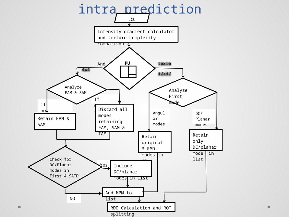
Proposed fast intra prediction

NO

Figure 15: Fast algorithm for intra

prediction

PU size

 

 

 

 

 

 

 

 

 

 

 

 

 

 

Intensity gradient calculator and texture complexity comparison

 

And 16x16

32x32

4x4

8x8

Analyze Firstmode

If neighbors

If not neighbors

Retain FAM & SAM

Discard all modes retaining FAM, SAM & TAM

Retain original 3 RMD modes in list

Retain only DC/planar mode in list

Analyze FAM & SAM

Add MPM to list

Angular modes

DC/Planarmodes

RDO Calculation and RQT splitting

Yes

Include DC/planar modes in list

Check for DC/Planar modes in First 4 SATD

LCU

Step by step process of the proposed

technique

The fast algorithm used in this thesis is explained in an elaborate step by step process:

Step 1: In HEVC, a picture is divided into a sequence of LCUs (large CUs) and further into CUs. The LCU is divided into the smallest (4x4) unit and the intensity gradient calculator is applied to extract the texture complexity and the texture direction of the LCU. Fine CU partition is used for textured region and coarse CU partition is to be used for homogenous region. Then go to step 2.

Step 2: Texture gradient calculations: Intensity gradient of pixel at (x, y) coordinates, g(x, y), is derived from sample of image to be predicted p(x, y).The intensity gradients are calculated for all four possible directions to explore the texture complexity of the original LCU [19].

(a) Horizontal gradient: The intensity gradient formulae for horizontal orientation are as follows [19]:

gh(x, y) = |p(x, y) − p(x + 2, y)| ……………………………….(1a)

gh(x + 1, y) = |p(x + 1, y) − p(x + 3, y)| ………………………..(1b)

gh(x, y + 1) = |p(x, y + 2) − p(x + 2, y + 2)| ……………………(1c)

gh(x + 1, y + 1) = |p(x + 1, y + 2) − p(x + 3, y + 2)| ……………(1d)

Step by step process of the proposed

technique(b) Vertical gradient: The intensity gradient formulae for vertical orientation are as follows [19]:

gv(x; y) = |p(x; y) − p(x + 2; y)| ………………………. …(2a)

gv(x + 1; y) = |p(x + 1; y) − p(x + 3; y)| …………………(2b)

gv(x; y + 1) = |p(x; y + 2) − p(x + 2; y + 2)| ……………. (2c)

gv(x + 1; y + 1) = |p(x + 1; y + 2) − p(x + 3; y + 2)| ……. (2d)

(c) Left-down gradient: The intensity gradient formulae for left-down orientation are as follows [19]:

gld(x, y) = |p(x, y) − p(x + 2, y)| …………………................ (3a)

gld(x + 1, y) = |p(x + 1, y) − p(x + 3, y)| ………………….... (3b)

gld(x, y + 1) = |p(x, y + 2) − p(x + 2, y + 2)| ………………... (3c)

gld(x + 1, y + 1) = |p(x + 1, y + 2) − p(x + 3, y + 2)| ……….. (3d)

(d) Right-down gradient: The intensity gradient formulae for right-down orientation are as follows [19]:

grd(x, y) = |p(x, y) − p(x + 2, y)| …………………….…………. (4a)

grd(x + 1, y) = |p(x + 1, y) − p(x + 3, y)| ……………………….. (4b)

grd(x, y + 1) = |p(x, y + 2) − p(x + 2, y + 2)| …………................ (4c)

grd(x + 1, y + 1) = |p(x + 1, y + 2) − p(x + 3, y + 2)| …………... (4d)

Step by step process of the proposed technique

(x, y)

(x+1,

y)

(x+2,

y)

(x+3,

y)

(x,

y+1)

(x+1,

y+1)

(x+2,

y+1)

(x+3,

y+1)

(x,

y+2)

(x+1,

y+2)

(x+2,

y+2)

(x+3,

y+2)

(x,

y+3)

(x+1,

y+3)

(x+2,

y+3)

(x+3,

y+3)

The gradient is angular if it is almost equal or equal to zero [18]. The intensity gradient is applied in four directions namely horizontal, vertical, right-down and left-down as shown in figure 16 a and the pixels positions of a 4x4 block are shown in figure 16 b:

16 a: Directions of the intensity gradients.

16 b: The positions of the pixels considered in the gradient calculation in a 4x4 LCU.

All four directional gradients are derived by using above equations for each 4x4 LCU. After that sum of absolute gradient for any PU size at all four directions is calculated using the equation 4.5 [19]:

SAG = Σ | g (x, y) | ………………….(5)

To determine the actual texture complexity, normal direction gradient is introduced which determines the actual texture strength. SAG of texture orientation is SAGmin and that of the orthogonal orientation is SAGort, and complexity is calculated as a difference of these values and a threshold (T), where T is QP times PU size (PUsize) as shown in equations 1 and 4 [19]:

Complexity = SAGort - SAGmin ………………… (6)

T = QP x PUsize …………………………………..(7)

If complexity is less than threshold then PU is homogeneous. If CU has more PUs and they are also homogeneous then they are merged together. A CU is thus divided into number of PUs based on equations (1) thru (7) (fig 17). [19]

Step by step process of the proposed

technique

Figure 17: CU division into PUs based on

homogeneousness of the image

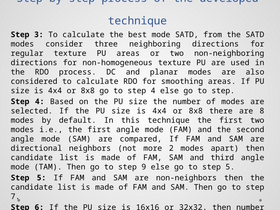
Step 3: To calculate the best mode SATD, from the SATD modes consider three neighboring directions for regular texture PU areas or two non-neighboring directions for non-homogeneous texture PU are used in the RDO process. DC and planar modes are also considered to calculate RDO for smoothing areas. If PU size is 4x4 or 8x8 go to step 4 else go to step.

Step 4: Based on the PU size the number of modes are selected. If the PU size is 4x4 or 8x8 there are 8 modes by default. In this technique the first two modes i.e., the first angle mode (FAM) and the second angle mode (SAM) are compared, If FAM and SAM are directional neighbors (not more 2 modes apart) then candidate list is made of FAM, SAM and third angle mode (TAM). Then go to step 9 else go to step 5.

Step 5: If FAM and SAM are non-neighbors then the candidate list is made of FAM and SAM. Then go to step 7.

Step 6: If the PU size is 16x16 or 32x32, then number of modes by default are only 3 and all the modes are taken into list if no DC or planar mode then go to 7 else go to step 8.

Step by step process of the developed

technique

Step by step process of the developed

technique

Step 7: Check if DC or planar mode exists in first ‘l’ SATD medium modes ( l is 4 in case of 4x4/8x8 and 3 for others), if yes then add them to candidate list but if the PU is 4x4 or 8x8 PU go to step 9 else go to step 8.

Step 8: Add the MPM to the list.

Step9: With this reduced number of PU sizes and prediction modes the total cost is calculated.

To increase the efficiency and reduce the complexity, the process of RQT splitting is simplified in addition to optimized fast intra coding. The RQT depth maximum is set to one in this technique. The block diagram of the fast intra prediction is shown in the figure 4.3.

Experimental results

Experimental resultsTable 3: The encoding time gain, loss in PSNR and bit rate increase of

the proposed fast intra coding HEVC with original HEVC

Test sequence

Size ClassΔ TEnc

Time gain %

Bit Rate% increase

PSNR (dB) loss

Traffic2560x1

600Class

A51 -0.78 -0.072

Parkscene1920x1

080Class

B52 -0.67 -0.098

RaceHorses

832x480

Class C

39 -1.78 -0.085

BQSquare416x24

0Class

D47 -2.26 -0.12

Average Gain

47.25 -1.37 -0.09375

Figure 18: Encoding time gain

Traffic Parkscene RaceHorses BQSquare0

10

20

30

40

50

60

Encoding time improvement of proposed fast intra coding codec wrt HEVC HM 9

Test sequences

Encodin

g t

ime i

mpro

vem

ent

(%)

Table 4: PSNR and bit rate values for proposed HEVC,

original HEVC and H.264 for Traffic test sequence.

QP

Proposed

HEVC-Bit rate (kbps)

Proposed HEVC-

PSNR(dB)

Original HEVC

- Bit rate

(kbps)

Original HEVC -

PSNR(dB)

H.264 - Bit rate

(kbps)

H.264 - PSNR(dB)

40 36.87 37.73 36.59 37.80 53.79 37.40

30 61.79 38.92 61.29 39.00 91.93 38.50

24 79.80 39.94 79.28 40.00 121.30 39.00

20 136.59 42.03 135.36 42.11 197.63 41.90

Figure 19: Bit rate (kbps) vs. PSNR (dB) of proposed HEVC,

original HEVC and H.264 for Traffic test sequence.

 

20.00 40.00 60.00 80.00 100.00 120.00 140.00 160.00 180.00 200.00 220.0035.00

36.00

37.00

38.00

39.00

40.00

41.00

42.00

43.00

Traffic - 30 frames - Class A

proposed HEVCoriginal HEVCH.264

Bit rate ( kbps )

PSN

R(d

B)

Table 5: PSNR and bit rate values for proposed HEVC,

original HEVC and H.264 for Parkscene test sequence

QP

Proposed

HEVC-Bit rate (kbps)

Proposed HEVC-

PSNR(dB)

Original HEVC

- Bit rate

(kbps)

Original HEVC -

PSNR(dB)

H.264 - Bit rate

(kbps)

H.264 - PSNR(dB)

40 24.47 38.47 24.30 38.57 35.72 38.10

30 54.90 39.90 54.57 40.00 81.85 39.00

24 73.31 41.42 72.87 41.50 111.49 41.10

20 120.53 44.99 119.56 45.10 174.56 44.70

Figure 20: Bit rate (kbps) vs. PSNR (dB) of proposed HEVC, original

HEVC and H.264 for test sequence Parkscene

0.00 20.00 40.00 60.00 80.00 100.00 120.00 140.00 160.00 180.00 200.0037.00

38.00

39.00

40.00

41.00

42.00

43.00

44.00

45.00

46.00

Parkscene - 30 frames - Class B

Proposed HEVCOriginal HEVCH.264

Bit rate (kbps)

PSN

R(d

B)

Table 6: PSNR and bit rate values for proposed HEVC,

original HEVC and H.264 for Racehorses test sequence

QP

Proposed

HEVC-Bit rate (kbps)

Proposed HEVC-

PSNR(dB)

Original HEVC - Bit rate (kbps)

Original HEVC -

PSNR(dB)

H.264 - Bit rate

(kbps)

H.264 - PSNR(dB)

40 22.63 36.50 22.18 36.59 32.61 34.00

30 35.11 37.71 34.56 37.80 51.84 34.70

24 63.36 39.82 62.23 39.90 95.21 36.00

20 101.90 43.02 100.11 43.10 146.15 42.90

Figure 21: Bit rate (kbps) vs. PSNR (dB) of proposed HEVC,

original HEVC and H.264 for test sequence Racehorses.

0.00 20.00 40.00 60.00 80.00 100.00 120.00 140.00 160.0033.00

35.00

37.00

39.00

41.00

43.00

Racehorses - 30 frames - Class C

Proposed HEVCOriginal HEVCH.264

Bit rate (kbps)

PSN

R(d

B)

Table 7: PSNR and bit rate values for proposed HEVC,

original HEVC and H.264 for BQ Square test sequence

QP

Proposed

HEVC-Bit rate (kbps)

Proposed HEVC-

PSNR(dB)

Original HEVC

- Bit rate

(kbps)

Original HEVC -

PSNR(dB)

H.264 - Bit

rate (kbps

)

H.264 - PSNR(dB)

40 5.29 34.57 5.17 34.67 7.93 34.20

30 7.47 37.05 7.28 37.23 11.13 37.00

24 10.09 40.01 9.88 40.10 13.11 39.20

20 13.19 43.40 12.95 43.50 18.47 42.90

Figure 22: Bit rate (kbps) vs. PSNR (dB) for proposed HEVC,

HEVC and original H.264 for test sequence BQ Squares.

4.00 6.00 8.00 10.00 12.00 14.00 16.00 18.00 20.0033.00

35.00

37.00

39.00

41.00

43.00

45.00

BQ Square - 30 frames - Class D

Proposed HEVCOriginal HEVCH.264

Bit rate (kbps)

PSN

R(d

B)

Figure 23: QP vs BD-bit rate (kbps) between proposed HEVC

and original HEVC for test sequence Traffic.

20 24 30 409.5

10

10.5

11

11.5

12

12.5

13

BD-bit rate gain - Traffic- Class A

QP

BD

-bit

rate

(kbps)

Figure 24: QP vs BD-bit rate (kbps) between proposed HEVC

and original HEVC for test sequence Parkscene.

20 24 30 4012.5

13

13.5

14

14.5

15

15.5

16

16.5

17

BD-bit rate gain - Parkscene - Class B

QP

BD

-bit

rate

(kbps)

Figure 25: QP vs BD-bit rate (kbps) between proposed HEVC

and original HEVC for test sequence RaceHorses.

20 24 30 4012

12.5

13

13.5

14

14.5

15

15.5

BD-bit rate gain - RaceHorses -- Class C

QP

BD

-bit

rate

(kbps)

Figure 26: QP vs BD-bit rate (kbps) between proposed HEVC

and original HEVC for test sequence BQSquare

20 24 30 4012.4

12.6

12.8

13

13.2

13.4

13.6

13.8

14

14.2

14.4

BD-bit rate gain - BQSquare - Class D

QP

BD

-bit

rate

(kbps)

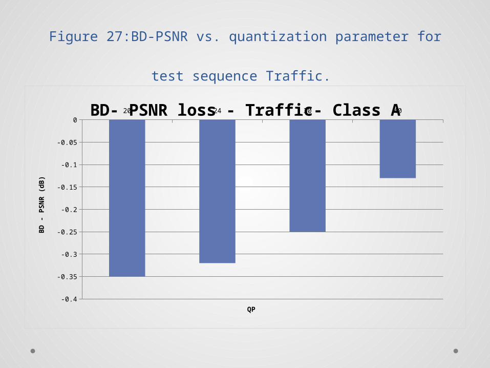
Figure 27:BD-PSNR vs. quantization parameter for test

sequence Traffic.

20 24 30 40

-0.4

-0.35

-0.3

-0.25

-0.2

-0.15

-0.1

-0.05

0BD- PSNR loss - Traffic- Class A

QP

BD

- P

SN

R (

dB

)

Figure 28:: BD-PSNR vs. quantization parameter for test

sequence Parkscene.

20 24 30 40

-0.6

-0.5

-0.4

-0.3

-0.2

-0.1

0

BD- PSNR loss- Parkscene- Class B

QP

BD

-PSN

R (

dB

)

Figure 29:BD-PSNR vs. quantization parameter for test

sequence Racehorses.

20 24 30 40

-0.5

-0.45

-0.4

-0.35

-0.3

-0.25

-0.2

-0.15

-0.1

-0.05

0

QP

BD

- P

SN

R (

dB

)

Figure 30: BD-PSNR vs. quantization parameter for test sequence BQ Square

20 24 30 40

-0.45

-0.4

-0.35

-0.3

-0.25

-0.2

-0.15

-0.1

-0.05

0

BD-PSNR loss - BQSquare - Class D

QP

BD

- P

SN

R (

dB

)

Conclusion

Conclusion• The proposed technique reduced the encoding

time alone at the cost of slight increase in bit rate and negligible PSNR loss. There is an average gain of 47.25% encoder time at very less loss in performance with high complexity reduction.

• The average increase in bit rate is only 1.37 % and average loss in PSNR is only 0.93 dB. In comparison with H.264 [1] standard the average encoding time is larger by only 10%.

Hence this research obtains half the bit rate at almost the same complexity as that of H.264 at almost the same quality.

Applications• The proposed technique reduces the encoding time

significantly. The encoding time at the transmitter end is very critical in practical system and operations like scaling (mobile applications), video uploading and updating storage systems which require movement of large video files etc.. This will in turn reduce over-all time consumed in processing the videos saving many man hours.

• In transmission and general consumer applications like TVs, internet video, and educational websites with video lectures etc., the critical aspect is the speed of download or upload. This greatly reduces the encoding time which reduces the time required to compress the raw videos.

Future Work

Future Work• The complexity reduction in the proposed technique optimizes intra coding of HEVC,

resulting in complexity reduction - inter coding of HEVC can also be optimized. The presented technique can be combined with other fast intra/inter prediction techniques to achieve better bit rate and to improve PSNR.

• Wang et al [36] present a technique which studies multiple sign bit hiding scheme in HEVC. This technique designs quantization of transform coefficients coding by data hiding approach achieving good RDO resulting in overall coding gain in HEVC. This method if combined with the proposed thesis can give very good optimization.

• Vasudevan [31] has adopted a fast intra coding technique in combination with a fast RQT optimization method. This method can be applied with the proposed technique to further reduce the encoder complexity.

Future research can be conducted to improve both the intra and inter coding to obtain much higher reduction of encoding time, better bit rate and PSNR. The aim should be to reduce the overall complexity of HEVC encoder suitable for hand held devices as well as transmission with limited computing resources.

References

References[1] K. Sayood, “Introduction to Data Compression", 4th ed. Morgan Kaufmann, 2012.

[2] Y.Q. Shi , and H. Sun, “Image and video compression for multimedia engineering: fundamentals, algorithms, and standards”, Boca Raton, Fla: CRC Press, 1999.

[3] I. Richardson, “The H.264 Advanced Video Compression Standard", Wiley, 2010.

[4] N. Ling, “High efficiency video coding and its 3D extension: A research perspective," 7th IEEE, Trans. on ICIEA, pp. 2150-2155, July 2012.

[5] K.R. Rao, D.N. Kim and J.J. Hwang, “Video coding standards: AVS China, H.264/MPEG4-Part 10, HEVC, VP6, DIRAC and VC-1”, Springer 2014.

[6] J. Chen, U. Koc, and K. Liu, “Design of Digital Video Coding Systems A Complete Compressed Domain Approach", Marcel Dekker, 2002.

[7] G.J. Sullivan; J. Ohm; W.-J. Han and T. Wiegand, “Overview of the High Efficiency Video Coding (HEVC) Standard”, IEEE Trans. on CSVT, vol. 22, Issue: 12, pp. 1649-1668, Dec 2012.

[8] F. Bossen, D. Flynn and K. Suhring, “HEVC reference software manual”, July 2011. [Online]. Available:

http://phenix.int-evry.fr/jct/doc_end_user/documents/6_Torino/wg11/JCTVC-F634-v2.zip

[9] B. Bross et al, “High efficiency video coding (HEVC) text specification draft 10”, 12th Meeting Geneva January 2013. [Online]. Available:

http://phenix.it-sudparis.eu/jct/doc_end_user/current_document.php?id=7243

[10]F. Bossen, B. Bross, K. Sühring, and D. Flynn, "HEVC Complexity and Implementation Analysis," IEEE Trans. on CSVT, vol.22, no.12, pp.1685-1696, Dec. 2012.

References [11] B. Bross et al, “HM9: High Efficiency Video Coding (HEVC) Test Model 9 Encoder Description”, JCTVC-K1002v2, October 2012. [Online]. Available:

http://phenix.it-sudparis.eu/jct/doc_end_user/current_document.php?id=6807

[12] B. Bross et al, “High Efficiency Video Coding (HEVC) text specification draft 9 (SoDIS)”, JCTVC-K1003v13, October 2012. [Online]. Available:

http://phenix.it-sudparis.eu/jct/doc_end_user/current_document.php?id=6803

[13] J.-R. Ohm et al, “Comparison of the coding efficiency of video coding standards – including high efficiency video coding (HEVC)”, IEEE Trans. on CSVT, vol. 22, pp.1669-1684, Dec. 2012.

[14] I. Richardson., “HEVC: An introduction to High Efficiency Video Coding”, [Online]. Available: https://www.vcodex.com/images/uploaded/452853087451536.pdf

[15] J. Lainema et al, “Intra coding of the HEVC standard”, IEEE Trans. on CSVT, vol. 22, pp. 1792-1801, Dec. 2012.

[16] Y. Zhang, C. Zhao and J. Xu, “An adaptive fast intra mode decision in HEVC”, IEEE ICIP 2012, pp. 221-224, Orlando, FL, Sept.-Oct., 2012.

[17] Y. Zhang, Z. Li and B. Li, “Gradient-based fast decision for intra prediction in HEVC”, IEEE VCIP 2012, pp. 1-6, Nov. 2012.

[18] A-C Tsai, A. Pal, J. Ching Wang, and J-F Wang, “Intensity gradient technique for efficient intra-prediction in h.264/AVC,” IEEE Trans. on CSVT, vol. 18, no. 5, pp. 694–698, May. 2008.

References[19] W. Y. Ma and B. S. Manjunath, “A texture thesaurus for browsing large aerial photographs,” J. Amer. Soc. Inf. Sci.,vol. 49, no. 7, pp. 633–648, May. 1998.

[20] L.-L. Wang and W.-C. Siu.“Novel adaptive algorithm for intra prediction with compromised modes skipping and signaling processes in HEVC”, IEEE Trans. on CSVT, vol. 23, pp. 1686-1694, Nov. 2013.

[21] D. Flynn, J. Sole, T. Suzuki (2013-08-07). "High Efficiency Video Coding (HEVC) Range Extensions text specification: Draft 4". JCT-VC.Retrieved 2013-08-07. [22] “HM reference software svn repository." [Online]. Available:

http://hevc.hhi.fraunhofer.de/svn/svn_HEVCSoftware/

[23] JM11 reference software JM11KTA2.3 [Online]. Available:

http://www.h265.net/2009/04/kta-software-jm11kta23.html

[24] G. Correa et al, “Performance and computational complexity assessment of high efficiency video encoders”, IEEE Trans. on CSVT, vol. 22, pp.1899-1909, Dec. 2012.

[25] G. Bjontegaard, “Calculation of average PSNR differences between RD-Curves”, ITU-T SG16, Doc. VCEG-M33, 13th VCEG meeting, Austin, TX, April 2001. [Online]. Available:

http://wfpt3.itu.int/av-arch/video-site/0104_Aus/VCEG-M33.doc

[26] Open source article, “Bit rate”. [Online]. Available: http://en.wikipedia.org/wiki/Bit_rate

[27] Open source article on “video resolution”. [Online]. Available: http://www.newfangled.com/designing_for_changing_web_content_and_context

[28] Repository for freely-redistributable test sequences.[Online] Available: www.media.xiph.org.

[29] “Test video sequences." [Online]. Available:

ftp://hvc:US88Hula@ftp.tnt.uni-hannover.de/testsequences

[30] Open source website “Practical guide to CCTV video resolutions. [Online]. Available: http://optiviewusa.com/cctv-video-resolutions.aspx

[31] S. Vasudevan,“Implementation of fast residual quadtree coding and fast intra prediction in high efficiency video coding”, EE Dept., University of Texas at Arlington, UMI dissertation publishing, Dec. 2013.

[32] Special issue on video coding: HEVC and beyond, IEEE journal of selected topics in signal processing, Dec. 2013.

[33] G. Bjontegaard, “Calculation of average PSNR differences between RD-curves”, Q6/SG16, Video Coding Experts Group (VCEG) ITU-T Standardization Sector, 2-4 April. 2001

[34] BD metrics open source code. [Online]. Available:

http://www.mathworks.com/matlabcentral/fileexchange/27798bjontegaardmetric/content/bjontegaard.m

[35] Open source article on “PSNR”. [Online]. Available:

http://en.wikipedia.org/wiki/Peak_signal-to-noise_ratio#cite_note-8

[36] J. Wang et al, “Multiple sign bits hiding for high efficiency video coding”, Visual Communications and Image Processing, VCIP 2012, San Diego, CA, 27-30, Nov. 2012.

References