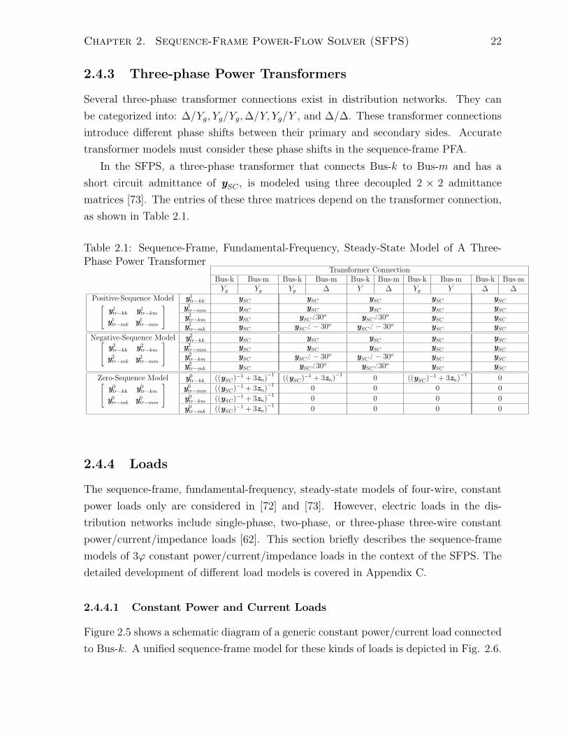
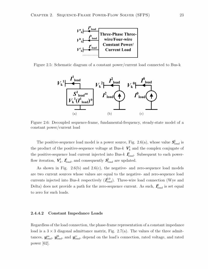
In this thesis, italic symbols indicated phasor quantities, e.g., I, while multi-dimensional
matrices are shown in bold uppercase, e.g., I.
xix
Chapter 1
Introduction
1.1 Active Distribution Networks
1.1.1 Definitions
Driven by technical advancement, political readiness, social awareness, and economical
incentives, the anticipated proliferation of distributed energy resources (DER) units, in-
cluding distributed generation (DG), distributed storage (DS), and controllable loads,
into the current distribution grids close to the load sites, is emerging as a complementary
infrastructure to the traditional central power plants [1,2]. Unless optimally coordinated
and efficiently integrated, the high-depth of DER penetration will bring many technical
challenges in terms of planning and operation of the distribution networks including,
among others, protection mal-coordination, voltage level violations, power quality con-
cerns, and increasing line losses. The need for efficient and safe DER integration schemes
brings about the concept of the “active distribution systems”.
The active distribution system (ADS), also known as active distribution network
(ADN), is the new generation of today’s distribution networks where the DER units are
optimally operated and efficiently integrated. The CIGRE C6.11 working group defines
the ADN as a distribution network whose operator can remotely and automatically con-
trol the DER units and network topology to efficiently manage and optimally utilize the
network assets [3]. In the ADN, the power flow between busses is bidirectional, and
variables are measured (or estimated) and controlled based on a centralized and intelli-
gent system. The central control system is capable of making decisions and operating
the ADN based on monitoring the network conditions. In general, the ultimate goal of
the ADN is to (i) enhance the DER observability and controllability, (ii) deliver cost
efficient integration of the DER units into the distribution network, and (iii) maximize
1
Chapter 1. Introduction 2
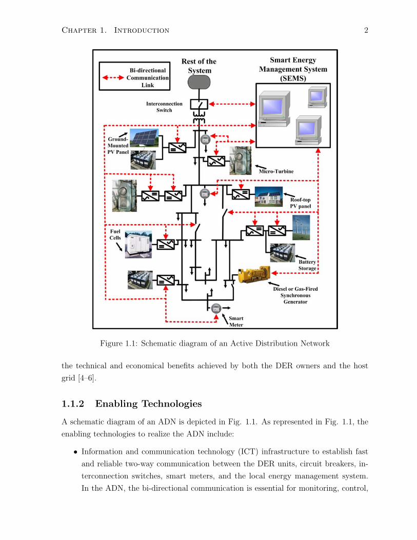
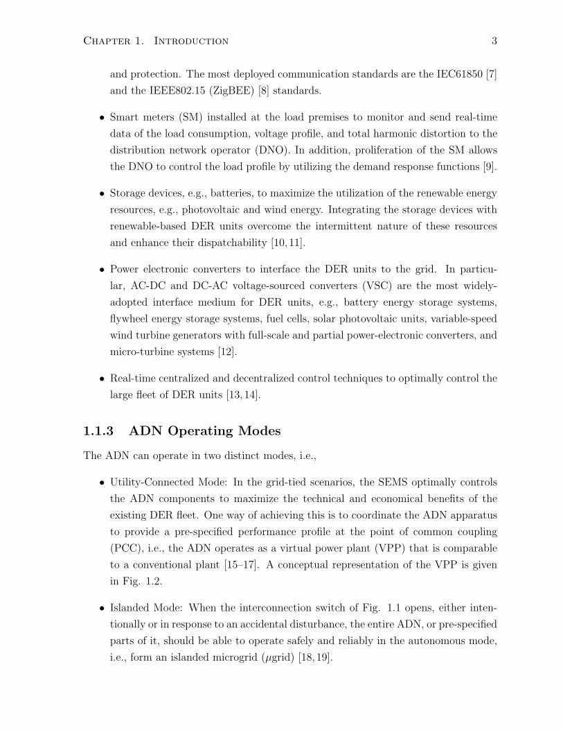
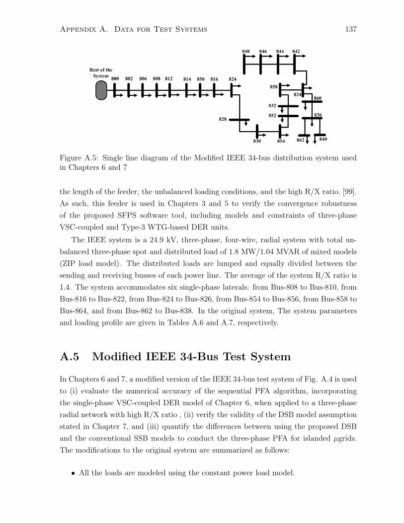
Figure 1.1: Schematic diagram of an Active Distribution Network
the technical and economical benefits achieved by both the DER owners and the host
grid [4–6].
1.1.2 Enabling Technologies
A schematic diagram of an ADN is depicted in Fig. 1.1. As represented in Fig. 1.1, the
enabling technologies to realize the ADN include:
• Information and communication technology (ICT) infrastructure to establish fast
and reliable two-way communication between the DER units, circuit breakers, in-
terconnection switches, smart meters, and the local energy management system.
In the ADN, the bi-directional communication is essential for monitoring, control,
Chapter 1. Introduction 3
and protection. The most deployed communication standards are the IEC61850 [7]
and the IEEE802.15 (ZigBEE) [8] standards.
• Smart meters (SM) installed at the load premises to monitor and send real-time
data of the load consumption, voltage profile, and total harmonic distortion to the
distribution network operator (DNO). In addition, proliferation of the SM allows
the DNO to control the load profile by utilizing the demand response functions [9].
• Storage devices, e.g., batteries, to maximize the utilization of the renewable energy
resources, e.g., photovoltaic and wind energy. Integrating the storage devices with
renewable-based DER units overcome the intermittent nature of these resources
and enhance their dispatchability [10,11].
• Power electronic converters to interface the DER units to the grid. In particu-
lar, AC-DC and DC-AC voltage-sourced converters (VSC) are the most widely-
adopted interface medium for DER units, e.g., battery energy storage systems,
flywheel energy storage systems, fuel cells, solar photovoltaic units, variable-speed
wind turbine generators with full-scale and partial power-electronic converters, and
micro-turbine systems [12].
• Real-time centralized and decentralized control techniques to optimally control the
large fleet of DER units [13,14].
1.1.3 ADN Operating Modes
The ADN can operate in two distinct modes, i.e.,
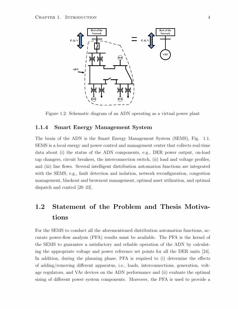
• Utility-Connected Mode: In the grid-tied scenarios, the SEMS optimally controls
the ADN components to maximize the technical and economical benefits of the
existing DER fleet. One way of achieving this is to coordinate the ADN apparatus
to provide a pre-specified performance profile at the point of common coupling
(PCC), i.e., the ADN operates as a virtual power plant (VPP) that is comparable
to a conventional plant [15–17]. A conceptual representation of the VPP is given
in Fig. 1.2.
• Islanded Mode: When the interconnection switch of Fig. 1.1 opens, either inten-
tionally or in response to an accidental disturbance, the entire ADN, or pre-specified
parts of it, should be able to operate safely and reliably in the autonomous mode,
i.e., form an islanded microgrid (μgrid) [18, 19].
Chapter 1. Introduction 4
Figure 1.2: Schematic diagram of an ADN operating as a virtual power plant
1.1.4 Smart Energy Management System
The brain of the ADN is the Smart Energy Management System (SEMS), Fig. 1.1.
SEMS is a local energy and power control and management center that collects real-time
data about (i) the status of the ADN components, e.g., DER power output, on-load
tap changers, circuit breakers, the interconnection switch, (ii) load and voltage profiles,
and (iii) line flows. Several intelligent distribution automation functions are integrated
with the SEMS, e.g., fault detection and isolation, network reconfiguration, congestion
management, blackout and brownout management, optimal asset utilization, and optimal
dispatch and control [20–23].
1.2 Statement of the Problem and Thesis Motiva-
tions
For the SEMS to conduct all the aforementioned distribution automation functions, ac-
curate power-flow analysis (PFA) results must be available. The PFA is the kernel of
the SEMS to guarantee a satisfactory and reliable operation of the ADN by calculat-
ing the appropriate voltage and power reference set points for all the DER units [24].
In addition, during the planning phase, PFA is required to (i) determine the effects
of adding/removing different apparatus, i.e., loads, interconnections, generation, volt-
age regulators, and VAr devices on the ADN performance and (ii) evaluate the optimal
sizing of different power system components. Moreover, the PFA is used to provide a
Chapter 1. Introduction 5
precise and efficient initialization approach for eigen analysis, transient stability, and
electro-magnetic transients programs [25,26].
1.2.1 Lack of Tools
The PFA of large power systems is a mature subject and a wide array of production
grade power-flow software tools that represent various power-system components, e.g.,
HVDC converters and FACTS controllers, are widely available [27–29]. However, such
tools are neither tailored for nor adequately address the PFA requirements of the ADN.
The main reasons are:
• the inherent large degree of imbalance of distribution networks due to (i) single-
phase and two-phase loads, (ii) single-phase DER units, (iii) untransposed lines,
and (iv) single-phase laterals [30]. As such, the distribution level PFA should
simultaneously address the three phases,
• the presence of three-phase VSC-based DER units which can include (i) three-wire
configurations, (ii) four-wire configurations, and (iii) various control strategies that
can respond to selected sequence-frame voltage and current components [31–37].
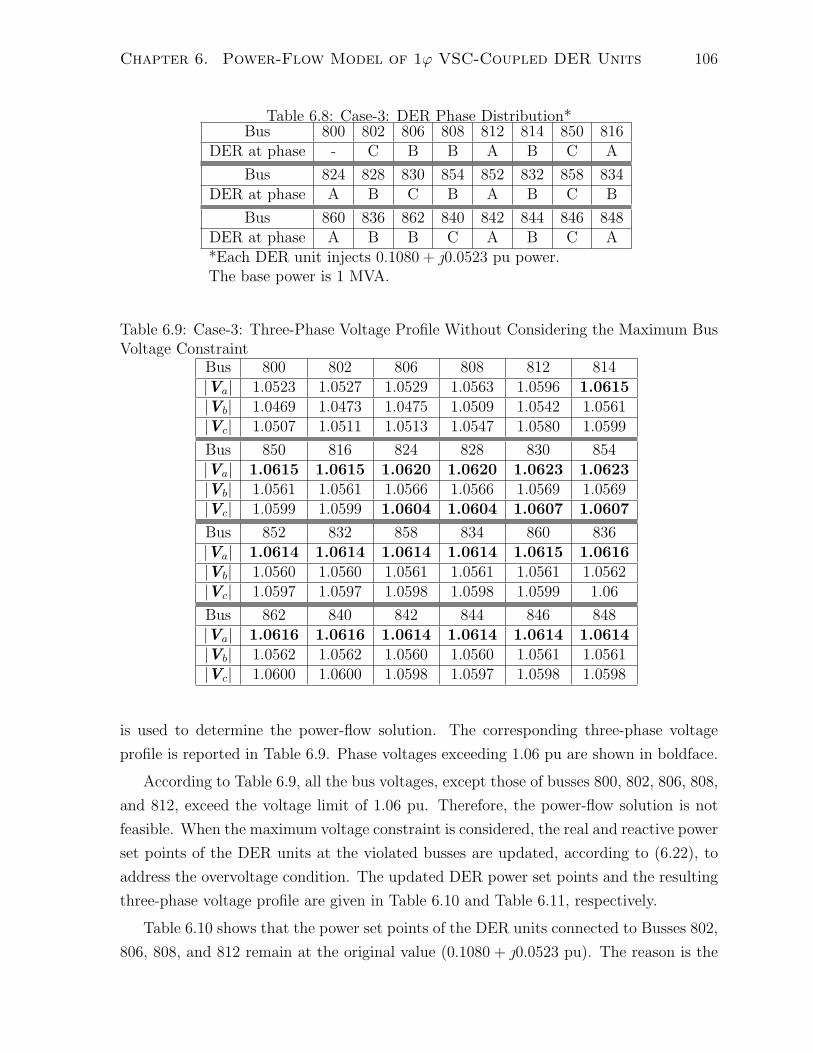
Some production grade software tools provide three-phase power-flow analysis for
distribution networks accommodating DER units [38–40]. However, these tools have the
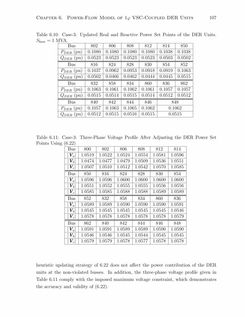
following shortcomings:
• The commercially-available power-flow tools are developed for radial distribution
networks. However, the ADN may be mesh-connected to maximize the DER ben-
efits. Thus, the available tools cannot handle multi-directional power-flow and
general network topologies [34, 41].
• The available three-phase PFA algorithms adopt the phase-frame rather than the
sequence-frame. As will be detailed in Chapter 2, sequence-frame based PFA algo-
rithms are easier to implement, computationally more efficient, and provide flexi-
bility to model VSC-coupled DER units than their phase-frame counterparts.
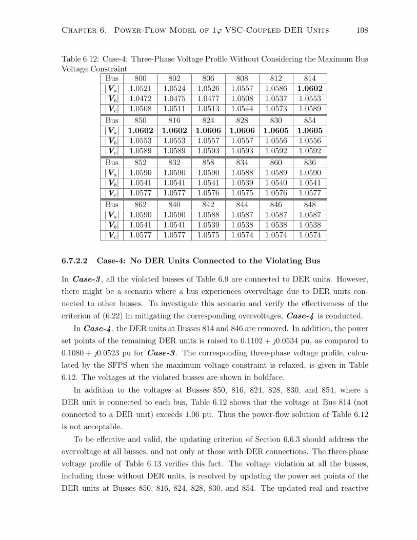
• The available three-phase power-flow engines are not suitable for the islanded μgrid
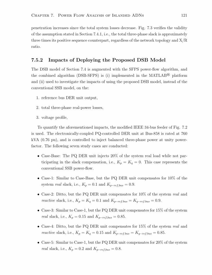
operating mode. The reason is that these tools lack an appropriate three-phase
distributed real- and reactive-slack bus model to conduct the PFA. As will be
discussed in Chapter 7 of this thesis, distributed slack bus (DSB)-based PFA is
vital to conduct the power-flow analysis of the islanded μgrid operating mode since
Chapter 1. Introduction 6
it guarantees that the DER unit connected to the reference bus need not to be an
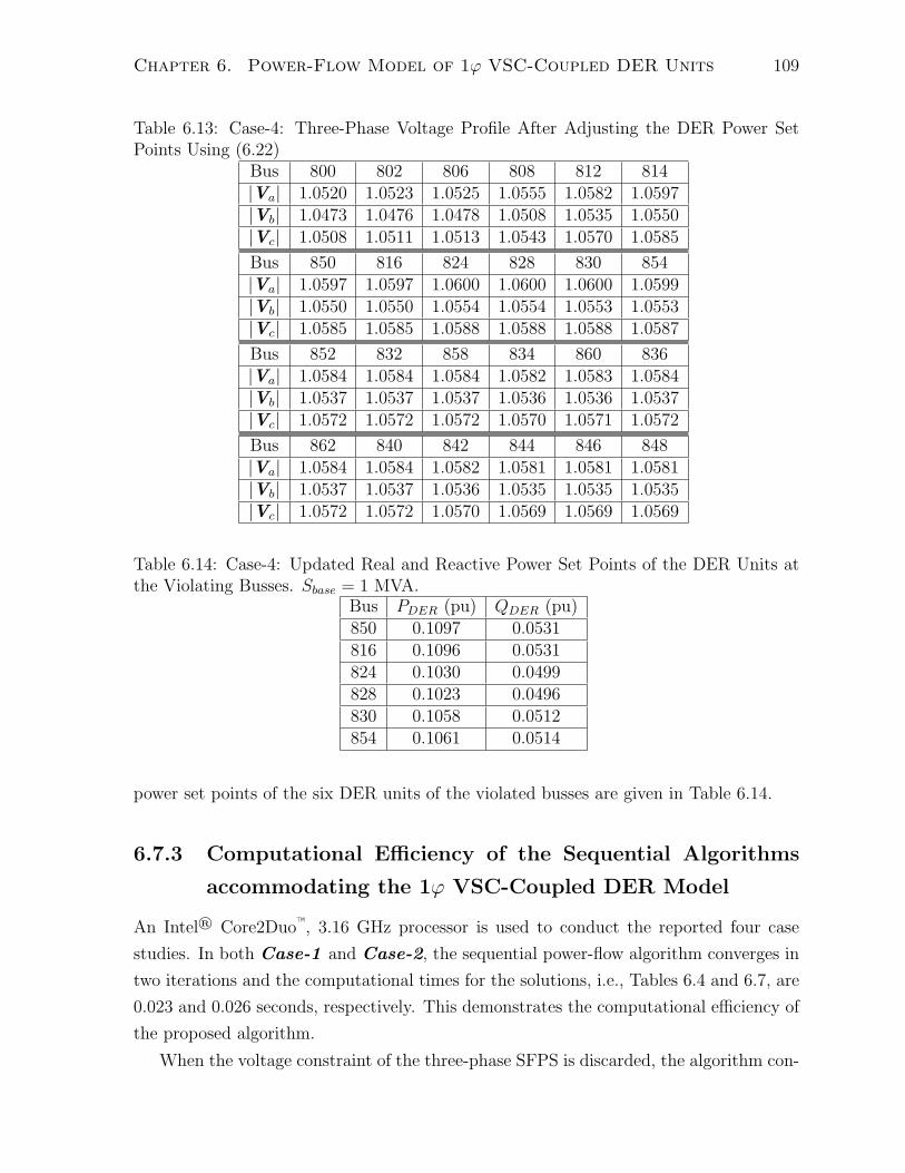
infinite power source [42].
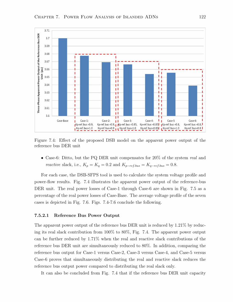
1.2.2 Lack of DER Models
To obtain unerring three-phase PFA results, detailed and accurate three-phase, steady-
state, fundamental-frequency DER models are required. These models should adequately
address (i) different DER types, i.e., rotating machine-based DER units, single-phase
VSC-coupled, three-phase three-wire VSC-coupled, and three-phase four-wire VSC-coupled
DER units, (ii) different control objectives under balanced and unbalanced grid condi-
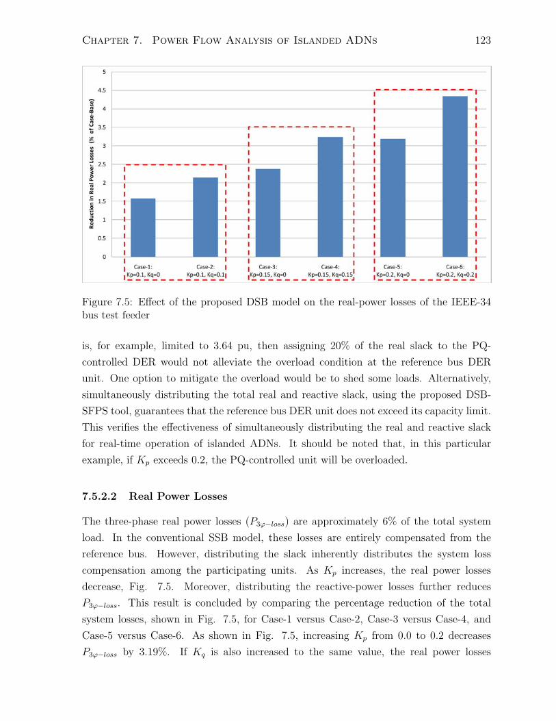
tions, i.e., voltage/frequency and real/reactive-power control, specific control actions to
mitigate the voltage and/or current unbalance at the point of connection, and (iii) the op-
erating limits of the interface VSC and the host DER unit, e.g., the converter modulation
index limit, phase current limit, power capacity limit, and terminal voltage limit.
Modeling of electronic converters for interfacing DER units is one of the most chal-
lenging problems, and is becoming an area of active research relevant to power flow
studies [43]. Developing detailed single- and three-phase VSC-coupled DER models for
the ADN power-flow analysis applications has not been systematically addressed in the
technical literature. The reasons are (i) the current relatively limited proliferation of
the electronically-coupled DER units in the distribution grids and (ii) most of the cur-
rently available DER units are based on constant speed directly-coupled three-phase
synchronous generators. The available electronically-coupled DER models, both in the
technical literature and the production-grade software tools, (i) assume only positive-
sequence DER representation, (ii) do not represent the single-phase VSC-coupled DER
units, (iii) do not address most of the aforementioned control objectives, and (iv) neglect
the interface converter operating limits [31,32,34,44–54].
1.3 Thesis Objectives
Based on the discussion of Section 1.2, the thesis objectives are:
1. Develop detailed and accurate steady-state, fundamental-frequency models of VSC-
based DER units for three-phase PFA. The DER units under study include:
• DER units interfaced via a three-phase front-end three-wire or four-wire VSC,
• Variable-speed wind-turbine-generator (WTG)-based DER units deploying a
Chapter 1. Introduction 7
three-phase doubly-fed asynchronous generator (DFAG), also known as Type-
3 WTG,
• Single-phase VSC-coupled DER units,
The developed DER models should address (i) balanced and unbalanced power-flow
scenarios, (ii) various VSC control strategies under balanced and unbalanced grid
conditions, and (iii) the operating limits and constraints of the VSC and its host
DER unit.
2. Develop a three-phase PFA tool for PFA of analysis and real-time operation of
ADNs. The developed program must:
• be fast and accurate for the real-time management and control of the ADN,
• incorporate the developed single-phase and three-phase DER models, includ-
ing the interface VSC operating constraints in a computationally-efficient man-
ner,
• be capable of analyzing different network topologies (radial, weakly meshed
and meshed networks), including high degrees of unbalance,
• accommodate models of multi-phase power lines and single-phase laterals,
• contain models of single, two, and three-phase loads with different connections,
including constant impedance, current, and power (ZIP) load models,
• accommodate models of three-phase distribution transformers with various
connections, including the phase shift introduced by different transformer con-
nections.
3. Develop a three-phase distributed slack bus (DSB) model. The developed DSB
model will be integrated with the aforementioned tool to conduct three-phase PFA
of islanded ADNs.
1.4 Methodology
1.4.1 Modeling Methodology
The developed DER models and the three-phase PFA tool are developed in the sequence-
components frame. The merits of the sequence-frame compared to the phase-frame for
the three-phase PFA are detailed in Chapter 2 of this thesis.
Chapter 1. Introduction 8
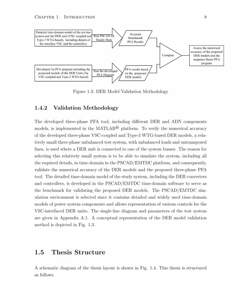
Figure 1.3: DER Model Validation Methodology
1.4.2 Validation Methodology
The developed three-phase PFA tool, including different DER and ADN components
models, is implemented in the MATLAB® platform. To verify the numerical accuracy
of the developed three-phase VSC-coupled and Type-3 WTG-based DER models, a rela-
tively small three-phase unbalanced test system, with unbalanced loads and untransposed
lines, is used where a DER unit is connected to one of the system busses. The reason for
selecting this relatively small system is to be able to simulate the system, including all
the required details, in time-domain in the PSCAD/EMTDC platform, and consequently,
validate the numerical accuracy of the DER models and the proposed three-phase PFA
tool. The detailed time-domain model of the study system, including the DER converters
and controllers, is developed in the PSCAD/EMTDC time-domain software to serve as
the benchmark for validating the proposed DER models. The PSCAD/EMTDC sim-
ulation environment is selected since it contains detailed and widely used time-domain
models of power system components and allows representation of various controls for the
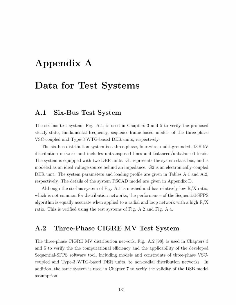
VSC-interfaced DER units. The single-line diagram and parameters of the test system
are given in Appendix A.1. A conceptual representation of the DER model validation
method is depicted in Fig. 1.3.
1.5 Thesis Structure
A schematic diagram of the thesis layout is shown in Fig. 1.4. This thesis is structured
as follows.
Chapter 1. Introduction 9
Figure 1.4: Schematic diagram of the thesis layout
1.5.1 Chapter 2: A Three-Phase Sequence-Frame Power-Flow
Solver (SFPS) Tool
In this chapter, a fast, accurate, and robust three-phase power-flow analysis software
tool is developed for ADN applications, i.e., the SFPS tool. Three-phase, sequence
frame-based, fundamental-frequency, steady-state mathematical models of transformers,
loads, and power-lines are described and accommodated in the SFPS. The SFPS is the
hub into which different types of DER units, including their interfacing media, control
capabilities, and operating limits, are accommodated and tested. This contribution is
detailed in Chapter 2, and published in an IEEE Power Delivery Transactions paper [55]
and a reviewed conference paper [56].
1.5.2 Chapter 3: Steady-State Models of Three-Phase VSC-
Coupled DER Units
In this chapter, a unified sequence frame-based, fundamental-frequency, steady-state
mathematical model of a DER unit interfaced to the grid via a three-phase front-end
VSC is proposed and developed. As detailed in Section 1.1.2, the developed model rep-
resents a wide spectrum of DER types, e.g., battery energy storage systems, fuel cells,
solar photovoltaic units, variable-speed wind turbine generators with full-scale power-
Chapter 1. Introduction 10
electronic converters (Type-4 WTG), and micro-turbine systems. The proposed model is
generic since it accurately addresses (i) three-wire and four-wire VSC configurations, (ii)
balanced and unbalanced power-flow scenarios, (iii) various VSC control strategies, and
(iv) the operating limits and constraints of the interface VSC and the host DER unit.
The developed model is incorporated with the SFPS tool of Chapter 2.
In addition, an enhancement to the basic SFPS algorithm, presented in Chapter 2,
is proposed to model and impose the VSC operating constraints in a computationally-
efficient way. The enhanced algorithm is called the Sequential-SFPS. The computational
efficiency of the Sequential-SFPS is verified by comparing the convergence pattern of
the proposed algorithm against other reported methods. This contribution is detailed in
Chapter 3 and is published in an IEEE Power Delivery Transactions paper [57].
1.5.3 Chapters 4 and 5: Steady-State Models of Type-3 WTG-
Based DER Units
In Chapter 4, I applied the VSC model of Chapter 3 to develop a detailed sequence frame-
based, fundamental-frequency, steady-state mathematical model of a Type-3 WTG-based
DER unit subjected to unbalanced voltage and current conditions. The proposed model
is incorporated with the SFPS, and the Sequential-SFPS of Chapter 3 is extended to
accommodate all the operating limits of the WTG unit and its associated VSCs. A wide
array of case studies are conducted in Chapter 5 to verify the numerical accuracy and
the computational efficiency of the Sequential-SFPS accommodating the proposed Type-
3 WTG-based DER model. A two-part IEEE Sustainable Energy Transactions paper,
describing the details of the proposed DER model and its applications, has been accepted
for publication [58,59].
1.5.4 Chapter 6: Steady-State Models of Single-Phase VSC-
Coupled DER Units
In this chapter, I developed fundamental-frequency, steady-state models of a single-phase
VSC-coupled DER unit for the PFA of single-phase laterals and three-phase distribution
feeders. The proposed models represent different VSC operating modes and constraints.
The sequential approach of Chapter 3 is deployed to impose the VSC constraints into
the power-flow algorithm. The proposed models are integrated with (i) the SFPS for
the PFA of three-phase networks and (ii) a single-phase PFA algorithm to study the
radial single-phase laterals. Several case studies are conducted to evaluate and verify
Chapter 1. Introduction 11
the accuracy of the proposed model. This contribution is detailed in Chapter 6, and an
IEEE Power Delivery Transactions paper, describing the details and applications of the
proposed models, has been submitted and is in review [60].
1.5.5 Chapter 7: Three-Phase Distributed Real- and Reactive-
Slack Bus Model
In this chapter, a novel three-phase sequence frame-based DSB model is described and
augmented with the SFPS of Chapter 2 to conduct three-phase PFA for islanded ADNs.
Unlike the existing DSB models, the proposed formulation (i) simultaneously distributes
the real and reactive power slack and (ii) involves DER units with different control
strategies in slack compensation. A wide array of case studies is conducted to investigate
the impacts of distributing the real and reactive power slack using the three-phase DSB-
SFPS tool. This contribution is detailed in Chapter 7. In addition, an IEEE Smart Grids
Transactions paper [61] is submitted to report this contribution, and is in review.
1.5.6 Chapter 8: Conclusions
The main conclusions of the thesis and the suggestions for future research topics are
listed in Chapter 8.
Chapter 2
Sequence-Frame Power-Flow Solver
(SFPS)1
2.1 Introduction
This chapter lays the foundation of a three-phase power-flow algorithm, in the sequence-
components frame, for ADN applications. The algorithm is called Sequence-Frame
Power-flow Solver (SFPS). Basic ADN components (power-lines, transformers, and loads)
are modeled in the sequence-frame and accommodated in the SFPS to obtain an accu-
rate three-phase steady-state solution. The SFPS is the hub to which models of different
types of electronically-coupled DER units, including their interfacing media, control ca-
pabilities, and operating limits under balanced and unbalanced power-flow scenarios, are
accommodated to construct the integrated 3ϕ power-flow analysis (PFA) tool, as will be
detailed in the next four chapters.
2.2 Three-Phase Power-Flow Analysis: Critical Re-
view
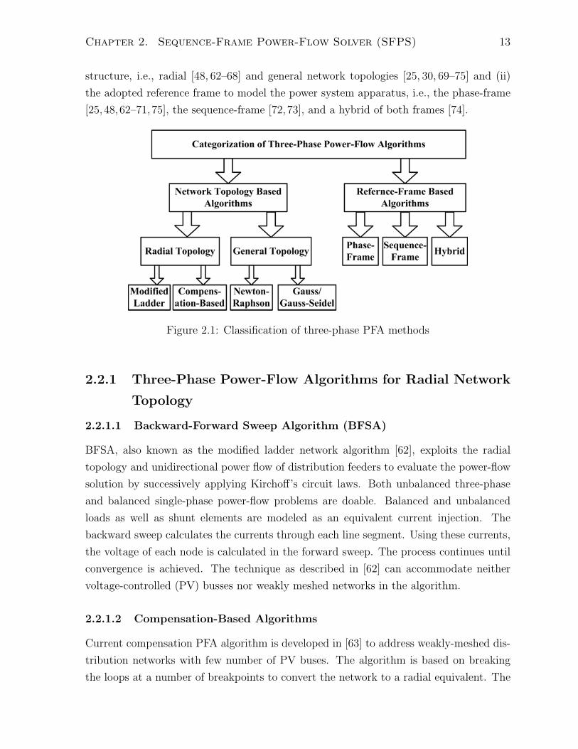
The concept of three-phase PFA has been extensively addressed in the literature. As
shown in Fig. 2.1, the related algorithms are classified according to (i) the network
1The work presented in this chapter has been published and appears in M.Z. Kamh and R. Iravani,“Unbalanced Model and Power-Flow Analysis of Microgrids and Active Distribution Systems,” IEEETrans. Power Delivery, vol.25, no.4, pp.2851-2858, Oct. 2010. An earlier version of this work has beenpresented and appears in M.Z. Kamh and R. Iravani, “Three-Phase Model and Power-Flow Analysisof Microgrids and Virtual Power Plants,” Proc. of the Fourth Canadian CIGRE Conference on PowerSystems, Toronto, Ontario, Canada, October 2009.
positive-sequence real power, P 1DER, both in per-unit, are given by
|V1k| = Vsp, (2.1)
P 1DER =
Psp−DER
3, (2.2)
where Vsp and Psp−DER are the specified per-unit positive-sequence terminal voltage and
the total three-phase injected real power of the TDSG unit respectively.
(a) (b) (c)
Figure 2.2: Sequence-frame, fundamental-frequency, steady-state model of a three-phasedirectly connected synchronous generator for the SFPS: (a) the positive-sequence model,(b) the negative-sequence model, (c) the zero-sequence model
If the TDSG unit operates in the PQ mode, its positive-sequence representation is a
constant power source (or negative constant power load) [85]. The positive-sequence real
power P 1DER is given by (2.2). The positive-sequence reactive power (Q1
DER) injected by
the TDSG unit, in per-unit, is
Q1DER =
Qsp−DER
3, (2.3)
where Qsp−DER is the total three-phase reactive power injected by the TDSG unit. The
factor 1/3 in (2.2) and (2.3) is used to calculate the sequence-frame power components
from their phase-frame counterparts, assuming the same base-power is used in both
reference frames.
The negative- and zero-sequence models of the TDSG unit are shown in Fig. 2.2(b)
and 2.2(c), respectively. The negative- and zero-sequence admittances (y2,0DER) are [86]
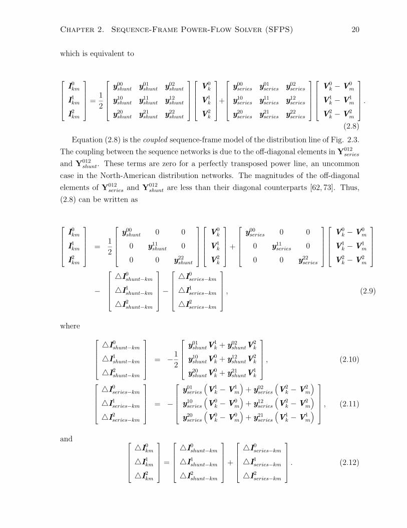
Equation (2.12) represents the equivalent compensation currents that should be in-
jected into Bus-k to decouple the three sequence networks. The equivalent positive-
sequence compensation power (�S1km) injected at Bus-k is given by
�S1km = �P 1
km + j�Q1km = V1
k
(�I1
km
)∗. (2.13)
The decoupled sequence-frame model of the three-phase distribution line is given by (2.9)-
(2.13), and is depicted in Fig 2.4. Implementing the model of Fig. 2.4 in the SFPS is
discussed in Section 2.5
(a)
(b)
(c)
Figure 2.4: Decoupled sequence-frame, fundamental-frequency, steady-state model of athree-phase distribution line: (a) the positive-sequence model, (b) the negative-sequencemodel, (c) the zero-sequence model
The SFPS algorithm, including the details of incorporating the aforementioned com-
ponents, is presented and discussed. The SFPS is the hub into which the VSC-based
DER models are incorporated and tested, as will be detailed in the next four chapters.
Chapter 3
Power-Flow Model of 3ϕ
VSC-Coupled DER Units1
3.1 Introduction
This chapter presents a unified fundamental-frequency, steady-state model of a three-
phase VSC, in the sequence-components frame, for PFA of VSC-interfaced DER units.
The proposed model is unified since it encompasses a wide array of DER units, e.g.,
battery energy storage systems (BESS), fuel cells (FC), solar photovoltaic units (SPV),
variable-speed wind turbine generators with full-scale power-electronic converters (Type-
4 WTG), and micro-turbine (MT) systems. In addition, the model represents (i) three-
wire and four-wire VSC configurations, (ii) balanced and unbalanced power-flow scenar-
ios, (iii) various VSC control strategies, and (iv) operating limits and constraints of the
VSC and its host DER unit. To achieve numerical and computational efficiency, the
SFPS algorithm, presented in Chapter 2, is modified to impose the the interface-VSC
operating limits. The accuracy of the developed model and the computational efficiency
of the modified SFPS are demonstrated based on several case studies. Where applicable,
the numerical accuracy of the VSC model is validated based on comparison with the
exact time-domain solution, using the PSCAD/EMTDC platform.
1The work presented in this chapter has been published and appears in M.Z. Kamh and R. Iravani,“A Unified Three-Phase Power-Flow Analysis Model for Electronically-Coupled Distributed Energy Re-sources,” IEEE Trans. Power Delivery, vol.26, no.2, pp.899-909, April 2011.
32
Chapter 3. Power-Flow Model of 3-ϕ VSC-Coupled DER Units 33
Figure 3.1: Schematic diagram of three-phase VSC-coupled DER unit
3.2 Model Scope and Assumptions
As earlier stated in Chapter 1, three-phase DC-AC VSC is the most widely-adopted
interface medium for DER units [12]. To obtain an accurate power-flow solution of
ADN, three-phase VSC-coupled DER units should be modeled and incorporated in the
SFPS. The proposed model encompasses:
• three-wire and four-wire VSC configurations under both balanced and unbalanced
power-flow scenarios,
• various VSC control strategies, i.e., voltage/frequency and four-quadrant real/reactive
power controls, and specific control actions to inject an/or respond to negative-
and/or zero-sequence components,
• various VSC operational modes, e.g., four-quadrant real-/reactive-power exchange,
• the VSC operational limits and constraints, i.e., maximum phase current, maximum
modulation index, and maximum reactive power limits.
Figure 3.1 shows a schematic diagram of a DER unit coupled to the host system at
Bus-k, which represents the point of connection (PC), via a three-wire or a four-wire
VSC. The primary source is connected to the VSC either (i) directly, e.g., BESS and
FC, (ii) by a DC-DC converter, e.g., SPV, or (iii) by an AC-DC converter, e.g., Type-4
WTG [12,34]. The following assumptions are made:
• The DER primary source is not directly represented in the model as the controllers
of the front-end interface-VSC or the back-end DC-DC converter are assumed to
fully regulate the DC-link voltage under steady-state conditions.
Chapter 3. Power-Flow Model of 3-ϕ VSC-Coupled DER Units 34
(a) (b) (c)
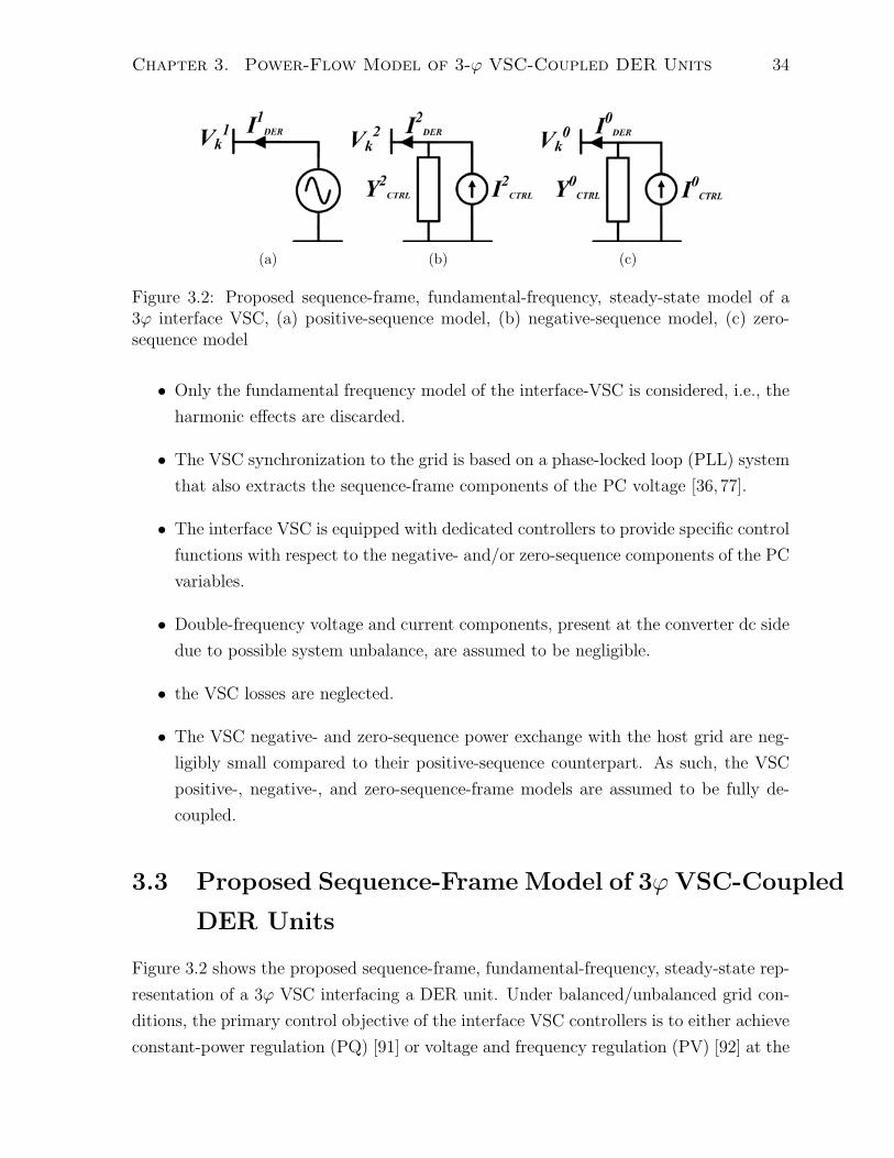
Figure 3.2: Proposed sequence-frame, fundamental-frequency, steady-state model of a3ϕ interface VSC, (a) positive-sequence model, (b) negative-sequence model, (c) zero-sequence model
• Only the fundamental frequency model of the interface-VSC is considered, i.e., the
harmonic effects are discarded.
• The VSC synchronization to the grid is based on a phase-locked loop (PLL) system
that also extracts the sequence-frame components of the PC voltage [36,77].
• The interface VSC is equipped with dedicated controllers to provide specific control
functions with respect to the negative- and/or zero-sequence components of the PC
variables.
• Double-frequency voltage and current components, present at the converter dc side
due to possible system unbalance, are assumed to be negligible.
• the VSC losses are neglected.
• The VSC negative- and zero-sequence power exchange with the host grid are neg-
ligibly small compared to their positive-sequence counterpart. As such, the VSC
positive-, negative-, and zero-sequence-frame models are assumed to be fully de-
coupled.
3.3 Proposed Sequence-Frame Model of 3ϕ VSC-Coupled
DER Units
Figure 3.2 shows the proposed sequence-frame, fundamental-frequency, steady-state rep-
resentation of a 3ϕ VSC interfacing a DER unit. Under balanced/unbalanced grid con-
ditions, the primary control objective of the interface VSC controllers is to either achieve
constant-power regulation (PQ) [91] or voltage and frequency regulation (PV) [92] at the
Chapter 3. Power-Flow Model of 3-ϕ VSC-Coupled DER Units 35
PC. This is realized by sensing the positive-sequence voltage and current components
at the PC, and utilizing them through a feedback process to control the coupling VSC
to generate the required positive-sequence voltage at its terminals. Thus, the positive-
sequence model of the VSC-coupled DER unit reflects either the PQ or the PV control
mode.
Should the DER unit be subjected to unbalanced power-flow, the negative- and/or
zero-sequence components of the PC variables also can be exploited to augment the
VSC switching process to provide specific control functions. For example, a three-wire
VSC can be controlled to inject (i) only balanced three-phase currents [36], or (ii) in
addition, a pre-specified amount of negative sequence current [37], to counteract the
system imbalance or for active islanding detection. If desired, a four-wire VSC can be
controlled also to compensate for the neutral (zero-sequence) current of a local unbalanced
three-phase load [35]. The developed negative- and zero-sequence frame VSC models in
this chapter are intended to reflect any/all of these VSC functionalities.
3.3.1 Interface VSC Positive-Sequence Model
The VSC positive-sequence model is similar to that of the TDSG shown in Fig. 2.2(a),
duplicated as Fig. 3.2(a) for ease of reference.
a) When the DER unit operates in the PV mode [92], its positive-sequence model with
respect to the PC is an ideal voltage source behind the PC bus. The specified volt-
age magnitude, |V1k|, at the PC and the positive-sequence real power injected (or
absorbed), P 1DER, by the unit are
|V1k| = Vsp, (3.1)
P 1DER =
Psp−DER
3, (3.2)
where Vsp and Psp−DER are the per-unit voltage and the three-phase real power refer-
ence set-points of the VSC.
b) When the DER unit is controlled to operate in the PQ mode, it is represented as a
constant power source. In this case, the real power injected/absorbed is given by (3.2)
and the exchanged reactive power, Q1DER, is
Q1DER =
Qsp−DER
3, (3.3)
where Qsp−DER is the per-unit three-phase reactive power reference set-point of the
Chapter 3. Power-Flow Model of 3-ϕ VSC-Coupled DER Units 36
VSC. In Fig. 3.2(a), I1DER is the positive-sequence current exchange between the DER
unit and the system.
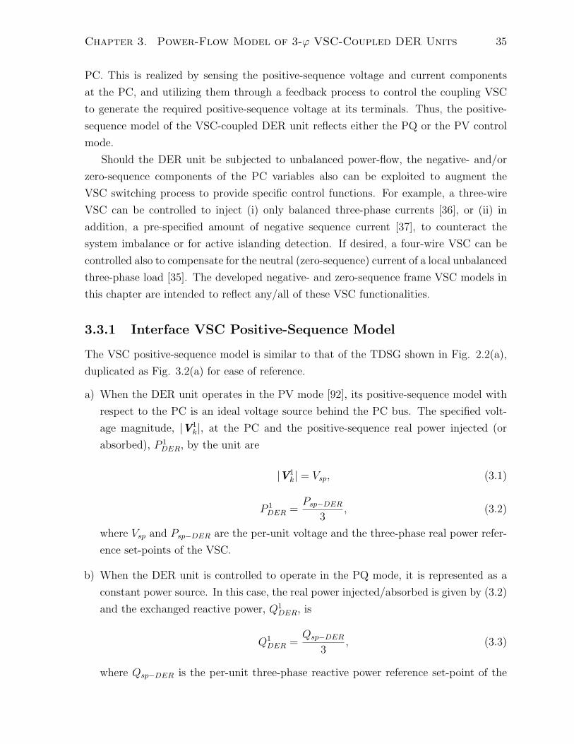
3.3.2 Interface VSC Negative- and Zero-Sequence Models
The negative- and zero-sequence models of the interface VSC are shown in Figs. 3.2(b)
and 3.2(c), respectively. A parallel combination of a current source (I0,2CTRL) and fictitious
admittance (Y0,2CTRL) can represent any control objective for both the three-wire and four-
wire VSC, corresponding to negative- and zero-sequence frames. In Fig. 3.2(b) (3.2(c)),
the net current exchange between the VSC negative- (zero-) sequence model and the
system is presented by I2DER(I0
DER).
3.3.2.1 Three-Wire VSC Configuration
If a three-wire interface-VSC is controlled only based on the positive-sequence dq current
control method [91], the DER unit also exchanges negative-sequence current with the
unbalanced system. In this case, the negative and zero sequence-frame components of
the model are specified as
I0,2CTRL = 0,
Y2CTRL = 1/Zf , (3.4)
Y0CTRL = 0,
where Zf is the equivalent series impedance of the VSC output filter between the PC
and the short-circuited VSC terminals. The VSC output filter is used to reduce the
harmonic current injected in the utility system [93]. The simplest output filter topology
is a series-connected inductor, Fig. 3.1, for which Zf is given by
Zf = Rf + jXf , (3.5)
where Xf/Rf is the VSC output filter net reactance/resistance. Other output filter
configurations are reported in [94]. These alternative configurations lie under either one
of the two topologies shown in Fig. 3.3. The equivalent series impedance, Zf , for the
Chapter 3. Power-Flow Model of 3-ϕ VSC-Coupled DER Units 37
(a) (b)
Figure 3.3: Alternative VSC output filter configurations
filter configurations shown in Fig. 3.3(a) and Fig. 3.3(b), is calculated as
Zf =Z1Z2
Z1 + Z2
, (3.6)
Zf = Z3 +Z1Z2
Z1 + Z2
, (3.7)
respectively, where Z1, Z2, and Z3 are shown in Fig. 3.3.
If a three-wire VSC is equipped with both positive- and negative-sequence current con-
trol schemes, and the negative-sequence current control is assigned to prevent negative-
sequence current exchange with the system [36], then the negative- and zero-sequence
models components are
I0,2CTRL = 0,
Y0,2CTRL = 0. (3.8)
For some applications, the negative-sequence controller of the three-wire VSC is de-
signed to inject a pre-specified negative-sequence current into the system, e.g., for island-
ing detection [37]. In this case, the negative and zero-sequence models of the interface-
VSC are
I2CTRL = INSCI � φNSCI ,
I0CTRL = 0, (3.9)
Y0,2CTRL = 0,
where INSCI and φNSCI are the magnitude and phase angle of the pre-specified negative
sequence current injection. In (3.4), (3.8), and (3.9), the parameters of the zero-sequence
model of Fig. 3.2(c) are always zero since there is no path for zero-sequence current flow.
Chapter 3. Power-Flow Model of 3-ϕ VSC-Coupled DER Units 38
3.3.2.2 Four-Wire VSC Configuration
The split-capacitor and the four-leg interface-VSC configurations can enable neutral con-
nection and establish a four-wire VSC system [35]. With respect to the steady-state
power-flow, both configurations are equivalent as long as the assumptions stated in Sec-
tion 3.2 are applicable. In addition to the positive-sequence current control, a four-wire
interface-VSC can exchange controlled negative- and zero-sequence current components
with the system, e.g., to counteract the imbalance due to unbalanced load at the PC [35].
The models of Fig. 3.2(b) and Fig. 3.2(c) can represent this strategy by setting
I0,2CTRL =
N∑i=1
V0,2i y0,2
BUS−ki− I0,2
load−k,
Y 0,2CTRL = 0, (3.10)
where I0,2load−k is the equivalent zero- and negative-sequence load current components
injected into the PC (Bus-k).
If the four-wire interface-VSC only injects a controlled positive-sequence current in the
system and permits the system to determine the exchanged negative- and zero-sequence
current components, then the corresponding model parameters are
I0,2CTRL = 0,
Y2CTRL =
1
Rf + jXf
, (3.11)
Y0CTRL =
1
(Rf + 3Rn) + j(Xf + 3Xn),
where Rn and Xn are defined in Fig. 3.1.
3.4 Implementation of the VSC Unified Model in the
SFPS
3.4.1 Accommodating the VSC-Coupled DER Model in the
SFPS
Consider a VSC-interfaced DER unit coupled to the host distribution network at Bus-k
(DER-k). To embed the model of Fig. 3.2 in the SFPS algorithm:
1. Add the terms Y0,2CTRL to the entries of the zero- and negative-sequence bus admit-
Chapter 3. Power-Flow Model of 3-ϕ VSC-Coupled DER Units 39
Figure 3.4: Equivalent sequence-frame circuits of a VSC-coupled DER unit
tance matrices corresponding to the kth row and the kth column (y0,2BUS−kk
), given
by (2.21), respectively.
2. Add the terms I0,2CTRL to the kth entries of the zero- and negative-sequence bus-
current injection vectors (I0,2BUS−k), given by (2.24), respectively.
3. Add the terms P 1DER and Q1
DER, given by (3.2) and (3.3), to the kth entry of the
specified real and reactive power vectors (P 1BUS−k and Q1
BUS−k), given by (2.25)
and (2.26), respectively.
3.4.2 Calculating the Internal Parameters of the Interface VSC
To impose the operating limits of the interface-VSC of DER-k in the SFPS, its internal
parameters values, i.e., modulation indices, phase currents, and reactive power (for PV
units), must be determined first. Figure 3.4 shows the equivalent sequence-frame circuits
of the interface VSC used to determine these parameters.
Subsequent to each power-flow iteration, the PC terminal conditions are evaluated.
The VSC net sequence-frame current components injected into the PC are
I0,2DER = I0,2
CTRL −Y0,2CTRLV 0,2
k� θ0,2
k , (3.12)
I1DER =
P 1DER − jQ1
DER
V 1k� − θ1
k
, (3.13)
where the elements of the VSC net current injection vector I012DER =
[I0
DER I1DER I2
DER
]′are specified on Fig. 3.2. Then the three-phase current Iabc
DER injected by the DER unit
is calculated using
IabcDER = TI012
DER, (3.14)
Chapter 3. Power-Flow Model of 3-ϕ VSC-Coupled DER Units 40
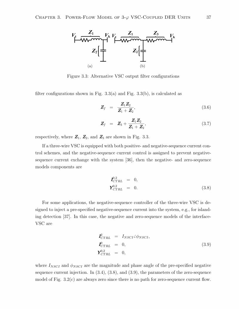
Table 3.1: VSC ConstantModulation Strategy Kinv
Sinusoidal Pulse 12√
2Width Modulation (SPWM)Space Vector 1√
6Modulation (SVM)
where the matrix T is given by (2.15) and
IabcDER =
[Ia
DER IbDER Ic
DER
]′. (3.15)
Finally, the sequence components of the interface-VSC terminal voltage, Fig. 3.4, can be
determined using
V 0,2t
� θ0,2t = I0,2
DER
(R0,2 + jX0,2
)+ V 0,2
k� θ0,2
k , (3.16)
V 1t� θ1
t =
(P 1
DER − jQ1DER
V 1k� − θ1
k
)(R1 + jX1
)+ V 1
k� θ1
k, (3.17)
where
R1,2 = Rf ,
R0 = Rf + 3Rn, (3.18)
X1,2 = Xf ,
X0 = Xf + 3Xn.
The VSC sequence- and phase-frame modulation indices are given by
m012 =V012
t
KinvVdc
, (3.19)
mabc = Tm012, (3.20)
where Kinv is the phase-to-neutral converter constant and is determined based on the
adopted modulation technique, as shown in Table 3.1 [95], and
mabc =[
ma � θat mb � θb
t mc � θct
]′, (3.21)
m012 =[
m0 � θ0t m1 � θ1
t m2 � θ2t
]′. (3.22)
Chapter 3. Power-Flow Model of 3-ϕ VSC-Coupled DER Units 41
3.4.3 Mitigating the VSC Operating Limits Violation
Subsequent to evaluating the internal parameters of the interface-VSC, its operating
limits are checked to achieve a power-flow solution that satisfies all the VSC’s constraints.
If any violation is detected, the voltage and/or power set points of each converter, i.e.,
Vsp, Psp−DER, and Qsp−DER, are updated based on the following proposed strategies.
3.4.3.1 Mitigating the Phase Current Limit Violation
If any of the DER phase currents (Ia,b,cDER) exceeds the maximum phase current limit, the
specified real and reactive power components associated with each VSC unit are updated
using
P 1DER,ct+1|x =
1
3Psp−DER,ct × Iph−max
max − violate(Ia,b,cDER−ct
) ,
Q1DER,ct+1|x =
1
3Qsp−DER,ct × Iph−max
max − violate(Ia,b,cDER−ct
) , (3.23)
where ct is the SFPS current iteration index and max−violate(Ia,b,cDER,ct
)is the magnitude
of the VSC largest violating phase current corresponding to iteration ct. Suffix x refers to
the VSC power set-points satisfying the VSC maximum current constraint. It should be
noted that if the DER unit is controlled to operate at a constant power-factor, then the
real and reactive power set-points are simultaneously updated using (3.23). Otherwise,
the DER reactive power contribution is reduced first to alleviate the violation while the
real-power set-point remains unaltered.
3.4.3.2 Mitigating the Reactive Power Limit Violation
For PV-controlled DER units, if the reactive power limit is hit, the specified positive
sequence voltage for the corresponding bus is updated using
Vsp,ct+1|y =
√Qmax × X1
cct
, (3.24)
where
cct =V 1
t,ct × cos(θ1
t,ct − θ1k,ct
)Vsp,ct
− 1. (3.25)
Equation (3.24) is the solution of (3.17) after replacing Q1 with Qmax and assuming
that R1 is much smaller than X1. Suffix y refers to the VSC voltage set-point satisfying
Chapter 3. Power-Flow Model of 3-ϕ VSC-Coupled DER Units 42
the maximum reactive power constraint.
It should be noted that, unlike the conventional N-R power-flow algorithms where
the violating PV bus is switched to PQ bus [72, 96, 97], the proposed approach of Sec-
tion 3.4.3.2 uses the closed form given by (3.24) and (3.25) to update the specified bus
voltage for the next iteration, Vsp,ct+1, such that the reactive power remains within the
acceptable operating limits. Consequently, the Jacobean matrix and states vector do not
require restructuring, corresponding to bus-type changing. This simplifies the algorithm
implementation and programming.
3.4.3.3 Mitigating the Phase Modulation Index Limit Violation
If any of the DER phase modulation indices (ma,b,c) exceeds the maximum phase modu-
lation index limit (mph−max), the following procedure is executed:
1. Set the violating modulation index equal to mph−max
2. Re-evaluate V 1t using (3.19) and (3.20)
3. Update P 1DER,ct+1|z and Q1
DER,ct+1|z (P 1DER|z and V 1
sp|z) for PQ (PV) units using
(3.17). Suffix z refers to the VSC set-points satisfying the maximum modulation
index constraint.
3.4.3.4 Updating the Interface VSC Reference Set-Points
The VSC reference set-points, selected prior to the (ct + 1)st power-flow iteration, must
satisfy all the aforementioned limits. As such, the VSC reference set-points (P 1DER,ct+1,
Q1DER,ct+1, Vsp,ct+1) are selected as:
P 1DER,ct+1 = min(P 1
DER,ct+1|x, P 1DER,ct+1|z, Psp−DER/3), (3.26)
Q1DER,ct+1 = min(Q1
DER,ct+1|x, Q1DER,ct+1|z, Qsp−DER/3) for PQ DER units,(3.27)
Vsp,ct+1 = min(Vsp,ct+1|y, Vsp,ct+1|z, Vsp) for PV DER units. (3.28)
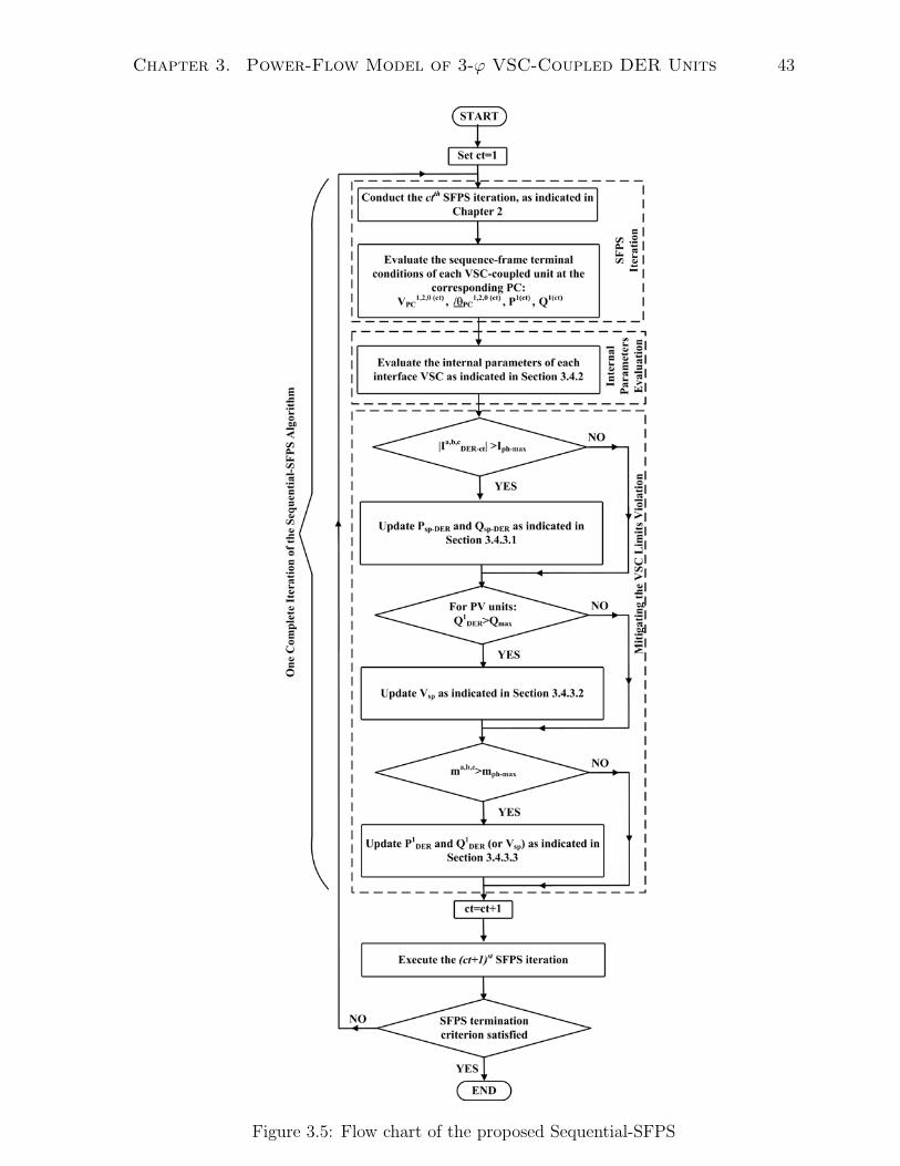
3.5 Sequential-SFPS
The procedures of Sections 3.4.2 and 3.4.3 are implemented as an interleaved step that
is iteratively executed subsequent to each SFPS iteration. The complete algorithm is
depicted in the flow chart of Fig. 3.5.
As seen from Fig. 3.5, the entire algorithm is decomposed into three main subroutines.
First, the system power-flow solution and the interface-VSC terminal conditions are
Chapter 3. Power-Flow Model of 3-ϕ VSC-Coupled DER Units 43
Figure 3.5: Flow chart of the proposed Sequential-SFPS
Chapter 3. Power-Flow Model of 3-ϕ VSC-Coupled DER Units 44
evaluated using the SFPS. Then, the interface-VSC internal currents and voltages are
calculated. Finally, the VSC reference set-points are updated to fulfil all the interface-
VSC’s constraints’ prior to proceeding to the next SFPS iteration. Thus, the algorithm
sequentially iterates between the SFPS and the updating algorithm. This is the reason
the term ”sequential” is emphasized for the proposed algorithm.
It should be noted that unlike the method presented in [32] and [34], where the
interface VSC constraints are evaluated after the final convergence of the power-flow
algorithm, the proposed method detects the violation once it occurs at any iteration of
the SFPS and automatically updates the VSC power and/or voltage set-points prior to
succeeding to the following power-flow iteration to ensure that all the constraints are
fulfilled. Hereafter, the method presented in [32] and [34] will be referred to as ”non-
sequential method”.
3.6 3ϕ VSC Model Validation
To evaluate the numerical accuracy of the proposed VSC models of Fig. 3.2 and verify
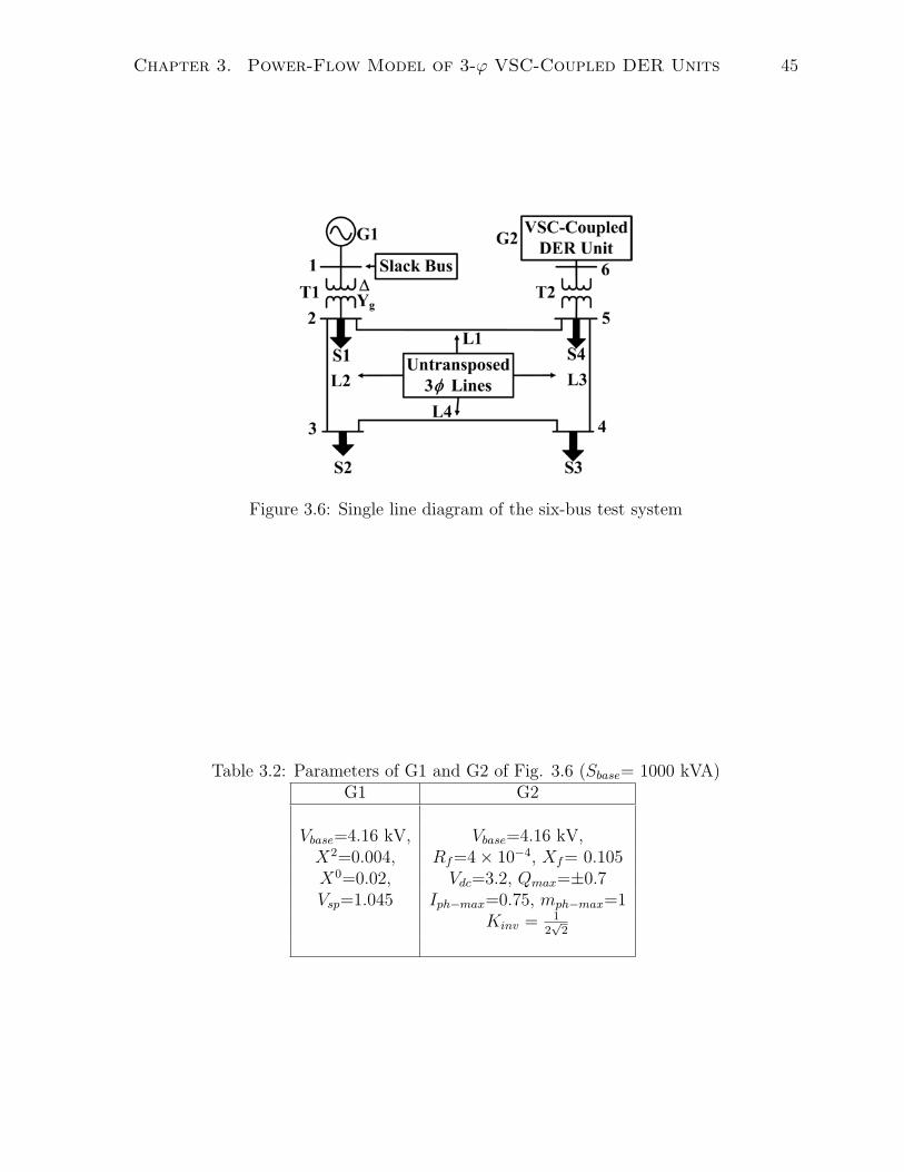
the validity of the Sequential-SPFS algorithm of Fig. 3.5, the six-bus study system of
Fig. A.1, duplicated as Fig. 3.6 for the ease of reference, is selected and four case stud-
ies (Case-1 to 4 ) are conducted. G1 is a voltage-controlled three-phase synchronous
generator with enough capacity to compensate the system slack, and is modeled as a
three-phase constant voltage source with negative and zero-sequence impedance. G2 is
a three-phase VSC-coupled DER unit, and is modeled as a controlled voltage source
behind the interface-VSC filter. As earlier stated in Chapter 1, the reason for selecting
this adequately small system is to be able to simulate the system in time-domain in the
PSCAD/EMTDC platform, and consequently, verifying the numerical accuracy of the
VSC models and the SFPS. The system parameters and loading profile are detailed in
Appendix A.1. The parameters of G1 and G2 are given in Table 3.2. Two applications of
the Sequential-SFPS to large distribution systems, with different R/X ratios and network
topologies, are presented in the next section.
To validate the proposed interface VSC model, the power-flow algorithm based on
the flow chart of Fig. 3.5, including the DER models of Section 3.3, is implemented
in the MATLAB® platform. The detailed model of the study system is also developed
in the PSCAD/EMTDC time-domain software to serve as the benchmark for valida-
tion of the interface-VSC model and the SPFS results. As discussed in Chapter 1, the
PSCAD/EMTDC simulation environment is selected since it contains detailed and widely
used time-domain models of power system components and allows incorporating various
Chapter 3. Power-Flow Model of 3-ϕ VSC-Coupled DER Units 45
Figure 3.6: Single line diagram of the six-bus test system
Table 3.2: Parameters of G1 and G2 of Fig. 3.6 (Sbase= 1000 kVA)G1 G2
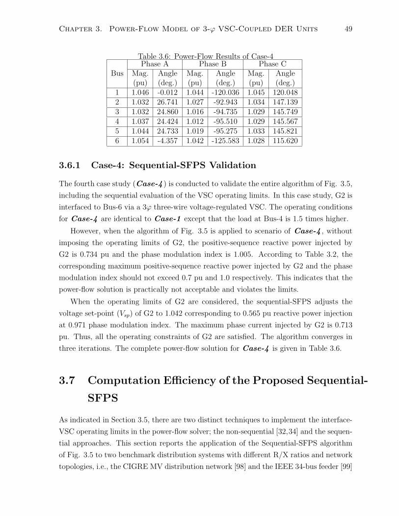
The fourth case study (Case-4 ) is conducted to validate the entire algorithm of Fig. 3.5,
including the sequential evaluation of the VSC operating limits. In this case study, G2 is
interfaced to Bus-6 via a 3ϕ three-wire voltage-regulated VSC. The operating conditions
for Case-4 are identical to Case-1 except that the load at Bus-4 is 1.5 times higher.
However, when the algorithm of Fig. 3.5 is applied to scenario of Case-4 , without
imposing the operating limits of G2, the positive-sequence reactive power injected by
G2 is 0.734 pu and the phase modulation index is 1.005. According to Table 3.2, the
corresponding maximum positive-sequence reactive power injected by G2 and the phase
modulation index should not exceed 0.7 pu and 1.0 respectively. This indicates that the
power-flow solution is practically not acceptable and violates the limits.
When the operating limits of G2 are considered, the sequential-SFPS adjusts the
voltage set-point (Vsp) of G2 to 1.042 corresponding to 0.565 pu reactive power injection
at 0.971 phase modulation index. The maximum phase current injected by G2 is 0.713
pu. Thus, all the operating constraints of G2 are satisfied. The algorithm converges in
three iterations. The complete power-flow solution for Case-4 is given in Table 3.6.
3.7 Computation Efficiency of the Proposed Sequential-
SFPS
As indicated in Section 3.5, there are two distinct techniques to implement the interface-
VSC operating limits in the power-flow solver; the non-sequential [32,34] and the sequen-
tial approaches. This section reports the application of the Sequential-SFPS algorithm
of Fig. 3.5 to two benchmark distribution systems with different R/X ratios and network
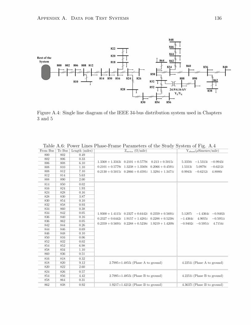
topologies, i.e., the CIGRE MV distribution network [98] and the IEEE 34-bus feeder [99]
Chapter 3. Power-Flow Model of 3-ϕ VSC-Coupled DER Units 50
to (i) verify the feasibility of the developed Sequential-SFPS for large and realistic size
power systems and (ii) demonstrate the convergence superiority of the proposed approach
compared to the non-sequential method [32,34]. The single-line diagrams and parameters
of both test systems are detailed in Appendix A.2 and Appendix A.4, respectively.
The 12.47 kV, three-phase, four-wire CIGRE distribution network of Fig. A.2 is
equipped with two DER units:
1. DER1 is a 3ϕ three-wire voltage-controlled VSC-coupled DER unit connected to
Bus-8 via a three-phase transformer (200 kVA, 12.47/4.16 kV, Yg/�) and is rated at
200 kVA, 4.16 kV. DER1 operates as a PV unit to maintain the positive-sequence
voltage component of its corresponding bus at 1 pu and inject 200 kW into the
network.
2. DER2 is a 3ϕ three-wire current-controlled VSC-coupled DER unit connected to
Bus-3 via a three-phase transformer (150 kVA, 12.47/4.16 kV, Yg/�). DER2 is
rated at 150 kVA, 4.16 kV. DER2 operates as a PQ unit to inject 150 kVA at
unity power-factor and inject 0.03 pu negative-sequence current for active islanding
detection [37].
The 24.9 kV, three-phase, four-wire IEEE 34-bus feeder of Fig. A.4 is equipped with
three VSC-coupled DER units:
1. DER3 is a 3ϕ four-wire current-controlled VSC-coupled DER unit connected to
Bus-814 via a three-phase transformer (100 kVA, 24.9/4.16 kV, Yg/Yg). DER3 is
rated at 100 kVA, 4.16 kV and operates as a PQ unit to inject 100 kVA at unity
power-factor and compensate for the unbalanced load currents at Bus-814.
2. DER4 and DER5 are 3ϕ three-wire voltage-controlled VSC-coupled DER units
connected to Bus-858 and Bus-836, respectively. Each unit is connected to the grid
via a three-phase transformer (100 kVA, 24.9/4.16 kV, Yg/�). Each unit is rated
at 100 kVA and 4.16 kV. Both units operate as PV units to maintain the positive-
sequence voltage component of their corresponding bus at 1.0 pu and inject 1.0 pu
active power into the network.
The internal parameters of the DER1-DER5 are the same as those of unit G2 of Table
3.2.
The non-sequential power-flow algorithm, reported in [32, 34], is implemented in the
MATLAB® platform. The sequential and the non-sequential programs are applied to
evaluate the power-flow solution of the CIGRE MV distribution network and the IEEE
34-bus feeder.
Chapter 3. Power-Flow Model of 3-ϕ VSC-Coupled DER Units 51
Figure 3.7: Comparison between the sequential and the non-sequential power-flow algo-rithms in terms of the convergence speed
Table 3.7: Comparison Between the Sequential and the Non-Sequential Power-Flow Al-gorithms in Terms of the Total Number of Jacobean Matrix Evaluations/Inversions
Test Proposed Non-sequentialSystem sequential-SFPS methodSix-bus
3 6test systemCIGRE MV
4 6distribution network
IEEE 34-bus7 15
feeder
The power-flow results of both algorithms favorably agree. Fig. 3.7 compares the
convergence speed of the two algorithms and indicate that the Sequential-SFPS provides
a superior convergence rate.
Another figure of merit of the Sequential-SFPS with respect to the non-sequential
approach is the number of evaluations/inversions of the Jacobian matrix to obtain the
power-flow solution, as shown in Table 3.7. The results of Fig. 3.7 and Table 3.7 are
based an Intel® Core2Duo™, 3.16 GHz processor. Figure 3.7 and Table 3.7 show that
the sequential-SFPS outperforms the non-sequential method.
The computational efficiency of the Sequential-SFPS, as compared to the non-sequential
method, is explained as follows. As indicated in Table 3.7, the Sequential-SFPS requires
less number of Jacobian matrix evaluations/inversions, which is the most time-consuming
part of the power-flow algorithm. In the proposed sequential approach, the VSC con-
straint evaluation of the DER units, and consequently updating the voltage and/or power
set-points, is formulated as an interleaved step with each SFPS iteration. Thus, the sub-
sequent power-flow iteration is not executed until all the VSC constraints are fulfilled.
Chapter 3. Power-Flow Model of 3-ϕ VSC-Coupled DER Units 52
However, the non-sequential method evaluates the DER constraints subsequent to the
convergence of the entire SFPS algorithm. This results in larger number of power-flow
iterations and Jacobian matrix evaluations/inversions, as compared to the Sequential-
SFPS.
3.8 Summary and Discussion
This chapter develops a unified sequence-frame-based, three-phase, fundamental-frequency
model for VSC-coupled DER units for balanced and unbalanced power-flow analysis. The
proposed model accommodates (i) both three-wire and four-wire VSC configurations, (ii)
various VSC control features/strategies, and (iii) the operating limits of the interface-
VSC, under balanced and unbalanced power-flow conditions.
This chapter also presents the necessary modifications to embed the unified model
in the SFPS. In contrast to the existing methods, the algorithm utilizes a sequential
iterative process with respect to the network and the VSC solutions to guarantee that
the power-flow solution adheres to the interface VSC constraints and operating limits.
Chapter 4
Power-Flow Model of Type-3 Wind
Generation Unit: Mathematical
Formulation1
4.1 Introduction
This chapter develops a comprehensive mathematical model of the Type-3 DER unit,
i.e., a doubly-fed asynchronous generator (DFAG) and its associated converter system,
for three-phase PFA using the SFPS. First, a sequence frame, steady-state, fundamental-
frequency model of a generic Type-3 DER unit is developed to represent (i) the control
capabilities and (ii) the operating limits of the rotor-side and the grid-side converters
under balanced and unbalanced power-flow conditions. New strategies to determine the
reference set-points of the controllers for compliance with the operating limits, are also
presented. The model, including the proposed strategies, is incorporated with SFPS. For
numerically accurate and computationally efficient solutions, the sequential approach,
proposed in Chapter 3, is used to impose the operating limits of the Type-3 DER unit.
Applications and validation of the developed model and the set-points update strategies,
and evaluation of the computational efficiency of the power-flow algorithm are covered
in Chapter 5.
1The work presented in this chapter has been accepted for publication, and will appear in M.Z. Kamhand R. Iravani, “Three-Phase Model and Power-Flow Analysis of Wind-Driven Doubly-Fed AsynchronousGenerators Part I: Model Development,” IEEE Trans. Sustainable Energy, April 2011, Manuscript IDTSTE-00186-2010.
53
Chapter 4. Power-Flow Model of Type-3 WTG DER Units 54
4.2 Classification of Wind Turbine Generators
Over the past two decades, wind energy has gained the most attention as a clean,
environmentally-friendly, and free source of electricity generation [53, 54, 100]. Wind
turbines generating units (WTGUs) are classified into three main categories:
• fixed speed units (Type-1 WTGUs)
• semi-variable speed units (Type-2 WTGUs)
• variable speed units (Type-3 and Type-4 WTGUs)
4.2.1 Type-1 WTGU
This category deploys the squirrel cage induction generator (SCIG) which is driven by
a wind turbine either having a fixed turbine blade angle (stall regulated fixed speed
WTGU) or having a pitch controller to regulate the blade angle (pitch regulated fixed
speed WTGU), Fig. 4.1(a) [100]. The rotor speed is almost fixed. Type-1 WTGUs
are directly connected to the grid via a step-up transformer. For rotor speeds higher
than the synchronous speed, the unit injects active power into the grid. Reactive power
compensation is provided to Type-1 generators through the grid and fixed shunt ca-
pacitors (for power factor correction purpose). The amount of real and reactive power
supplied/consumed by Type-1 WTGUs solely depend on the turbine and generator char-
acteristics, wind speed, and grid voltage.
4.2.2 Type-2 WTGU
Pitch controlled turbines and wound rotor induction generators (WRIG) are deployed in
this category. Rotor speed can be varied within a range of 10% using an electronically-
controlled variable resistor connected to the machine’s rotor, Fig. 4.1(b). Type-2 WTGUs
are directly connected to the grid via a step-up transformer. Reactive power compensa-
tion is identical to Type-1.
4.2.3 Type-3 WTGU
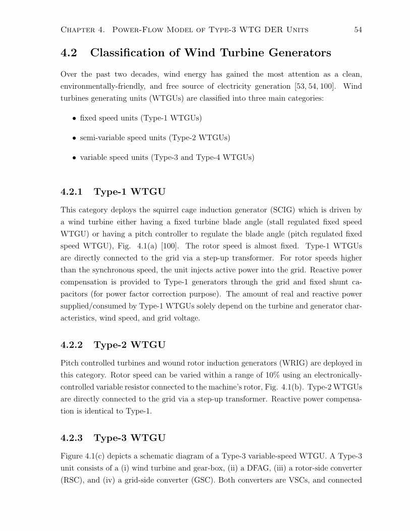
Figure 4.1(c) depicts a schematic diagram of a Type-3 variable-speed WTGU. A Type-3
unit consists of a (i) wind turbine and gear-box, (ii) a DFAG, (iii) a rotor-side converter
(RSC), and (iv) a grid-side converter (GSC). Both converters are VSCs, and connected
Chapter 4. Power-Flow Model of Type-3 WTG DER Units 55
(a)
(b)
(c)
(d)
Figure 4.1: Schematic diagrams of the four types of wind-turbine generating systems:(a) Type-1, (b) Type-2, (c) Type-3, and (d) Type-4
Chapter 4. Power-Flow Model of Type-3 WTG DER Units 56
using the back-to-back (B2B) configuration with a common DC link to operate as a
frequency-converter.
Among the four types of WTGUs, Type-3 WTGUs are the most deployed due to their
salient capabilities, i.e., (i) constant frequency/variable speed operation, (ii) independent
four-quadrant active and reactive power control, (iii) reactive power support, and (iv)
reduced converter ratings [101–103]. Hereafter, “Type-3” is used to refer to the DFAG,
RSC, GSC, and the DC link.
4.2.4 Type-4 WTGU
Variable-speed operation can also be achieved using direct-driven squirrel-cage induc-
tion/permanent magnet synchronous generator units with a full-scale B2B VSC to inter-
face the stator to the host grid, Fig. 4.1(d) [104]. For generators with large number of
poles, the gearbox may be eliminated to increase the overall system efficiency. Type-4
WTGU has the same advantage of the Type-3 units. However, the power-electronic con-
verter should be sized to overpass the full rating of the machine to provide the adequate
reactive power compensation [104].
4.3 Power-Flow Models of Type-3 DER Units: Re-
view
The existing WTGU steady-state models focus on Type-1 and Type-2 arrangements
[46,47,51–54,62,105]. While the DER model developed in Chapter 3 encompasses Type-
4 WTGU, the available Type-3 models neither consider the system unbalanced conditions
nor represent the unit operating limits [49,50].
In [50], a primitive steady-state Type-3 model is developed to assess the voltage
stability limits of electrical power systems, where PV bus with reactive power limits is
used to model voltage-regulated Type-3 units while constant PQ bus is used to model
power-factor controlled units. Such model can neither address the unbalanced operation
of the Type-3 unit nor the impacts of the power-electronic converters’ operating limits.
An iterative method is developed in [49] to consider the RSC current limits. However,
the model neither includes all the other Type-3 operational limits nor considered the
unbalanced grid conditions on the unit’s performance. The unbalanced models described
in [51] and [62] are developed in the sequence-components frame, but are only applicable
for fixed-speed wind-driven units. The impact of the operational limits of the interfacing
Chapter 4. Power-Flow Model of Type-3 WTG DER Units 57
power electronic converters should be considered for accurate modeling of the WTGUs
[106].
4.4 The Scope of the Chapter
The Type-3 WTGU is either connected to a distribution system as a single distributed
generation (DG) unit [107] or constitutes a WTGU of a large wind farm which is inter-
faced to a transmission system [108]. The former case is the main focus of this chapter.
As earlier emphasized in Chapter 2, distribution systems are inherently unbalanced. For
the scenario that a Type-3 WTGU is interfaced to a distribution system, the voltage
unbalance should be properly addressed and quantified for control and operation of the
unit. Unbalanced voltage at the Type-3 terminal can lead to erroneous tripping due to
excessive DFAG stator current unbalance, excessive rotor surface heating, and mechanical
damage as a result of power/torque oscillations [78].
The scope of this chapter is to develop a steady-state model and a PFA algorithm for
a generic Type-3 DER unit, operating as a DG unit under balanced/unbalanced network
conditions. Considering various control capabilities of Type-3 unit, the developed model
addresses:
• voltage/frequency (PV) control mode (in case of islanded operation [109]) or con-
stant power-factor or active/reactive power (PQ) controls (in the grid-connected
mode),
• specific control actions to mitigate the stator voltage unbalance impact [78–83],
• operational limits of the unit and its associated power-electronic converters, i.e.,
maximum positive- and negative-sequence currents and modulation indices.
The developed model can also be adopted for power-flow analysis and parameter/set-
point adjustment of a wind farm composed of Type-3 WTGUs. The equivalent steady-
state model of a Type-3 based wind farm, with respect to the wind farm point of con-
nection, for power-flow analysis of an interconnected power system is provided in [110]
and not discussed in this chapter.
Chapter 4. Power-Flow Model of Type-3 WTG DER Units 58
4.5 Proposed Sequence-Frame Model of A Type-3
DER Unit
This section extends the VSC model of Chapter 3 to develop a sequence-frame, steady-
state model of the Type-3 DER unit. The VSC positive-sequence model is a power/voltage
source, while the negative- or the zero-sequence counterpart comprises a shunt combina-
tion of (i) a controlled current source and (ii) a fictitious impedance.
4.5.1 Model Assumptions
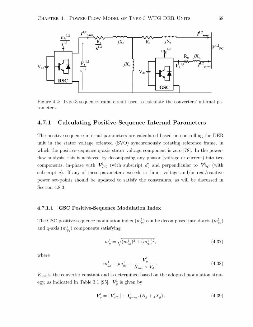
Figure 4.2 shows a schematic diagram of a Type-3 DER unit coupled to the host system
at the PC. The proposed Type-3 model is based on the following assumptions:
• The GSC controllers regulate the common DC-link voltage under steady-state con-
ditions.
• The double-frequency component of the DC-link voltage, due to the system unbal-
ance, is negligible.
• Only the fundamental-frequency model of the Type-3 is of interest, i.e., the har-
monic effects are discarded.
• The DER unit is synchronized to the grid using a phase-locked loop (PLL) system
that also extracts the sequence-components frame of the PC voltage [36].
• The RSC and/or GSC are equipped with dedicated controllers to provide specific
control functions with respect to the negative- and/or zero-sequence components
of the PC variables.
• the losses associated with RSC and GSC are neglected.
• The DER negative- and zero-sequence power exchange with the host grid are neg-
ligibly small compared to their positive-sequence counterpart. As such, the Type-3
WTG-based DER positive-, negative-, and zero-sequence-frame models are assumed
to be fully decoupled.
4.5.2 Positive-Sequence Model of Type-3 DER Unit
Under (un)balanced grid conditions, the RSC is primarily controlled to (i) extract the
maximum stator real power (Ps) at a given wind speed, and (ii) regulate the stator
Chapter 4. Power-Flow Model of Type-3 WTG DER Units 59
Figure 4.2: Detailed schematic diagram of a Type-3 wind-driven generation system
reactive power (Qs). This is realized by regulating the rotor real and reactive power
components (Pr, Qr), Fig. 4.2. At steady-state, (i)the GSC positive-sequence real power
set-point (Pg) is adjusted to exchange Pr with the grid. Depending on the control strategy,
(ii) the GSC reactive power is adjusted to provide reactive power support to regulate
either the power-factor or the stator terminal voltage [109]. In this work, the Type-
3 operates in the PQ (PV) mode if a constant reactive power/power-factor (terminal
voltage) is desired. Figure 4.3(a) shows the positive-sequence model of the Type-3 unit.
4.5.2.1 PV mode of operation
When the Type-3 DER unit operates in the PV mode [109], its positive-sequence model
with respect to the PC is an ideal voltage source behind the PC bus. The specified
voltage magnitude |V1PC | at the PC and the injected positive-sequence real power P 1
DER,
in per-unit, are
|V1PC | = Vsp, (4.1)
P 1DER =
Ps−spec + Pg−spec
3, (4.2)
where Vsp, and Ps−spec (Pg−spec) are the per-unit terminal voltage and three-phase stator
(GSC) real power reference set-points respectively. At steady-state, the relation between
Pg−spec, Pr−spec, and Ps−spec can be simplified to [111]
Pg−spec = −Pr−spec � −s1Ps−spec. (4.3)
Chapter 4. Power-Flow Model of Type-3 WTG DER Units 60
(a)
(b)
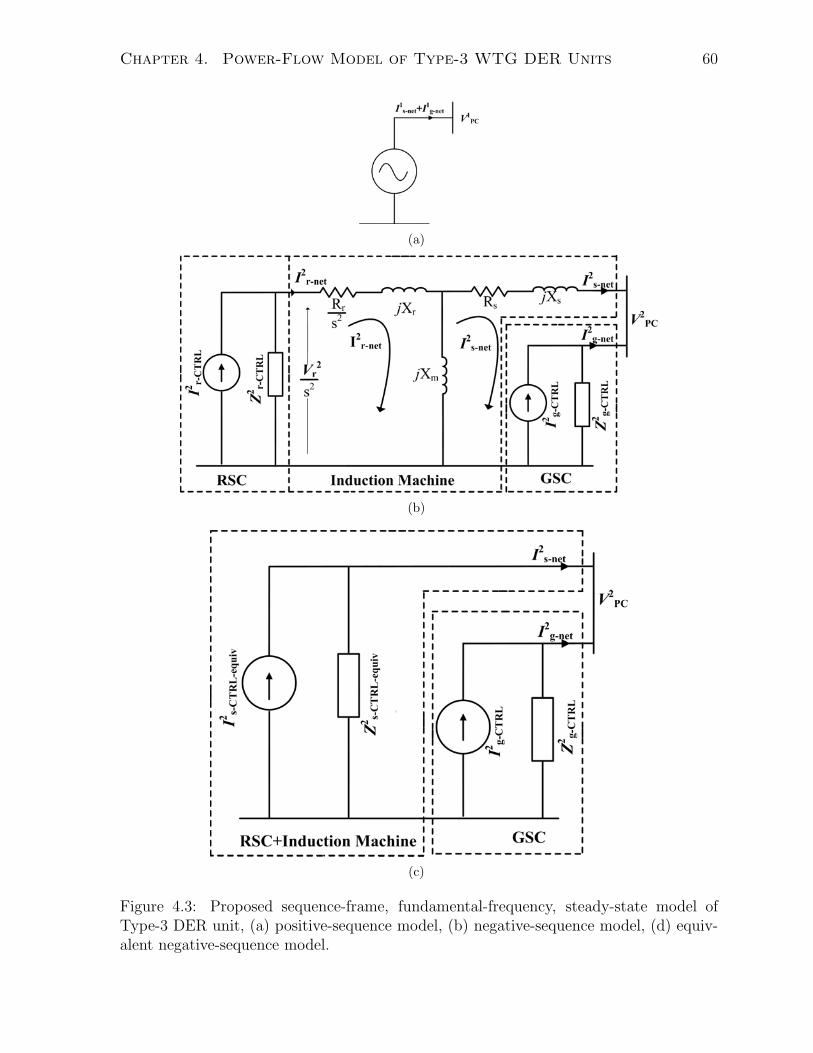
(c)
Figure 4.3: Proposed sequence-frame, fundamental-frequency, steady-state model ofType-3 DER unit, (a) positive-sequence model, (b) negative-sequence model, (d) equiv-alent negative-sequence model.
Chapter 4. Power-Flow Model of Type-3 WTG DER Units 61
In (4.3), s1 is the positive-sequence slip and is given by
s1 =ωs − ωr
ωs
, (4.4)
where ωs and ωr are the synchronous and rotor speeds, respectively.
4.5.2.2 PQ mode of operation
When the Type-3 unit is controlled in the PQ mode, it is represented as a constant power
source. In this case, the unit positive-sequence real power contribution is given by (4.2)
and the exchanged positive-sequence reactive power, Q1, is
Q1DER =
Qs−spec + Qg−spec
3. (4.5)
In Fig. 4.3(a), I1s−net/I
1g−net is the net positive-sequence current exchange between the
stator/ GSC and the PC bus.
4.5.3 Negative-Sequence Model of Type-3 DER Unit
As earlier discussed in Section 4.4, the unbalanced operation of a Type-3 unit is detri-
mental to its performance and lifetime [78]. The RSC and/or the GSC can be controlled
to inject negative-sequence currents to mitigate the effects of unbalanced stator voltage.
As discussed in Chapter 3, the VSC negative-sequence model is a parallel combination
of a current source (ICTRL) and an impedance (ZCTRL). Replacing the RSC and GSC
with this model yields the negative-sequence model of Fig. 4.3(b), where Rs (Xs) and Rr
(Xr) are the stator and rotor resistances (leakage reactances), Xm is the magnetizing re-
actance. I2r−CTRL, Z2
r−CTRL, I2g−CTRL, and Z2
g−CTRL are selected to realize the secondary
(negative-sequence) control objective. The negative-sequence slip, s2, is
s2 =ωs + ωr
ωs
= 2 − s1. (4.6)
4.5.4 Equivalent Negative-Sequence Model of Type-3 DER Unit
The negative-sequence model of Fig. 4.3(b) can be further simplified using the Norton cir-
cuit reduction technique, i.e., replacing the RSC and the asynchronous machine models,
shown in Fig. 4.3(b) inside the two leftmost dashed blocks, by an equivalent circuit con-
sisting of a current source (I2s−CTRL−equiv) in parallel with an impedance (Z2
s−CTRL−equiv),
Chapter 4. Power-Flow Model of Type-3 WTG DER Units 62
Fig. 4.3(c). Z2s−CTRL−equiv and I2
s−CTRL−equiv are given by (4.7) and (4.8), respectively.
Z2s−CTRL−equiv = Rs + jXs +
jXm ×(
Rr
s2 + jXr + Z2r−CTRL
)Rr
s2 + j(Xr + Xm) + Z2r−CTRL
(4.7)
I2s−CTRL−equiv =
I2r−CTRL × Z2
r−CTRL × jXm(Z2
r−CTRL + Rr
s2 + jXr + jXm×(Rs+jXs)Rs+j(Xs+Xm)
)(Rs + j(Xs + Xm))
(4.8)
It should be noted that the zero-sequence model of the Type-3 unit is not required
since it is typically connected in delta or an un-grounded-Wye, and thus does not permit
the flow of zero-sequence current [62].
The next section describes the secondary control objectives that can be achieved
by the GSC/RSC controllers. Moreover, it provides the appropriate values of I2r−CTRL,
Z2r−CTRL, I2
g−CTRL, Z2g−CTRL, I2
s−CTRL−equiv, and Z2s−CTRL−equiv to realize these objectives.
4.6 Evaluating Type-3 Negative-Sequence Model Pa-
rameters
The RSC and/or the GSC can be controlled to provide secondary control objectives under
unbalanced conditions. These may include:
1. Balancing the rotor currents.
2. Balancing the stator currents.
3. Mitigating the stator real power double-frequency component.
4. Mitigating the electromagnetic torque/power double-frequency oscillations to pre-
vent rotor mechanical stresses.
5. Mitigating the double-frequency components of the electromagnetic torque/power
and the unit net real power contribution (Ps + Pg) double-frequency component.
A combination of these control objectives can be realized by either the RSC [78–80],
the GSC [81], or their coordinated operation [82,83]. This section deduces the parameters
of the Type-3 unit negative-sequence model, Figs. 4.3(b) and 4.3(c), to include the impact
of these control strategies on the power-flow analysis which is dominantly determined by
the positive-sequence model of Fig. 4.3(a).
Chapter 4. Power-Flow Model of Type-3 WTG DER Units 63
4.6.1 Case A: Idle Secondary Control of Type-3 Unit
If both the RSC and the GSC are controlled only based on the positive-sequence dq-
current control method [91], the DER unit will exchange negative-sequence current with
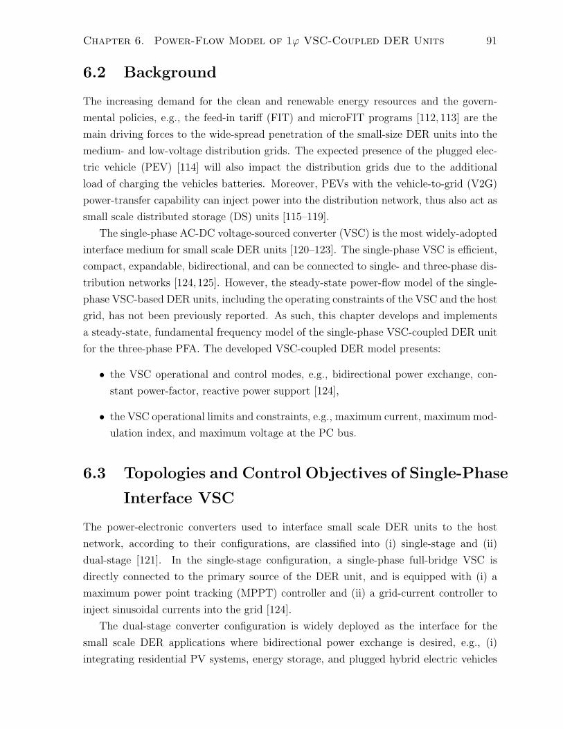
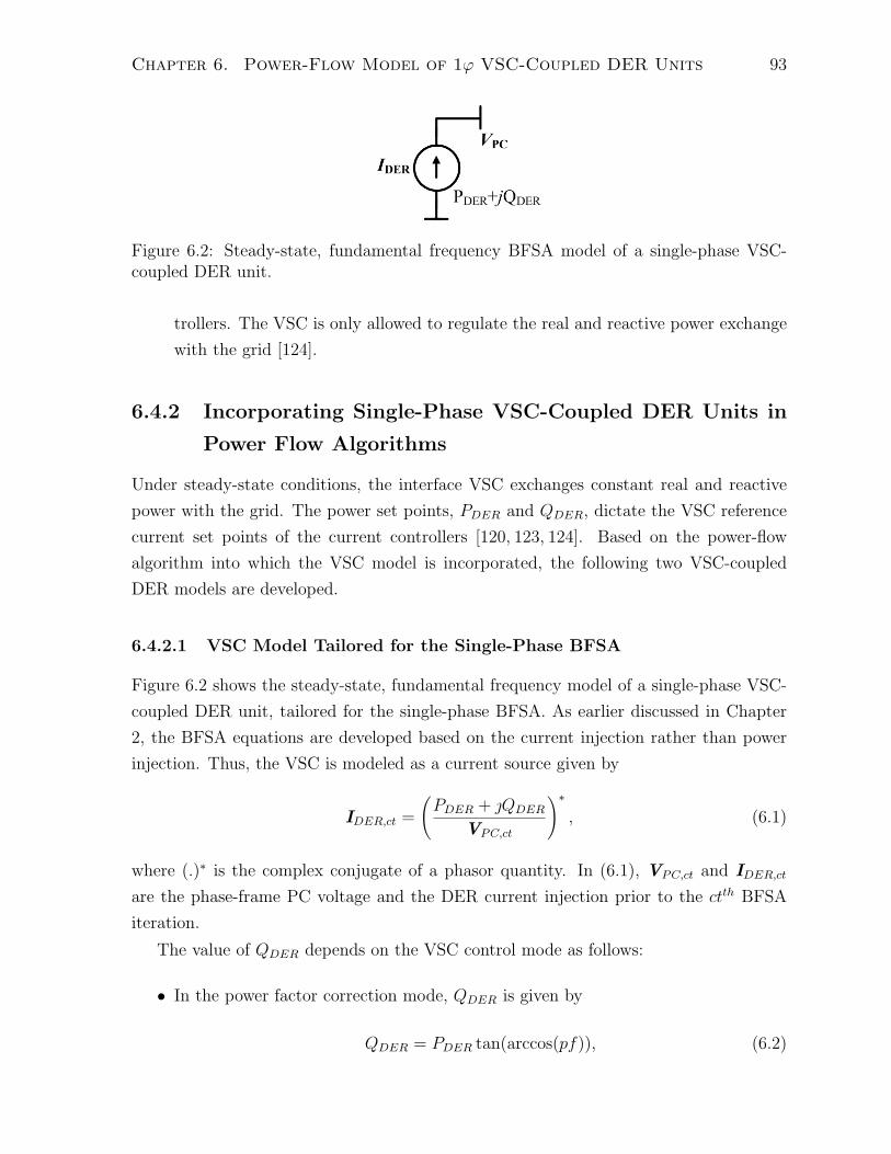
the unbalanced grid. In this case (i) I2r−CTRL, Z2
r−CTRL, and I2g−CTRL are all set to zero,
and (ii) I2s−CTRL−equiv and Z2
s−CTRL−equiv are determined by (4.7) and (4.8) respectively.
Z2g−CTRL is given by
Z2g−CTRL = Rg + jXg, (4.9)
where Rg and Xg are defined on Fig. 4.2.
4.6.2 Case B: Balancing Rotor Currents
The negative-sequence control capability of the RSC can be used to prevent the negative-
sequence current flow in the rotor windings [78], [79], and [80]. The impact of this
control scenario on the steady-state power-flow is determined by setting I2r−CTRL = 0
and imposing Z2r−CTRL = ∞. As a result, I2
s−CTRL−equiv = 0, and by applying L’Hopital
rule to (4.7),
Z2s−CTRL−equiv = Rs + j(Xs + Xm). (4.10)
In addition, if the GSC is controlled to block its negative-sequence current exchange
with the PC bus, then
I2g−CTRL = 0, (4.11)
Z2g−CTRL = ∞. (4.12)
Otherwise, Z2g−CTRL is given by (4.9).
4.6.3 Case C: Balancing Stator Currents
The Type-3 unit can be controlled to block the negative-sequence stator current. This is
realized by controlling the RSC [78], [79], and [80] or the GSC [81] individually.
4.6.3.1 Case C-1: Balancing Stator Currents Via RSC
Applying the Kirchhoff’s voltage law to the stator circuit of Fig. 4.3(b), while neglecting
the stator resistance voltage drop, yields
−j(Xs + Xm)I2s−net + jXmI2
r−net = V2PC . (4.13)
Chapter 4. Power-Flow Model of Type-3 WTG DER Units 64
Thus, the negative-sequence stator current I2s−net can be eliminated by controlling the
RSC to inject a net negative-sequence rotor current I2r−net, where
I2r−net =
V 2PC
jXm
. (4.14)
This is realized by setting
Z2r−CTRL = ∞, (4.15)
I2r−CTRL =
V2PC
jXm
. (4.16)
Consequently, Z2s−CTRL−equiv is given by (4.10) and I2
s−CTRL−equiv is given by
I2s−CTRL−equiv =
V2PC
Rs + j(Xs + Xm). (4.17)
4.6.3.2 Case C-2: Balancing Stator Currents Via GSC
The GSC is controlled to force a balanced stator current [81]. At steady-state, applying
Kirchhoff’s current law at the stator bus (bus-PC ) yields
I2s−net + I2
g−net + I2load−PC =
N∑i=1
V2iy
2PC−i
, (4.18)
where I2load−PC is the injected negative-sequence current corresponding to the loads at
the stator bus, V2i is the negative-sequence voltage at bus-i, y2
PC−iis the the negative-
sequence admittance matrix entry corresponding to the PCth row and the ith.
Consequently, the stator current can be balanced by setting Z2g−CTRL = ∞ and
I2g−CTRL =
N∑i=1
V2iy
2PC−i
− I2load−PC . (4.19)
For this case, the parameters of the RSC negative-sequence model, Figs. 4.3(b) and
4.3(c), are
Z2s−CTRL−equiv = ∞, (4.20)
I2s−CTRL−equiv = 0, (4.21)
Z2r−CTRL = I2
r−CTRL = 0, (4.22)
Chapter 4. Power-Flow Model of Type-3 WTG DER Units 65
It should be noted that this scenario is unique since Z2s−CTRL−equiv and I2
s−CTRL−equiv
are not evaluated using (4.7) and (4.8), but instead selected based on (4.20) and (4.21),
respectively.
4.6.4 Case D: Mitigating Stator Real Power Double-Frequency
Component
The stator real power is
Ps = �(3VPCI∗s−net
). (4.23)
However, since a space phasor, e.g., F, can be decomposed into two oppositely and
synchronously rotating space vectors F1 and F2 [78], i.e.,
F = F1 + F2e−j2ωst. (4.24)
Thus, (4.23) can be expressed
Ps = �(V1
PC(I1s−net)
∗ + V2PC(I2
s−net)∗)+ �
(V1
PC(I2s−net)
∗ej2ωst)
+ �(V2
PC(I1s−net)
∗e−j2ωst)
, (4.25)
where the double-frequency stator power (Ps−2ωst) is the sum of the last two terms in
(4.25). Ps−2ωst can be eliminated by controlling the RSC to inject a negative-sequence
stator current (I2s−net) that satisfies (4.26) and (4.27).
�(V1
PC(I2s−net)
∗ + V2PC(I1
s−net)∗) = 0, (4.26)
�(V1
PC(I2s−net)
∗ −V2PC(I1
s−net)∗) = 0, (4.27)
where �(.) and �(.) are the real and imaginary parts of a complex quantity, respectively.
Solving (4.26) and (4.27) simultaneously yields
I2s−net = −V2
PC (Ps−spec + jQs−spec)
3|V1PC |2
, (4.28)
where |V1PC | is the magnitude of the positive-sequence stator voltage. Equation (4.28) is
used to calculate the following model parameters of Figs. 4.3(b) and 4.3(c) to guarantee
Chapter 4. Power-Flow Model of Type-3 WTG DER Units 66
ripple-free stator output power
Z2r−CTRL = ∞ , (4.29)
I2r−CTRL =
I2s−net (Rs + jXs + jXm) + V2
PC
jXm
, (4.30)
From (4.29) and (4.30), I2s−CTRL−equiv is
I2s−CTRL−equiv = I2
s−net +V2
PC
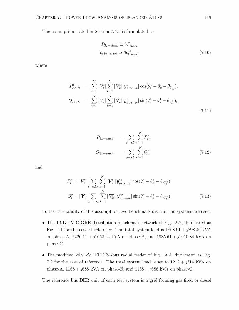
Rs + jXs + jXm
, (4.31)
where I2s−net is given by (4.28) and Z2
s−CTRL−equiv is given by (4.10).
4.6.5 Case E: Mitigating Double-Frequency Electromagnetic Torque
(Power) Component
Mitigating the double-frequency component in the electromagnetic power of Type-3 unit
is equivalent to eliminating the corresponding component in the stator reactive power
(Qs) [78–80,82,83]. Similar to the analysis of Section 4.6.4, this is realized by controlling
the RSC to inject a negative-sequence stator current component (I2s−net) to impose
�(V1
PC(I2s−net)
∗ + V2PC(I1
s−net)∗) = 0, (4.32)
�(V1
PC(I2s−net)
∗ −V2PC(I1
s−net)∗) = 0. (4.33)
From (4.32) and (4.33), I2s−net is deduced as
I2s−net =
V2PC (Ps−spec + jQs−spec)
3|V1PC |2
. (4.34)
Equations (4.29)-(4.31) are then used to evaluate the parameters of the Type-3 DER
negative-sequence model, Figs. 4.3(b) and 4.3(c).
4.6.6 Case F: Coordinated Control of GSC and RSC
GSC and RSC can be simultaneously controlled to (i) mitigate the double-frequency
electromagnetic power/torque component and (ii) dampen the associated real power
oscillations (Ps−2ωst + Pg−2ωst) [82, 83]. The first objective is realized via the RSC as
discussed in Section 4.6.5. To achieve the second objective, the GSC is controlled to
inject a negative-sequence current component (I2g−net) that cancels out the summation of
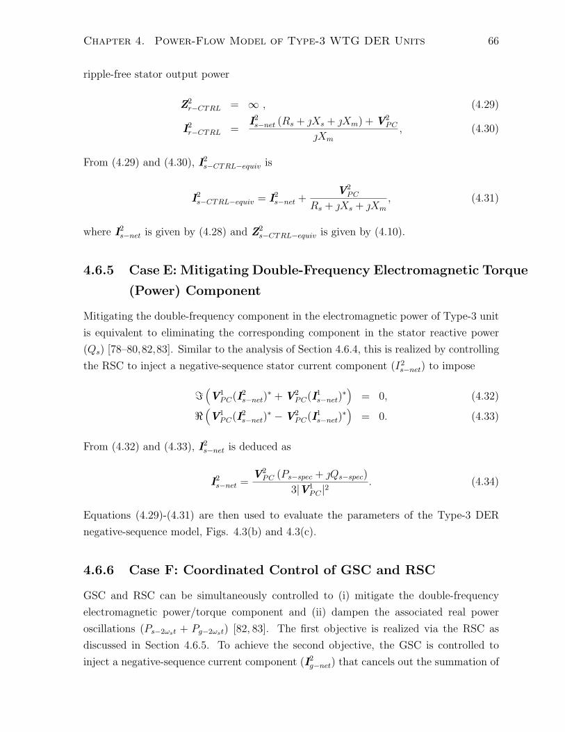
Chapter 4. Power-Flow Model of Type-3 WTG DER Units 67
Table 4.1: Parameters of the Type-3 Negative-Sequence Model For the Six Cases ofSection 4.6
Case A B C-1 C-2 D E FI2
r−CTRL 0 0 Eq. (4.16) 0 Eq. (4.28) and Eq. (4.30) Eq. (4.34) and Eq. (4.30) Eq. (4.34) and Eq. (4.30)Z2
r−CTRL 0 ∞ ∞ 0 ∞ ∞ ∞I2
s−CTRL−equiv 0 0 Eq. (4.17) 0 Eq. (4.28) and Eq. (4.31) Eq. (4.34) and Eq. (4.31) Eq. (4.34) and Eq. (4.31)
The Type-3 negative-sequence operating limits are fulfilled by adjusting the RSC and/or
GSC negative-sequence current injections (I2g−CTRL, I2
s−CTRL−equiv) as follows.
Subsequent to the ctth power-flow iteration, if m2ct
g > m2g−max, set m2ct
g = m2g−max and
update I2ct
g−CTRL|e using (4.54)-(4.56). Suffix e is used to define the GSC current injection
that satisfies the m2g limit.
Similarly, if |I2ct
g−net| > I2g−net−max, set |I2ct
g−net| = I2g−max and use it to update I2ct+1
g−CTRL|fusing (4.56). Suffix f refers to the GSC current injection that satisfies the |I2
g−net| limit.
The GSC negative-sequence current injection used in the (ct+1)st iteration is selected
as
I2ct+1
g−CTRL = min(I2ct+1
g−CTRL|e, I2ct+1
g−CTRL|f ). (4.76)
Using (4.57)-(4.59), the same procedure is followed to specify I2ct+1
s−CTRL.
4.8.4 Sequential SPFS
Subsequent to evaluating the internal parameters of TYPE3−k, the corresponding op-
erating limits are checked, and updated if necessary, to ensure no violations occur. The
steps to determine the internal parameters, evaluate the operating limits, and update the
DER reference set-points are performed sequentially at the end of each power-flow iter-
ation. A flow chart of the Sequential-SFPS, accommodating the Type-3 DER operating
Chapter 4. Power-Flow Model of Type-3 WTG DER Units 76
Figure 4.5: Flow chart of the proposed Sequential-SFPS algorithm including the Type-3DER constraints evaluation and the proposed reference-set point updating strategies
Chapter 4. Power-Flow Model of Type-3 WTG DER Units 77
limits, is shown in Fig. 4.5.
4.9 Summary and Discussion
This chapter introduces a comprehensive, sequence-frame based, three-phase, fundamental-
frequency, steady-state model of the Type-3 DER unit. The developed model can be
adopted for (i) power-flow analysis, (ii) determination of the operating limits, and (iii)
reference set-points adjustment of the Type-3 DER under balanced and unbalanced grid
conditions. The developed model is intended for steady-state/power-flow analysis of a
Type-3 unit that is utilized as a DER unit and interfaced to a distribution system. How-
ever, it can also be used for steady-state and power-flow analysis within a wind farm that
is composed of Type-3 units.
This chapter also incorporates the developed Type-3 sequence-frame model in the
SFPS. Subsequent to each power-flow iteration, the internal parameters of the Type-
3 unit are calculated. If any of the parameters violate the corresponding limits, the
positive- and/or negative-sequence reference set-points of the corresponding Type-3 unit
are updated prior to proceeding to the next power-flow iteration. Thus, the developed
algorithm sequentially iterates between the power-flow of the AC network and the Type-
3 unit to obtain a feasible power-flow solution. The applications and verification of the
developed Type-3 model and the power-flow algorithm are presented in Chapter 5.
Chapter 5
Power-Flow Model of Type-3 Wind
Generation Unit: Model Validation
and Applications1
5.1 Introduction
This chapter presents the implementation and validation of the steady-state, fundamental-
frequency, sequence-frame model of the Type-3 DER unit, accommodated within the
Sequential-SFPS algorithm, developed in Chapter 4. A set of case studies are reported to
(i) validate the numerical accuracy of the developed model and the power-flow algorithm,
(ii) quantify the impact of the Type-3 control strategy on the steady-state three-phase
power-flow solution, and (iii) demonstrate the computational efficiency of the Sequential-
SFPS with the imbedded Type-3 model. Three test systems of different topologies, sizes,
and parameters are examined. Where applicable the results are validated based on com-
parison with the exact time-domain solution, using the PSCAD/EMTDC simulation
platform.
5.2 Type-3 DER Model Validation
To evaluate the numerical accuracy of the proposed Type-3 DER model, accommodated
within the Sequential-SPFS algorithm of Chapter 4, the six-bus study system of Fig. A.1,
1The work presented in this chapter has been submitted for publication, and is in revision, in M.Z.Kamh and R. Iravani, “Three-Phase Model and Power-Flow Analysis of Wind-Driven Doubly-Fed Asyn-chronous Generators Part II: Validation and Applications,” IEEE Trans. Sustainable Energy, in Revi-sion, Nov. 2010, Manuscript ID TSTE-00187-2010.R1
78
Chapter 5. Applications and Validation of Type-3 WTG DER Model 79
Figure 5.1: Single line diagram of the six-bus test system
Table 5.1: Parameters of G2 of Fig. 5.1 (Sbase= 1000 kVA)G2
of both test systems are detailed in Appendix A.2 and Appendix A.4, respectively.
5.4.1 Case 7: CIGRE MV Distribution Network
The 12.47 kV, three-phase, four-wire CIGRE distribution network of Fig. A.2 is equipped
with two Type-3 DER units:
1. DER1 represents a voltage-controlled Type-3 DER unit (PV bus) connected to
Bus-8 via a three-phase transformer (150 kVA, 12.47/2.3 kV, Yg/�), and is con-
trolled to maintain the positive-sequence component of its terminal voltages at 1
pu while delivering 100 kW into the network. In addition to the positive-sequence
controllers, DER1 is controlled to balance the stator current via auxiliary GSC
negative-sequence current controllers. The GSC of DER1 is controlled to block the
negative-sequence GSC current exchange with the grid.
2. DER2 is a PQ unit that delivers 100 kW at unity power-factor, and is connected
to Bus-3 via a three-phase transformer (100 kVA, 12.47/2.3 kV, Yg/�). Moreover,
DER2 is equipped with additional controllers to mitigate the double-frequency
torque oscillations.
The three-phase voltage profile of the CIGRE distribution network, obtained using
the Sequential-SFPS algorithm, is depicted in Fig. 5.2. The operating constraints of
all the DER units are satisfied. This verifies the feasibility of the Sequential-SFPS for
non-radial ADN applications. The power-flow program converges in 0.264 seconds (3
iterations) using an Intel® Core2Duo™, 3.16 GHz processor, personal computer.
Chapter 5. Applications and Validation of Type-3 WTG DER Model 87
Figure 5.2: Voltage profile of the CIGRE distribution network with 2 Type-3 based DERunits
5.4.2 Case 8: IEEE 34-Bus Test System
In this case study, the 24.9 kV, three-phase, four-wire IEEE 34-bus feeder of Fig. A.4 is
equipped with three Type-3 DER units:
1. DER3 and DER4 are PV controlled units controlled to maintain the positive-
sequence voltage of the respective buses (Bus-814 and Bus-858 respectively) at
1 pu while injecting 100 kW power into the network. Each of these two units is
connected to the grid via a three-phase transformer (100 kVA, 24.9/2.3 kV, Yg/�).
Moreover, DER3 is equipped with auxiliary controllers to balance its rotor and
GSC currents simultaneously.
2. DER5 is connected to Bus-836 via a three-phase transformer (100 kVA, 24.9/2.3
kV, Yg/�), and is controlled to inject 100 kVA at unity power-factor.
Fig. 5.3 shows the three-phase voltage profile of the IEEE 34-bus distribution feeder.
The operating constraints of all the DER units are satisfied. This verifies the feasibility
of the Sequential-SFPS for radial ADN applications. The power-flow program converged
in 0.824 seconds (4 iterations) using an Intel® Core2Duo™, 3.16 GHz processor, personal
computer.
It should be noted that the computational time of Case-7 and Case-8 is larger than
that reported in Section 3.7. The reason is that the number of Type-3 DER constraints
evaluated subsequent to each power-flow iteration are much more than those of a VSC-
coupled DER unit. However, the convergence speed of the Sequential-SFPS, equipped
Chapter 5. Applications and Validation of Type-3 WTG DER Model 88
Figure 5.3: Voltage profile of the IEEE 34-bus distribution feeder with 3 Type-3 basedDER units
with the Type-3 model, is still acceptable for both test systems and could be even further
improved using the parallel programming techniques [73], which is beyond the scope of
this work.
5.5 Convergence Analysis
To further demonstrate the acceptable convergence behavior of the proposed algorithm,
regardless of the system parameters and topology, its convergence pattern is studied
for the three test systems. The value of the algorithm termination criterion (maximum
power mismatch) is changed and the corresponding number of iterations required by the
algorithm to converge is recorded. The algorithm convergence pattern is depicted in Fig.
5.4.
Figure 5.4 concludes that, regardless the system parameters and topology, the number
of iterations saturates when the termination criterion is reduced to 0.001 pu. This indi-
cates that the power mismatch is effectively reduced to a level less than the termination
criterion value in less than or equal to four iterations. This verifies that the computa-
tional efficiency of the proposed algorithm is independent of the network topology (mesh,
radial, or radial with loops) and parameters (X/R ratio).
5.6 Summary and Discussion
This chapter presents the applications and validation of (i) the steady-state sequence-
frame-based model of a Type-3 DER unit of Chapter 4, (ii) the computational efficiency
Chapter 5. Applications and Validation of Type-3 WTG DER Model 89
Figure 5.4: Convergence pattern of the Sequential-SFPS algorithm accommodating theType-3 DER
of the Sequential-SFPS accommodating the proposed model, and (iii) the feasibility of the
power-flow solver for large distribution networks. The developed DER model takes into
account all the control features and the operating limits of its power-electronic converters
under balanced and unbalanced power-flow conditions.
The proposed DER model is integrated with the Sequential-SFPS , implemented in
MATLAB®, and applied to three test systems of different sizes (six, eleven, and thirty-
four bus systems), topologies (mesh, and radial), and parameters (low, medium, and high
X/R ratios). Several case studies are conducted and where applicable, the results are
compared and validated against those obtained via time-domain simulations using the
PSCAD/EMTDC software. The results demonstrate:
• the numerical accuracy of the proposed Type-3 DER model,
• the impact of the Type-3 unit negative-sequence control strategy on the distribution
system power-flow results,
• the accuracy and computational efficiency of the Sequential-SFPS power-flow algo-
rithm irrespective of the network topology and parameters,
• feasibility of the power-flow solver for large distribution networks.
Chapter 6
Power-Flow Model of Single-Phase
VSC-Coupled DER Units1
6.1 Introduction
This chapter presents the steady-state, fundamental-frequency model of a DER unit
which utilizes a single-phase VSC as the interface medium. The model represents (i)
different operating and control modes and (ii) the operational constraints and limits of
the VSC and the host system, e.g., maximum current, maximum modulation index, and
maximum voltage at the point of connection (PC). The model is tailored for the PFA of
(i) three-phase distribution networks using the SFPS of Chapter 2 and (ii) single-phase
radial laterals, widely spread in the North-American distribution systems, using the well-
established Backward-Forward Sweep Algorithm (BFSA). The interface-VSC operating
limits are modeled and imposed on the power-flow solution using the sequential approach,
presented in Chapters 3 and 4, to increase the computational efficiency of the PFA tool.
Case studies are conducted to evaluate and verify (i) the accuracy of the proposed model
and (ii) the computational efficiency of the sequential method to handle the constraints
of the single-phase VSC.
1The work presented in this chapter has been submitted for publication, and is in revision, in M.Z.Kamh and R. Iravani, “Steady State Model and Power-Flow Analysis of Single-Phase Electronically-Coupled Distributed Energy Resources,” IEEE Trans. Power Delivery, in Revision, Jan. 2011,Manuscript ID TPWRD-00003-2011.R1
90
Chapter 6. Power-Flow Model of 1ϕ VSC-Coupled DER Units 91
6.2 Background
The increasing demand for the clean and renewable energy resources and the govern-
mental policies, e.g., the feed-in tariff (FIT) and microFIT programs [112, 113] are the
main driving forces to the wide-spread penetration of the small-size DER units into the
medium- and low-voltage distribution grids. The expected presence of the plugged elec-
tric vehicle (PEV) [114] will also impact the distribution grids due to the additional
load of charging the vehicles batteries. Moreover, PEVs with the vehicle-to-grid (V2G)
power-transfer capability can inject power into the distribution network, thus also act as
small scale distributed storage (DS) units [115–119].
The single-phase AC-DC voltage-sourced converter (VSC) is the most widely-adopted
interface medium for small scale DER units [120–123]. The single-phase VSC is efficient,
compact, expandable, bidirectional, and can be connected to single- and three-phase dis-
tribution networks [124, 125]. However, the steady-state power-flow model of the single-
phase VSC-based DER units, including the operating constraints of the VSC and the host
grid, has not been previously reported. As such, this chapter develops and implements
a steady-state, fundamental frequency model of the single-phase VSC-coupled DER unit
for the three-phase PFA. The developed VSC-coupled DER model presents:
• the VSC operational and control modes, e.g., bidirectional power exchange, con-
stant power-factor, reactive power support [124],
• the VSC operational limits and constraints, e.g., maximum current, maximum mod-
ulation index, and maximum voltage at the PC bus.
6.3 Topologies and Control Objectives of Single-Phase
Interface VSC
The power-electronic converters used to interface small scale DER units to the host
network, according to their configurations, are classified into (i) single-stage and (ii)
dual-stage [121]. In the single-stage configuration, a single-phase full-bridge VSC is
directly connected to the primary source of the DER unit, and is equipped with (i) a
maximum power point tracking (MPPT) controller and (ii) a grid-current controller to
inject sinusoidal currents into the grid [124].
The dual-stage converter configuration is widely deployed as the interface for the
small scale DER applications where bidirectional power exchange is desired, e.g., (i)
integrating residential PV systems, energy storage, and plugged hybrid electric vehicles
Chapter 6. Power-Flow Model of 1ϕ VSC-Coupled DER Units 92
Figure 6.1: Schematic diagram of dual-stage single-phase VSC-coupled DER unit
(PHEV) [120–122] and (ii) PEV with the V2G power transfer capability [115–118]. In this
configuration, a DC-DC converter is located between the single-phase front-end VSC and
the primary source of the DER unit to perform the MPPT function. The front-end VSC
(i) regulates the real power transfer with the grid, and (ii) can provide additional ancillary
services such as reactive power compensation and power factor correction [121, 124].
Figure 6.1 shows a schematic diagram of a DER unit coupled to the host grid, at the PC
bus, via a dual-stage single-phase VSC. The DC-DC converter is confined in a dashed
box to highlight that it is an optional block and if removed, the single stage converter is
realized.
6.4 Steady-State Model of Dual-Stage Single-Phase
Interface VSC
6.4.1 Model Assumptions
The VSC model presented in this chapter corresponds to the dual-stage VSC system.
However, the model can be also tailored to represent the less common single-stage con-
verter configurations. The following assumptions are made:
• The DER primary source is not directly represented in the model since the con-
trollers of the interface-VSC are assumed to perfectly regulate the DC-link voltage
under steady-state conditions.
• Only the fundamental-frequency model of the interface VSC is considered, i.e.,
the model does not represent the possible active harmonic filtering function of the
single-phase VSC [123,126].
• As per different codes and standards, the single-phase VSC is not permitted to
regulate the system voltage [121], i.e., the VSC is not equipped with voltage con-
Chapter 6. Power-Flow Model of 1ϕ VSC-Coupled DER Units 93
Figure 6.2: Steady-state, fundamental frequency BFSA model of a single-phase VSC-coupled DER unit.
trollers. The VSC is only allowed to regulate the real and reactive power exchange
with the grid [124].
6.4.2 Incorporating Single-Phase VSC-Coupled DER Units in
Power Flow Algorithms
Under steady-state conditions, the interface VSC exchanges constant real and reactive
power with the grid. The power set points, PDER and QDER, dictate the VSC reference
current set points of the current controllers [120, 123, 124]. Based on the power-flow
algorithm into which the VSC model is incorporated, the following two VSC-coupled
DER models are developed.
6.4.2.1 VSC Model Tailored for the Single-Phase BFSA
Figure 6.2 shows the steady-state, fundamental frequency model of a single-phase VSC-
coupled DER unit, tailored for the single-phase BFSA. As earlier discussed in Chapter
2, the BFSA equations are developed based on the current injection rather than power
injection. Thus, the VSC is modeled as a current source given by
IDER,ct =
(PDER + jQDER
VPC,ct
)∗, (6.1)
where (.)∗ is the complex conjugate of a phasor quantity. In (6.1), VPC,ct and IDER,ct
are the phase-frame PC voltage and the DER current injection prior to the ctth BFSA
iteration.
The value of QDER depends on the VSC control mode as follows:
• In the power factor correction mode, QDER is given by
QDER = PDER tan(arccos(pf)), (6.2)
Chapter 6. Power-Flow Model of 1ϕ VSC-Coupled DER Units 94
(a) (b)
Figure 6.3: Steady-state, fundamental frequency SFPS model of a single-phase VSC-coupled DER unit, (a) positive-sequence model, (b) zero- and negative-sequence models.
where pf is a constant power factor greater than or equal to 0.9, as specified by
the codes and standards [121].
• In the reactive power support mode, the interface VSC supplies the reactive power
requirements of the local load [124]. In this case QDER is a pre-specified value.
6.4.2.2 VSC Model Tailored for the SFPS
The single-phase VSC-coupled DER units also can be directly connected to the three-
phase trunk of a distribution system. In this case, the single-phase VSC model should be
incorporated with the SFPS of Chapter 2, to represent the unbalanced power exchange
between the single-phase DER unit and the three-phase power-flow of the grid. The
steady-state, fundamental-frequency SFPS-based model of a single-phase VSC-coupled
DER unit is illustrated in Fig. 6.3.
The positive-sequence SFPS-based VSC model, Fig. 6.3(a), is a constant power source
whose real and reactive power components are
P 1DER,ct + jQ1
DER,ct = VPC,ct(IDER,ct)∗, (6.3)
where (.)ct1 is the positive-sequence component of a three-phase quantity, prior to con-
ducting the ctth SFPS iteration. The zero- and negative-sequence SFPS-based models of
the single-phase VSC, Fig. 6.3(b), are constant current sources whose current injections
I0,2DER,ct are updated prior to each power-flow iteration. The positive-, negative-, and
Chapter 6. Power-Flow Model of 1ϕ VSC-Coupled DER Units 95
zero-sequence current components of Fig. 6.3 are
I0DER,ct =
1
3IDER,ct,
I1DER,ct =
r
3IDER,ct, (6.4)
I2DER,ct =
r2
3IDER,ct,
where the multiplier r in (6.4) is
r =
⎧⎪⎪⎪⎪⎪⎨⎪⎪⎪⎪⎪⎩
1 DER unit connected to phase-A,
a = 1� 120o DER unit connected to phase-B,
a2 = 1� 240o DER unit connected to phase-C.
(6.5)
The phase-frame DER current used in (6.4), IDER,ct, is given by (6.1).
6.5 Evaluating the Interface VSC Internal Parame-
ters
To incorporate the operating constraints of the interface-VSC in the power-flow algo-
rithm, its internal parameters, i.e., modulation index and phase current, must be deter-
mined in the phase-frame. Regardless of the type of the power-flow algorithm (SFPS
or BFSA), subsequent to each iteration, the PC terminal voltage is evaluated in the
phase-frame and used to calculate the VSC modulation index (m) and the DER current
(IDER). Figure 6.4 shows the equivalent circuit of the single-phase VSC-interfaced DER
unit used to determine the converter parameters. The equivalent impedance of the VSC
series filter of Fig. 6.4 is
Rf−eq + jXf−eq =Rf + jωLf
(1 − ω2LfCf ) + jωRfCf
, (6.6)
where Rf , Lf , and Cf are identified on Fig. 6.1.
6.5.1 Calculating the VSC Phase Current
Similar to the approach used in Chapter 4, the VSC phase current IDER is decomposed
into two components: in-phase with (IDER−d) and perpendicular to (IDER−q) the PC
voltage phasor. Subsequent to the ctth power-flow iteration, these two current components
Chapter 6. Power-Flow Model of 1ϕ VSC-Coupled DER Units 96
Figure 6.4: Equivalent circuit of the single-phase VSC-coupled DER unit used to calculatethe VSC internal parameters
are evaluated using
IDER−d,ct =PDER
|VPC,ct| , (6.7)
IDER−q,ct = − QDER
|VPC,ct| , (6.8)
where |.| is the magnitude of a phasor quantity. The net VSC current is given by
|IDER,ct| =√
(IDER−d,,ct)2 + (IDER−q,ct)2. (6.9)
6.5.2 Calculating the VSC Modulation Index
Analogous to the discussion in Section 6.5.1, the VSC modulation index is decomposed
into two perpendicular components, namely md and mq, such that
mct =√
(md,ct)2 + (mq,ct)
2, (6.10)
where mct is the VSC modulation index after the ctth power-flow iteration, and is related
to the VSC terminal voltage Vt,ct by
mct =|Vt,ct|
Kinv × Vdc
, (6.11)
where Kinv is the converter constant and is determined based on the adopted modulation
strategy [95]. For single-phase VSC, the most deployed modulation technique is the 3-
level, naturally sampled, sinusoidal PWM (SPWM), for which Kinv = 1√2. Vt,ct is given
Chapter 6. Power-Flow Model of 1ϕ VSC-Coupled DER Units 97
by
Vt,ct =
(|VPC,ct| +
(PDER − jQDER
|VPC,ct|)
(Rf−eq + jXf−eq)
)((1 − ω2LfCf ) + jωRfCf
).
(6.12)
From (6.11) and (6.12)
md,ct = Act + c1,ctPDER + c2,ctQDER, (6.13)
mq,ct = Bk + c2,ctPDER − c1,ctQDER. (6.14)
The coefficients in (6.13) and (6.14) are
Act =|VPC,ct|KinvVdc
(1 + ω2CfLf ), Bct = −ωCfRf |VPC,ct|KinvVdc
,
c1,ct =Rf
KinvVdc|VPC,ct| , c2,ct =ωLf
KinvVdc|VPC,ct| .(6.15)
6.6 Imposing the VSC Operational Limits
To deduce a feasible power-flow solution, none of the interface VSC internal parameters
should exceed their corresponding limits. In addition, the single-phase DER contribution
(generation or storage) should be specified such that the corresponding PC bus voltage
does not exceed the maximum value dictated by the utility system (VPC−max).
The sequential technique, proposed in Chapter 3, imposes these constraints subse-
quent to each power-flow iteration by (i) calculating the VSC internal parameters as
discussed in Section 6.5 and (ii) modifying the reference power set-points (PDER and
QDER) of the VSC controllers to satisfy the constraints in case of contravention. This
section presents a systematic approach to update the VSC power set-points to satisfy all
the operational limits of the interface VSC and the host grid, i.e.,
• phase current limit (If−max)
• modulation index limit (mmax)
• PC bus voltage limit (VPC−max)
Chapter 6. Power-Flow Model of 1ϕ VSC-Coupled DER Units 98
6.6.1 Phase Current Limit
A heavily loaded distribution network is often characterized by low-bus voltages, includ-
ing the head busses of single-phase laterals. Consequently, the DER units connected to
single-phase laterals need to inject higher currents to meet their real and reactive power
requirements. However, to obtain a feasible power-flow solution, each DER current should
be within the acceptable limits.
Subsequent to the ctth power-flow iteration, if the magnitude of the VSC phase-
frame current |IDER| (calculated by (6.7)-(6.9)) exceeds IDER−max, then IDER−d,ct+1 and
IDER−q,ct+1 are re-calculated using
IDER−d/q,ct+1 = IDER−d/q,ct × IDER−max
|IDER,ct| . (6.16)
Substituting for IDER−d,q from (6.16) into (6.7) and (6.8), and solving for PDER and
QDER, yields the power set points used in the (ct + 1)th iteration. The updated power
set points are given by (6.17) and (6.18).
PDER,ct+1|x = PDER,ct × IDER−max
|IDER,ct| , (6.17)
QDER,ct+1|x = QDER,ct × IDER−max
|IDER,ct| . (6.18)
Suffix x in (6.17) and (6.18) refers to the set-points that satisfy the DER phase current
limit.
6.6.2 Modulation Index Limit
Prior to proceeding to the (ct+1)th power-flow iteration, if m (evaluated by (6.11)-(6.15))
is greater than mmax (which is 1 for the SPWM [95]), then mk+1d and mk+1
q are updated
using
md/q,ct+1 = md/q,ct × mmax
mct
. (6.19)
The updated power set points, satisfying the modulation index limit, are evaluated
by substituting md,q from (6.19) into (6.13) and (6.14), and solving for PDER and QDER.
power set points of the six DER units of the violated busses are given in Table 6.14.
6.7.3 Computational Efficiency of the Sequential Algorithms
accommodating the 1ϕ VSC-Coupled DER Model
An Intel® Core2Duo™, 3.16 GHz processor is used to conduct the reported four case
studies. In both Case-1 and Case-2, the sequential power-flow algorithm converges in
two iterations and the computational times for the solutions, i.e., Tables 6.4 and 6.7, are
0.023 and 0.026 seconds, respectively. This demonstrates the computational efficiency of
the proposed algorithm.
When the voltage constraint of the three-phase SFPS is discarded, the algorithm con-
Chapter 6. Power-Flow Model of 1ϕ VSC-Coupled DER Units 110
verges to the solution of either Case-3 or Case-4, given in Tables 6.9 and 6.12 respec-
tively, in 0.094 seconds. However, if the voltage constraint is imposed, the computational
time increases to 1.216 and 0.896 seconds for Case-3 and Case-4 , respectively. As
discussed in Section 6.6.3, satisfying the maximum voltage constraint, using the heuristic
expression of (6.22), is expected to be the most time demanding part of the algorithm
since it is not based on a mathematical closed form. This computational time can be
reduced using a fast parallel programming technique for the SFPS implementation [97],
which is beyond the scope of this work.
6.8 Summary and Discussion
This chapter presents a steady-state, fundamental frequency model of the small-size DER
unit interfaced by a single-phase VSC to the distribution system. The proposed model ad-
dresses the converter’s different (i) operational modes, e.g., bidirectional power transfer,
constant power-factor, and reactive power compensation, and (ii) operational constraints,
i.e., maximum modulation index, maximum current, and maximum bus voltage. The de-
veloped model is incorporated in single-phase (BFSA) and three-phase (SFPS) power-flow
algorithms.
The developed model utilizes the sequential iterative process with respect to the net-
work and the VSC solutions, to guarantee the power-flow solution adheres to the network
and the VSC constraints and operating limits. The proposed model and the developed
sequential power-flow solvers are implemented in MATLAB® platform and applied to
single-phase and three-phase benchmark networks. Four case studies are conducted, and
the power-flow results demonstrate (i) the validity of the proposed VSC model and (ii)
the computational efficiency of the sequential power-flow algorithms accommodating the
1ϕ VSC model.
Chapter 7
Power Flow Analysis of Islanded
ADNs1
7.1 Introduction
In the context of real-time power management of islanded smart distribution systems, the
smart energy management system (SEMS) is anticipated to deploy optimal power-flow
(OPF) engines to dispatch the system components and update the associated power and
voltage set points every 15-30 minutes [23]. During this time interval, sudden incidents,
e.g., sudden load switching and/or sudden network reconfiguration, may happen. One
of the possible consequences of such incidents is that the reference bus DER output,
during islanded operation, exceeds its maximum permissible capacity. Due to the high
computational burden of running the OPF, which can be in the order of several minutes
for a medium-size distribution network [128], the SEMS should be equipped with a dif-
ferent tool that can rapidly estimate new set points, that are not necessarily optimal.
This is required to maintain the system integrity until the completion of the subsequent
OPF run. Distributing the real and reactive system slack among several DER units is an
emergency remedy to alleviate the violation of the reference bus power capacity limit.
This chapter proposes and develops a new distributed slack bus (DSB) model for real-
time power-flow analysis of islanded ADNs whose reference bus, unlike utility-connected
systems, has severe limited power capacity. A three-phase DSB-based PFA approach,
in the context of the SFPS, is proposed. The DSB-SFPS can be integrated within the
1The work presented in this chapter has been submitted for publication in M.Z. Kamh and R. Iravani,“A Sequence Frame-Based Distributed Slack Bus Model for Energy Management of Active DistributionNetworks,” IEEE Trans. Smart Grids, in Revision, July 2011, Manuscript ID TSG-00230-2011
111
Chapter 7. Power Flow Analysis of Islanded ADNs 112
SEMS to conduct real-rime three-phase PFA for islanded ADNs.
Existing DSB models only distribute the real slack among grid-forming (voltage-
controlled) DER units. Such a practice is not satisfactory for ADNs where the DER fleet
may consist of only one or two voltage-controlled (PV) sources and a majority of power-
controlled (PQ) DER units. In addition, distributing the reactive slack has not yet been
addressed in the technical literature. As will be shown in this chapter, distributing the
reactive slack can significantly reduce the reference bus output, thus alleviate its power
capacity limit violation. Moreover, non of the existing DSB models consider the power
capacity limit of the participating DER units.
The proposed DSB model incorporates (i) the participation of DER units with differ-
ent control strategies (PQ and PV) in the system real and reactive slack compensation
and (ii) the DER power capacity limits. Based on a new definition of the “participating
sources”, the SFPS is enhanced to incorporate the system real and reactive slack as state
variables in the power-flow equations. Case studies are conducted to evaluate the impacts
of adopting the proposed DSB model, instead of the conventional single-slack bus (SSB)
model, in the SFPS tool.
7.2 Background
Traditional power-flow analysis identifies the slack bus as (i) the reference for all the
bus voltage angles and (ii) the power-balancing bus that makes up for the difference
between the scheduled generation and the loads plus losses. As such, the slack bus
output compensates (i) the difference between generation at all the other busses and the
total system load and (ii) the total system losses. Hence, the slack bus is considered
a voltage source with infinite power capacity [129]. While this model is valid for the
utility-connected operation, where the utility bus can be assumed an “infinite power
source” with respect to the DER units, it lacks the practicality for ADNs operating in
the islanded mode. The slack bus in an islanded ADN is essentially a grid-forming DER
unit whose generation capacity is comparable to the other operating DER units. If the
reference bus output, i.e., the slack, exceeds its DER unit capacity, it becomes essential
to distribute the system slack among other participating units based on pre-specified
criteria. The single slack bus (SSB) model does not allow for slack distribution analysis
since it assigns all the system slack to one bus.
The DSB power-flow analysis is addressed in the technical literature for balanced
transmission networks [130–135] and three-phase unbalanced distribution grids [42, 129,
136–138]. The existing three-phase DSB models permit the grid-forming DER units (PV
Chapter 7. Power Flow Analysis of Islanded ADNs 113
busses) to share the system real slack. Several slack distribution criteria were developed
where the system slack is shared among the participating sources according to:
• constant participation factors based on the source scheduled output [130,131,138],
• constant participation factors based on the source quadratic cost function [132],
• constant participation factors based on the source characteristics and loads alloca-
tion strategy [133,134],
• iteratively calculated participation factors based on the source domains and com-
mons [42,129,136–138],
• iteratively calculated participation factors based on the network sensitivity and
penalty factors [129,137].
7.3 The Scope of the Chapter
The scope of this chapter is to:
• develop and incorporate a sequence frame-based DSB model in the SFPS for the
real-time PFA of ADNs in the autonomous operating mode, and
• extend the DSB model to include a sequence frame-based reactive slack distribution
model.
The rest of the chapter is as follows. Section 7.4 presents the sequence-frame DSB
model, and new bus types are proposed. In Section 7.5, several case studies are conducted
to investigate and quantify the impacts of deploying the proposed DSB -SFPS tool. Main
conclusions are stated in Section 7.6.
7.4 Proposed Distributed Slack Bus (DSB) Model
7.4.1 Assumptions
Although the voltage and current unbalance in a distribution grid could be significant, the
power unbalance (which is defined as the ratio of the negative- plus the zero-sequence
power components to the positive-sequence power component) at the reference bus is
much smaller. Thus, it is reasonable to assume that the total system three-phase slack
is approximately three times the total positive-sequence slack. This postulate is verified
Chapter 7. Power Flow Analysis of Islanded ADNs 114
through case studies in Section 7.5.1. Hence, the DSB model proposed in this work is
defined based on the positive-sequence power-flow, and is incorporated with the positive-
sequence power-flow equations of the SFPS of Chapter 2, where the bulk of the system
slack is associated with.
7.4.2 Participation Factors
Based on the adopted control strategy, a DER unit can be categorized as (i) a grid-forming
(voltage-controlled) unit that dictates the voltage [92] and (ii) a power-controlled (PQ)
unit that exchanges pre-specified real and reactive power with the system [91]. The later
can be further divided, based on the DER capacity, into a large or a small PQ unit. To
formulate the DSB model, the DER units that participate in compensating the system
slack must be predetermined. The participating units are classified as
1. PV and large PQ DER units with spare real power capacity to compensate for the
system real slack. The ratio of the real slack contribution of each participating unit
to the total system real slack is the “real-power participation factor”, Kp, where
m∑i=1
Kip +
N∑i=m+1
Kip = 1. (7.1)
In (7.1), i = 1 is the reference bus index, m − 1 is number of PV busses, and N is
the total number of system busses.
2. Large PQ DER units with spare reactive power capacity to compensate for the
system reactive slack. The “reactive-power participation factor”, Kq, is defined as
the ratio of the reactive slack contribution of each participating unit to the total
system reactive slack, where
KPVq +
N∑i=m+1
Kiq = 1, (7.2)
where KPVq is the combined reactive power participation factor for all the non-PQ
busses.
Developing formulae for the optimal real and reactive power participation factors is
not within the scope of this thesis. Therefore, constant participation factors are used to
demonstrate the concept.
Chapter 7. Power Flow Analysis of Islanded ADNs 115
7.4.3 Distributed Slack Bus Model
To augment the DSB model with the SFPS, the positive-sequence power-flow equations
are enhanced as follows.
7.4.3.1 Real Power Balance Equation
F ip1 = P 1
DER−i + KipP
1slack + P 1
i,comp − P i1load
−|V1i |
N∑k=1
|V1k||y1
BUS−ik| cos(θ1
i − θ1k − θY 1
ik)
= 0 , i = 1, 2, . . . , m, m + 1, . . . N, (7.3)
where P i1load
is the load positive-sequence real power consumed at Bus-i, P 1i,comp is the
positive-sequence real power compensation at Bus-i, and is given by (2.28), and P 1DER−i
is one-third of the DER three-phase real power contribution at Bus-i.
7.4.3.2 Reactive Power Balance Equation
F iq1 = Q1
DER−i + KiqQ
1slack + Q1
i,comp − Qi1load
−|V1i |
N∑k=1
|V1k||y1
BUS−ik| sin(θ1
i − θ1k − θY 1
ik)
= 0 , i = m + 1, . . . , N, (7.4)
where Qi1load
is the load positive-sequence reactive power at Bus-i, Q1i,comp is the positive-
sequence reactive power compensation at Bus-i, and is given by (2.29), and Q1DER−i is
one-third of the DER three-phase reactive power load contribution at Bus-i.
7.4.3.3 Super-PQ-Bus Equation
To incorporate the positive-sequence reactive slack (Q1slack) as a new state variable in
the power-flow problem, in addition to (7.3) and (7.4), one more equation is required.
The reactive slack consists of the combined reactive power contribution of the non-PQ
busses, i.e., contributions of the reference and the PV busses. Hence, the set of non-
PQ busses can be considered as a “super-PQ-bus” whose reactive power contribution is
the difference between the total system reactive load-plus-loss and the reactive power
Chapter 7. Power Flow Analysis of Islanded ADNs 116
injection of all the PQ sources. The corresponding power balance equation is given by
F 1Qslack
= 0 =N∑
i=1
Qi1load
+m∑
i=1
Q1i,comp
+KPVq Q1
slack −N∑
i=m+1
Q1DER−i
−m∑
i=1
|V1i |
N∑k=1
|V1k||y1
BUS−ik| sin(θ1
i − θ1k − θY 1
ik). (7.5)
Equation (7.5) is referred to as the “super-PQ-bus equation”. In (7.5),∑N
i=1 Qi1load
−∑Ni=m+1 Qi
1DERis the combined reactive load contribution of the non-PQ busses, and
KPVq Q1
slack is the combined reactive slack contribution of the reference and PV busses.
7.4.4 The Updating Equation
As earlier detailed in Chapter 2, the SFPS algorithm simultaneously solves the decoupled
positive, negative, and zero-sequence power-flow equations to calculate the phase-frame
bus voltages. The system of (7.3)-(7.5) constitutes the modified SFPS positive-sequence
power-flow equations including the proposed DSB model. This system of equations is
solved iteratively using the Newton-Raphson (N-R) method. The corresponding updating
matrix equation is given by (7.6).
⎡⎢⎢⎢⎢⎢⎢⎢⎢⎢⎢⎢⎢⎢⎢⎢⎢⎢⎢⎢⎢⎢⎢⎢⎣
�Fp11
�Fp12
...
�Fp1N
�Fq1m+1
...
�Fq1N
�F 1Qslack
⎤⎥⎥⎥⎥⎥⎥⎥⎥⎥⎥⎥⎥⎥⎥⎥⎥⎥⎥⎥⎥⎥⎥⎥⎦
=
⎡⎢⎢⎢⎢⎢⎢⎢⎢⎢⎢⎢⎢⎢⎢⎢⎢⎢⎢⎢⎢⎢⎢⎢⎣
K1p 0 ∂Fp1
1
∂θ12
. . . ∂Fp11
∂θ1N
∂Fp11
∂V 1m+1
. . . ∂Fp11
∂V 1N
K2p 0 ∂Fp1
2
∂θ12
. . . ∂Fp12
∂θ1N
∂Fp12
∂V 1m+1
. . . ∂Fp12
∂V 1N
......
.... . .
......
. . ....
KNp 0 ∂Fp1
N
∂θ12
. . . ∂Fp1N
∂θ1N
∂Fp1N
∂V 1m+1
. . . ∂Fp1N
∂V 1N
0 Km+1q
∂Fq1m+1
∂θ12
. . . ∂Fq1m+1
∂θ1N
∂Fq1m+1
∂V 1m+1
. . . ∂Fq1m+1
∂V 1N
......
.... . .
......
. . ....
0 KNq
∂Fq1N
∂θ12
. . . ∂Fq1N
∂θ1N
∂Fq1N
∂V 1m+1
. . . ∂Fq1N
∂V 1N
0 KPVq
∂F 1Qslack
∂θ12
. . .∂F 1
Qslack
∂θ1N
∂F 1Qslack
∂V 1m+1
. . .∂F 1
Qslack
∂V 1N
⎤⎥⎥⎥⎥⎥⎥⎥⎥⎥⎥⎥⎥⎥⎥⎥⎥⎥⎥⎥⎥⎥⎥⎥⎦
⎡⎢⎢⎢⎢⎢⎢⎢⎢⎢⎢⎢⎢⎢⎢⎢⎢⎢⎢⎢⎢⎢⎢⎢⎣
�P 1slack
�Q1slack
�θ12
...
�θ1N
�V 1m+1
...
�V 1N
⎤⎥⎥⎥⎥⎥⎥⎥⎥⎥⎥⎥⎥⎥⎥⎥⎥⎥⎥⎥⎥⎥⎥⎥⎦
.
(7.6)
Chapter 7. Power Flow Analysis of Islanded ADNs 117
7.4.5 DER Generation Limits
To obtain a feasible power-flow solution, the DER operating constraints must not be
violated. Thus, real and reactive power limits of the participating DER units must be
checked and imposed in each SFPS iteration. This section describes a strategy to impose
the DER real and reactive generation limits in the proposed DSB-SFPS algorithm.
Subsequent to each SFPS iteration, the real-power spinning reserve (SRip) of each
participating DER unit is calculated using
SRip,ct = P i
DER−max − P 1DER−i − Ki
p,ctP1slack,ct, (7.7)
where ct is the index for the current power-flow iteration. If SRip,ct is negative, the
real-power participation factor Kip,ct is updated by
Kip,ct+1 =
P iDER−max − P 1
DER−i
P 1slack,ct
. (7.8)
For (7.1) to hold, the real-power participation factor of the DER unit with the largest
positive real-power spinning reserve, e.g., DERj, is updated using
Kjp,ct+1 = Kj
p,ct + Kip,ct+1 − Ki
p,ct. (7.9)
Based on this strategy, the least loaded participating DER units help in alleviating the
real-power limit violation of the more stressed units. The same strategy is adopted to
enforce the DER reactive generation limit.
7.5 Validations and Case Studies
This section presents (i) the validation of the assumption stated in Section 7.4.1, (ii)
quantification of the impacts of deploying the proposed DSB model to conduct the power-
flow analysis, and (iii) verification of the numerical accuracy of the participation factor
updating strategy of Section 7.4.5.
7.5.1 Assumption Validation
The proposed DSB model is based on the assumption stated in Section 7.4.1. As such,
it is essential to test the validity of this assumption prior to deploying the DSB model
for further analysis.
Chapter 7. Power Flow Analysis of Islanded ADNs 118
The assumption stated in Section 7.4.1 is formulated as
P3ϕ−slack � 3P 1slack,
Q3ϕ−slack � 3Q1slack, (7.10)
where
P 1slack =
N∑i=1
|V1i |
N∑k=1
|V1k||y1
BUS−ik| cos(θ1
i − θ1k − θY 1
ik),
Q1slack =
N∑i=1
|V1i |
N∑k=1
|V1k||y1
BUS−ik| sin(θ1
i − θ1k − θY 1
ik),
(7.11)
P3ϕ−slack =∑
r=a,b,c
N∑i=1
P ri ,
Q3ϕ−slack =∑
r=a,b,c
N∑i=1
Qri , (7.12)
and
P ri = |Vr
i |∑
x=a,b,c
N∑k=1
|Vxk||yrx
BUS−ik| cos(θr
i − θxk − θY rx
ik),
Qri = |Vr
i |∑
x=a,b,c
N∑k=1
|Vxk||yrx
BUS−ik| sin(θr
i − θxk − θY rx
ik). (7.13)
To test the validity of this assumption, two benchmark distribution systems are used:
• The 12.47 kV CIGRE distribution benchmark network of Fig. A.2, duplicated as
Fig. 7.1 for the ease of reference. The total system load is 1808.61 + j898.46 kVA
on phase-A, 2220.11 + j1062.24 kVA on phase-B, and 1985.61 + j1010.84 kVA on
phase-C.
• The modified 24.9 kV IEEE 34-bus radial feeder of Fig. A.4, duplicated as Fig.
7.2 for the ease of reference. The total system load is set to 1212 + j714 kVA on
phase-A, 1168 + j688 kVA on phase-B, and 1158 + j686 kVA on phase-C.
The reference bus DER unit of each test system is a grid-forming gas-fired or diesel
Chapter 7. Power Flow Analysis of Islanded ADNs 119
Figure 7.1: Single line diagram of the CIGRE distribution benchmark network
Figure 7.2: Single line diagram of the modified IEEE 34-bus feeder
Chapter 7. Power Flow Analysis of Islanded ADNs 120
Figure 7.3: Validating the assumption stated in Section 7.4.1
synchronous generator [34]. Thus, both ADNs are operating autonomously, i.e., forming
an islanded μgrid.
For each test system, the total three-phase real (P3ϕ−slack) and reactive (Q3ϕ−slack)
slack are calculated by (7.10) and (7.12) for three distinct cases:
• Case-A: no additional DER units are installed in the system.
• Case-B: 10% of the total system load is supplied by one PQ-controlled electronically-
coupled DER unit.
• Case-C: 30% of the total system load is supplied by one PQ-controlled electronically-
coupled DER unit.
The difference between the total three-phase slack calculated by (7.10) and (7.12) is
expressed as a percentage of (7.12). All the reported power-flow calculations deploy the
conventional SSB concept. The results are plotted in Fig. 7.3, where the factor Γ is given
by
Γ = max
⎛⎜⎜⎜⎜⎝
P3ϕ−slack−3P 1slack
P3ϕ−slack× 100
Q3ϕ−slack−3Q1slack
Q3ϕ−slack× 100
⎞⎟⎟⎟⎟⎠ . (7.14)
As depicted in Fig. 7.3, the maximum difference between the total three-phase slack
calculated using (7.10) and (7.12) does not exceed 0.15% for the CIGRE distribution
benchmark network (with larger X/R ratio) and 0.23% for the IEEE 34-bus feeder (with
smaller X/R ratio). In addition, the difference tends to vanish as the DER depth of
Chapter 7. Power Flow Analysis of Islanded ADNs 121
penetration increases since the total system losses decrease. Fig. 7.3 verifies the validity
of the assumption stated in Section 7.4.1, i.e., the total three-phase slack is approximately
three times its positive sequence counterpart, regardless of the network topology and X/R
ratio.
7.5.2 Impacts of Deploying the Proposed DSB Model
The DSB model of Section 7.4 is augmented with the SFPS power-flow algorithm, and
the combined algorithm (DSB-SFPS) is (i) implemented in the MATLAB® platform
and (ii) used to investigate the impacts of using the proposed DSB model, instead of the
conventional SSB model, on the:
1. reference bus DER unit output,
2. total three-phase real-power losses,
3. voltage profile,
To quantify the aforementioned impacts, the modified IEEE 34-bus feeder of Fig. 7.2
is used. The electronically-coupled PQ-controlled DER unit at Bus-858 is rated at 760
kVA (0.76 pu), and is controlled to inject balanced three-phase power at unity power-
factor. The following seven study cases are conducted:
• Case-Base: The PQ DER unit injects 20% of the system real load while not par-
ticipating in the slack compensation, i.e., Kp = Kq = 0. This case represents the
conventional SSB power-flow.
• Case-1: Similar to Case-Base, but the PQ DER unit compensates for 10% of the
system real slack, i.e., Kp = 0.1 and Kp−ref,bus = 0.9.
• Case-2: Ditto, but the PQ DER unit compensates for 10% of the system real and
reactive slack, i.e., Kp = Kq = 0.1 and Kp−ref.bus = Kq−ref.bus = 0.9.
• Case-3: Similar to Case-1, but the PQ DER unit compensates for 15% of the system
real slack, i.e., Kp = 0.15 and Kp−ref,bus = 0.85.
• Case-4: Ditto, but the PQ DER unit compensates for 15% of the system real and
reactive slack, i.e., Kp = Kq = 0.15 and Kp−ref.bus = Kq−ref.bus = 0.85.
• Case-5: Similar to Case-1, but the PQ DER unit compensates for 20% of the system
real slack, i.e., Kp = 0.2 and Kp−ref,bus = 0.8.
Chapter 7. Power Flow Analysis of Islanded ADNs 122
Figure 7.4: Effect of the proposed DSB model on the apparent power output of thereference bus DER unit
• Case-6: Ditto, but the PQ DER unit compensates for 20% of the system real and
reactive slack, i.e., Kp = Kq = 0.2 and Kp−ref.bus = Kq−ref.bus = 0.8.
For each case, the DSB-SFPS tool is used to calculate the system voltage profile and
power-flow results. Fig. 7.4 illustrates the apparent power output of the reference-bus
DER unit. The real power losses of Case-1 through Case-6 are shown in Fig. 7.5 as a
percentage of the real power losses of Case-Base. The average voltage profile of the seven
cases is depicted in Fig. 7.6. Figs. 7.4-7.6 conclude the following.
7.5.2.1 Reference Bus Power Output
The apparent power output of the reference bus DER unit is reduced by 1.21% by reduc-
ing its real slack contribution from 100% to 80%, Fig. 7.4. The apparent power output
can be further reduced by 1.71% when the real and reactive slack contributions of the
reference bus DER unit are simultaneously reduced to 80%. In addition, comparing the
reference bus output for Case-1 versus Case-2, Case-3 versus Case-4, and Case-5 versus
Case-6 proves that simultaneously distributing the real and reactive slack reduces the
reference bus output power compared to distributing the real slack only.
It can also be concluded from Fig. 7.4 that if the reference bus DER unit capacity
Chapter 7. Power Flow Analysis of Islanded ADNs 123
Figure 7.5: Effect of the proposed DSB model on the real-power losses of the IEEE-34bus test feeder
is, for example, limited to 3.64 pu, then assigning 20% of the real slack to the PQ-
controlled DER would not alleviate the overload condition at the reference bus DER
unit. One option to mitigate the overload would be to shed some loads. Alternatively,
simultaneously distributing the total real and reactive slack, using the proposed DSB-
SFPS tool, guarantees that the reference bus DER unit does not exceed its capacity limit.
This verifies the effectiveness of simultaneously distributing the real and reactive slack
for real-time operation of islanded ADNs. It should be noted that, in this particular
example, if Kp exceeds 0.2, the PQ-controlled unit will be overloaded.
7.5.2.2 Real Power Losses
The three-phase real power losses (P3ϕ−loss) are approximately 6% of the total system
load. In the conventional SSB model, these losses are entirely compensated from the
reference bus. However, distributing the slack inherently distributes the system loss
compensation among the participating units. As Kp increases, the real power losses
decrease, Fig. 7.5. Moreover, distributing the reactive-power losses further reduces
P3ϕ−loss. This result is concluded by comparing the percentage reduction of the total
system losses, shown in Fig. 7.5, for Case-1 versus Case-2, Case-3 versus Case-4, and
Case-5 versus Case-6. As shown in Fig. 7.5, increasing Kp from 0.0 to 0.2 decreases
P3ϕ−loss by 3.19%. If Kq is also increased to the same value, the real power losses
Chapter 7. Power Flow Analysis of Islanded ADNs 124
Figure 7.6: Effect of the proposed DSB model on the voltage profile of the IEEE-34 bustest feeder
are further reduced by 4.4%. As such, the simultaneous distribution of the real and
reactive slack significantly reduces the system losses, and consequently the total slack,
thus increases the ADN overall efficiency.
7.5.2.3 Voltage Profile
The voltage profile is slightly improved by deploying the DSB model, Fig. 7.6. The
maximum voltage difference exists at Bus-848, whose average voltage is depicted in the
top-right corner of Fig. 7.6. Simultaneously distributing the real and reactive slack
improves the voltage profile compared to distributing the real slack only. This is con-
cluded by comparing the voltage profile of Case-1 versus Case-2, Case-3 versus Case-4,
and Case-5 versus Case-6. By increasing Kp of the PQ-controlled DER unit from 0 to
0.2, the average voltage at Bus-848 increases by 0.16% compared to Case-Base, i.e., the
SSB model. In addition, the voltage is further elevated by 0.22% when both real- and
reactive-power participation factors are simultaneously set to 0.2.
7.5.3 Imposing the DER Power Capacity Constraint
An additional case study, Case-7, is conducted to quantify the impact of the DER capacity
constraint on the performance of the DSB-SFPS, and to verify the numerical accuracy of
the participation factor update strategy proposed in Section 7.4.5. In Case-7, the rating
of the PQ-controlled DER unit of Fig. 7.2 is reduced to 0.75 pu instead of 0.76 pu, while
the unit continues to serve 20% of the system real power load.
Chapter 7. Power Flow Analysis of Islanded ADNs 125
Figure 7.7: Effect of imposing the DER power capacity constraint on the PQ-controlledDER output
As indicated in Case-5, setting Kp = 0.2 and Kq = 0 requires the PQ-controlled DER
unit to inject 0.752 pu real power. However, if the DER unit capacity is limited to 0.75 pu,
the power-flow solution becomes infeasible. To overcome this violation, the DSB-SFPS
algorithm, including the formulae of Section 7.4.5, updates the PQ-controlled DER real
power participation factor to 0.1913. Consequently, Kp−ref.bus increases to 0.8087 instead
of 0.8. Figure 7.7 compares the PQ-controlled DER power contribution before and after
imposing the DER capacity constraint.
As illustrated in Fig. 7.7, reducing Kp to 0.1913 successfully limits the DER output to
0.75 pu. Thus, the constraint violation is prevented and the power-flow solution becomes
feasible. The results of Fig. 7.7 verify the validity and the numerical accuracy of the
updating strategy proposed in Section 7.4.5.
7.6 Summary and Discussion
This chapter introduces a comprehensive distributed slack bus (DSB) model for three-
phase power-flow analysis of islanded ADN. Unlike the existing DSB models, the proposed
formulation (i) simultaneously distributes both real and reactive slack and (ii) involves
DER units with different control strategies to compensate the total slack. In addition,
the DER generation capacity constraint is integrated in the proposed DSB model to
guarantee the power-flow solution adheres to the DER operating limits. The developed
model is also incorporated in the SFPS of Chapter 2.
The resulting DSB-SFPS tool is implemented in the MATLAB® platform, and ap-
Chapter 7. Power Flow Analysis of Islanded ADNs 126
plied to the modified IEEE 34-bus benchmark network. Eight different case studies are
conducted to investigate and quantify the impacts of distributing the real and reactive
slack. The results demonstrate
• the effectiveness of the proposed DSB model for islanded ADN real-time operation,
• the numerical accuracy of the developed DSB-SFPS tool, and
• that simultaneously distributing the real and reactive slack positively impacts the
operation of the islanded ADN by reducing the system losses, thus increasing the
system overall efficiency..
Chapter 8
Conclusions
8.1 Summary
This thesis presented the concept of the active distributions network (ADN) as the next
generation of existing distribution systems. Unlike the current distribution systems, the
ADN has a flexible topology, includes large number of electronically-coupled distributed
energy resource (DER) units, and requires voltage and power regulation in the utility-tied
and islanded modes of operation.
This thesis described component modeling and power-flow analysis algorithms for
the development of a fast and accurate three-phase power-flow analysis (PFA) tool, the
Sequence-F rame Power-flow Solver (SFPS), for the ADN applications. The developed
PFA tool represents the kernel of the ADN smart power and energy management system.
Accurate and detailed steady-state fundamental-frequency models of different types of
electronically-coupled DER units, i.e., (i) variable-speed wind-driven doubly-fed asyn-
chronous generator based and (ii) single-/three-phase voltage-sourced converter (VSC)-
coupled DER units, are developed and incorporated within with the proposed power-flow
analysis tool for the real-time operation and control of ADN. The developed tool and
models are used for the real-time adjustment of the reference set points of different DER
controllers to enable operation of the entire ADN.
8.2 General Conclusions
The thesis concludes that:
1. Developing the steady-state, fundamental-frequency models of VSC-based DER
units in the sequence-components frame provides flexibility to address any DER
127
Chapter 8. Conclusions 128
control objective under balanced and unbalanced power-flow scenarios. The reason
is that all the controllers of the VSC-based DER units adopt the sequence-frame
under unbalanced grid conditions.
2. Incorporating all of the interface VSC and the host DER constraints, e.g., modula-
tion index limit, current limit, power capacity limit, and the terminal voltage limit,
is essential to obtain an accurate power-flow solution.
3. Implementing the DER operating constraints, using the sequential approach, is
computationally more efficient compared to the other methods reported in the
literature, e.g., the non-sequential approach.
4. To mitigate the violation in the DER operating limits, the interface VSC reference
set points are updated based on closed forms or heuristic formulae. However, the
sequential implementation of the VSC-coupled DER constraints is computationally
more efficient when the DER reference-set point updating strategies are based on
accurate closed forms, rather than heuristic ones.
5. The PFA of ADN in the islanded operating mode should adopt the distributed slack
bus (DSB) model rather than the conventional single slack bus (SSB). In addition,
simultaneously distributing the real and reactive slack among several DER units
can noticeably (i) reduce the output power of the reference bus DER unit and (ii)
the total system losses, and (iii) improve the overall islanded system efficiency.
8.3 Quantifiable Conclusions
Based on the studies reported in this work, the following conclusions are deduced:
1. As indicated in Chapters 3 and 5, this thesis reported a negligible difference of less
than 1 % between the PFA results of the developed SFPS tool, accommodating
the proposed DER models, and the exact solution obtained by the time-domain
simulations using the PSCAD/EMTDC platform.
2. As indicated in Chapter 3, a computational time reduction of 54 %, compared to the
non-sequential approach, was achieved when the proposed sequential method is used
to impose the VSC constraints. Speed of convergence and ease of implementation
are crucial for real-time management and control of the ADN.
Chapter 8. Conclusions 129
3. It was verified in Chapter 6 that the heuristic update of the VSC reference set-
points, to mitigate any operating constraint violations, reduces the SFPS conver-
gence speed. The SFPS converged about ten times slower when the single-phase
VSC power-set points are heuristically updated to alleviate the PCC voltage limit
violation, compared to updating the same set points using closed forms to mitigate
the phase-current or modulation index limit.
4. In Chapter 7, (i) 4.4 % reduction in the total system losses and (ii) 1.7 % reduction
in the reference-bus DER output power are reported by conducting the three-phase
PFA of the IEEE 34-bus test system using the proposed DSB model, compared to
its conventional SSB counterpart.
8.4 Contributions
8.4.1 Major Contributions
This thesis presents the following three main contributions:
1. Development of the SFPS: A fast, accurate, and robust power-flow analysis tool for
ADN applications. This tool is the kernel of the ADN smart energy management
system that optimally controls and operates the network.
2. Modeling of VSC-coupled DER units: The developed three-phase, steady-state,
fundamental-frequency models include accurate closed forms for updating the VSC
reference set-points to guarantee full compliance with the VSC and its associate
source constraints.
3. Development and integration of a sequence-frame DSB model for the power-flow
and cost analyses of islanded ADNs using the SFPS.
8.4.2 Other Contributions
In addition, this thesis introduces the sequential approach; a computationally efficient
method to impose the VSC constraints within the SFPS. This approach is integrated
with the SFPS to form the Sequential-SFPS algorithm.
8.5 Directions for Future Research
Future work in the continuation of the work in this thesis is to:
Chapter 8. Conclusions 130
• develop steady-state power-flow tools and models of VSC for the applications of
overlayed DC-AC grids.
• incorporate the proposed three-phase PFA software tool and DER models in a
smart energy management system, where the performance of the entire control and
management system is tested using a real-time simulator.
Appendix A
Data for Test Systems
A.1 Six-Bus Test System
The six-bus test system, Fig. A.1, is used in Chapters 3 and 5 to verify the proposed
steady-state, fundamental frequency, sequence-frame-based models of the three-phase
VSC-coupled and Type-3 WTG-based DER units, respectively.
The six-bus distribution system is a three-phase, four-wire, multi-grounded, 13.8 kV
distribution network and includes untransposed lines and balanced/unbalanced loads.
The system is equipped with two DER units. G1 represents the system slack bus, and is
modeled as an ideal voltage source behind an impedance. G2 is an electronically-coupled
DER unit. The system parameters and loading profile are given in Tables A.1 and A.2,
respectively. The details of the system PSCAD model are given in Appendix D.
Although the six-bus system of Fig. A.1 is meshed and has relatively low R/X ratio,
which is not common for distribution networks, the performance of the Sequential-SFPS
algorithm is equally accurate when applied to a radial and loop network with a high R/X
ratio. This is verified using the test systems of Fig. A.2 and Fig. A.4.
A.2 Three-Phase CIGRE MV Test System
The three-phase CIGRE MV distribution network, Fig. A.2 [98], is used in Chapters 3
and 5 to verify the the computational efficiency and the applicability of the developed
Sequential-SFPS software tool, including models and constraints of three-phase VSC-
coupled and Type-3 WTG-based DER units, to non-radial distribution networks. In
addition, the same system is used in Chapter 7 to verify the validity of the DSB model
assumption.
131
Appendix A. Data for Test Systems 132
Figure A.1: Single line diagram of the six-bus test system used in Chapters 3 and 5
Table A.1: Power Lines Phase-Frame Parameters (in pu) of the Study System of Fig.A.1 (Vbase=13.8 kV, Sbase= 1000 kVA)
Table A.4: Loads (in kVA) of the Study System of Fig. A.2Bus Phase-A Phase-B Phase-C1 161.68+j58.68 80+j60 260+j147.182 265+j136.58 217.5+j120.97 170+j105.363 64+j48 244+j135.18 109+j69.794 180+j87.18 90+j43.59 90+j43.595 232.5+j64.08 331.68+j136.14 42.5+j26.346 47.5+j15.61 95+j31.22 161.68+j58.687 95+j31.22 190+j62.45 95+j31.228 90+j43.59 135+j65.38 180+j87.189 95+j31.22 142.5+j46.84 95+j31.2210 135+j65.38 90+j43.59 225+j108.9711 175+j94.63 175+j94.63 127.5+j79.02
Appendix A. Data for Test Systems 135
Figure A.3: Single line diagram of the CIGRE MV single-phase radial feeder used inChapter 6. All power lines are identical. The series impedance of any power line =0.219+j0.14 Ω
Table A.5: Loads (in kVA) of the Study System of Fig. A.3Bus Load (kVA)1 13.5000+j 6.53832 14.2500+j 4.68373 13.5000+j 6.53834 13.5000+j 6.53835 9.5000+j 3.12256 47.5000+j 15.61257 47.5000+j 15.61258 9.5000+j 3.12259 47.5000+j 15.612510 13.5000+j 6.538311 9.5000+j 3.122512 9.5000+j 3.1225
Appendix A. Data for Test Systems 136
Figure A.4: Single line diagram of the IEEE 34-bus distribution system used in Chapters3 and 5
Table A.6: Power Lines Phase-Frame Parameters of the Study System of Fig. A.4From Bus To Bus Length (miles) Zseries (Ω/mile) Yshunt(μSimenes/mile)