Composing a melody withlong-short term memory (LSTM)

Recurrent Neural NetworksKonstantin Lackner

Institute for Data ProcessingTechnische Universität München

Bachelor’s thesis

Composing a melody with long-short termmemory (LSTM) Recurrent Neural Networks

Konstantin Lackner

February 15, 2016

Konstantin Lackner. Composing a melody with long-short term memory (LSTM) RecurrentNeural Networks. Bachelor’s thesis, Technische Universität München, Munich, Germany,2016.

Supervised by Prof. Dr.-Ing. K. Diepold and Thomas Volk; submitted on February 15, 2016to the Department of Electrical Engineering and Information Technology of the TechnischeUniversität München.

c© 2016 Konstantin Lackner

Institute for Data Processing, Technische Universität München, 80290 München, Germany,http://www.ldv.ei.tum.de.

This work is licenced under the Creative Commons Attribution 3.0 Germany License. Toview a copy of this licence, visit http://creativecommons.org/licenses/by/3.0/de/ or senda letter to Creative Commons, 171 Second Street, Suite 300, San Francisco, California94105, USA.

Contents

1. Introduction 5

2. State of the Art in Algorithmic Composition 72.1. Non-computer-aided Algorithmic Composition . . . . . . . . . . . . . . . . 72.2. Computer-aided Algorithmic Composition . . . . . . . . . . . . . . . . . . . 8

3. Neural Networks 113.1. Feedforward Neural Networks . . . . . . . . . . . . . . . . . . . . . . . . . 11

3.1.1. Learning: The Backpropagation Algorithm . . . . . . . . . . . . . . 133.2. Recurrent Neural Networks . . . . . . . . . . . . . . . . . . . . . . . . . . 17

3.2.1. The Backpropgation Through Time Algorithm . . . . . . . . . . . . . 173.3. LSTM Recurrent Neural Networks . . . . . . . . . . . . . . . . . . . . . . . 18

3.3.1. Forward Pass . . . . . . . . . . . . . . . . . . . . . . . . . . . . . . 18

4. Data Representation: MIDI 214.1. Comparison between Audio and MIDI . . . . . . . . . . . . . . . . . . . . . 214.2. Piano Roll Representation . . . . . . . . . . . . . . . . . . . . . . . . . . . 22

5. Implementation 255.1. The Training Program . . . . . . . . . . . . . . . . . . . . . . . . . . . . . 26

5.1.1. MIDI file to piano roll transformation . . . . . . . . . . . . . . . . . . 265.1.2. Network Inputs and Targets . . . . . . . . . . . . . . . . . . . . . . 285.1.3. Network Properties and Training . . . . . . . . . . . . . . . . . . . . 30

5.2. The Composition Program . . . . . . . . . . . . . . . . . . . . . . . . . . . 31

6. Experiments 336.1. Train and Test Data . . . . . . . . . . . . . . . . . . . . . . . . . . . . . . 336.2. Training of eleven Topologies and Network Compositions . . . . . . . . . . 35

7. Evaluation 377.1. Subjective Listening Test . . . . . . . . . . . . . . . . . . . . . . . . . . . . 37

7.1.1. Test Design . . . . . . . . . . . . . . . . . . . . . . . . . . . . . . . 377.1.2. Test Results . . . . . . . . . . . . . . . . . . . . . . . . . . . . . . 39

8. Conclusion 43

3

Contents

Appendices 45

A. Test Data Score 47

B. Network Compositions Score 49

C. Human Melodies Score 51

Bibliography 51

4

1. Introduction

In the recent years the research on artificial intelligence (AI) has been increasingly pro-gressing, mainly because of the huge amounts of generated data in basically every partof one’s digital life, out of which AI algorithms can be trained very intensively and accu-rately. Beyond that, the progress in computation capabilities of modern hardware helpedthis field to flourish. So far, certain methods to implement artificial intelligence have beendeveloped that could outperform human abilities, such as the Chess Computer DeepBlueor IBM’s Watson who beat the best humans in the game “Jeopardy”. One method ofimplementing Artificial Intelligence are Artificial Neural Networks, which have been devel-oped motivated by how a human or animal brain works. Artificial Neural Networks haveincreasingly succeeded in tasks such as pattern recognition, e.g. in speech and imageprocessing. However, when it comes to creative tasks such as music composition, onlylittle research has been done in this area.

The subject of this thesis is to investigate the capabilities of an Artificial Neural Networkto compose music. In particular, this thesis will focus on the composition of a melody to agiven chord sequence. The main goal is to implement a long-short term memory (LSTM)Recurrent Neural Network (RNN), that composes melodies that sound pleasantly to thelistener and cannot be distinguished from human melodies. Furthermore, the evaluationof the composed melodies plays an important role, in order to objectively asses the qualityof the LSTM RNN composer and therefore be able to make a contribution to the researchin this area.

This thesis is structured as follows. In chapter 2 the state of the art in the area of algo-rithmic composition will be discussed and a historic overview as well as prior approachesto computer-aided algorithmic compositions will be highlighted. Chapter 3 will provide anunderstanding about Neural Networks and LSTM Recurrent Neural Networks in particular.In chapter 4 the representation of music in the MIDI format will be explained, while chapter5 details the implementation of the algorithm for composing a melody. The experimentsthat have been done with the implementation and the compositions created by the LSTMRNN will be discussed in chapter 6. Chapter 7 is about the evaluation of the computer-generated melodies by comparing them to human-created melodies in a listening test withhuman subjects. Finally, the main conclusions drawn from this thesis will be discussed inchapter 8.

5

2. State of the Art in AlgorithmicComposition

Algorithmic Music Composition has been around for several centuries, dating back toGuido d’Arezzo in 1024 who invented the first algorithm for composing music, Nierhaus(2009). While there have been several approaches to algorithmic composition in the pre-computer era, the most prominent examples of algorithmic composition have been createdby computers. Because of the tremendous capabilities a computer has to offer, algorithmicmusic composition could flourish from the beginning of the 1950s to the present.

2.1. Non-computer-aided Algorithmic Composition

This section is going to give a non-comprehensive overview about the history of algorithmiccomposition, showing major events that contributed to the state of the art.

• 3000BC - 1200AD - Development of symbol, writing and numeral system:“In order to be able to apply algorithms, the symbol must be introduced as a signwhose meaning may be determined freely, language must be put into writing anda number system must be designed”, Nierhaus (2009). Around 3000BC the firstfully developed writing system can be found in Mesopotamia and Egypt, which isan essential abstraction process for algorithmic thinking. First sources for a closednumber system date back to 3000BC as well, to a sexagesimal system with sixtyas a base, found on clay tables of the Sumerian Empire. This system has beenadopted by the Accadians and finally by Babylonians. The nowadays used Indo-Arabic number system became established in Europe only from the 13th century,Nierhaus (2009).

• Around 550BC - Pythagoras mathematically described musical harmony:Pythagoras is supposed to have found the correlation between consonant soundsand simple number ratios, and ultimately that music and mathematics share thesame fundamental basis, Wilson (2003). Based on experiments with the “Mono-chord” he developed the Pythagorean scale, by taking any note and produce relatedones by simple whole-number ratios. For example, a vibrating string produces asound with frequency f , while a string of half the length vibrates with a frequencyof 2f and produces an octave. A string of 2

3 of the length produces a fifth with thefrequency 3

2 f . Consequently, an octave is produced by a ratio of 21 and a fifth by a

7

2. State of the Art in Algorithmic Composition

ratio of 32 in regard of the base frequency f . The development of the Pythagorean

tuning built a foundation for the nowadays used “Well temperament”.

• 1024AD - Guido d’Arezzo created the first technique for algorithmic composition:Besides building the foundation for our conventional notation system of music andinventing the Hexachordsystem, Guido d’Arezzo developed solmization around AD1000 (Simoni, 2003). Solmization is a system where letters and vowels of a religioustext are mapped onto different pitches, thus creating an automated way of compos-ing a melody, Nierhaus (2009). He developed this system to reduce the time a monkneeded to learn all Gregorian Chorals.

• 1650AD - Athanasius Kircher presented his Arca Musarithmetica:In his book Musurgia Universalis Athanasius Kircher presented the Arca Musarith-metica, a mechanical machine for composing music, Stange-Elbe (2015). The de-vice consisted of a box with wooden faders to adjust different musical parameters,such as pitch, rhythm or beat. By freely combining the different faders a lot of dif-ferent musical sequences could be created. By creating the Arca Musarithmetica,Kircher presented a way for composing music based on algorithmic principles, apartfrom any subjective influence, Stange-Elbe (2015).

• 18th century - Musical dice game:The musical dice game, which became very popular around Europe in the 18thcentury, is a system for composing a minuet or valse in an algorithmic manner,without having knowledge about composition. The dice game consists of two dies,a sheet of music and a look-up table. The result of the dice roll and the numberof throws determine the row and column for the look-up table, which points to acertain bar within the sheet of music. The piece is composed by adding one barfrom the sheet music to the composition for each dice throw, Windisch. Probablythe oldest version of the dice game has been developed by the composer JohannPhilipp Kirnberger, although the most popular version has been developed by W. A.Mozart.

There is a major difference in the capabilities of non-computer-aided and computer-aided Algorithmic Composition techniques. The list above gave an overview about non-computer-aided algorithmic composition approaches, while the next chapter is going tofocus on computer-aided Algorithmic Music Composition.

2.2. Computer-aided Algorithmic Composition

For composing music with an algorithm, there are several AI (Artifical Intelligence) meth-ods to implement such an algorithm: Mathematical Models, Knowledge based systems,Grammars, Evolutionary methods, Systems which learn and Hybrid systems, Papadopou-los. However, there are also non-AI methods such as systems based on random numbers.

8

2.2. Computer-aided Algorithmic Composition

The following gives an overview about the most prominent examples of computer-aidedalgorithmic composition.

• 1955 - “Illiac Suite” by Lejaren Hiller and Leonard Isaacson:The first completely computer-generated composition was made by Hiller and Isaac-son in 1955 on the ILLIAC computer at the University of Illinois, Nierhaus (2009). Thecomposition is on a symbolic level, that is the output of the system represents notevalues that must be interpreted by a musician. The “Illiac Suite” is a compositionfor a string quartett, which is divided into four movements, or so-called experiments.The experiments 1 and 2 make use of counterpoint techniques modeled on the con-cepts of Josquin de Près and Giovanni Pierluigi da Palestrina for generating musicalcontent. Experiment 3 is composed in a similar manner, but with a less restrictiverule system. In experiment 4 markov models of variable order are used for the gen-eration of musical structure, Hiller (1959). The Illiac Suite for string quartett was firstperformed in August 1956.

• 1955 - “Metastasis” by Xenakis has its world premiere:Iannis Xenakis had a major impact on the development of algorithmic composition.Having started his professional career as an architectural assistant, Xenakis beganapplying his architectural design ideas on music as well. His piece “Metastasis” fororchestra was his first musical application of this kind, using long, interlaced stringglissandi to “obtain sonic spaces of continous evlotion”, Dean (2009). This andfurther pieces of Xenakis involve the application of stochastics, markov chains, gametheory, boolean logic, sieve theory and cellular automata, Dean (2009). Xenakis’works have been influenced by other pioneers in the field of algorithmic composition,such as Gottfried-Michael Koenig, David Cope or Hiller and Isaacson.

• 1981 - Experiments in Musical Intelligence (EMI) by David Cope:The Experiments in Musical Intelligence is a system of algorithmic composition,which generates compositions conforming to a given musical style. In EMI severaldifferent approaches for music generation are combined and it is often mentionedin the context of Artificial Intelligence, while Cope himself describes his system inthe framework of a “musical turing test”, Nierhaus (2009). For EMI, Cope devel-oped the approach of musical “recombinancy”, which in analogy to the musical dicegame composes music by arranging musical components. However, the musicalcomponents are autonomously detected by EMI by means of the complex analysisof a corpus and they are partly transformed and recombined by EMI. The com-plex strategies of recombination are implemented within an augmented transitionnetwork, which is responsible for pattern matching and the reconstruction process,da Silva (2003). For Cope, EMI emulates the creative process taking place in hu-man composers: “This program thus parallels what I believe takes place at somelevel in composers minds, whether consciously or subconsciously. The genius of

9

2. State of the Art in Algorithmic Composition

great composers, I believe, lies not in inventing previously unimagined music but intheir ability to effectively reorder and refine what already exists”, Nierhaus (2009).

• 1994 - Mozer presents his model “CONCERT”:Micheal Mozer developed the system “CONCERT” that, among other things, com-poses melodies to underlying harmonic progressions, which is based on Recur-rent Neural Networks, Nierhaus (2009). A simple algorithmic music compositionapproach is to select notes sequentially according to a transition table, that specifiesthe probability of the next note based on the previous context. Mozer adapted thissystem by using a recurrent autopredictive connectionist network, that has beentrained on soprano voices of Bach chorales, folk music melodies and harmonicprogressions of various waltzes, Mozer (1994). An integral part of CONCERT isthe incorporation of psychologically-grounded representations of pitch, duration andharmonic structure. Mozer describes CONCERT’s compositions as “occasionallypleasant” and although they are preferred over compositions by third-order transitiontables, they lack “global coherence”. That means that interdependencies in longermusical sequences could not be extracted and the compositions of CONCERT tendto be arbitrary.

• 2002 - Eck and Schmidhuber research in music composition with LSTM RNNs:Based on the CONCERT model with Recurrent Neural Networks (RNNs), DouglasEck and Jürgen Schmidhuber developed an algorithm for composing melodies us-ing long-short term memory (LSTM) RNNs. Since LSTM RNNs are capable of cap-turing interdependencies between temporary distant events, their approach shouldovercome CONCERT’s problem of a lack of global structure, Eck (2002). The re-search done by Eck and Schmidhuber consists of two experiments, where in thefirst one the LSTM RNN learned to reproduce a musical chord structure. This taskwas easily handled by the network as it could generate any number of continuing cy-cles, once one full cycle of the chord sequence was generated. The second exper-iment comprised the learning of chords and melody in the style of a blues scheme.The network compositions were remarkably better sounding than a random walk onthe pentatonic scale, although they “diverge from the training set at times signifi-cantly”, Eck (2002). In an evaluation done with a jazz musician, he “is struck byhow much the compositions sound like real bebop jazz improvisation over this samechord structure”, Eck (2002).

Motivated by the promising results created by Eck and Schmidhuber, the algorithm forthis thesis is based on LSTM RNNs as well. The next chapter will give an introduction toNeural Networks and will highlight the advantages of LSTM Recurrent Neural Networksover vanilla Neural Networks.

10

3. Neural Networks

The following will give an introduction to Neural Networks in regard of algorithmic musiccomposition. First, Feedforward Neural Networks and the Backpropagation algorithm willbe explained. From there, Recurrent Neural Networks and LSTM Networks will be furtherdetailed.

3.1. Feedforward Neural Networks

Artificial Neural Networks have been developed motivated by how the human or animalbrain works. A Neural Network “is a massively parallel distributed processor made up ofsimple processing units, which has a natural propensity for storing experiential knowledgeand making it available for use”, (Haykin, 2004).

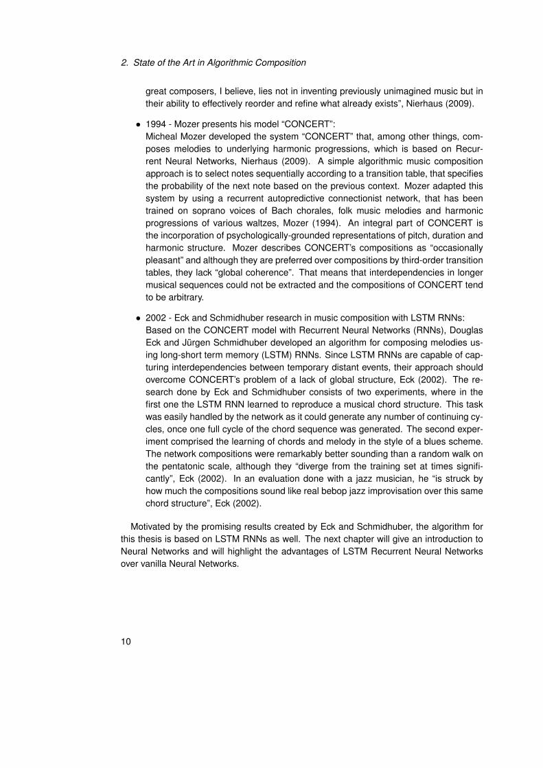
Neurons The “simple processing units” are called Neurons, which take a number of in-puts, sum all inputs together and compute the Neuron’s output by squashing the sum withan activation function.

Figure 3.1.: A Neuron. Source: Haykin (2004)

11

3. Neural Networks

The input signals xi , i = 1, 2, ..., m, are multiplied by a weight wki where k is refering tothe number of the current Neuron and i to the number of the input signal. The net input vk

is calculated by the sum over all input signals. Besides the inputs there is also a bias bk

feeding into the net input that gives the Neuron a tendency towards a specific behaviour.The net input vk can be calculated as follows:

uk =m∑

i=1

wkixi (3.1)

vk = uk + bk (3.2)

The net input vk can also be calculated with:

vk =m∑

i=0

wkixi (3.3)

where x0 = 1 and wk0 = bk .To calculate the output, also called activation, yk of a Neuron, an activation function ϕ(·)

is applied on the net input vk :

yk = ϕ(vk ) (3.4)

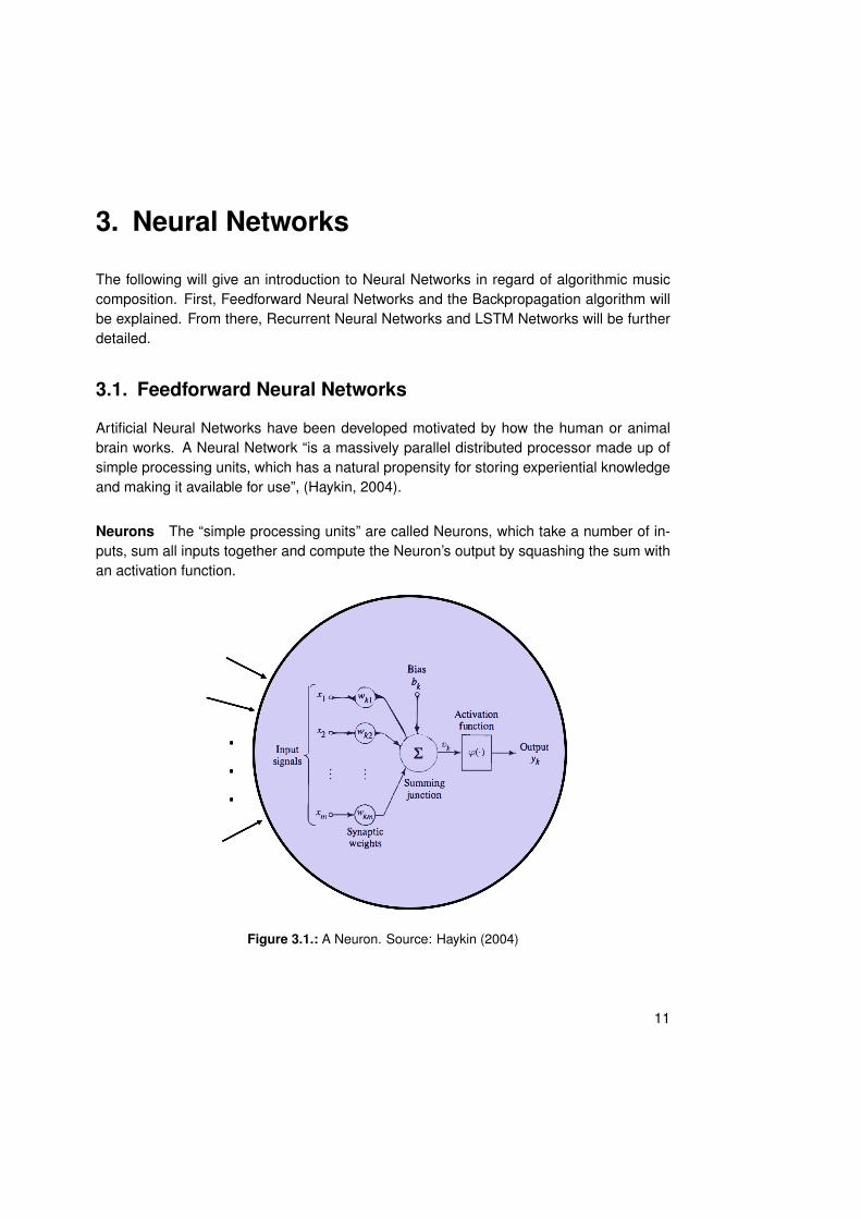
There are several types of activation functions used, while the sigmoid function is themost common one, which can be seen in equation 3.5. It squashes the net input to anoutput between 0 and 1.

σ(vk ) =1

1 + e(−a·vk ) (3.5)

Equation 3.5 shows the sigmoid function with a as the slope parameter. Figure 3.2 showsthe graph of the sigmoid function with different values for a.

Figure 3.2.: Sigmoid function with different values for the slope parameter. Source: Haykin (2004)

12

3.1. Feedforward Neural Networks

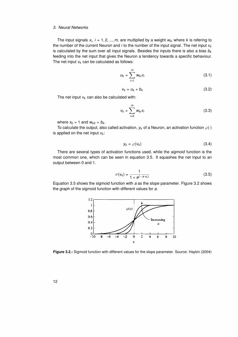
Network Architecture Making a Neural Network a “massively parallel distributed pro-cessor” is achieved by arranging and connecting several Neurons to a network with adistinct architecture. The simplest architecture is called a Single-layer Feedforward Net-work, Haykin (2004). It consists of two layers of Neurons, an input and an output layer.The Neurons between both layers are fully connected through “Synapses” with the synap-tic weight, Haykin (2004). Figure 3.3 shows a Single-layer Feedforward Network with fiveinput units and four Neurons as the output units. Every input unit feeds into each Neuronof the output layer.

Figure 3.3.: Single-layer Feedforward network with five input units and four Neurons as the output.Source: Johnson (2015)

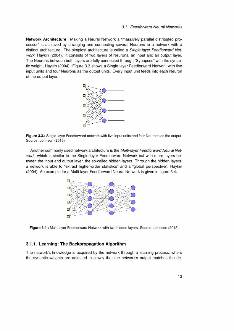
Another commonly used network architecture is the Multi-layer Feedforward Neural Net-work, which is similar to the Single-layer Feedforward Network but with more layers be-tween the input and output layer, the so-called hidden layers. Through the hidden layers,a network is able to “extract higher-order statistics” and a “global perspective”, Haykin(2004). An example for a Multi-layer Feedforward Neural Network is given in figure 3.4.

Figure 3.4.: Multi-layer Feedforward Network with two hidden layers. Source: Johnson (2015)

3.1.1. Learning: The Backpropagation Algorithm

The network’s knowledge is acquired by the network through a learning process, wherethe synaptic weights are adjusted in a way that the network’s output matches the de-

13

3. Neural Networks

sired output, which is called supervised learning. The network is trained with training data{(x (1), t (1)), (x (2), t (2)), ..., (x (n), t (n))}, consisting of input values x (n) and corresponding ex-pected target values t (n), where n is refering to the number of training samples.

Loss function By taking the difference of expected values (target values) tj and the net-work’s actual output yj when feeding it with the input training data, one gets a measure forthe networks performance. A commonly used loss function is the Squared Error functionin equation 3.6, where j refers to the j-th Neuron of the output layer and J refers to the totalnumber of Neurons in the output layer, Ng (2012b).

E(wki ) =12

∑j∈J

(yj − tj )2 (3.6)

Gradient Descent Learning takes place by adjusting the network’s synaptic weightswhile finding a minimum of the loss function. This is mostly done using the GradientDescent method, Rumelhart (1986). Equation 3.7 shows the update rule of gradient de-scent, where synaptic weights wki are usually initilized randomly at the beginning and areadjusted accordingly to equation 3.7, where α is the so-called learning rate, Ng (2012b).

wki := wki − α∂

∂wkiE(wki ) (3.7)

If the initilized values of wki are close enough to the optimum, and the learning rate α issmall enough, the gradient descent algorithm achieves linear convergence, Bottou (2010).

Computing Partial Derivatives To apply gradient descent as described in equation 3.7the partial derivatives of E(wki ) in regard of the weights wki must be computed. For this,two different cases will be treated where 1) the weights are connected between the lasthidden layer and the output layer and 2) the weights are connected between two hiddenlayers.

Weights at output layer For case 1) the following shows the computation of the partialderivative of E(wji ) in regard of the weights wji , Ng (2012a):

∂E∂wji

=∂

∂wji

12

∑j∈J

(yj − tj )2 (3.8)

∂E∂wji

= (yj − tj )∂

∂wjiyj (3.9)

Since the partial derivative of E is taken in regard of one specific wji , all terms of thesum except the one for the specific j will be zero. Applying chain rule onto the argument ofthe sum in equation 3.8 delivers equation 3.9. Since tj is constant the value of ∂tj

∂wjiis zero.

14

3.1. Feedforward Neural Networks

The output yj of the j-th Neuron in the output layer is equal to the net input of that Neuronsquashed by the activation function:

∂E∂wji

= (yj − tj )∂

∂wjiϕ(vj ) (3.10)

Applying chain rule onto ∂∂wji

ϕ(vj ) delivers:

∂E∂wji

= (yj − tj )ϕ′(vj )∂

∂wjivj (3.11)

The partial derivative of the net input vj in regard of the weight wji is simply the i-th inputxi of the Neuron.

∂E∂wji

= (yj − tj )ϕ′(vj )xi (3.12)

For reasons of simplicity we will define:

δj := (yj − tj )ϕ′(vj ) (3.13)

and get as a result for the partial derivative of E in regard of the weights wji from the lasthidden layer to the output layer:

∂E∂wji

= δjxi (3.14)

Weights between hidden layers From here on case 2) will be looked at, where theweight w (l)

ki is connected from the i-th Neuron in hidden layer l − 1 to the k -th Neuron inhidden layer l . In this case we cannot ommit the sum, as we did from equation 3.8 toequation 3.9 since the output yj of every Neuron in the output layer is dependent on allweights previous to the weights at the output layer.

∂E∂wki

=∂

∂wki

12

∑j∈J

(yj − tj )2 (3.15)

∂E∂wki

=∑j∈J

(yj − tj )∂

∂wkiyj (3.16)

Again applying yj = ϕ(vj ) and the chain rule delivers:

∂E∂wki

=∑j∈J

(yj − tj )∂

∂wkiϕ(vj ) (3.17)

∂E∂wki

=∑j∈J

(yj − tj )ϕ′(vj )∂

∂wkivj (3.18)

15

3. Neural Networks

∂E∂wki

=∑j∈J

(yj − tj )ϕ′(vj )∂vj

∂yk

∂yk

∂wki(3.19)

With ∂vj∂yk

= wjk and ∂yk∂wki

being independent of the sum we get:

∂E∂wki

=∂yk

∂wki

∑j∈J

(yj − tj )ϕ′(vj )wjk (3.20)

Applying yk = ϕ(vk ) and similar steps on ∂yk∂wki

as before we get:

∂E∂wki

= ϕ′(vk )∂vk

∂wki

∑j∈J

(yj − tj )ϕ′(vj )wjk (3.21)

∂E∂wki

= ϕ′(vk )xi

∑j∈J

(yj − tj )ϕ′(vj )wjk (3.22)

Using δj from equation 3.13 we get:

∂E∂wki

= xiϕ′(vk )

∑j∈J

δjwjk (3.23)

Again, for reasons of simplicity we will define:

δk := ϕ′(vk )∑j∈J

δjwjk (3.24)

And with that we get an expression for the partial derivative of E in regard of the weightswki between hidden layers:

∂E∂wki

= xiδk (3.25)

The Backpropagation algorithm With the equations 3.14 and 3.25 above we cannow formulate the Backpropagation learning algorithm on a fixed training data set{(x (1), t (1)), (x (2), t (2)), ..., (x (n), t (n))}, where x (n) is a vector of input values, t (n) is a vector oftarget values and n is the number of training samples, Ng (2012a).

1. For b = 1 to n:

a) Feed forward through the net with input values x (b)

b) For the output layer, compute δj

c) Backpropagate the error by computing δk for all layers previous to the outputlayer

16

3.2. Recurrent Neural Networks

d) Compute the partial derivatives for the output layer ∂E∂wji

= δjxi and for all hidden

layers ∂E∂wki

= xiδk .

e) Use gradient descent to update the weights wki := wki − α ∂∂wki

E(wki )

As we have seen, the network is learning to output the desired values by adjusting itsweights. Therefore the knowledge of a Neural Network is stored in the network’s weights,Haykin (2004). There are several methods available for training a Neural Network suchas adaptive step algorithms or second-order algorithms, Rojas (1996), while the abovedescribed Backpropagation algorithm is one of the most popular ones.

With the above described architecture of a Multi-layer Neural Network and an appropri-ate learning algorithm several tasks can be achieved, for example handwriting recognition,object recognition in image processing or spectroscopy in the field of chemistry, Svozil(1997). Although Multi-layer Neural Networks are achieving good results on those tasks,they lack the ability to capture patterns over time, which is key for music composition. Re-current Neural Networks are a special type of Neural Networks that can capture informationover time.

3.2. Recurrent Neural Networks

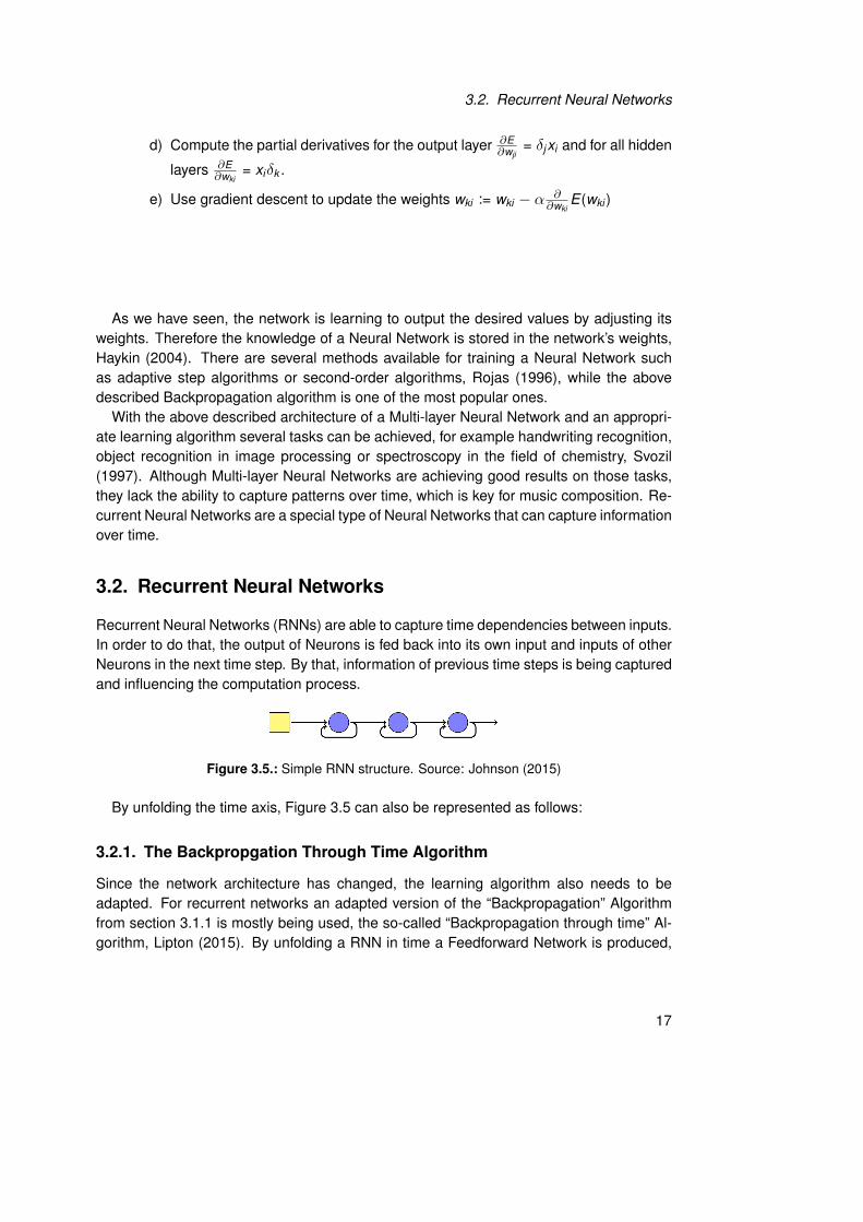
Recurrent Neural Networks (RNNs) are able to capture time dependencies between inputs.In order to do that, the output of Neurons is fed back into its own input and inputs of otherNeurons in the next time step. By that, information of previous time steps is being capturedand influencing the computation process.

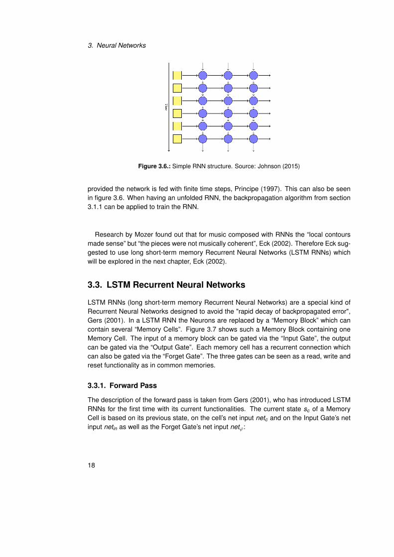
Figure 3.5.: Simple RNN structure. Source: Johnson (2015)

By unfolding the time axis, Figure 3.5 can also be represented as follows:

3.2.1. The Backpropgation Through Time Algorithm

Since the network architecture has changed, the learning algorithm also needs to beadapted. For recurrent networks an adapted version of the “Backpropagation” Algorithmfrom section 3.1.1 is mostly being used, the so-called “Backpropagation through time” Al-gorithm, Lipton (2015). By unfolding a RNN in time a Feedforward Network is produced,

17

3. Neural Networks

Figure 3.6.: Simple RNN structure. Source: Johnson (2015)

provided the network is fed with finite time steps, Principe (1997). This can also be seenin figure 3.6. When having an unfolded RNN, the backpropagation algorithm from section3.1.1 can be applied to train the RNN.

Research by Mozer found out that for music composed with RNNs the “local contoursmade sense” but “the pieces were not musically coherent”, Eck (2002). Therefore Eck sug-gested to use long short-term memory Recurrent Neural Networks (LSTM RNNs) whichwill be explored in the next chapter, Eck (2002).

3.3. LSTM Recurrent Neural Networks

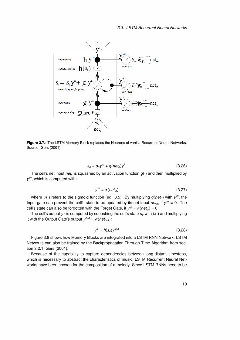
LSTM RNNs (long short-term memory Recurrent Neural Networks) are a special kind ofRecurrent Neural Networks designed to avoid the "rapid decay of backpropagated error",Gers (2001). In a LSTM RNN the Neurons are replaced by a “Memory Block” which cancontain several “Memory Cells”. Figure 3.7 shows such a Memory Block containing oneMemory Cell. The input of a memory block can be gated via the “Input Gate”, the outputcan be gated via the “Output Gate”. Each memory cell has a recurrent connection whichcan also be gated via the “Forget Gate”. The three gates can be seen as a read, write andreset functionality as in common memories.

3.3.1. Forward Pass

The description of the forward pass is taken from Gers (2001), who has introduced LSTMRNNs for the first time with its current functionalities. The current state sc of a MemoryCell is based on its previous state, on the cell’s net input netc and on the Input Gate’s netinput netin as well as the Forget Gate’s net input netϕ:

18

3.3. LSTM Recurrent Neural Networks

Figure 3.7.: The LSTM Memory Block replaces the Neurons of vanilla Recurrent Neural Networks.Source: Gers (2001)

sc = scyϕ + g(netc)y in (3.26)

The cell’s net input netc is squashed by an activation function g(·) and then multiplied byy in, which is computed with:

y in = σ(netin) (3.27)

where σ(·) refers to the sigmoid function (eq. 3.5). By multiplying g(netc) with y in, theInput gate can prevent the cell’s state to be updated by its net input netc , if y in = 0. Thecell’s state can also be forgotten with the Forget Gate, if yϕ = σ(netϕ) = 0.

The cell’s output yc is computed by squashing the cell’s state sc with h(·) and multiplyingit with the Output Gate’s output yout = σ(netout ):

yc = h(sc)yout (3.28)

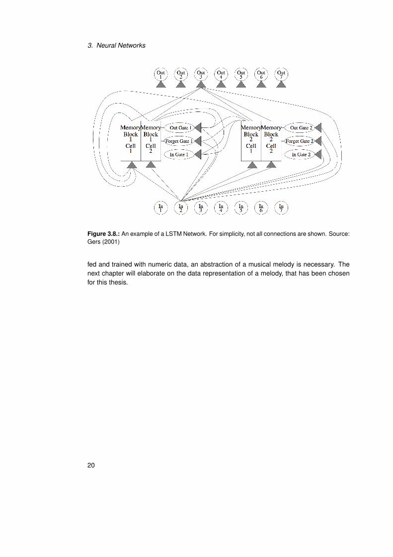
Figure 3.8 shows how Memory Blocks are integrated into a LSTM RNN Network. LSTMNetworks can also be trained by the Backpropagation Through Time Algorithm from sec-tion 3.2.1, Gers (2001).

Because of the capability to capture dependencies between long-distant timesteps,which is necessary to abstract the characteristics of music, LSTM Recurrent Neural Net-works have been chosen for the composition of a melody. Since LSTM RNNs need to be

19

3. Neural Networks

Figure 3.8.: An example of a LSTM Network. For simplicity, not all connections are shown. Source:Gers (2001)

fed and trained with numeric data, an abstraction of a musical melody is necessary. Thenext chapter will elaborate on the data representation of a melody, that has been chosenfor this thesis.

20

4. Data Representation: MIDI

In the previous chapter we have seen what Neural Networks are and that a LSTM RNNis the most promising type to use when it comes to music composition. For training andusing an LSTM RNN the question arises how music is going to be represented, in orderto make it accessible for the Neural Network. One possible option is to use vanilla audiodata, such as wave files, to feed the Neural Net. Another option is to use MIDI data, whichdoes not contain any audible sound, but information about the score of a musical piece.The next section will compare these two options and come to the conclusion to use MIDIdata for the implementation of the algorithm.

4.1. Comparison between Audio and MIDI

To decide whether Audio or MIDI data is the right choice to use, it is necessary to askfor the purpose of the Neural Network implementation. In this case, the purpose of theLSTM Network is to compose a melody or in other words find a melody to a given chordsequence. To reduce the complexity of this task, we are only interested in the pitch, thestart and the length of the melody’s notes. The velocity or other forms of articulation suchas bending will not be considered as part of this thesis.

Audio An audio signal is a very rich representation of music, since it can capture al-most every detail of music, depending on the audio format and quality. For example, audiosignals contain the timbre of instruments, which is the characteristic spectrum of an instru-ment, its characertistic transients as well as the development of the spectrum over time,Levitin (2006). To reduce the complexity of an audio signal to just the pitch, the start andthe length of the notes in a melody, rather complex methods have to applied. For example,to extract the pitch of a note a Fourier Transform is necessary to detect the base frequencyof this tone which then need to be mapped to a specific pitch, which also is a nonlinearfunction, Zwicker (1999). To extract the start of a note the transients would have to bedetected with a Beat Detection algorithm and then need to be mapped to a timestep ofthe network. This shows that it is a rather complex undertaking to extract the necessaryfeatures for the Neural Network model used in this thesis.

MIDI MIDI (Musical Instrument Digital Interface) is a standardized data protocol to ex-change musical control data between digital intruments. Nowadays it is mostly being used

21

4. Data Representation: MIDI

in the context of computer music, where the actual sound is created by instruments or syn-thesizers in the computer. MIDI data is fed into a synthesizer with the information abouta note’s start, duration, and pitch. In addition there are several other options to control adigital instrument with MIDI data, which are not relevant for this thesis. MIDI data alreadycontains the necessary information needed to feed the Neural Network and it only needs tobe transformed into an appropriate numeric representation for the LSTM RNN. Thus, MIDIdata has been chosen to represent music on a very basic level: pitch, start and lengthof notes. The following chapter elaborates how MIDI data will be transformed to make itaccessible for the Neural Network.

4.2. Piano Roll Representation

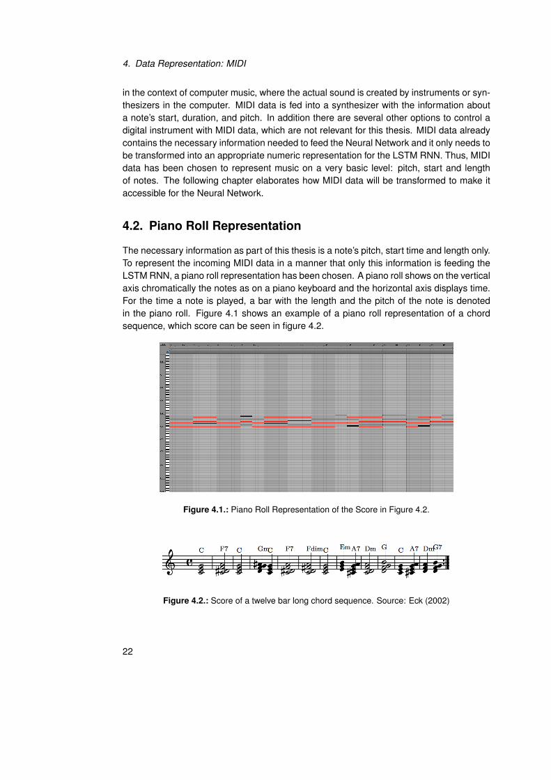
The necessary information as part of this thesis is a note’s pitch, start time and length only.To represent the incoming MIDI data in a manner that only this information is feeding theLSTM RNN, a piano roll representation has been chosen. A piano roll shows on the verticalaxis chromatically the notes as on a piano keyboard and the horizontal axis displays time.For the time a note is played, a bar with the length and the pitch of the note is denotedin the piano roll. Figure 4.1 shows an example of a piano roll representation of a chordsequence, which score can be seen in figure 4.2.

Figure 4.1.: Piano Roll Representation of the Score in Figure 4.2.

Figure 4.2.: Score of a twelve bar long chord sequence. Source: Eck (2002)

22

4.2. Piano Roll Representation

The piano roll representation is transformed to a two-dimensional matrix with pitch asthe first dimension and time as the second dimension. Time is quantized in MIDI ticks,where the default setting is 96 ticks per beat and one beat typically refers to a quarter notewik (2015). 96 ticks per beat lead to a resolution of a 1

384 -th note per timestep, which is farto granular for the purposes of this thesis, since the melodies used for this thesis containno shorter notes than 1

16 -th notes. To reduce the computation costs, the number of ticksper beat needs to be reduced. 4 ticks per beat lead to a resolution of a 1

16 -th note pertimestep and the number of 1

16 -th quantization steps in a MIDI file determines thereforethe size of the time axis. The size of the pitch axis is dependent on the note range of apiece. All pitches below the lowest note and all pitches higher than the highest note will beneglected. Therefore, the piano roll matrix is of the size (num of 1

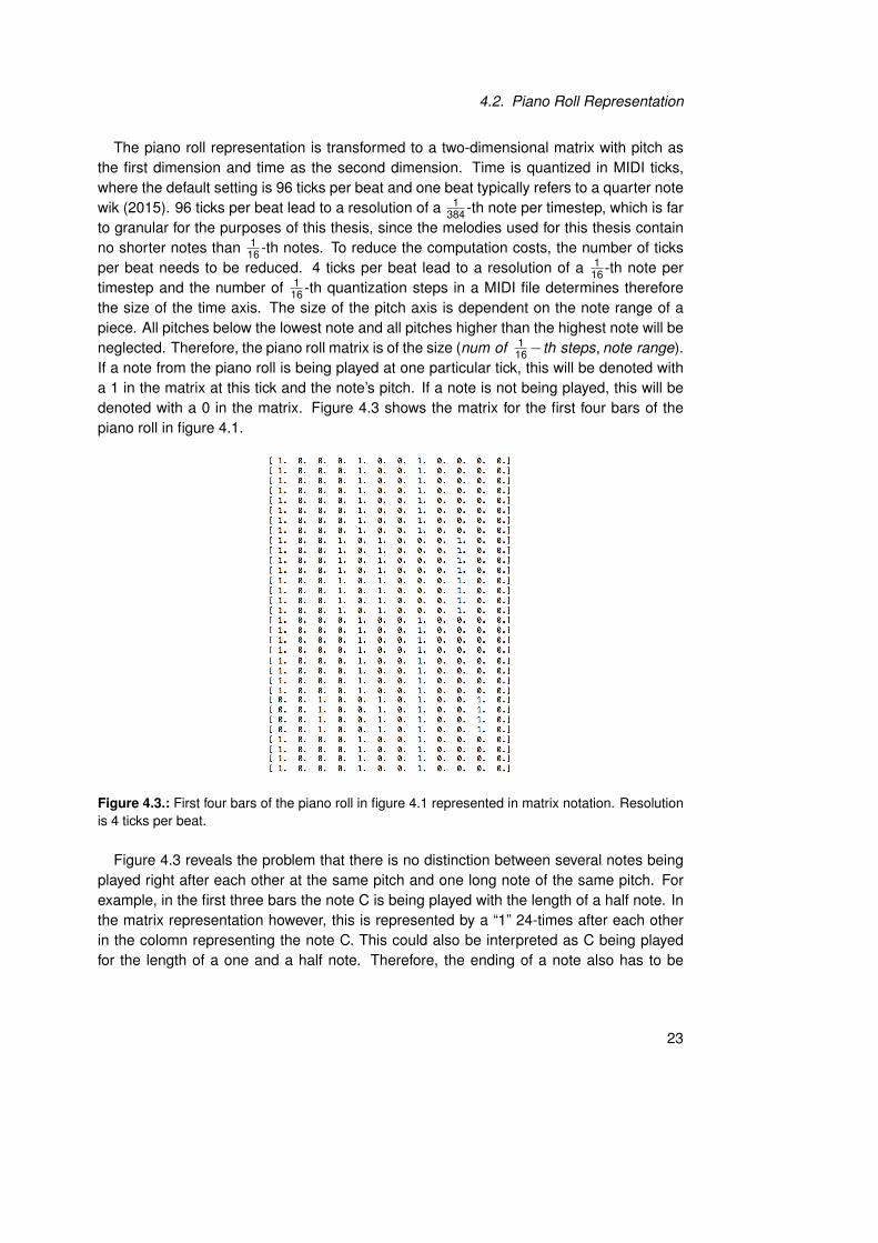
16−th steps, note range).If a note from the piano roll is being played at one particular tick, this will be denoted witha 1 in the matrix at this tick and the note’s pitch. If a note is not being played, this will bedenoted with a 0 in the matrix. Figure 4.3 shows the matrix for the first four bars of thepiano roll in figure 4.1.

Figure 4.3.: First four bars of the piano roll in figure 4.1 represented in matrix notation. Resolutionis 4 ticks per beat.

Figure 4.3 reveals the problem that there is no distinction between several notes beingplayed right after each other at the same pitch and one long note of the same pitch. Forexample, in the first three bars the note C is being played with the length of a half note. Inthe matrix representation however, this is represented by a “1” 24-times after each otherin the colomn representing the note C. This could also be interpreted as C being playedfor the length of a one and a half note. Therefore, the ending of a note also has to be

23

4. Data Representation: MIDI

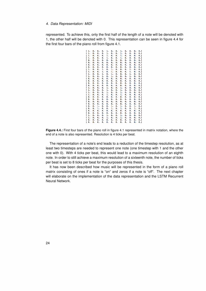
represented. To achieve this, only the first half of the length of a note will be denoted with1, the other half will be denoted with 0. This representation can be seen in figure 4.4 forthe first four bars of the piano roll from figure 4.1.

Figure 4.4.: First four bars of the piano roll in figure 4.1 represented in matrix notation, where theend of a note is also represented. Resolution is 4 ticks per beat.

The representation of a note’s end leads to a reduction of the timestep resolution, as atleast two timesteps are needed to represent one note (one timestep with 1 and the otherone with 0). With 4 ticks per beat, this would lead to a maximum resolution of an eighthnote. In order to still achieve a maximum resolution of a sixteenth note, the number of ticksper beat is set to 8 ticks per beat for the purposes of this thesis.

It has now been described how music will be represented in the form of a piano rollmatrix consisting of ones if a note is “on“ and zeros if a note is “off“. The next chapterwill elaborate on the implementation of the data representation and the LSTM RecurrentNeural Network.

24

5. Implementation

For reasons of fast implementation the programming language “Python” has been chosen,since there exist several Neural Network and MIDI libraries for Python. For implementingthe LSTM RNN the library “Keras” has been chosen, which is a library built on “Theano”.Theano is another python library that allows for fast optimization and evaluation of math-ematical expressions, which is often used in Neural Network applications. While Theanoallows for higher modularity and customization of a Neural Network implementation, it isalso more complex, thus involves a steeper learning curve. At the same time, Keras isless modular and comes along with a few constraints, but allows the user to implement aNeural Network very easily and quickly. Therefore, due to time constraints of this thesis,Keras has been chosen as the framework for implementing the LSTM RNN.

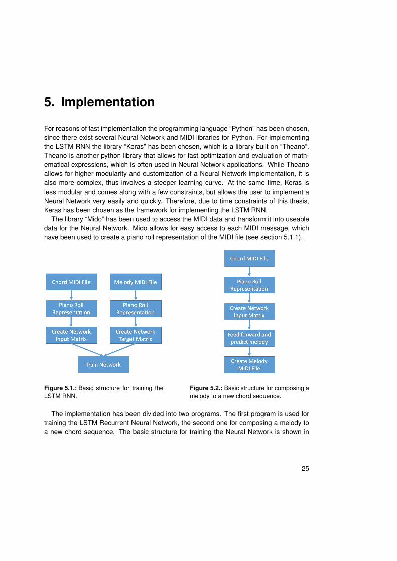
The library “Mido” has been used to access the MIDI data and transform it into useabledata for the Neural Network. Mido allows for easy access to each MIDI message, whichhave been used to create a piano roll representation of the MIDI file (see section 5.1.1).

Figure 5.1.: Basic structure for training theLSTM RNN.

Figure 5.2.: Basic structure for composing amelody to a new chord sequence.

The implementation has been divided into two programs. The first program is used fortraining the LSTM Recurrent Neural Network, the second one for composing a melody toa new chord sequence. The basic structure for training the Neural Network is shown in

25

5. Implementation

figure 5.1 and for composing a melody in figure 5.2. The following will elaborate on theimplementation of the training program as well as of the composition program.

5.1. The Training Program

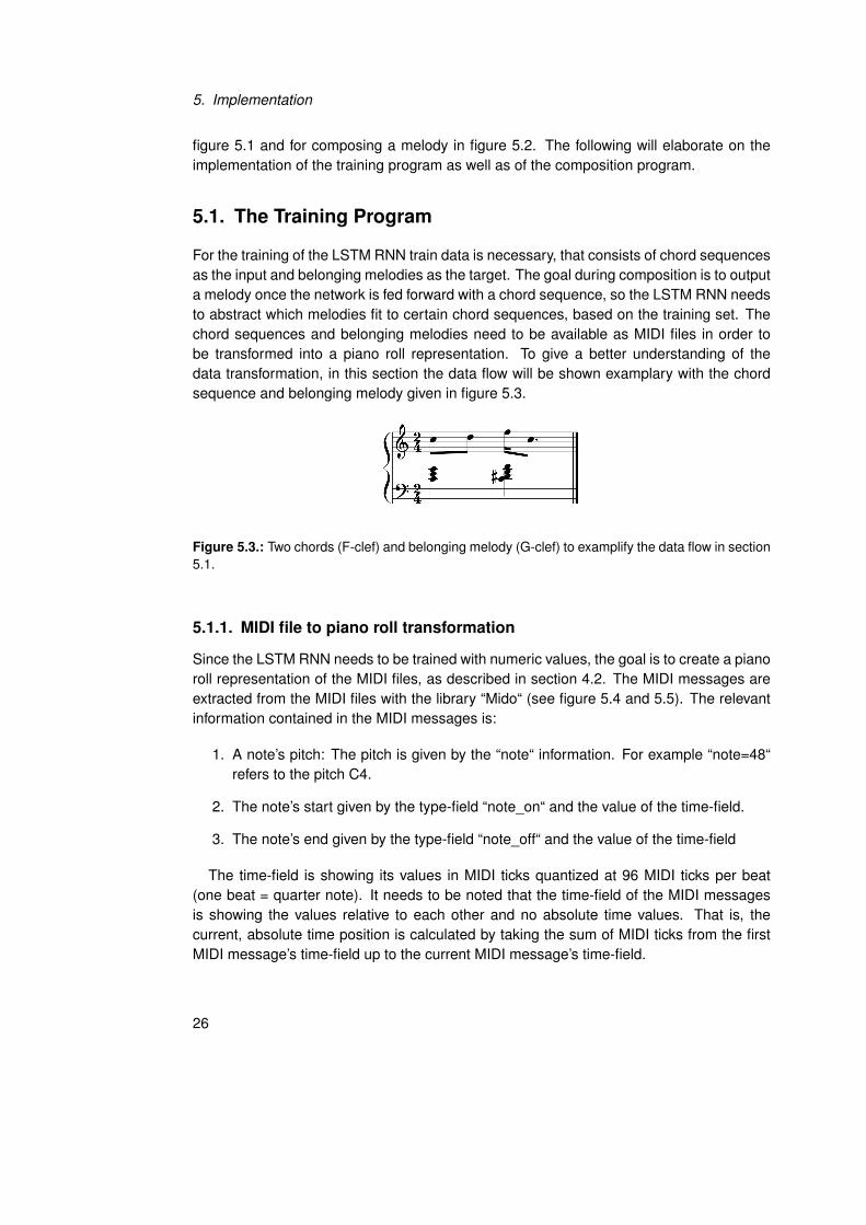
For the training of the LSTM RNN train data is necessary, that consists of chord sequencesas the input and belonging melodies as the target. The goal during composition is to outputa melody once the network is fed forward with a chord sequence, so the LSTM RNN needsto abstract which melodies fit to certain chord sequences, based on the training set. Thechord sequences and belonging melodies need to be available as MIDI files in order tobe transformed into a piano roll representation. To give a better understanding of thedata transformation, in this section the data flow will be shown examplary with the chordsequence and belonging melody given in figure 5.3.

Figure 5.3.: Two chords (F-clef) and belonging melody (G-clef) to examplify the data flow in section5.1.

5.1.1. MIDI file to piano roll transformation

Since the LSTM RNN needs to be trained with numeric values, the goal is to create a pianoroll representation of the MIDI files, as described in section 4.2. The MIDI messages areextracted from the MIDI files with the library “Mido“ (see figure 5.4 and 5.5). The relevantinformation contained in the MIDI messages is:

1. A note’s pitch: The pitch is given by the “note“ information. For example “note=48“refers to the pitch C4.

2. The note’s start given by the type-field “note_on“ and the value of the time-field.

3. The note’s end given by the type-field “note_off“ and the value of the time-field

The time-field is showing its values in MIDI ticks quantized at 96 MIDI ticks per beat(one beat = quarter note). It needs to be noted that the time-field of the MIDI messagesis showing the values relative to each other and no absolute time values. That is, thecurrent, absolute time position is calculated by taking the sum of MIDI ticks from the firstMIDI message’s time-field up to the current MIDI message’s time-field.

26

5.1. The Training Program

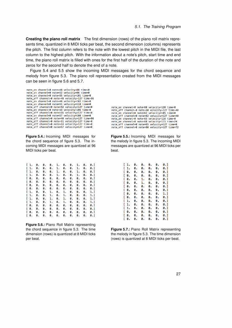
Creating the piano roll matrix The first dimension (rows) of the piano roll matrix repre-sents time, quantized in 8 MIDI ticks per beat, the second dimension (columns) representsthe pitch. The first column refers to the note with the lowest pitch in the MIDI file, the lastcolumn to the highest pitch. With the information about a note’s pitch, start time and endtime, the piano roll matrix is filled with ones for the first half of the duration of the note andzeros for the second half to denote the end of a note.

Figure 5.4 and 5.5 show the incoming MIDI messages for the chord sequence andmelody from figure 5.3. The piano roll representation created from the MIDI messagescan be seen in figure 5.6 and 5.7.

Figure 5.4.: Incoming MIDI messages forthe chord sequence of figure 5.3. The in-coming MIDI messages are quantized at 96MIDI ticks per beat.

Figure 5.5.: Incoming MIDI messages forthe melody in figure 5.3. The incoming MIDImessages are quantized at 96 MIDI ticks perbeat.

Figure 5.6.: Piano Roll Matrix representingthe chord sequence in figure 5.3. The timedimension (rows) is quantized at 8 MIDI ticksper beat.

Figure 5.7.: Piano Roll Matrix representingthe melody in figure 5.3. The time dimension(rows) is quantized at 8 MIDI ticks per beat.

27

5. Implementation

5.1.2. Network Inputs and Targets

So far it has been shown how the transformation from a MIDI file to a piano roll represen-tation has been implemented. However, in order to make the data useable for the Kerasframework, the piano roll representations need to be transformed into a Network Input Ma-trix and a Prediction Target Matrix. Both matrices consist of training samples, where in thecase of the Network Input Matrix one network input sample consists of a 2-dimensionalinput matrix and in the case of the Prediction Target Matrix one target sample consists ofa 1-dimensional target vector.

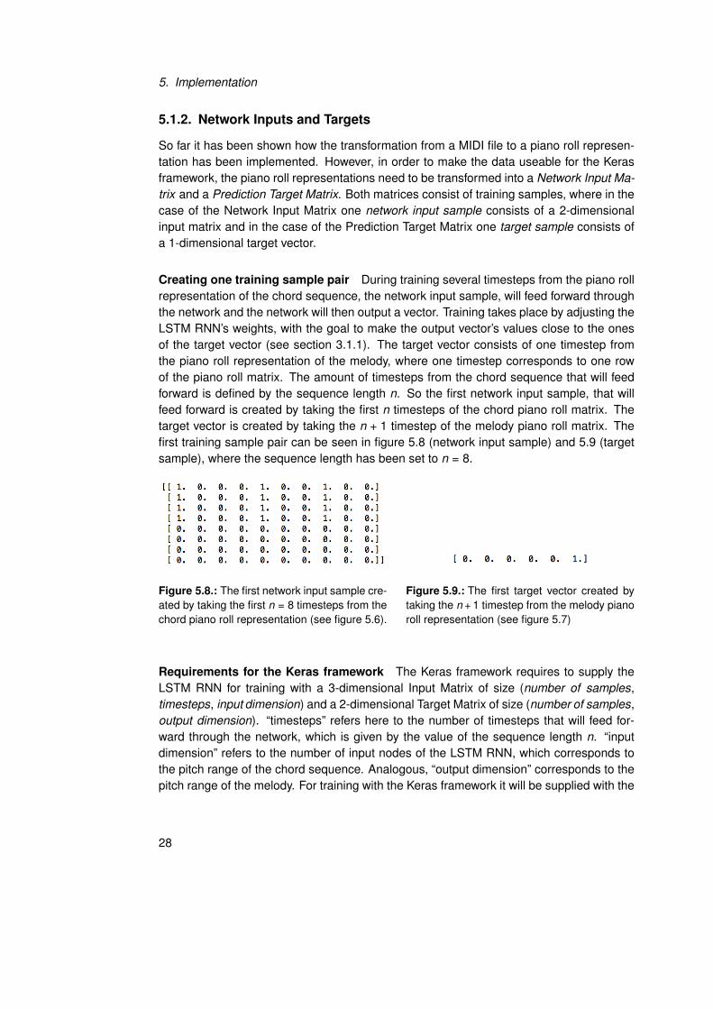
Creating one training sample pair During training several timesteps from the piano rollrepresentation of the chord sequence, the network input sample, will feed forward throughthe network and the network will then output a vector. Training takes place by adjusting theLSTM RNN’s weights, with the goal to make the output vector’s values close to the onesof the target vector (see section 3.1.1). The target vector consists of one timestep fromthe piano roll representation of the melody, where one timestep corresponds to one rowof the piano roll matrix. The amount of timesteps from the chord sequence that will feedforward is defined by the sequence length n. So the first network input sample, that willfeed forward is created by taking the first n timesteps of the chord piano roll matrix. Thetarget vector is created by taking the n + 1 timestep of the melody piano roll matrix. Thefirst training sample pair can be seen in figure 5.8 (network input sample) and 5.9 (targetsample), where the sequence length has been set to n = 8.

Figure 5.8.: The first network input sample cre-ated by taking the first n = 8 timesteps from thechord piano roll representation (see figure 5.6).

Figure 5.9.: The first target vector created bytaking the n + 1 timestep from the melody pianoroll representation (see figure 5.7)

Requirements for the Keras framework The Keras framework requires to supply theLSTM RNN for training with a 3-dimensional Input Matrix of size (number of samples,timesteps, input dimension) and a 2-dimensional Target Matrix of size (number of samples,output dimension). “timesteps” refers here to the number of timesteps that will feed for-ward through the network, which is given by the value of the sequence length n. “inputdimension” refers to the number of input nodes of the LSTM RNN, which corresponds tothe pitch range of the chord sequence. Analogous, “output dimension” corresponds to thepitch range of the melody. For training with the Keras framework it will be supplied with the

28

5.1. The Training Program

Network Input Matrix of size (number of samples, sequencelengthn, chord pitchrange) andthe Prediction Target Matrix of size (number of samples, melody pitch range). The num-ber of samples is given by the difference between the number of timesteps of the pianoroll matrix and the sequence length: number of samples = number of timestepspiano roll −sequence length.

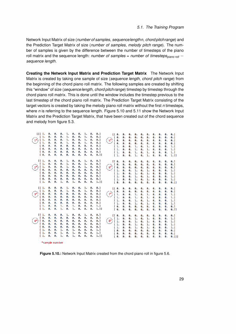
Creating the Network Input Matrix and Prediction Target Matrix The Network InputMatrix is created by taking one sample of size (sequence length, chord pitch range) fromthe beginning of the chord piano roll matrix. The following samples are created by shiftingthis “window” of size (sequence length, chord pitchrange) timestep by timestep through thechord piano roll matrix. This is done until the window includes the timestep previous to thelast timestep of the chord piano roll matrix. The Prediction Target Matrix consisting of thetarget vectors is created by taking the melody piano roll matrix without the first n timesteps,where n is referring to the sequence length. Figure 5.10 and 5.11 show the Network InputMatrix and the Prediction Target Matrix, that have been created out of the chord sequenceand melody from figure 5.3.

Figure 5.10.: Network Input Matrix created from the chord piano roll in figure 5.6.

29

5. Implementation

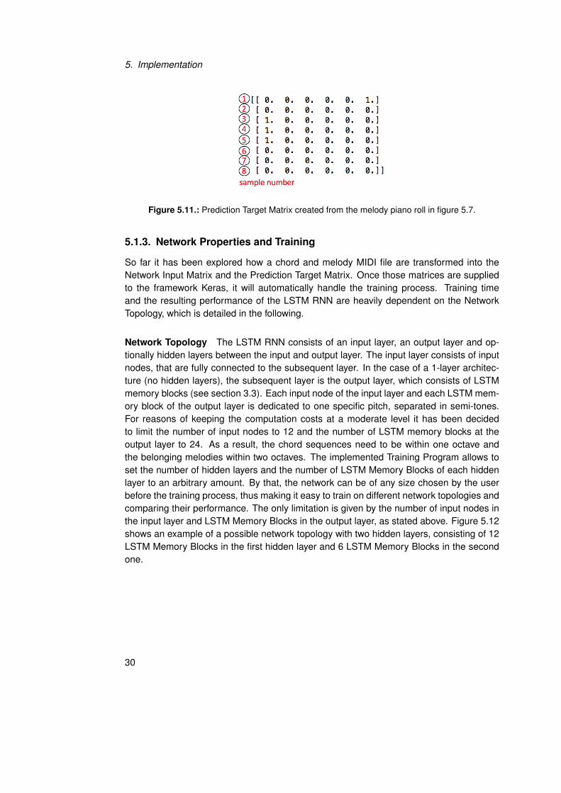
Figure 5.11.: Prediction Target Matrix created from the melody piano roll in figure 5.7.

5.1.3. Network Properties and Training

So far it has been explored how a chord and melody MIDI file are transformed into theNetwork Input Matrix and the Prediction Target Matrix. Once those matrices are suppliedto the framework Keras, it will automatically handle the training process. Training timeand the resulting performance of the LSTM RNN are heavily dependent on the NetworkTopology, which is detailed in the following.

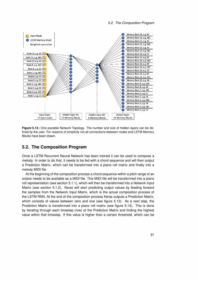
Network Topology The LSTM RNN consists of an input layer, an output layer and op-tionally hidden layers between the input and output layer. The input layer consists of inputnodes, that are fully connected to the subsequent layer. In the case of a 1-layer architec-ture (no hidden layers), the subsequent layer is the output layer, which consists of LSTMmemory blocks (see section 3.3). Each input node of the input layer and each LSTM mem-ory block of the output layer is dedicated to one specific pitch, separated in semi-tones.For reasons of keeping the computation costs at a moderate level it has been decidedto limit the number of input nodes to 12 and the number of LSTM memory blocks at theoutput layer to 24. As a result, the chord sequences need to be within one octave andthe belonging melodies within two octaves. The implemented Training Program allows toset the number of hidden layers and the number of LSTM Memory Blocks of each hiddenlayer to an arbitrary amount. By that, the network can be of any size chosen by the userbefore the training process, thus making it easy to train on different network topologies andcomparing their performance. The only limitation is given by the number of input nodes inthe input layer and LSTM Memory Blocks in the output layer, as stated above. Figure 5.12shows an example of a possible network topology with two hidden layers, consisting of 12LSTM Memory Blocks in the first hidden layer and 6 LSTM Memory Blocks in the secondone.

30

5.2. The Composition Program

Figure 5.12.: One possible Network Topology. The number and size of hidden layers can be de-fined by the user. For reasons of simplicity not all connections between nodes and LSTM MemoryBlocks have been drawn.

5.2. The Composition Program

Once a LSTM Recurrent Neural Network has been trained it can be used to compose amelody. In order to do that, it needs to be fed with a chord sequence and will then outputa Prediction Matrix, which can be transformed into a piano roll matrix and finally into amelody MIDI file.

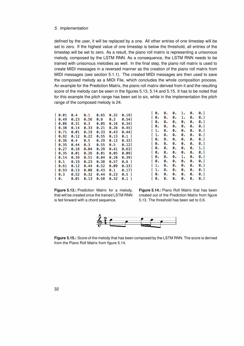
At the beginning of the composition process a chord sequence within a pitch range of anoctave needs to be available as a MIDI file. This MIDI file will be transformed into a pianoroll representation (see section 5.1.1), which will then be transformed into a Network InputMatrix (see section 5.1.2). Keras will start predicting output values by feeding forwardthe samples from the Network Input Matrix, which is the actual composition process ofthe LSTM RNN. At the end of the composition process Keras outputs a Prediction Matrix,which consists of values between zero and one (see figure 5.13). As a next step, thePrediction Matrix is transformed into a piano roll matrix (see figure 5.14). This is doneby iterating through each timestep (row) of the Prediction Matrix and finding the highestvalue within that timestep. If this value is higher than a certain threshold, which can be

31

5. Implementation

defined by the user, it will be replaced by a one. All other entries of one timestep will beset to zero. If the highest value of one timestep is below the threshold, all entries of thetimestep will be set to zero. As a result, the piano roll matrix is representing a unisonousmelody, composed by the LSTM RNN. As a consequence, the LSTM RNN needs to betrained with unisonous melodies as well. In the final step, the piano roll matrix is used tocreate MIDI messages in a reversed manner as the creation of the piano roll matrix fromMIDI messages (see section 5.1.1). The created MIDI messages are then used to savethe composed melody as a MIDI File, which concludes the whole composition process.An example for the Prediction Matrix, the piano roll matrix derived from it and the resultingscore of the melody can be seen in the figures 5.13, 5.14 and 5.15. It has to be noted thatfor this example the pitch range has been set to six, while in the implementation the pitchrange of the composed melody is 24.

Figure 5.13.: Prediction Matrix for a melody,that will be created once the trained LSTM RNNis fed forward with a chord sequence.

Figure 5.14.: Piano Roll Matrix that has beencreated out of the Prediction Matrix from figure5.13. The threshold has been set to 0.6.

Figure 5.15.: Score of the melody that has been composed by the LSTM RNN. The score is derivedfrom the Piano Roll Matrix from figure 5.14.

32

6. Experiments

In section 5 the implementation of the LSTM Melody Composer has been described. Thefollowing will detail the experiments, that have been done with the Training and Compo-sition Program. First, the train and test data will be described, that is the chords andmelodies that have been used to train the LSTM RNN and the chords, that have been usedfor composing a melody. The train data has been used to train on eleven different networktopologies. This procedure will be described in section 6.2 as well as the melodies thathave been composed by the different networks. Finally, a decision on one network topol-ogy has been made that composes the most promising melodies for evaluating the qualityof the compositions, which will be further explained in chapter 7.

6.1. Train and Test Data

The selection for the train data is a crucial part of the quality of the LSTM RNN’s compo-sitions. The LSTM RNN is deriving its “knowledge” about music from the train data only,so the better the train data, the better the LSTM RNN will perform. Also, a compositionalgoal needs to be defined in order to make a decision on the train data. For example, if thegoal is to compose atonal melodies, the train data must consist of atonal melodies only.The test data should usually be different from the train data in order to see whether theLSTM RNN was able to make an abstraction of the train data and compose new melodiesinstead of simply creating a reproduction of the train data. The train and test data for thepurposes of this thesis will be described in the following.

Train Data There are two compositional goals for the LSTM RNN. First, the LSTM RNNshould compose melodies that cannot be recognized as computer compositions and there-fore cannot be distiguished from melodies composed by humans. Second, the melodiesshould simply sound pleasantly to the listener. While the first goal requires to use melodiesthat have been composed by humans, it is not easy to derive a requirement for the testdata from the second goal. The composed melodies should sound pleasant to the listener,but people have different tastes in music. A melody could sound very pleasant to onelistener, but displeasing to another one. Therefore a decision for the train data has beenmade based on music that is appealing to a large group of people, namely songs from“The Beatles”. Since The Beatles have been one of the most successful bands in historyand their music is still influencing the creations of several musicians from today, creating

33

6. Experiments

the train data from Beatles songs seems to be a good representation for music that soundspleasantly to a large group of people.

Another requirement is to compose melodies of a rather short duration, in order to makethem usable for the listening test in the evaluation part. Although the LSTM RNN is able tocompose melodies of any length, the melodies for the evaluation should be of a length of8 bars. Therefore, the chords and melodies in the train data have been set to a length of 8bars.

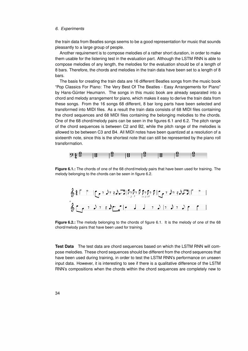
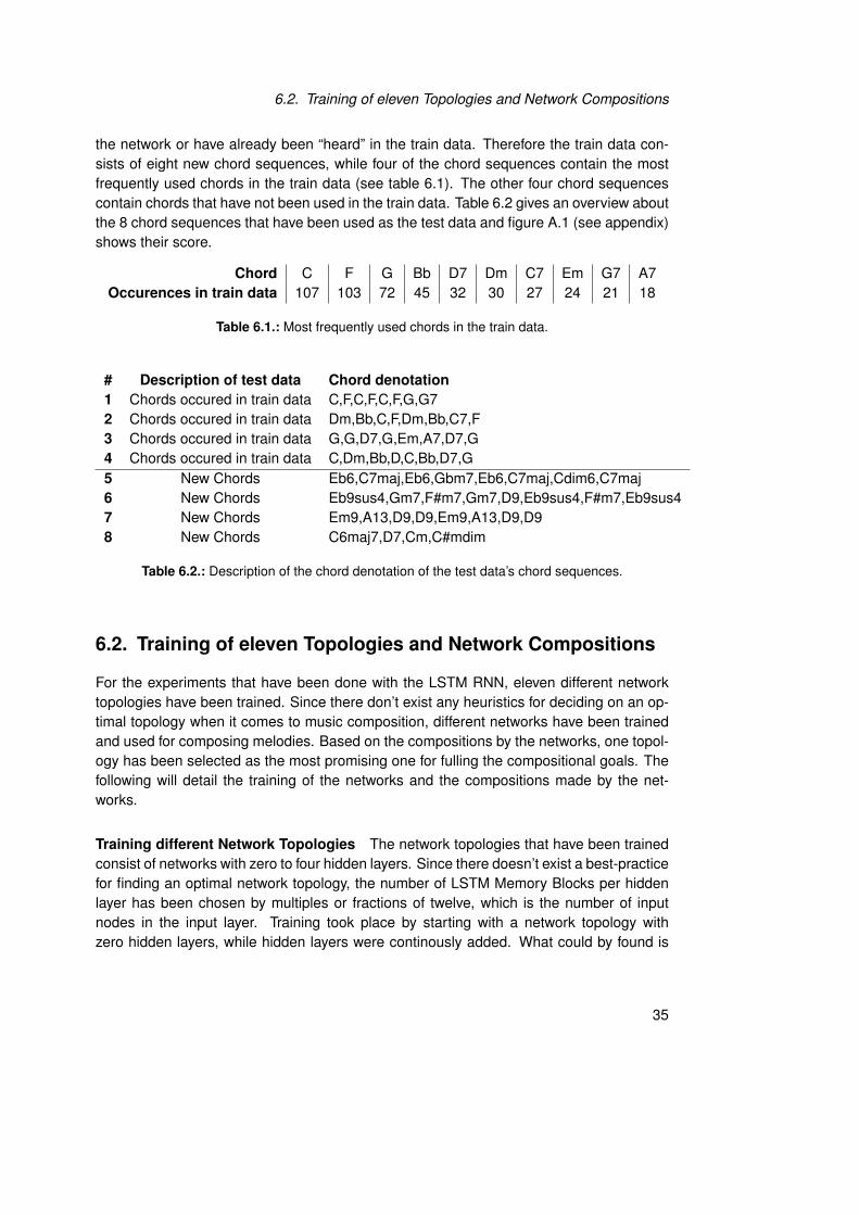
The basis for creating the train data are 16 different Beatles songs from the music book“Pop Classics For Piano: The Very Best Of The Beatles - Easy Arrangements for Piano”by Hans-Günter Heumann. The songs in this music book are already separated into achord and melody arrangement for piano, which makes it easy to derive the train data fromthese songs. From the 16 songs 68 different, 8 bar long parts have been selected andtransformed into MIDI files. As a result the train data consists of 68 MIDI files containingthe chord sequences and 68 MIDI files containing the belonging melodies to the chords.One of the 68 chord/melody pairs can be seen in the figures 6.1 and 6.2. The pitch rangeof the chord sequences is between C2 and B2, while the pitch range of the melodies isallowed to be between C3 and B4. All MIDI notes have been quantized at a resolution of asixteenth note, since this is the shortest note that can still be represented by the piano rolltransformation.

Figure 6.1.: The chords of one of the 68 chord/melody pairs that have been used for training. Themelody belonging to the chords can be seen in figure 6.2.

Figure 6.2.: The melody belonging to the chords of figure 6.1. It is the melody of one of the 68chord/melody pairs that have been used for training.

Test Data The test data are chord sequences based on which the LSTM RNN will com-pose melodies. These chord sequences should be different from the chord sequences thathave been used during training, in order to test the LSTM RNN’s performance on unseeninput data. However, it is interesting to see if there is a qualitative difference of the LSTMRNN’s compositions when the chords within the chord sequences are completely new to

34

6.2. Training of eleven Topologies and Network Compositions

the network or have already been “heard” in the train data. Therefore the train data con-sists of eight new chord sequences, while four of the chord sequences contain the mostfrequently used chords in the train data (see table 6.1). The other four chord sequencescontain chords that have not been used in the train data. Table 6.2 gives an overview aboutthe 8 chord sequences that have been used as the test data and figure A.1 (see appendix)shows their score.

Chord C F G Bb D7 Dm C7 Em G7 A7Occurences in train data 107 103 72 45 32 30 27 24 21 18

Table 6.1.: Most frequently used chords in the train data.

# Description of test data Chord denotation1 Chords occured in train data C,F,C,F,C,F,G,G72 Chords occured in train data Dm,Bb,C,F,Dm,Bb,C7,F3 Chords occured in train data G,G,D7,G,Em,A7,D7,G4 Chords occured in train data C,Dm,Bb,D,C,Bb,D7,G5 New Chords Eb6,C7maj,Eb6,Gbm7,Eb6,C7maj,Cdim6,C7maj6 New Chords Eb9sus4,Gm7,F#m7,Gm7,D9,Eb9sus4,F#m7,Eb9sus47 New Chords Em9,A13,D9,D9,Em9,A13,D9,D98 New Chords C6maj7,D7,Cm,C#mdim

Table 6.2.: Description of the chord denotation of the test data’s chord sequences.

6.2. Training of eleven Topologies and Network Compositions

For the experiments that have been done with the LSTM RNN, eleven different networktopologies have been trained. Since there don’t exist any heuristics for deciding on an op-timal topology when it comes to music composition, different networks have been trainedand used for composing melodies. Based on the compositions by the networks, one topol-ogy has been selected as the most promising one for fulling the compositional goals. Thefollowing will detail the training of the networks and the compositions made by the net-works.

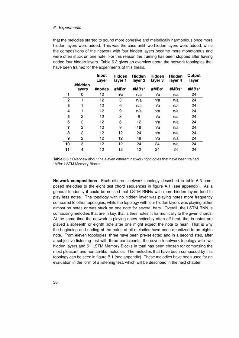
Training different Network Topologies The network topologies that have been trainedconsist of networks with zero to four hidden layers. Since there doesn’t exist a best-practicefor finding an optimal network topology, the number of LSTM Memory Blocks per hiddenlayer has been chosen by multiples or fractions of twelve, which is the number of inputnodes in the input layer. Training took place by starting with a network topology withzero hidden layers, while hidden layers were continously added. What could by found is

35

6. Experiments

that the melodies started to sound more cohesive and melodically harmonious once morehidden layers were added. This was the case until two hidden layers were added, whilethe compositions of the network with four hidden layers became more monotonous andwere often stuck on one note. For this reason the training has been stopped after havingadded four hidden layers. Table 6.3 gives an overview about the network topologies thathave been trained for the experiments of this thesis.

InputLayer

Hiddenlayer 1

Hiddenlayer 2

Hiddenlayer 3

Hiddenlayer 4

Outputlayer

#hiddenlayers #nodes #MBs* #MBs* #MBs* #MBs* #MBs*

1 0 12 n/a n/a n/a n/a 242 1 12 3 n/a n/a n/a 243 1 12 6 n/a n/a n/a 244 1 12 9 n/a n/a n/a 245 2 12 3 6 n/a n/a 246 2 12 6 12 n/a n/a 247 2 12 9 18 n/a n/a 248 2 12 12 24 n/a n/a 249 2 12 12 48 n/a n/a 24

10 3 12 12 24 24 n/a 2411 4 12 12 12 24 24 24

Table 6.3.: Overview about the eleven different network topologies that have been trained.*MBs: LSTM Memory Blocks

Network compositions Each different network topology described in table 6.3 com-posed melodies to the eight test chord sequences in figure A.1 (see appendix). As ageneral tendency it could be noticed that LSTM RNNs with more hidden layers tend toplay less notes. The topology with no hidden layer was playing notes more frequentlycompared to other topologies, while the topology with four hidden layers was playing eitheralmost no notes or was stuck on one note for several bars. Overall, the LSTM RNN iscomposing melodies that are in key, that is their notes fit harmonically to the given chords.At the same time the network is playing notes noticably often off beat, that is notes areplayed a sixteenth or eighth note after one might expect the note to hear. That is whythe beginning and ending of the notes of all melodies have been quantized to an eighthnote. From eleven topologies, three have been pre-selected and in a second step, aftera subjective listening test with three participants, the seventh network topology with twohidden layers and 51 LSTM Memory Blocks in total has been chosen for composing themost pleasant and human-like melodies. The melodies that have been composed by thistopology can be seen in figure B.1 (see appendix). These melodies have been used for anevaluation in the form of a listening test, which will be described in the next chapter.

36

7. Evaluation

The previous chapters have explained how the LSTM Recurrent Neural Network has beenimplemented and the experiments that have been done with the implementation. Thischapter will elaborate on the evaluation of the composed melodies in order to assess thequality of the LSTM RNN’s compositions. The evaluation has been desgined influenced bya framework described in the paper “Towards A Framework for the Evaluation of MachineCompositions”, Pearce. The framework is comprised of the following steps:

1. Specifying the compositional aims

2. Inducing a critic from a set of example musical phrases

3. Composing music that satisfies the critic

4. Evaluating specific claims about the compositions in experiments using human sub-jects

While the compositional aims have already been described, the involvement of a criticis done by creating human compositions as a comparison for the computer compositions.The main focus of the following is the evaluation in experiements using human subjects.

7.1. Subjective Listening Test

Due to the nature of the task for this thesis, direct objective measures cannot be applied,since “the evaluation of beauty or aesthetic value in works of art (including music) oftencomes down to individual subjective opinion”, Pearce. Therefore a listening test with hu-man subjects has been designed in order to evaluate the compositional goals for the LSTMRNN:

1. Compose melodies that cannot be distinguished from human melodies.

2. The melodies should sound pleasantly to the listener.

7.1.1. Test Design

Derived from the compositional goals above, the listening test has been seperated into twoparts to answer two main questions. The first part aims to answer the question, whether

37

7. Evaluation

the human subjects prefer the computer compositions over human compositions. If themajority of subjects prefers the computer composition, this will indicate that the computermelodies sound more pleasantly to the listener than human melodies. The second part willevaluate the first compositional goal, by letting the subjects classify a melody as computeror human composition. In order to be able to compare computer and human melodies,four musically skilled persons were asked to compose melodies along two of the test chordsequences from figure A.1 (see appendix). The score of the human-composed melodiescan be seen in figure C.1 (see appendix). With that, a set of human and computer melodiesthat have been composed to the same underlying chord sequences is available for runningthe listening test.

The listening test has been designed as an online test, built with a framework for con-ducting online listening tests made by the Institute for Data Processing from the TechnicalUniversity of Munich. The framework was taking care of important features, such as ran-domization of the questions and making the questions only available for a limited amountof time. This method of conducting an online survey has been chosen to be able to acquireenough participants in a relatively short amount of time. The test has been distributed viaseveral university mailing lists and facebook groups for students and musicians. That way,within five days of running the test 109 participants could be gathered.

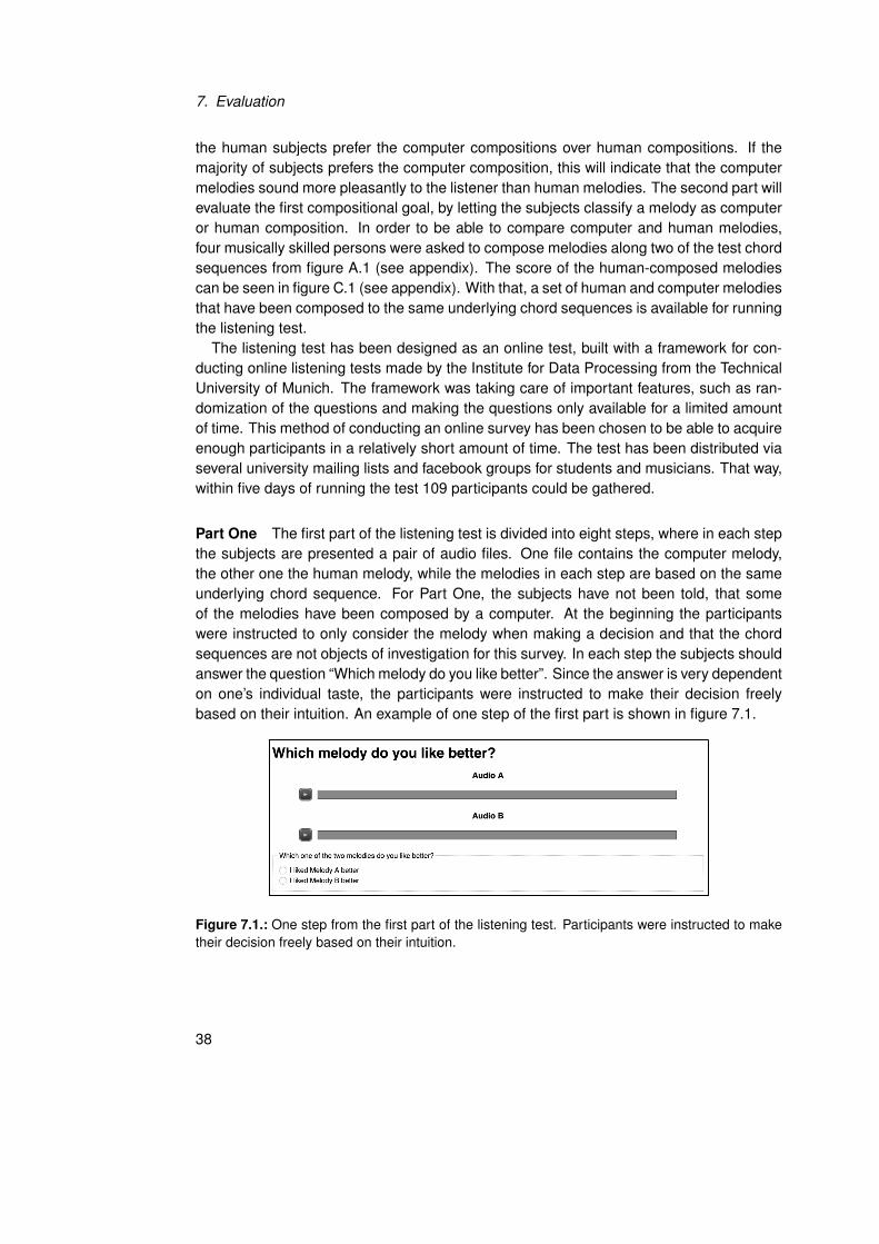
Part One The first part of the listening test is divided into eight steps, where in each stepthe subjects are presented a pair of audio files. One file contains the computer melody,the other one the human melody, while the melodies in each step are based on the sameunderlying chord sequence. For Part One, the subjects have not been told, that someof the melodies have been composed by a computer. At the beginning the participantswere instructed to only consider the melody when making a decision and that the chordsequences are not objects of investigation for this survey. In each step the subjects shouldanswer the question “Which melody do you like better”. Since the answer is very dependenton one’s individual taste, the participants were instructed to make their decision freelybased on their intuition. An example of one step of the first part is shown in figure 7.1.

Figure 7.1.: One step from the first part of the listening test. Participants were instructed to maketheir decision freely based on their intuition.

38

7.1. Subjective Listening Test

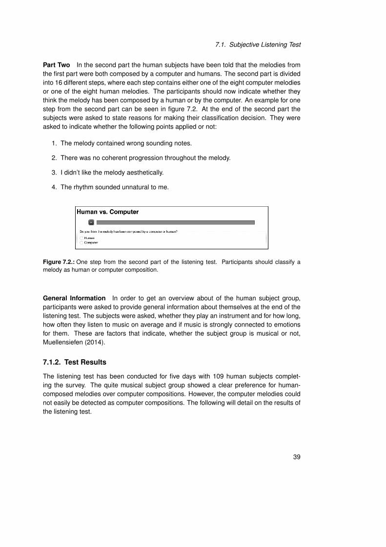
Part Two In the second part the human subjects have been told that the melodies fromthe first part were both composed by a computer and humans. The second part is dividedinto 16 different steps, where each step contains either one of the eight computer melodiesor one of the eight human melodies. The participants should now indicate whether theythink the melody has been composed by a human or by the computer. An example for onestep from the second part can be seen in figure 7.2. At the end of the second part thesubjects were asked to state reasons for making their classification decision. They wereasked to indicate whether the following points applied or not:

1. The melody contained wrong sounding notes.

2. There was no coherent progression throughout the melody.

3. I didn’t like the melody aesthetically.

4. The rhythm sounded unnatural to me.

Figure 7.2.: One step from the second part of the listening test. Participants should classify amelody as human or computer composition.

General Information In order to get an overview about of the human subject group,participants were asked to provide general information about themselves at the end of thelistening test. The subjects were asked, whether they play an instrument and for how long,how often they listen to music on average and if music is strongly connected to emotionsfor them. These are factors that indicate, whether the subject group is musical or not,Muellensiefen (2014).

7.1.2. Test Results

The listening test has been conducted for five days with 109 human subjects complet-ing the survey. The quite musical subject group showed a clear preference for human-composed melodies over computer compositions. However, the computer melodies couldnot easily be detected as computer compositions. The following will detail on the results ofthe listening test.

39

7. Evaluation

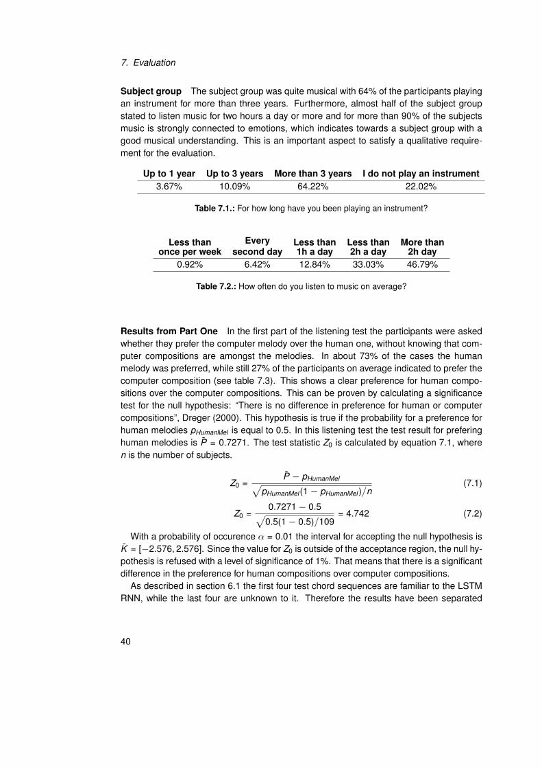
Subject group The subject group was quite musical with 64% of the participants playingan instrument for more than three years. Furthermore, almost half of the subject groupstated to listen music for two hours a day or more and for more than 90% of the subjectsmusic is strongly connected to emotions, which indicates towards a subject group with agood musical understanding. This is an important aspect to satisfy a qualitative require-ment for the evaluation.

Up to 1 year Up to 3 years More than 3 years I do not play an instrument3.67% 10.09% 64.22% 22.02%

Table 7.1.: For how long have you been playing an instrument?

Less thanonce per week

Everysecond day

Less than1h a day

Less than2h a day

More than2h day

0.92% 6.42% 12.84% 33.03% 46.79%

Table 7.2.: How often do you listen to music on average?

Results from Part One In the first part of the listening test the participants were askedwhether they prefer the computer melody over the human one, without knowing that com-puter compositions are amongst the melodies. In about 73% of the cases the humanmelody was preferred, while still 27% of the participants on average indicated to prefer thecomputer composition (see table 7.3). This shows a clear preference for human compo-sitions over the computer compositions. This can be proven by calculating a significancetest for the null hypothesis: “There is no difference in preference for human or computercompositions”, Dreger (2000). This hypothesis is true if the probability for a preference forhuman melodies pHumanMel is equal to 0.5. In this listening test the test result for preferinghuman melodies is P̄ = 0.7271. The test statistic Z0 is calculated by equation 7.1, wheren is the number of subjects.

Z0 =P̄ − pHumanMel√

pHumanMel (1− pHumanMel )/n(7.1)

Z0 =0.7271− 0.5√

0.5(1− 0.5)/109= 4.742 (7.2)

With a probability of occurence α = 0.01 the interval for accepting the null hypothesis isK̄ = [−2.576, 2.576]. Since the value for Z0 is outside of the acceptance region, the null hy-pothesis is refused with a level of significance of 1%. That means that there is a significantdifference in the preference for human compositions over computer compositions.

As described in section 6.1 the first four test chord sequences are familiar to the LSTMRNN, while the last four are unknown to it. Therefore the results have been separated

40

7.1. Subjective Listening Test

into the first four and the last four melodies, to notice that there is no big difference in theresults between this separation. As for the first four melodies in about 26% of the casesthe computer melody was preferred, while this was the case in about 29% of the casesfor the last four melodies. Based on these results, it can be claimed that the LSTM RNNperforms equally well on familiar and unknown chord sequences.

Human melodies preferred Computer melodies preferredAll Testchords 72.71% 27.29%

Testchords 01 to 04 74.08% 25.92%Testchords 05 to 08 71.33% 28.67%

Table 7.3.: The results to the question “Which melody do you like better”. The first row showsthe results over all test chord sequences. The second row only for the test chord sequences withfamiliar chords for the LSTM RNN. The last row only for the unknown test chord sequences.

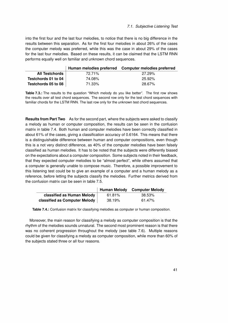
Results from Part Two As for the second part, where the subjects were asked to classifya melody as human or computer composition, the results can be seen in the confusionmatrix in table 7.4. Both human and computer melodies have been correctly classified inabout 61% of the cases, giving a classification accuracy of 0.6164. This means that thereis a distinguishable difference between human and computer compositions, even thoughthis is a not very distinct difference, as 40% of the computer melodies have been falselyclassified as human melodies. It has to be noted that the subjects were differently biasedon the expectations about a computer composition. Some subjects noted in their feedback,that they expected computer melodies to be “almost perfect”, while others assumed thata computer is generally unable to compose music. Therefore, a possible improvement tothis listening test could be to give an example of a computer and a human melody as areference, before letting the subjects classify the melodies. Further metrics derived fromthe confusion matrix can be seen in table 7.5.

Human Melody Computer Melodyclassified as Human Melody 61.81% 38.53%

classified as Computer Melody 38.19% 61.47%

Table 7.4.: Confusion matrix for classifying melodies as computer or human composition.

Moreover, the main reason for classifying a melody as computer composition is that therhythm of the melodies sounds unnatural. The second most prominent reason is that therewas no coherent progression throughout the melody (see table 7.6). Multiple reasonscould be given for classifying a melody as computer composition, while more than 60% ofthe subjects stated three or all four reasons.

41

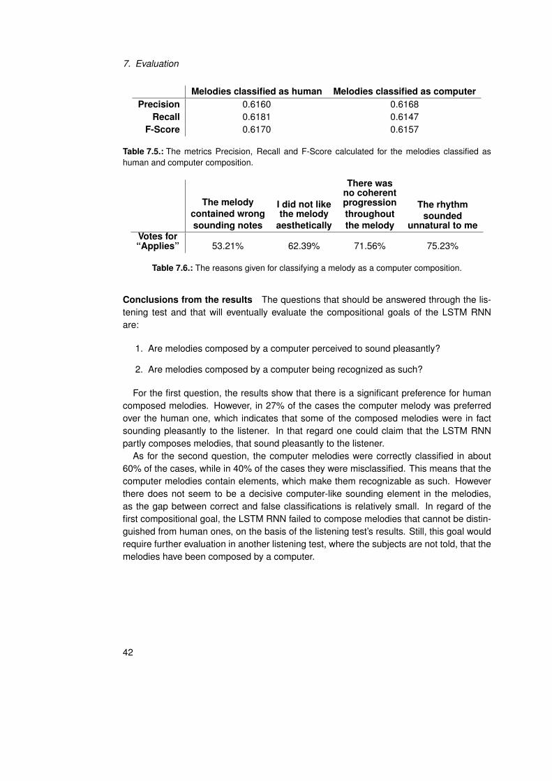
7. Evaluation

Melodies classified as human Melodies classified as computerPrecision 0.6160 0.6168

Recall 0.6181 0.6147F-Score 0.6170 0.6157

Table 7.5.: The metrics Precision, Recall and F-Score calculated for the melodies classified ashuman and computer composition.

The melodycontained wrongsounding notes

I did not likethe melody

aesthetically

There wasno coherentprogressionthroughoutthe melody

The rhythmsounded

unnatural to meVotes for“Applies” 53.21% 62.39% 71.56% 75.23%

Table 7.6.: The reasons given for classifying a melody as a computer composition.

Conclusions from the results The questions that should be answered through the lis-tening test and that will eventually evaluate the compositional goals of the LSTM RNNare:

1. Are melodies composed by a computer perceived to sound pleasantly?

2. Are melodies composed by a computer being recognized as such?

For the first question, the results show that there is a significant preference for humancomposed melodies. However, in 27% of the cases the computer melody was preferredover the human one, which indicates that some of the composed melodies were in factsounding pleasantly to the listener. In that regard one could claim that the LSTM RNNpartly composes melodies, that sound pleasantly to the listener.

As for the second question, the computer melodies were correctly classified in about60% of the cases, while in 40% of the cases they were misclassified. This means that thecomputer melodies contain elements, which make them recognizable as such. Howeverthere does not seem to be a decisive computer-like sounding element in the melodies,as the gap between correct and false classifications is relatively small. In regard of thefirst compositional goal, the LSTM RNN failed to compose melodies that cannot be distin-guished from human ones, on the basis of the listening test’s results. Still, this goal wouldrequire further evaluation in another listening test, where the subjects are not told, that themelodies have been composed by a computer.

42

8. Conclusion

This thesis described a method to compose melodies with LSTM Recurrent Neural Net-works. After giving an overview about the state of the art and an introduction to NeuralNetworks, the implementation of the algorithm was described. The experiments that havebeen done with the implementation were discussed and finally the computer compositionshave been evaluated using human subjects in a listening test.

The main goal for this thesis was to implement a long-short term memory RecurrentNeural Network, that composes melodies that sound pleasantly to the listener and cannotbe distinguished from human melodies. As the evaluation of the computer compositionshas shown, the LSTM RNN composed melodies that partly sounded pleasantly to the lis-tener. However, in the majority of the cases the human compositions were preferred, thusthe LSTM RNN did not fully succeed in fulfilling the first requirement. In addition, the com-puter compositions could be recognized as such in about 60% of the cases, making themdistinguishable from human compositions. Still, in 40% of the cases the computer melodieswere misclassified as human melodies. Overall the LSTM RNN did not succeed in com-pletely fulfilling the main goals for this thesis, but it did in fact compose very interesting andnice sounding melodies at parts, that satisfy those goals.

Further improvements can be applied to the algorithm in order to satisfy the require-ments. For example, more train data could be used as this is very decisive for the qualityof the LSTM RNNs compositions. On top, by defining the compositional goals more specif-ically, the train data can be improved by tailoring it to those goals. The goal of this thesisfor the algorithm was to compose melodies of any kind, however the compositional goalscould be specified to compose melodies within a certain genre, in a certain tempo, etc.Moreover, a different way of representing music apart from the piano roll representationcould improve the algorithm, by letting more versatile musical expressions influence thecomposition process.

A final result is an implementation of a LSTM Recurrent Neural Network, that composesa melody to a given chord sequence, which, apart from any requirements of this thesis,can be used as a creative tool of inspiration for composers and music producers.

43

Appendices

45

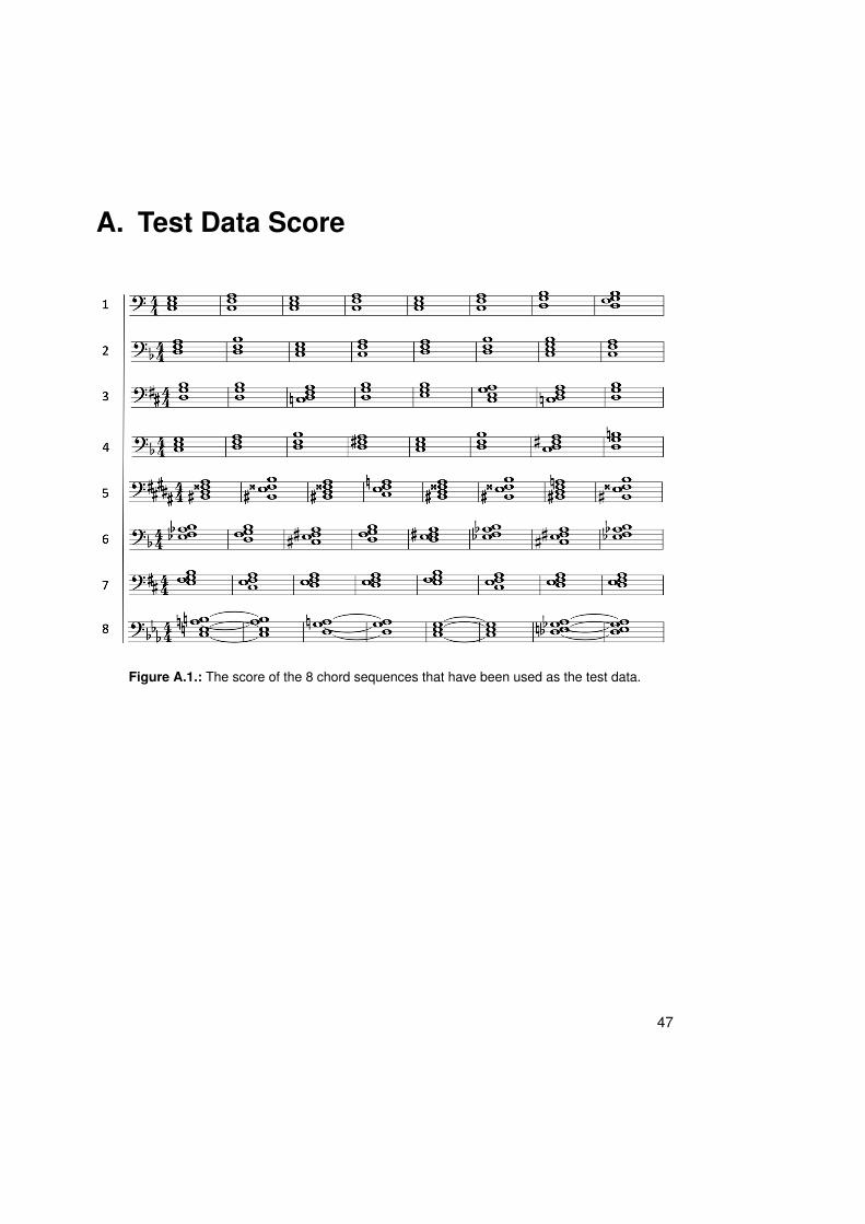
A. Test Data Score

Figure A.1.: The score of the 8 chord sequences that have been used as the test data.

47

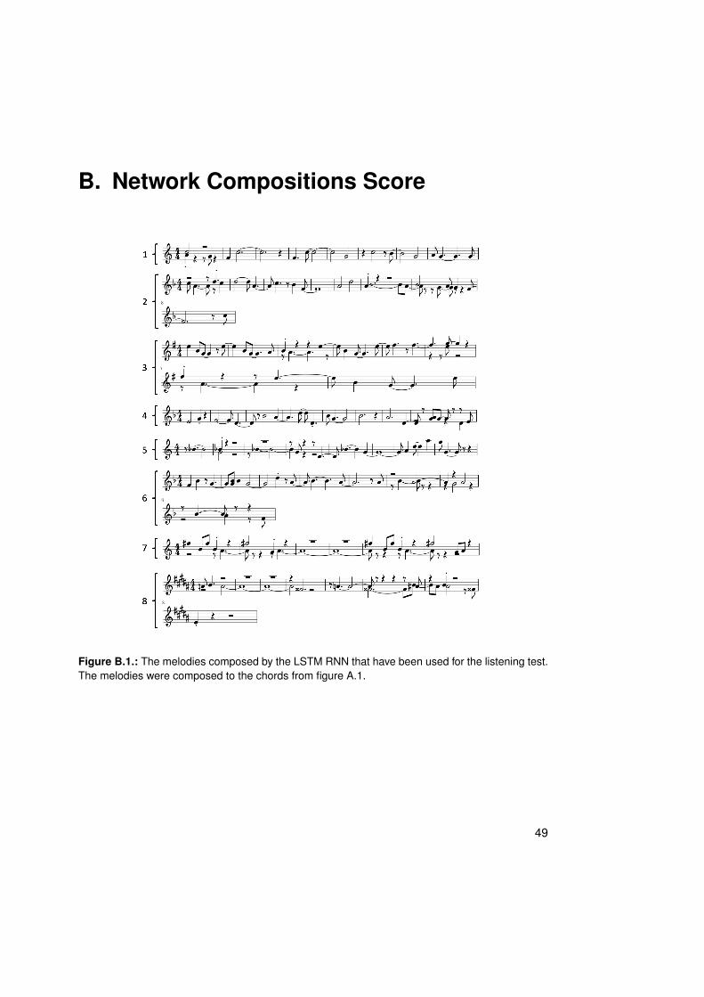
B. Network Compositions Score

Figure B.1.: The melodies composed by the LSTM RNN that have been used for the listening test.The melodies were composed to the chords from figure A.1.

49

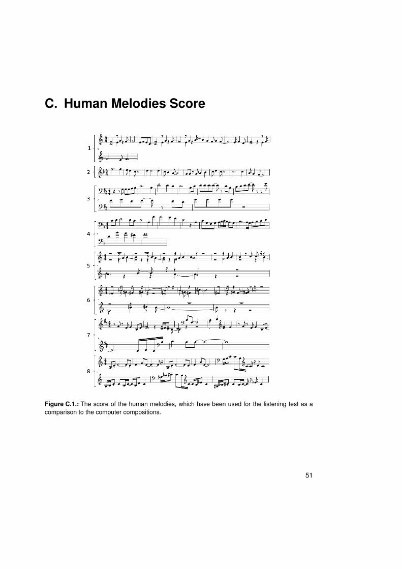
C. Human Melodies Score

Figure C.1.: The score of the human melodies, which have been used for the listening test as acomparison to the computer compositions.

51

Bibliography

Wikipedia: Musical instrument digital interface. 2015. URL https://de.wikipedia.org/wiki/Musical_Instrument_Digital_Interface(lastaccessed:04.11.2015).

L. Bottou. Large-scale machine learning with stochastic gradient descent. In COMP-STAT’2010. 2010.

R. Dean. The Oxford Handbook of Computer Music. Oxford University Press, 2009.

E.K. Dreger. Statistik. Gabler, 2000.

J. Eck, Douglas; Schmidhuber. A First Look at Music Composition using LSTM RecurrentNeural Networks. Technical Report, IDSIA, 2002.

F. Gers. Long short-term memory in recurrent neural networks. In Unpublished PhDdissertation, École Polytechnique Fédérale de Lausanne, Lausanne, Switzerland, 2001.

S. Haykin. A comprehensive foundation. In Neural Networks, 2(2004), 2004.

L. Hiller, Lejaren; Isaacson. Experimental Music - Composition with an electronic com-puter. McGRAW-HILL BOOK COMPANY, 1959.

D. Johnson. Composing music with recurrent neural networks. Au-gust 2015. URL http://www.hexahedria.com/2015/08/03/composing-music-with-recurrent-neural-networks/(lastaccessed:26.10.2015).

D.J. Levitin. Der Musik Instinkt. Spektrum Akademischer Verlag, 2006.

J.E.C. Lipton, Zachary; Berkowitz. In A critical review of recurrent neural networks forsequence learning, 2015.

M. Mozer. Neural network music composition by prediction: Exploring the benefits ofpsychoacoustic constraints and multiscale processing. In Connection Science, 1994.

B.M.J.S.L. Muellensiefen, Daniel; Gingras. The musicality of non-musicians: An index forassessing musical sophistication in the general population. In PLoS ONE 9 e89642. doi10.1371 journal.pone.0089642, 2014.

A. Ng. Lecture notes, sparse autoencoder. 2012a.

53

Bibliography

A. Ng. Lecture notes, supervised learning. 2012b.

G. Nierhaus. Algorithmic Composition - Paradigms of Automated Music Generation.SpringerWienNewYork, 2009.

G. Papadopoulos, George; Wiggins. Ai methods for algorithmic composition: A survey, acritical view and future prospects. In School of Artificial Intelligence, Division of Infor-matics, University of Edinburg.

G. Pearce, Marcus; Wiggins. Towards a framework for the evaluation of machine compo-sitions.

N.L.C. Principe, Jose; Euliano. Neural and Adaptive Systems: Fundamentals ThroughSimulation. 1997.

R. Rojas. Neural Networks, A Systematic Introduction. Springer, 1996.

G.W.R. Rumelhart, David; Hinton. Learning representations by back-propagating errors.In Nature, 1986.

P. da Silva. David cope and experiments in musical intelligence. 2003.

M. Simoni. Algorithmic Composition: A Gentle Introduction to Music Composition Us-ing Common LISP and Common Music. Ann Arbor, University of Michigan Library,http://dx.doi.org/10.3998/spobooks.bbv9810.0001.001, 2003.

J. Stange-Elbe. Computer und Musik: Grundlagen, Technologien und Produktionsumge-bungen der digitalen Musik. De Gruyter Oldenbourg, 2015.

V.P.J. Svozil, Daniel; Kvasnicka. Introduction to multi-layer feed-forward neural networks.In Elsevier, 1997.

F.F. Wilson. Music and mathematics - from pythagoras to fractals. In Oxford UniversityPress, 2003.

S. Windisch. Mathematik zum anfassen - musikalisches wuerfelspiel.

H. Zwicker, Eberhard; Fastl. Psychoacoustics Facts and Models. Springer, 1999.

54