Composites

4 Lectures for Paper B8 Prof. Jin-Chong Tanwww.eng.ox.ac.uk/tan

Michaelmas Term 20151

Department of Engineering Science University of Oxford

Contents of the lectures1. Introduction - engineering applications

2. Basics of two-component composites

3. Elasticity of uni-directional (UD) continuous fibre composites

4. Failure of UD continuous fibre composites

5. Laminated composites: elasticity, bending, twisting and failure

2

e1

e3

e2

eY

eX

eZ

MYXMX

MY

MXY

1. What are composites?

3

• Composite materials are physical mixtures of two or more constituent materials.

e.g. glass fibresmixed into a

polymer resin

Typically, the “particles” have at least two dimensions that are on a small scale (<< 1 mm), visible only under a microscope

• Usually one material forms a continuous matrix, in which particles/fibres of the other material – the “filler” or “reinforcement phase” – are embedded.

200 μm

Fibre–matrix interface

“Microstructure”

Handout P.3

Engineering applications (I)

4

• Advanced composites are used extensively in a wide range of high-tech engineering products

• e.g. in transportation (aircraft, boats, warship), marine structures and sports goods (rackets, rowing eights, fishing rods), amongst many others…

Engineering applications (II)

5

50% composites

Boeing 787 Dreamliner (2011)

High-performance composites

6

• The main reason is that they offer an excellent combination of high specific stiffness (E/ρ)and specific strength (σ*/ρ), and low mass (ρ)

• Composites are being developed based on matrices of metals (MMCs), ceramics (CMCs) and polymers (PMCs)

• But by far the most common composites employed in commercial applications/ manufacturing are those based on polymer matrices (i.e. PMCs)

Typical fibre composite properties (65% fibre + 35% epoxy resin matrix)

7

Density

ρ kg/m3

Modulus

E GPa

Strength

σ* MPa

E/ρ

× 103

σ*/ρ

× 103

Carbon fibre (high

modulus)

1700 222 1630 133 977

Carbon fibre (high

strength)

1600 151 2080 93 1284

Kevlar 49 1400 82 1820 65 1300

E-glass 2100 50 1086 24 515

S-glass 2100 57 1358 27 644

Boron 2100 207 2210 97 1030

polyethylene 970 77 1700 79 1753

Some metals for comparison:

Mild steel 7900 210 450 27 57

Aluminium alloy 2800 70 450 25 161

Titanium 4500 110 960 24 213

“Specific”mechanicalproperties

Handout P.4

A good reinforcement material

8

1. It has high stiffness and strength (UTS)2. It has good particle shape and surface character for

effective mechanical coupling to the matrix3. It preserves the desirable properties of the polymer

matrix (e.g. low shaping T, low conductivities)

The reinforcing action

Handout P.5

Particle aspect ratio

ad

= l Pinningeffect

σ

σ

matrix

particle

What is the optimum size and shapefor a reinforcing particle?

9

( )1 3

2 3 1 32 2/

/ /A a aV V

π −⎛ ⎞= +⎜ ⎟⎝ ⎠

Handout P.6-7

Surface-to-volume ratio of particles:

We want a reinforcement particles to have:(1) high surface area(2) strong bonding to the matrix

Thus we prefer reinforcing particles that are either a << 1 or a >> 1

Also prefer reinforcing particles that are small (i.e. low V), e.g. nanoparticles, exfoliated nano-sheets & nano-clays (1-nm thickness)

aspect ratio a0.01 0.1 1 10 100 1000

A/V in units of (2π/V)1/3

0

5

10

15

20

25

fibreplateletPlatelets Fibres

= l

d

a << 1 a >> 1

Minimum

The major reinforcing fibres

10

• Glass fibres (E-glass, S-glass)• Carbon fibres (HM, HS)• Aramid fibres

(e.g. Kevlar®, Nomex®, Technora®)

Also emerging:• Boron fibres• Polyethylene (PE) fibres

Handout P.8-10

fibreaxis

aromatic polyamide = aramid

Typical fibre properties

11

Density

ρ kg/m3

Axial tensile

modulus E1 GPa

Axial tensile

strength σ* MPa

E-glass 2540 76 1800

S-glass 2490 86 2500

Carbon (HM) 1860 340 2500

Carbon (HS) 1790 230 3200

Kevlar 49 1450 124 2800

Boron (on tungsten) 2600 400 3400

Polyethylene 970 117 2600

Handout P.10

Typical polymer matrix properties

12

Density ρ kg/m3

Tensile modulus E GPa

Tensile strength σ* MPa

Thermoset TS or

thermoplastic TP Epoxy resin 1300 2.4 60 TS

Thermoset polyester 1280 3.0 55 TS

PEEK (Polyether ether ketone)

1390 4.0 90 TP

• Note that whether a matrix is thermoset or a thermoplastic has major implications for manufacturing processes (Production rate? Labour intensive?

Automation?)

Handout P.11

Video: Advanced composites for engineering applications

13

Contents of the lectures1. Introduction - engineering applications

2. Basics of two-component composites

3. Elasticity of uni-directional (UD) continuous fibre composites

4. Failure of UD continuous fibre composites

5. Laminated composites: elasticity, bending, twisting and failure

14

e1

e3

e2

eY

eX

eZ

MYXMX

MY

MXY

Composition

15

Matrix, mass mm , volume vmFiller, mass mf , volume vf

Total mass m and volume v

f mf m f 1v v,

v vϕ ϕ ϕ≡ ≡ = −

( )f f m mf f f m

f m1ρ ϕ ρ ϕ ρ= = ⋅ + ⋅ = + −m v m v m

v v v v v

“Rule of Mixtures” (RoM)

f m f m and in the absence of any holes m m m , v v v= + = +

Handout P.12

Compositedensity

Define:Volume Fractions

Symmetry

16

=x QX

1

1 0 00 1 00 0 1

−⎛ ⎞⎜ ⎟= = ⎜ ⎟⎜ ⎟⎝ ⎠

Q M 1

1 0 00 1 00 0 1

⎛ ⎞⎜ ⎟= = −⎜ ⎟⎜ ⎟−⎝ ⎠

Q R

Quantify symmetry in terms of orthogonal transformations, Q

Symmetry transformations if they leave the object for practical purposes unchanged

1 1

1 0 00 1 00 0 1

−⎛ ⎞⎜ ⎟= = − ≡⎜ ⎟⎜ ⎟−⎝ ⎠

Q M R C

The set of symmetry transformations = G (Symmetry Group)

• Most high-performance composites are anisotropic …• their non-scalar physical properties vary with direction,

and hence with the choice of reference axes.

Mirror symm. 2-fold Rotational symm.

e.g.

Centre of symm.

Handout P.13

..symmetry restriction on response

17

Ae.g. state of ε

Agency Material Response

M Re.g. state of σ

AMR GGG !⊇The principle of “isotropy of space” imposes the restriction

superset Intersection(share a common symm.)

Handout P.14

Basic Mechanics: 2-Component Composite

18

Handout P.15-17

e1e3

e2

σ11 σ11

Area A

Length L

σ11 =ϕ fσ f11 + 1−ϕ f( )σm11

( )11 f f11 f m111ε ϕ ε ϕ ε= + −

Assume L ≈ A d then:

We need “combining rules” for predicting the properties of the composite in terms of the proportions (φ) and properties of 2 constituents

RVE: Volume average stresses & strains in filler and matrix, both of which are homogeneous

Uniaxial loading

d = size of “microstructure”

>>

continuum

Continuum (Macroscopic) Overbar = volume averaged (Microscopic)

..the equations to solve in general

19

f f m m, ij ijkl kl ij ijkl klk l k l

σ ξ σ σ ξ σ= =∑∑ ∑∑

f11 f f f11 f

f22 f f f22 ff

f33 f f f33 f

1 - -1 - 1 -- - 1

TE

ε ν ν σ αε ν ν σ αε ν ν σ α

⎛ ⎞ ⎛ ⎞⎛ ⎞ ⎛ ⎞⎜ ⎟ ⎜ ⎟⎜ ⎟ ⎜ ⎟= + Δ⎜ ⎟ ⎜ ⎟⎜ ⎟ ⎜ ⎟⎜ ⎟ ⎜ ⎟⎜ ⎟ ⎜ ⎟⎝ ⎠ ⎝ ⎠⎝ ⎠ ⎝ ⎠

( ) ( )f f f m f f f m1 1 for all ij ij ij ij ij ij, i , jσ ϕ σ ϕ σ ε ϕ ε ϕ ε= + − = + −

And similarly for an isotropic linear elastic matrix (m)…

Plus constitutive equations (σ-εrelations) of the constituents, e.g. isotropic linear thermo-elastic solid

Handout P.17-19

Continuum stresses —“Applied stresses” onto bulk material

Volume-averaged stresses(overbar) Coupling

coefficients(4-D arrays)

γ f23

γ f31

γ f12

⎛

⎝

⎜⎜⎜⎜

⎞

⎠

⎟⎟⎟⎟

= 1Gf

1 0 00 1 00 0 1

⎛

⎝

⎜⎜

⎞

⎠

⎟⎟

τ f23

τ f31

τ f12

⎛

⎝

⎜⎜⎜⎜

⎞

⎠

⎟⎟⎟⎟

End of Lecture 1

20

Contents of the lectures1. Introduction - engineering applications

2. Basics of two-component composites

3. Elasticity of uni-directional (UD) continuous fibre composites

4. Failure of UD continuous fibre composites

5. Laminated composites: elasticity, bending, twisting and failure

21

e1

e3

e2

eY

eX

eZ

MYXMX

MY

MXY

UD continuous fibre composites

22

e1

e3

e2

• The filler has the form of continuous cylindrical fibresaligned perfectly (along e1),

• .. but located randomly in the plane perpendicular to fibre axes (i.e. isotropic in 2-3 plane).

• Useful when a high degree of reinforcement is required in just one direction

• But more usually they act as building blocks of laminated composites (see later §5), used most widely in engineering composite structures.

e.g.• glass fibres• carbon fibres

Handout P.20

Symmetry in UD composites

23

*Because the fibres are not arranged randomly, this composite will be anisotropic in its physical properties

But it does possess symmetry, as may be expressed in terms of its symmetry group G, which includes

1 1 2

1 0 0 1 0 0 1 0 00 cos sin , 0 1 0 , 0 1 00 sin cos 0 0 1 0 0 1

ω ωω ω

−⎛ ⎞ ⎛ ⎞ ⎛ ⎞⎜ ⎟ ⎜ ⎟ ⎜ ⎟= − = = −⎜ ⎟ ⎜ ⎟ ⎜ ⎟⎜ ⎟ ⎜ ⎟ ⎜ ⎟⎝ ⎠ ⎝ ⎠ ⎝ ⎠

U M M

e1

e3

e2

Handout P.21

U1

M1 M2

isotropic in 2-3 plane

Elastic constants of UD composites

24

Contracted notation for linear elasticity

1 111 11

2 222 22

3 333 33

4 423 23

5 531 31

6 612 12

,

σ εσ εσ εσ εσ εσ ετ γτ γτ γτ γτ γτ γ

⎛ ⎞ ⎛ ⎞⎛ ⎞ ⎛ ⎞⎜ ⎟ ⎜ ⎟⎜ ⎟ ⎜ ⎟⎜ ⎟ ⎜ ⎟⎜ ⎟ ⎜ ⎟⎜ ⎟ ⎜ ⎟⎜ ⎟ ⎜ ⎟

≡ ≡⎜ ⎟ ⎜ ⎟⎜ ⎟ ⎜ ⎟⎜ ⎟ ⎜ ⎟⎜ ⎟ ⎜ ⎟⎜ ⎟ ⎜ ⎟⎜ ⎟ ⎜ ⎟⎜ ⎟ ⎜ ⎟⎜ ⎟ ⎜ ⎟⎜ ⎟ ⎜ ⎟⎜ ⎟ ⎜ ⎟⎝ ⎠ ⎝ ⎠⎝ ⎠ ⎝ ⎠

6

1

ε σ=

=∑p pq qqS

11 12 12

12 22 23

12 23 2244 22 23

44

66

66

0 0 00 0 00 0 0

, where 2( )0 0 0 0 00 0 0 0 00 0 0 0 0

S S SS S SS S S

S S SS

SS

⎛ ⎞⎜ ⎟⎜ ⎟⎜ ⎟

= = −⎜ ⎟⎜ ⎟⎜ ⎟⎜ ⎟⎜ ⎟⎝ ⎠

S

6 x 1 column

matrices

Compliance matrix Slinking strain to stress:

5 independent elastic constants, instead of the usual 2 for isotropic materials

Infinitesimal strain (<5%)

Handout P.22

6 x 6squarematrix

SYMM.

6 x 66 x 1

6 x 1

…in terms of moduli (E, G) and Poisson’s ratios (ν)

25

Handout P.23

12 212 23 23

1 22 (1 ), and E G

E Eν νν= + =

With isotropy in the 2-3 plane

1 1 11 21 2 21 2

1 1 112 1 2 23 2

1 1 112 1 23 2 2

123

112

112

0 0 0

0 0 0

0 0 0

0 0 0 0 0

0 0 0 0 0

0 0 0 0 0

E E E

E E E

E E E

G

G

G

ν νν νν ν

− − −

− − −

− − −

−

−

−

⎛ ⎞− −⎜ ⎟− −⎜ ⎟

⎜ ⎟− −⎜ ⎟= ⎜ ⎟

⎜ ⎟⎜ ⎟⎜ ⎟⎜ ⎟⎝ ⎠

S

SYMM.

Coupling coefficients for UD composite

26

f1 f11 f12 f12 1

f2 f21 f22 f23 2

f3 f21 f23 f22 3

f4 f44 4

f5 f66 5

f6 f66 6

0 0 00 0 00 0 0

0 0 0 0 00 0 0 0 00 0 0 0 0

σ ξ ξ ξ σσ ξ ξ ξ σσ ξ ξ ξ στ ξ ττ ξ ττ ξ τ

⎛ ⎞ ⎛ ⎞⎛ ⎞⎜ ⎟ ⎜ ⎟⎜ ⎟⎜ ⎟ ⎜ ⎟⎜ ⎟⎜ ⎟ ⎜ ⎟⎜ ⎟

=⎜ ⎟ ⎜ ⎟⎜ ⎟⎜ ⎟ ⎜ ⎟⎜ ⎟⎜ ⎟ ⎜ ⎟⎜ ⎟⎜ ⎟ ⎜ ⎟⎜ ⎟⎜ ⎟ ⎜ ⎟⎜ ⎟⎝ ⎠ ⎝ ⎠⎝ ⎠

f fm

f

11

pppp

ϕ ξξ

ϕ−

=− ( )

f fm

f1pq

pqϕ ξ

ξϕ

= −−

From symmetry

From equilibrium

Volume average stresses(induced @ microstruct-ural level of RVE = Response)

fibres

Continuum stresses(applied stresses = Agency)

Stress amplification associated with ξfij(i.e. coupling coefficients)

Handout P.24-25

(p ≠ q)

SYMM.

Axial Tension (1-direction)

27

( ) ( )1 1f1 f11 f f21 f 2 f 3 f21 f f11 f f 21

f f2 ,

E Eσ σε ξ ν ξ ε ε ξ ν ξ ν ξ= − = = − −

( ) ( )

( ) ( )

1m1 f f11 f m f21

f m

1m2 m3 f f21 m f f11 m f f 21

f m

1 2 , 1

11

E

E

σε ϕ ξ ϕ ν ξϕ

σε ε ϕ ξ ν ϕ ξ ν ϕ ξϕ

= − +−

⎡ ⎤= = − + − −⎣ ⎦ −

f1 m1 1ε ε ε= =But ...

Handout P.25-28

• Because of coupling term ξf21, volume average tensile/compressive stresses may be induced in fibres and matrix in directions e2 and e3

• … there is transverse constraint on the f and m in these directions

Fibres:

Matrix:

Strong axial constraint on displacements of fibres and matrix

e1

e3

e2σ1

σ1Axial coupling coeff.

Axial-transverseCoupling coeff.

(compatibility)

Young’s modulus E1 and Poisson’s ratio ν12

28

f 21

f110ξ

ξ→ ( )

ff11

f f f m1E

E Eξ

ϕ ϕ=

+ −Hence…

Note the Rule of Mixtures! (parallel model = equal strain)

• The effect of transverse constraint (ξf21) is much smaller than that of axial constraint (ξf11)

Axial coupling coefficient

Axial tensile modulus

For anisotropic fibres such as carbon or aramid in an isotropic polymer matrix:

( )1 f f f m1E E Eϕ ϕ= + − ( )212 f f f m

11εν ϕν ϕ ν

ε= − = + −

Poisson’s ratio

…take the limit

E1 =ϕ fEf1 + 1−ϕ f( )Em

Transverse Tension

29

Applied stress

Note the complex stress state in matrix

From Hull and Clyne

fibre

matrix

σ

σ

View down the 2-3 plane(isotropic)

e1

e3

e2

σ

σ

2

3

1

2

3

Transverse tension (2-direction)

30

( ) ( )

( )

2 2f1 f12 f f22 f32 f2 f22 f f12 f32

f f

2f3 f32 f f12 f22

f

, ,

E E

E

σ σε ξ ν ξ ξ ε ξ ν ξ ξ

σε ξ ν ξ ξ

⎡ ⎤ ⎡ ⎤= − + = − +⎣ ⎦ ⎣ ⎦

⎡ ⎤= − +⎣ ⎦

( ) ( )

( ) ( )

( ) ( )

2m1 f f12 m f f22 f f32

f m

2m2 f f22 m f f12 f32

f m

2m3 f f32 m f f22 f f12

f m

1 , 1

1 ,1

1 .1

E

E

E

σε ϕ ξ ν ϕ ξ ϕ ξϕσε ϕ ξ ν ϕ ξ ξϕ

σε ϕ ξ ν ϕ ξ ϕ ξϕ

⎡ ⎤= − − − −⎣ ⎦ −

⎡ ⎤= − + +⎣ ⎦ −

⎡ ⎤= − − − −⎣ ⎦ −

• We now need to model the case where a tensile stress is applied in the transverse direction of e2 only (or e3 only)

• There are 3 coupling coefficients involved: ξf12, ξf22, ξf32

Volume average strains for fibres:

.. and for matrix:

Handout P.29

e1

e3

e2

σ2

σ2

Find the transverse modulus E2

31

f32

f120ξ

ξ→ f1 m1 1ε ε ε= =

…gives an equation for the inverse modulus:

…take the limitSince transverseconstraint can be neglected in comparison to axial constraint

We have no means of getting at ξf22without doing a full stress analysis!

Handout P.30

1E2

=ε2σ 2

=ϕ fξf22

Ef+

1−ϕ fξf22( )Em

−ϕ f 1−ϕ f( )EfEm

ϕ fEf + 1−ϕ f( )Em

ν fEf

−νmEm

⎛

⎝⎜⎞

⎠⎟ν fξf22

Ef−νmEm

1−ϕ fξf22( )1−ϕ f( )

⎛

⎝⎜

⎞

⎠⎟

(compatibility)

..but we may employ approximations

32

f22 1ξ =

( ) ( )( )

2f f f f mf f m

2 f m f f f m f m

1 111E E

E E E E E E Eϕ ϕ ϕϕ ν ν

ϕ ϕ− − ⎛ ⎞

= + − −⎜ ⎟+ − ⎝ ⎠

1. With

we get

2. With

we get

and f12 0ξ =

f22 1ξ =

The Inverse Rule of Mixtures

( )ff

2 f m

11E E E

ϕϕ −= +

assume no stress amplification

under-estimated since ξf22 >1 in reality

assume noaxial constraint

Handout P.31

under-estimate even more than assumption #1 above

(series model = equal stress)

(3.26)

Alternative, empirical approach

33

3. The “Halpin-Tsai” (H-T) equations for property p

If p = E2 then it is found ζ ~1

f f mm

f f m

1 / 1 where =1- /

p pp pp p

ζηϕ ηηϕ ζ

⎛ ⎞+ −= ⎜ ⎟ +⎝ ⎠

Handout P.32

Comparison of the models

34

à Assume no stress amplification

Assume no stress amp.& no axial constraint

à Empirical approach

φ beyond 70% not achievable in practice

Handout P.33

A typical UD composite of glass fibres in epoxy resin

f22 1ξ =

Halpin-Tsai (H-T) model against some experimental data

35

Inverse RoM(equal stress = Lower Bound)

RoM parallel model(equal strain = Upper Bound)

H-T equation ζ ~1

From Hull and Clyne

Handout P.34

e1

e3

e2

Shear modulus parallel to fibres: G12 or G13

36

6 f f66 f f66

12 6 f m

11G G G

γ ϕ ξ ϕ ξτ

−= = +

Again the same options:

1. Assume something about the coupling, e.g. ξ66 =1 gives

2. Apply Halpin-Tsai (H-T) equation with ζ = 1

f f m12 m

f f m

1 / 1 where 1- / 1

G GG GG G

ηϕ ηηϕ

⎛ ⎞ ⎛ ⎞+ −= =⎜ ⎟ ⎜ ⎟+⎝ ⎠ ⎝ ⎠

Handout P.35

f f

12 f m

11G G G

ϕ ϕ−= +

Composite sheared in the 1-2 plane

Degree of stress amplification in the fibres ξf66

e1

e3

e2Inverse RoM

τ12

τ12

Fibre volume fraction φf

0.0 0.2 0.4 0.6 0.8

Shea

r mod

ulus

G12

GPa

0

1

2

3

4

5

6Stress am

plification ξf66

0.0

0.5

1.0

1.5

2.0

Inverserule ofmixtures

H-T equation

Comparison of inverse rule of mixtures and H-T equation

37

Handout P.37

(lower bound)

Thermal expansion

38

Handout P.37

σf1

σf2

σf3

τ f4

τ f5

τ f6

⎛

⎝

⎜⎜⎜⎜⎜⎜⎜⎜⎜⎜⎜⎜⎜⎜⎜⎜⎜⎜⎜⎜⎜⎜

⎞

⎠

⎟⎟⎟⎟⎟⎟⎟⎟⎟⎟⎟⎟⎟⎟⎟⎟⎟⎟⎟⎟⎟⎟⎟⎟⎟

=

ξf1T

ξf2T

ξf2T

000

⎛

⎝

⎜⎜⎜⎜⎜⎜⎜⎜⎜⎜⎜⎜⎜⎜⎜⎜⎜⎜⎜

⎞

⎠

⎟⎟⎟⎟⎟⎟⎟⎟⎟⎟⎟⎟⎟⎟⎟⎟⎟⎟⎟⎟⎟⎟

ΔT

( )f

m T f Tf

( 1..3)1p p pϕξ ξ

ϕ= − =

−

A temperature rise ΔT gives rise to internal stresses due to thermal expansion mismatch between fibre and matrix…

where…

Stress-temperature coupling factors ξfpT(p = 1..6) relate the induced mean stress in the fibres to the temperature rise of the composite ΔT

stress amplification factors in the matrixfrom equilibrium

Due to symmetry, only two independentcoupling coefficients ξf1T and ξf2T

… and hence to internal strains

39

( ) ( )f1 f1T f f2T f f f2 f3 f f2T f f1T f ff f

2 , 1T TE EE E

ε ξ ν ξ α ε ε ν ξ ν ξ αΔ Δ⎡ ⎤= − + = = − − +⎣ ⎦

f1 m1ε ε=f2T

f1T0ξ

ξ→

Then take the limit…

We get…

( )f f f f m mf11

1

1E ET E

ϕ α ϕ αεα+ −

= =Δ

( ) ( ) ( )2 f f f f m m 1 121 1 1α ϕ α ν ϕ α ν αν= + + − + −

Handout P.38-39

Axial coefficient of thermal expansion (CTE)

Transverse CTE

Axial strain Transverse strains

(compatibility)

Anisotropy of thermal expansion

40Fibre volume fraction φf

0.0 0.2 0.4 0.6 0.8 1.0

Thermal expansion coefficient x 106

K-1

01020304050607080

α2

α1

Handout P.40

• These calculations of CTEs fit experimental data rather well

• It can be seen that:α2 > α1

Why?

e.g. UD glass/epoxy composite

End of Lecture 2

41

Contents of the lectures1. Introduction - engineering applications

2. Basics of two-component composites

3. Elasticity of uni-directional (UD) continuous fibre composites

4. Failure of UD continuous fibre composites

5. Laminated composites: elasticity, bending, twisting and failure

42

e1

e3

e2

eY

eX

eZ

MYXMX

MY

MXY

4. Failure of UD Fibre Composites

43

Handout P.41

asterisk “ * ” denotes failure

In most polymer matrix composite materials, both the fibres and the matrix are relatively brittle: they fracture in tension at small strains ε*after little or no detectable plastic deformation

Fibre type Failure strain ε*

Glass 0.02-0.03

Carbon (HM) ~0.005

Carbon (HS) ~0.01

Kevlar 49 ~0.025

Matrix type Failure strain ε*

Epoxy resin 0.02-0.05

Thermoset polyester ~0.02

ε* < ~5%

…but fibre pull-out increases toughness

44

Handout P.42

crack

fibre

matrix

• What’s the toughening mechanism? - When a crack grows in the matrix and approaches a fibre, the

interface is sheared. - If the interface is weak, it fails in shear and the crack turns and runs

along the fibre, - ..until it finds a relatively weak spot on the fibre where that breaks,

and so on until the composite is completely broken.

• Weak fibre-matrix interfaces act as crack-stoppers

Fibrebridging

Fracture surface under a Scanning Electron Microscope (SEM)

45

A glass/polyester composite with

weak interfacesσ

σ• Pull-out of partially-debonded fibres from a fracture plane absorbs energy.

• Hence composite materials (especially those with weak interfaces) can be tougher than their constituent materials.

From Hull and Clyne

Calculation of tensile strength σ1*parallel to fibres (1-direction)

46

f m* *ε ε<

m f* *ε ε<

2 cases to consider:

Case I

Case II

Handout P.42

the fibres are more brittle than the matrix

the matrix is more brittle than the fibres

where ε* denotes failure strain

Case I: εf* < εm*e.g. high modulus carbon fibres (~1%)

in epoxy resin matrix (2~5%)

47

Strain

Stress

εm*εf*

σm’σm*

σf*

Matrix

Fibres

Stress carried by matrix at the failure strain of fibres (denoted by ’ )

Handout P.42

(relatively more brittle)

…again two possible cases

48

Strain

Stress

εm*εf*

(1−φ σf m) *

φσf f*

Matrix

Fibres

Composite

Strain

Stress

εm*εf*

φσf f*

Matrix

Fibres

Composite

(1−φ σf m) ’

σ1∗

( )1 f f f m* * 1 'σ ϕ σ ϕ σ= + −( )1 f m* 1 *σ ϕ σ= −

Handout P.43-44

Tensile strength at failure - the matrixis carrying all the stress alone!

ϕ <<f 1 At higher φf(Few %)

Which one wins?

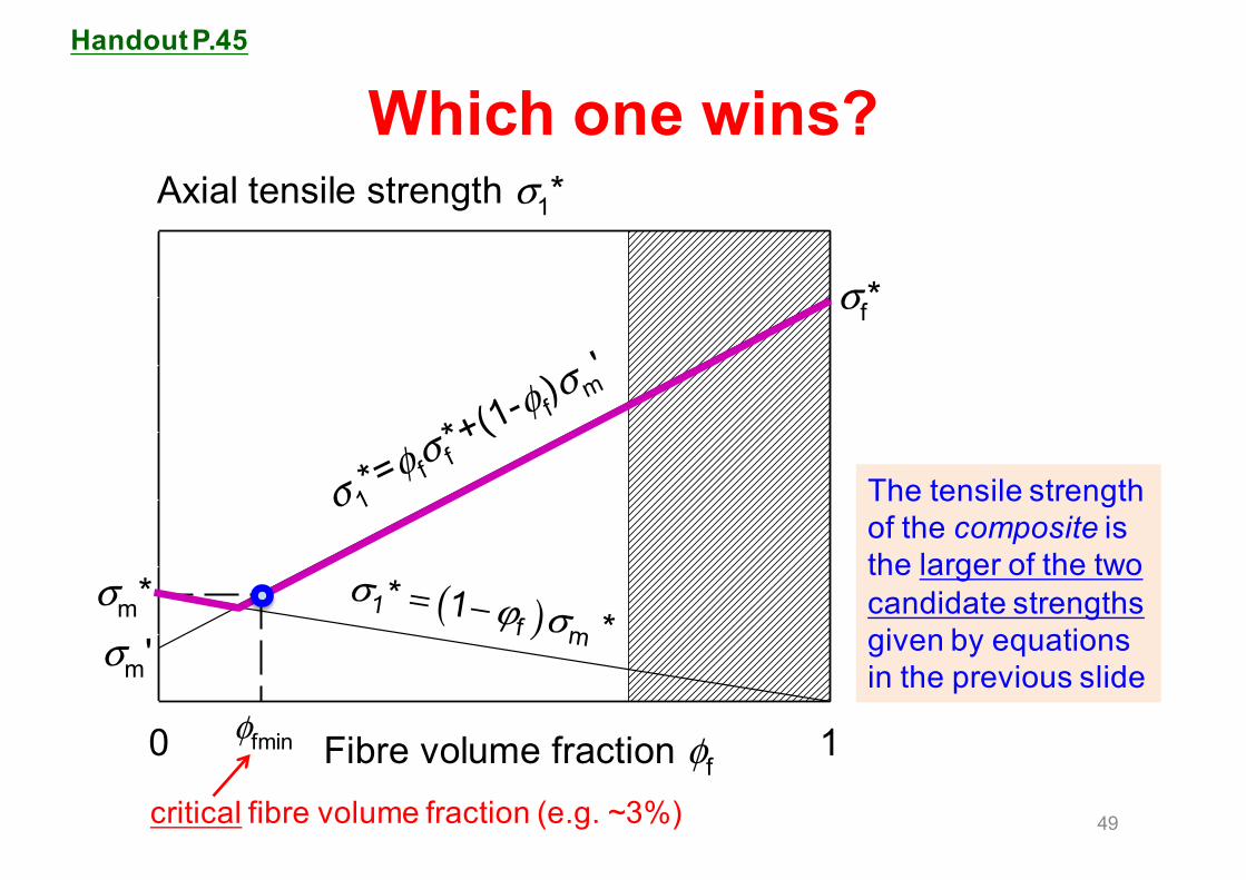
49

Fibre volume fraction φf0 1

Axial tensile strength σ1*

0

50

100

150

200

250

300

350

σm*σm'

σf*

σ 1*=φ fσ f*+

(1-φ f)σ m'

σ1*=φfσm*

φfmin

The tensile strength of the composite is the larger of the two candidate strengths given by equations in the previous slide

critical fibre volume fraction (e.g. ~3%)

Handout P.45

( )1f m

* 1 *σ ϕ σ= −

Case II: εf* > εm*e.g. glass fibres (2~3%) in a

thermoset polyester matrix (~2%)

50

Strain

Stress

εm* εf*

σf’

σm*

σf*

Matrix

Fibres

(relatively more brittle)

Stress carried by fibres at the failure strain of matrix (denoted by ’ )

Handout P.46

…and again two cases

51

Strain

Stress

εm* εf*

(1−φ σf m) *

φσf f’

Matrix

Fibres

Compositeσ1*

1 f f f m* ' (1 ) *σ ϕ σ ϕ σ= + −

Strain

Stress

εm* εf*(1−φ σf m) * Matrix

Fibres

Compositeφσf f*

1 f f* *σ ϕ σ=

f 1ϕ <<

Handout P.46-47

At higher φf(Few %)

Which one wins this time?

52

Fibre volume fraction φf0 1

Axial tensile strength σ1*

0

50

100

150

200

250

300

350

σm*

σf'

σf*

σ1*=φfσf'+(1-φf)σm*

σ 1*=φ fσ f*

Handout P.47

Other modes of failure

53

σ2T*

Axial compression

Transverse tension

Axial shear

σ2T*

Handout P.48-50

σ1C*

τ12*

Shear bands

Stress concentratorsat fibre tips

e1

eX

eY

θσ

Failure under off-axis stress

54

Handout P.50

e.g. off-axis tension

We need an anisotropic failure criterion

e.g. “Maximum Stress” failure criterion

1211 11 22 22

1T 1C 2T 2C 12MAX , , , , 1

* * * * *τσ σ σ σ

σ σ σ σ τ⎛ ⎞− − ≥⎜ ⎟⎝ ⎠

σσ

• The idea is that the various failure modes outlined in the previous slide are assumed to be separate and non-interacting

• Failure will occur when the following condition is first satisfied:

Failure criterion in example P.53

55

2 2

1 2 12

cos sin sin cosMAX , , 1* * *

σ θ σ θ σ θ θσ σ τ

⎛ ⎞≥⎜ ⎟

⎝ ⎠

Angle θ degrees

0 10 20 30 40 50 60 70 80 90

Tens

ile s

treng

th σ*

0

200

400

600

800

A B C

A = axial tensile failureB = axial shear failureC = transverse tensile failure

axial tension

axialshear transverse

tension

Failure modes

Data for 50% glass fibres in polyester resin

Handout P.53

T T

Contents of the lectures1. Introduction - engineering applications

2. Basics of two-component composites

3. Elasticity of uni-directional (UD) continuous fibre composites

4. Failure of UD continuous fibre composites

5. Laminated composites: elasticity, bending, twisting and failure

56

e1

e3

e2

eY

eX

eZ

MYXMX

MY

MXY

Lamina or “ply”

5. Laminated Composites

57

Handout P.54

• UD fibre composites can offer high values of specific strength and stiffness parallel to the fibres,

• ..but such composites are highly anisotropic with poor transverse mechanical properties

• Hence we create a laminate of UD composites to withstand biaxial and triaxial stress states.

e.g. a 3-layer laminatewith stacking sequenceof [0/90/0]

Global co-ordinate axes with O at centre of laminate: eX eY eZLocal co-ordinate axes within a single lamina e1 e2 e3

O

Stacking sequence notation (I)

58

[ ]1 2 3/ / / nθ θ θ θ⋅ ⋅ ⋅ ⋅ ⋅

[ ] [ ] [ ]2 20 / 90 /0 0/90 /90/ 0 , 0/90/0 [0 / 90 /0 /0 / 90/0]≡ ≡

[ ] [ ]0 / 30 / 0 0 / 30 / 30 /0± ≡ + −

[ ] [ ] [ ]2s0 / 90 0/90 /90/ 0 0 /90 / 0≡ =

General stacking sequence:

Multiple adjacent plies

Balancing plies

Symmetrically arranged plies

Handout P.55

Stacking sequence notation (II)

59

These abbreviations can be combined, to enable complex stacking sequences to be expressed compactly

Handout P.56

0 / ±30⎡⎣ ⎤⎦2s≡ 0 / +30 / −30⎡⎣ ⎤⎦2s

≡ 0 / +30 / −30 / 0 / +30 / −30⎡⎣ ⎤⎦s

≡ 0 / +30 / −30 / 0 / +30 / −30 / −30 / +30 / 0 / −30 / +30 / 0⎡⎣ ⎤⎦

Eqn.(5.5) Mirror plane (Mz)

≡ A laminate stack of 12 plies (laminae)

Symmetry of laminates

60

• “Symmetric” laminates exhibit mirror symmetry in the mid-plane (Mz), i.e.

• “Balanced” laminates have equal numbers of

+θ and -θ plies

Handout P.56-57

[ ]1 2 3 s/ / ... mθ θ θ θLaminate has 2m of plies and cannot undergo out-of-plane deformation: i.e. it cannot bend or twist

No tension—shear coupling in the plane of eX and eY, when in-plane loads or displacements are applied parallel or perpendicular to these axesBalanced, symmetric plies are

preferred in practice.

Laminate elasticity – single lamina (ply) stresses

61

Laminates mostly experience plane stress conditions (h << 1 mm).

The strain-stress relation is then

[ ]

21

1 2

12

1 2

12

1 0

1 0

10 0

E E

SE E

G

ν

ν

⎡ ⎤−⎢ ⎥⎢ ⎥⎢ ⎥−= ⎢ ⎥⎢ ⎥⎢ ⎥⎢ ⎥⎢ ⎥⎣ ⎦

And we recall….

Handout P.58

“Reduced compliance matrix” [S] of the lamina

ε1

ε2

γ 6

⎛

⎝

⎜⎜⎜⎜

⎞

⎠

⎟⎟⎟⎟

=

S11 S12 0

S21 S22 0

0 0 S66

⎡

⎣

⎢⎢⎢⎢

⎤

⎦

⎥⎥⎥⎥

σ1

σ 2

τ6

⎛

⎝

⎜⎜⎜⎜

⎞

⎠

⎟⎟⎟⎟

3 x 3

e1

e3

e2

τ6 = τ12σ1 σ2

σ3 = 0

(σ3 = 0)

symm

RECAP à Compliance Matrix [S]

62

1 111 11

2 222 22

3 333 33

4 423 23

5 531 31

6 612 12

,

σ εσ εσ εσ εσ εσ ετ γτ γτ γτ γτ γτ γ

⎛ ⎞ ⎛ ⎞⎛ ⎞ ⎛ ⎞⎜ ⎟ ⎜ ⎟⎜ ⎟ ⎜ ⎟⎜ ⎟ ⎜ ⎟⎜ ⎟ ⎜ ⎟⎜ ⎟ ⎜ ⎟⎜ ⎟ ⎜ ⎟

≡ ≡⎜ ⎟ ⎜ ⎟⎜ ⎟ ⎜ ⎟⎜ ⎟ ⎜ ⎟⎜ ⎟ ⎜ ⎟⎜ ⎟ ⎜ ⎟⎜ ⎟ ⎜ ⎟⎜ ⎟ ⎜ ⎟⎜ ⎟ ⎜ ⎟⎜ ⎟ ⎜ ⎟⎜ ⎟ ⎜ ⎟⎝ ⎠ ⎝ ⎠⎝ ⎠ ⎝ ⎠

11 12 12

12 22 23

12 23 2244 22 23

44

66

66

0 0 00 0 00 0 0

, where 2( )0 0 0 0 00 0 0 0 00 0 0 0 0

S S SS S SS S S

S S SS

SS

⎛ ⎞⎜ ⎟⎜ ⎟⎜ ⎟

= = −⎜ ⎟⎜ ⎟⎜ ⎟⎜ ⎟⎜ ⎟⎝ ⎠

S

Recap — Handout P.22-23

6 x 6

Plane stress (3 x 1)

6 x 11 1 1

1 21 2 21 21 1 1

12 1 2 23 21 1 1

12 1 23 2 2123

112

112

0 0 0

0 0 0

0 0 0

0 0 0 0 0

0 0 0 0 0

0 0 0 0 0

E E E

E E E

E E E

G

G

G

ν νν νν ν

− − −

− − −

− − −

−

−

−

⎛ ⎞− −⎜ ⎟− −⎜ ⎟

⎜ ⎟− −⎜ ⎟= ⎜ ⎟

⎜ ⎟⎜ ⎟⎜ ⎟⎜ ⎟⎝ ⎠

S

Reduced compliance matrix (3 x 3 sub-matrix)

6 x 1

In-plane strains (3 x 1)

SYMM.

The reduced (plane stress) stiffness matrix [Q] of a single lamina

63

Inverting the 3x3 [S] sub-matrix we obtain:

( ) ( )

( ) ( )

1 21 1

12 21 12 21

1 12 2 2

12 21 12 21

12

01 1

[ ] [ ] 01 1

0 0

E E

E EQ S

G

νν ν ν ν

νν ν ν ν

−

⎡ ⎤⎢ ⎥− −⎢ ⎥⎢ ⎥

= = ⎢ ⎥− −⎢ ⎥⎢ ⎥⎢ ⎥⎢ ⎥⎣ ⎦

Handout P.58

Note: 1. [Q] is the stiffness of a single lamina w.r.t. local axes e1 & e2

2. Applicable only under plane stress conditions

SYMM.

In a single lamina (one ply)…

64

• The stresses are related to the in-plane strains by

[ ]1 1

2 2

6 6

Qσ εσ ετ γ

⎛ ⎞ ⎛ ⎞⎜ ⎟ ⎜ ⎟=⎜ ⎟ ⎜ ⎟⎜ ⎟ ⎜ ⎟⎝ ⎠ ⎝ ⎠

• In general, local axes e1, e2 of lamina will be inclinedto the global axes eX, eY, by an angle θ

Handout P.59

e1

eX

eY

θσRecap:

Handout P.50 σσ

3 x 3 3 x 13 x 1

Local axes1-2 plane

Rotation of axes of [Q] via Mohr’s circle

65

1 XX 1 XX

2 YY 2 YY

6 XY 6 XY

[ ] , [ ]T Tσ ε

σ σ ε εσ σ ε ετ τ γ γ

⎛ ⎞ ⎛ ⎞ ⎛ ⎞ ⎛ ⎞⎜ ⎟ ⎜ ⎟ ⎜ ⎟ ⎜ ⎟= =⎜ ⎟ ⎜ ⎟ ⎜ ⎟ ⎜ ⎟⎜ ⎟ ⎜ ⎟ ⎜ ⎟ ⎜ ⎟⎝ ⎠ ⎝ ⎠ ⎝ ⎠ ⎝ ⎠

2 2 2 2

2 2 2 2

2 2 2 2

2

[ ] 2 , [ ]( ) 2 2 ( )

c s cs c s cs

T s c cs T s c cs

cs cs c s cs cs c sσ ε

⎡ ⎤ ⎡ ⎤⎢ ⎥ ⎢ ⎥

= − = −⎢ ⎥ ⎢ ⎥⎢ ⎥ ⎢ ⎥− − − −⎢ ⎥ ⎢ ⎥⎣ ⎦ ⎣ ⎦

XX 1 1 XX1 1 1

YY 2 2 YY

XY 6 6 XY

[ ] [ ] [ ] [ ] [ ][ ]T T Q T Q Tσ σ σ ε

σ σ ε εσ σ ε ετ τ γ γ

− − −⎛ ⎞ ⎛ ⎞ ⎛ ⎞ ⎛ ⎞⎜ ⎟ ⎜ ⎟ ⎜ ⎟ ⎜ ⎟= = =⎜ ⎟ ⎜ ⎟ ⎜ ⎟ ⎜ ⎟⎜ ⎟ ⎜ ⎟ ⎜ ⎟ ⎜ ⎟⎝ ⎠ ⎝ ⎠ ⎝ ⎠ ⎝ ⎠

Hence..

• To calculate the response of the whole laminate,

• first we need to establish σ-εrelation for each layer,

• .. expressed w.r.t. the globalreference axes along X, Y, Z Global

(≡ Laminate)Local

(≡ Lamina)

c ≡ cosθ, s ≡ sinθ

Handout P.60-61

GlobalGlobal Local Local

Transformation matrices to convert stress and strain:

Q⎡⎣ ⎤⎦

Global(≡ Laminate)

Local(≡ Lamina)

result… Lamina Stiffness Matrix [Q]

66

XX XX1

YY YY

XY XY

[ ] where [ ] [ ] [ ][ ]Q Q T Q Tσ ε

σ εσ ετ γ

−⎛ ⎞ ⎛ ⎞⎜ ⎟ ⎜ ⎟= =⎜ ⎟ ⎜ ⎟⎜ ⎟ ⎜ ⎟⎝ ⎠ ⎝ ⎠

4 4 2 211 11 22 12 662( )Q Q c Q s Q Q c s= + + +

3 316 11 12 66 12 22 66( 2 ) ( 2 )Q Q Q Q c s Q Q Q cs= − − + − +

4 4 2 266 66 11 22 12 66( ) ( 2 2 )Q Q c s Q Q Q Q c s= + + + − −

Handout P.60

The lamina stress-strain relation, expressed with respect to the global (laminate) reference axes (eX, eY, eZ)

=

Q11 Q12 Q16

Q12 Q22 Q26

Q16 Q26 Q66

⎡

⎣

⎢⎢⎢⎢

⎤

⎦

⎥⎥⎥⎥ 3 x 3

Examples of some terms in [Q]:

Eqn.(5.16-5.21)

Laminate forces N (unit load: N/m)

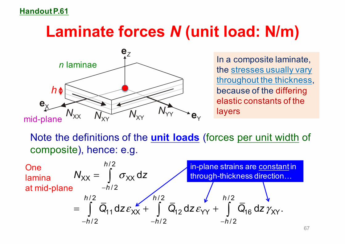
67

eXeY

eZ

NXY NXY NYYNXX

Note the definitions of the unit loads (forces per unit width of composite), hence: e.g.

/ 2

XX XX/ 2

/ 2 / 2 / 2

11 XX 12 YY 16 XY/ 2 / 2 / 2

d

d d d .

h

hh h h

h h h

N z

Q z Q z Q z

σ

ε ε γ

−

− − −

=

= + +

∫

∫ ∫ ∫

Handout P.61

In a composite laminate, the stresses usually vary throughout the thickness, because of the differing elastic constants of the layers

in-plane strains are constant in through-thickness direction…

mid-plane

h

n laminae

Onelaminaat mid-plane

Summing over the n laminae…

68

( )

( )

( )

XX 11 1 XX1

12 1 YY1

16 1 XY1

( )

( )

( ) .

n

k k kk

n

k k kk

n

k k kk

N Q h h

Q h h

Q h h

ε

ε

γ

−=

−=

−=

= −

+ −

+ −

∑

∑

∑

Handout P.62

hk

eZ

eXk

1mid-plane

..the integrals can be replaced by summations over the n layers

Seen edgewise:(down eY)

n layers

..giving the laminate stiffness matrix [A]

69

Handout P.63

where…

( )11( )

n

ij ij k k kk

A Q h h −=

= −∑

• Repeat the step in previous slide to obtain similar expressions for the other unit loads NYY and NXY

• ... can be combined in the form of a matrix equation relating the unit loads {N} to the laminate in-plane strains {ε}:

NXX

NYY

NXY

⎛

⎝

⎜⎜⎜⎜

⎞

⎠

⎟⎟⎟⎟

=

A11 A12 A16

A12 A22 A26

A16 A26 A66

⎡

⎣

⎢⎢⎢⎢

⎤

⎦

⎥⎥⎥⎥

εXX

εYY

γ XY

⎛

⎝

⎜⎜⎜⎜

⎞

⎠

⎟⎟⎟⎟

the thickness of the k-thlamina

SYMM.

Global systemX, Y, Z

Steps in laminate calculations…

70

A typical problem in the mechanics of fibre composite laminates would be: a laminate is to be subjected to certain in-plane strains εXX, εYY, γXY, predict the unit loads induced.

Handout P.63

1. For each lamina, obtain the elastic constants:

2. For each lamina calculate matrix [Q] (Local axes)

3. For each lamina rotate axes to obtain (Global axes)

4. For the whole laminate calculate [A]

5. Multiply the strain column by [A] to obtain the unit loads {N}

1 2 12 21 12, , , , E E Gν ν

[ ]QUsing eqn.(5.16-5.21)

Laminate example #1

71

Laminate example 1: Calculate the stiffness matrix [A] for a [+45/-45]s

laminate constructed from 4 identical laminae each with thickness 0.1 mm

and with elastic constants:

1 2 12 1255 GPa, 16 GPa, 0.28, 7.6 GPa.E E Gν= = = =

Handout P.65

Contents of the lectures1. Introduction - engineering applications

2. Basics of two-component composites

3. Elasticity of uni-directional (UD) continuous fibre composites

4. Failure of UD continuous fibre composites

5. Laminated composites: elasticity, bending, twisting and failure

72

e1

e3

e2

eY

eX

eZ

MYXMX

MY

MXY

Laminate bending and twisting

73

eY

eX

eZ

MYXMX

MY

MXY

We define unit moments as shown

Handout P.67

To retain the usual sign convention (sagging bending moments are positive); we view the laminate from underneath (+eZ pointing down).

Bending moments per unit width of laminate

Twisting moments per unit width of laminate

Special case: bending in the X-Z plane

74

MX MX

h

eZ

eX

XX X

YY

XY

00

kz

εεγ

⎛ ⎞ ⎛ ⎞⎜ ⎟ ⎜ ⎟=⎜ ⎟ ⎜ ⎟⎜ ⎟ ⎜ ⎟⎝ ⎠ ⎝ ⎠

/ 2 / 22

X XX 11 X/ 2 / 2

d dh h

h h

M z z Q z zkσ− −

= =∫ ∫

For curvature kX (=1/R) the strains:

Hence the bending moment in the XZ plane:

Handout P.67

Curvature in XZ plane

Plane strain

Not twisting

A wide plateA special case:

z

The general case of bending/twisting

75

XX X

YY Y

XY XY

kz kk

εεγ

⎛ ⎞ ⎛ ⎞⎜ ⎟ ⎜ ⎟=⎜ ⎟ ⎜ ⎟⎜ ⎟ ⎜ ⎟⎝ ⎠ ⎝ ⎠

( )

( )

( )

3 3X 11 1 X

1

3 312 1 Y

1

3 316 1 XY

1

1 ( )3

1 ( )3

1 ( ) .3

n

k k kk

n

k k kk

n

k k kk

M Q h h k

Q h h k

Q h h k

−=

−=

−=

= −

+ −

+ −

∑

∑

∑

Handout P.68

..and the bending moment in the XZ plane becomes

As before, we recognise that the elements of [Q] are piecewise constant through the thickness of the laminate, resulting in summations over the n laminae as follows

twisting curvature

curvature in YZ plane curvature in XZ plane

The bending/twisting stiffness matrix for the laminate [D]

76

X 11 12 16 X

Y 12 22 26 Y

XY 16 26 66 XY

M D D D kM D D D kM D D D k

⎛ ⎞ ⎛ ⎞⎛ ⎞⎜ ⎟ ⎜ ⎟⎜ ⎟=⎜ ⎟ ⎜ ⎟⎜ ⎟⎜ ⎟ ⎜ ⎟⎜ ⎟⎝ ⎠ ⎝ ⎠⎝ ⎠

where

( )3 31

1

1 ( )3

n

ij ij k k kk

D Q h h −=

= −∑

Handout P.69

When this step is repeated for the YZ plane moment MY and twisting moment MXY (=MYX), the complete set of bending moments may be expressed as

SYMM.

The case of the symmetric laminate

77

eZ

eX

Stress )σ (XX z

StrainεXX( )z

MX MX

Answer : there is no net axial force

Handout P.70

Does curvature or twisting of the laminate lead to in-plane resultant loads NX, NY, NXY in addition?

.. a symmetric laminate does not show tension-bending/torsion coupling!

The full stiffness matrix of the laminate

78

[ ]0 0 00 0 00 0 0

B⎡ ⎤⎢ ⎥= ⎢ ⎥⎢ ⎥⎣ ⎦

Where…

..for a symmetric laminate with 2m of plies

Handout P.71

Now assemble together all the 6 equations for in-plane forces and bending moments acting on the lamina, in terms of the in-plane strains and curvatures

Matrices [A] and [D] are sub-matrices from within the total stiffness matrix of the laminate

A

D

Failure of laminates – 2 modes

79

• Intra-lamina failurei.e. takes place within

laminae, for example:

• Inter-lamina failurei.e. takes place between

laminae, for example:

eXeY

eZ

eXeY

eZ

Handout P.71

VS.

..usually under in-plane stresses ..under out-of-plane stresses

Prediction of intra-lamina failure

80

1. Determine strain ratios εXX :εYY :εXY (wrt global axes) if necessary.

2. Rotate these strains to find strains ε1 :ε2 :𝛾6 (wrt localaxes) in each lamina.

3. Find stresses σ1 , σ2 , σ6 in each lamina via {σ}=[Q]{ε}.4. Apply “maximum stress failure criterion” (on P.51) to

predict first failure in each lamina and hence in the laminate

Handout P.72

Laminate example #2

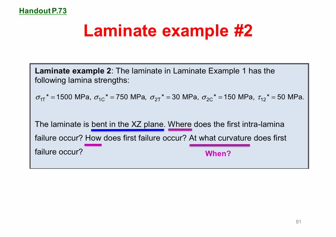
81

Laminate example 2: The laminate in Laminate Example 1 has the following lamina strengths:

1T 1C 2T 2C 12* 1500 MPa, * 750 MPa, * 30 MPa, * 150 MPa, * 50 MPa.σ σ σ σ τ= = = = =

The laminate is bent in the XZ plane. Where does the first intra-lamina

failure occur? How does first failure occur? At what curvature does first

failure occur?

Handout P.73

When?

Extras

82

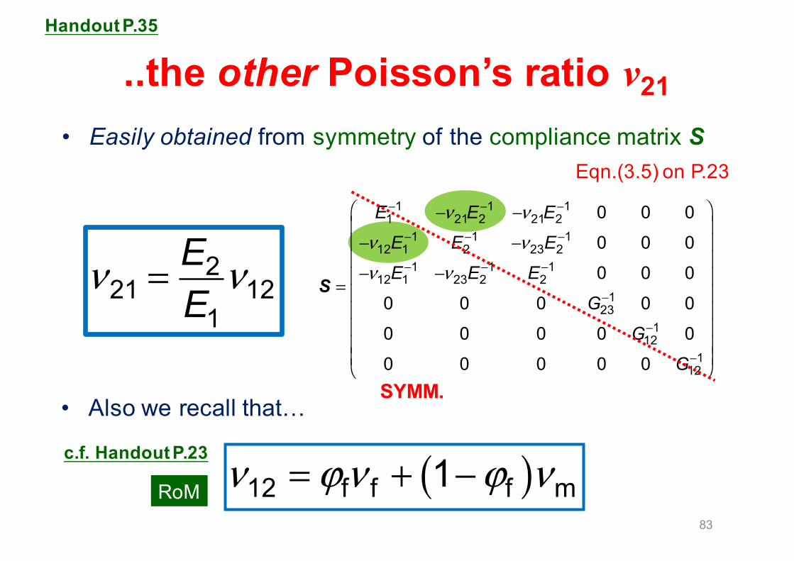
..the other Poisson’s ratio ν21

83

• Easily obtained from symmetry of the compliance matrix S

221 12

1

EE

ν ν=

• Also we recall that…

Handout P.35

( )12 f f f m1ν ϕ ν ϕ ν= + −c.f. Handout P.23

1 1 11 21 2 21 2

1 1 112 1 2 23 2

1 1 112 1 23 2 2

123

112

112

0 0 0

0 0 0

0 0 0

0 0 0 0 0

0 0 0 0 0

0 0 0 0 0

E E E

E E E

E E E

G

G

G

ν νν νν ν

− − −

− − −

− − −

−

−

−

⎛ ⎞− −⎜ ⎟− −⎜ ⎟

⎜ ⎟− −⎜ ⎟= ⎜ ⎟

⎜ ⎟⎜ ⎟⎜ ⎟⎜ ⎟⎝ ⎠

S

SYMM.

Eqn.(3.5) on P.23

RoM

The case of a symmetric laminate

84

Handout P.64

eZ

eX

Uniform extensionof each layer

Stress distribution )σ (XX z

Note: there is no bending moment!

In a symmetriclaminate, there is no couplingbetween uniform in-plane strains and bending moments

MirrorplaneMz