Compound filter using the circular harmonic expansion
M. T. Manry
A compound rotation-invariant filtering technique is developed which leads to sharp cross-correlation peaksfor desired targets while suppressing random noise and unwanted target correlations. The basic compoundfilter structure is a filter bank consisting of several circular harmonic filters. The output image moduli fromthe filter bank are weighted and summed to form the final output image. In the design procedure, the weightsare constrained so that the compound filter output has a peak value of 1 for the desired target. Measures ofrandom noise and deterministic noise due to correlations with unwanted targets are minimized with respect tothe weights. The SNR of the compound filter is, therefore, maximized. The weights constitute a realsolution to a classical least-squares problem and are, therefore, unique. Some limits to the performance of thetechnique are discussed. Examples illustrating the filter performance are given. Optical, digital, and hybridimplementations of the compound filter are possible. Extensions of this work are discussed.
1. Introduction
In conventional shift-invariant optical correlationsystems, a target of known size and orientation can bedetected equally well, no matter where it is located.There have been many attempts to design systemswhich are scale-and rotation-invariant as well. In thelast few years, Hsu et al." 2 have used the circularharmonic expansion (CHE) to develop a complex im-pulse response filter which is part of a rotation andshift-invariant target detection system. Hsu and Ar-senault3 along with Wu and Stark4 have developedmethods for utilizing several of these circular harmon-ic filters (CHFs) to improve performance. Schils andSweeney5'6 have shown that the linear combinationfilters of Caulfield et al. 7-' 3 can be formed as a cycliccorrelation of the image to be detected with a functionof rotation angle 0. They have also developed filterswhich are rotation-invariant for a limited range ofrotation angles.
Several problems remain. Individual CHFs oftenhave very poorly shaped autocorrelation functions andare not very useful for discrimination between classesof object, although they are rotation- and shift-invari-ant. In this paper a rotation-invariant filtering tech-nique is developed which leads to sharp cross-correla-tion peaks for desired targets, while suppressingrandom noise and unwanted target correlations. Thebasic filter structure is given in Sec. II. Measures of
The author is with University of Texas at Arlington, Departmentof Electrical Engineering, Arlington, Texas 76019.
Received 15 September 1986.0003-6935/87/173622-06$02.00/0.
noise and a constraint on the cross-correlation func-tions are introduced in Sec. III. A technique for maxi-mizing the SNR of the filtering approach is describedin Sec. IV. Some limits to the performance of thetechnique are also discussed. Examples are given inSec. V.
II. Filter Structures
A. Circular Harmonic Filters
Let f (r,O) denote a complex target image in polarcoordinates. f can be represented using the circularharmonic expansion as
f(r,O) = f(r) exp(mO),m=-X
where2,,
fm(r) = (1/27r) fJ f(r,O) exp(-jmO)dO.
Let hm (xy) represent a complex filter defined as
hm(x,y) = ,(r) exp(-jmO),
(1)
(2)
(3)
where (x,y) are the rectangular coordinates corre-sponding to (r,O) and where the origin in polar coordi-nates is located at (xy) = (xc,yc). This point is calledthe center of expansion. From Eqs. (1)-(3),
JJ hi(xy)ha(xy)dxdy = (i - k) JJ Ihi(xsy)I2 dxdy, (4)
where 5(n) is the Kronecker delta function. In theremainder of this paper, continuous functions of (xy)are represented by sampled versions with (x,y) takingon integer values in a set N1. Let f(xmy) represent therectangular coordinate version of the target imagef(r,O). The output from the discrete convolution f * hmis
It is known that as f(x,y) rotates about its center ofexpansion, so does Izm(x,y)I. The center of expansionis known as a proper center1 if the maximum oflZm(xy)I occurs at that location.
B. Problems With Circular Harmonic Filters
The circular harmonic filters, developed up to thepresent time, have many difficulties, as discussed inthe following.
Individual CHFs h sometimes lead to poorlyshaped cross-correlation peaks. Often the cross-cor-relation peak for the desired target will be less inamplitude than the cross-correlation peak for an un-wanted target or object. These problems may be rem-edied if several CHFs can be combined or used inparallel. However, it has been pointed out that alinear combination of two CHFs as hm(X,y) + h.(xy)leads to an output correlation with a peak which variessinusoidally as the input image is rotated.
To avoid this difficulty, Hsu and Arsenault,3 alongwith Wu and Stark,4 have used a feature vector com-posed of CHF cross-correlation magnitudes in targetclassification experiments. Feature vectors have diffi-culties also. First, it can be very difficult to find thecorrect center of expansion (xc,Yc) on the filtered out-put images zm(X,y). There is a second difficulty inusing the functions Izm(x,y)l for target detection andclassification. There exist an uncountable number ofreal deterministic functions f(x,y) having the samefeature vector [m(xcyc)l]m. In other words, the fea-ture vector is not unique.
C. Compound Circular Harmonic Filters
There are other methods of utilizing multiple har-monics. One can form a filter bank consisting of thefilters hm(x,y) and perform the weighted sum of themoduli of their outputs. The final filter bank output
Z(Xy) = > amlzm(xy)12, (6)mN2
where N2 is a finite set of non-negative integers withlargest member M. As the input f(x,y) rotates, z(xy)clearly rotates but does not change shape or amplitude.The coefficients am can be chosen so that z(x,y) has asharp peak for one input target image. Although theimplementations of this approach to date have beendiscrete computer implementations, it is possible torealize the technique optically or in a hybrid optical-digital system. In the remainder of this paper theoutput image z(x,y) is referred to as the compoundCHF output, and the filter bank is referred to as thecompound circular harmonic filter.
In general, the function z(x,y) can be unique, evenwhen the feature vector [zm(xcYc)l]m is not. If onecomponent of z(xy), z3(xy), for example, is rotated,the shape of z(xy) will change.
D. Coefficient Constraints
The basic goal is to force z(x,y) to have a sharp peakfor a specific target. The first step in accomplishingthis is to pick a point (xc,yc), where the peak is to belocated. This point is the center of expansion forf(x,y). The center of expansion is an estimate of thegroup proper center, which is formally defined in Sec.IV. The second step is to constrain z(x,y) at that pointas
z(x0,y,) = 1. (7)
The functions zm(x,y) are normalized so that lzm(xcYc)I= 1. This is done as
Cm = 1/lzm(Xcyc)l,
hm(x,y) hm(xy) Cm,
and recalculating zm(X,y) in Eq. (5) with the newhm(x,y) terms. Now, by letting the weights am satisfythe relation,
aM= 1 am, (8)mN3
Eq. (7) is satisfied. N3 denotes the set N2 minus theintegerM. The next steps are to define the noise of thecompound filter, to define a SNR, and to maximize theSNR with respect to the am terms. The noise includesthe cross-correlation energy outside the point (xcyc).Therefore, the spatial extent of the correlation func-tion z(x,y) is minimized when the SNR is maximized.
111. Measures of Noise
Before optimizing the compound filter's perfor-mance, it is necessary to develop measures for thenoise, which limits performance. There are three ba-sic types of noise to be quantified for the functionz(x,y). In this section measures for all three types ofnoise are developed. To save space, functions of x andy are occasionally written without the (x,y).
A. Deterministic Noise
A measure of the correlation noise in z outside thecorrelation peak is
Ed(a) = E z2(x,y).Nc
(9)
Here a is the vector of unknown weights(ai,a 2,. .. ,aM)', and Nc is Nt - Nc', where Nc' is arectangular neighborhood of dimensions (1 + 2Nx) by(1 + 2Ny) centered at the point of expansion. Theneighborhood Nc' is a transition region, where thecorrelation is allowed to change from its value of 1 at(xc,yc) to a small value in the set Nc. MinimizingEd(a) will sharpen the correlation peak and limit thespatial extent of z(xy). A second type of determinis-tic noise is the cross-correlation of the CHFs withunwanted targets. The noise in unwanted target cor-relations is measured as
and where gu(x,y) represents an unwanted target. IfEu(a) is now minimized with respect to the am terms,the compound filter should discriminate against un-wanted targets gu(x,y). Because of the nature of theCHE, only one orientation of each of these unwantedtargets is required.
B. Measure of Random Noise
The second type of noise affecting correlation sys-tems is random noise.14 To quantify this noise, zm canbe replaced141 6 as
zm(x,y) = hm(xy) * [f(xy) + e'(x,y)]
= Zm(xy) + em(x,y), (11)
z'(XY) = Zam[lzm(xy)j2 + nm(x,y)]N2
= z(x,y) + e(xy),
where
e(x,y) = >amnm(xy)N2
= amnm(xy) + (1 - z am)nM(X'Y)'N3 N3
nfm(xy) = lem(xy)12 + zm(xy)e,(xy)
+ 4m(xy)em(xy).
The final measure of random noise is then
Er(a) = I E[e2 (x,y)]
N1
= 11 aiaj> E(ninj).i j N1
An overall measure of the noise can be formed asEn(a) = b * Ed(a)/N + c Eu(a)/Nt
+ (1 - b - c) * Er(a)/Nt, (15)
where Nt and Nu are the numbers of elements in setsN1 and Nc, respectively. Thus the noise definitioncan be adjusted by changing the values of b and c. Ifthe filter designer principally wants to discriminateagainst unwanted targets, he can make c large withrespect to b. If a sharp correlation peak for the desiredtarget is his principal concern, he can choose b to beclose to 1.
IV. Signal-to-Noise Ratio
In this section, an SNR for the compound CHF isdefined and maximized with respect to the coefficientsam.
A. Definition and Maximization
The SNR can now be defined as SNR (a) = Z(xcyc)/En(a)0 5. Since z(xcyc) = 1 in Eq. (7),
(12)SNR(a) = 1/En(a) 0 i5 . (16)
For convenience, assume that N2 consists of the inte-gers from 1 to M. SNR(a) is then maximized by solv-ing the M - 1 equations in M - 1 unknowns represent-ed by the mth equation
(13)
(14)
The noise random process e'(x,y) is assumed station-ary with known probability density. Note that e(x,y)is signal-dependent and, therefore, nonstationary.Er(a) is a measure of noise in the vicinity of the cross-correlation function Zm. When e'(xy) has an evenprobability density,14
E(nink) = E(leiek1l) + ziz4E(e'ek) + Z.ZkE(eiek).
When e'(x,y) can be approximated as white, zero-meanGaussian noise with variance 2, the methods of Ref. 15can be used to show that
E(eieC) = A2l(i - k) I Ihi(tw)12
N1
E(leiel 2 ) = 4 Ihi(t,W)12 3 Ihk(nP)I2]
+ a46(k - i)[ Ihi(np) 12]Nl
aEn(a)/Oam = 0,
which can be rewritten asM-1
E A(m,k)-ak= B(m),k=l
(17)
(18a)
A(m,k) = b [ (Zk12 - IZMI)(IZm 2- IZMI)1
Nc
+ (N,/Nt)c E(IZuk 1N1
- ZUM)(Zum - IZUMI2)
+ (NJ/N)(1 - b - C) EE[(nk - nM)(nm -nm)]N1
(18b)
and B(m) can be calculated as
B(m) = b IZMI2(Zm12 - ZMI2)Nc
- (N,,INt)c I I Z"MI (lZuml2 IZUMI2)N1
- (Nl/N)(1 -b-c) 3 E[nM(nm - nM)].N1
(18c)
From Eqs. (17) and (18), the am terms are the solutionto a classical least-squares problem, such as those de-scribed in Ref. 16 and 17. Obviously, there exists oneunique real solution that minimizes the error En(a)and maximizes the SNR. The group proper center can
now be defined as that center of expansion (xc,yc) forwhich SNR(a) is maximum.
1ne n~ nt 3 W**_**#S}M&W
34 846*546USin-U 34
SSS ,1 _ .4& 4 1 . f
$54 N * 1 6 4 *S S . 44]
$*e *XSC'f S . 104O
314f . S**SS I&f U W tl34 . *f1ISSS SS , *V
SS . _ . >NSS~~~10
'SSI .'W~ioltF)O 44*5
B. Performance Considerations
Note that lzIm(X,Y)I21 is a nonorthogonal set of basisfunctions of x and y and that z(xy) is a linear combina-tion of the functions. The set contains M functions,each of which can be considered to be a vector havingNt elements. In theory M can be chosen to equal 1 +Nt. Then, the equations consisting of Eq. (8) plusEd(a) = 0 from (9), or Eq. (8) plus Eu(a) = 0 from (10),
or Eq. (8) plus Er(a) = 0 from Eq. (14) can be solvedexactly. Therefore, any one of the three componentsof En(a) can be driven to zero. This assumes that theset is linearly independent. However, the calculationof the CHE for such a large value of M is not practical.
It is important to consider the behavior of the errormeasures as functions of b, c, and the vector a.
Theoreml1: Let EdM, EuM, ErM, and nm representthe minima of Ed(a), Eu(a), Er(a), and En(a) withrespect to a. Then the sequences EdM}, EumI, ErM},and Enm}, all with index M, are nonincreasing.
This is a well-known property of least-squares ap-proximations.16 17 Therefore, increasing the numberof coefficients am decreases En(a), decreases Ed(a) if b= 1, decreases Eu (a) if c = 1, and decreases Er(a) if b =c = 0. The next theorem examines the effects of thevector a on Er(a).
Theorem 2: Suppose that b + c = 1 so that Er(a)receives no weight in Eq. 15. Then some choices of thevector a make Er(a) arbitrarily large.
Proof: Note that if a2 = (1 - a) and the othermembers of a are zero, Er(a) contains a positive num.-ber multiplied by al
In a real world situation, it is advisable to give non-zero weight to each component of En(a).
V. Examples
As an example consider the desired target f(xy)depicted in Fig. 1 and the unwanted target gu(x,y) ofFig. 2. The cross-correlation Iz2(x,y)12 and the finaloutput z(xy) for b = 0.9 and c = 0.1 are shown in Figs. 3and 4. The values of m were m = 2, 3, 5, 7, 8, and 9,
while Nx and Ny were both 5. From the SNR values ofTable I, it is clear that the compound filter performsbetter than any of the component filters. The quanti-ty SNR2 in the table is z(xC,yc) divided by the peakvalue of zu(x,y). Clearly, the three filters with thepoorest SNRs had negative weights a(m), while thefilter with the highest SNR got the largest weight.
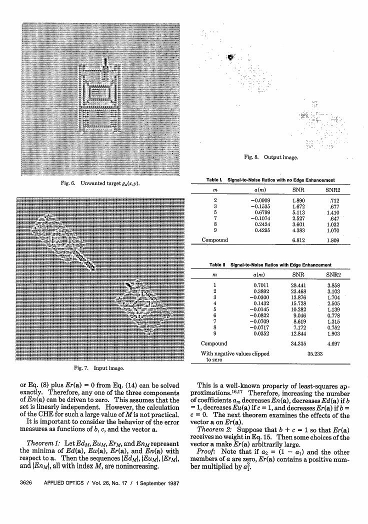
As a second example, consider the functions f(xy)and gu(x,y) in Figs. 5 and 6. These are the same asFigs. 2 and 1, respectively, after the application of a 3 X3 LaPlacian edge detector. The compound filter wasformed for b = 0.05 and c = 0.95, using m = 1-9 and Nx= Ny = 5. The resulting SNRs and a(m) terms aregiven in Table II. As in the previous example, thecomponent filters having the largest SNRs got thehighest weights. The method's improved perfor-mance in this example is due to the edge detection,which confirms the comments of Wu and Stark4 con-cerning the use of zero-mean images. In Table II,SNR(a) is recalculated using only the positive samplesof z(x,y) and zu(x,y). Contrary to expectations, thisled to a very slight increase in the SNR. The com-pound filter was applied to the input image of Fig. 7.The resulting output function z(xy) is shown in Fig. 8.The filter clearly has no trouble discriminating f(x,y)from gu(x,y).
For the examples in this paper, it is clear that theLaPlacian edge detector increases the SNR functionmore than the use of multiple components does. How-ever, in real-world situations LaPlacian filters can beexpected to boost the random noise component Er(a)substantially.
VI. Conclusions
A compound filter structure has been introducedwhich pmploys several CHFs, leading to a rotation-andshift-invariant cross-correlation function. Since themodulus of each CHF output is used, this structureshould be realizable with existing hardware. Mea-sures of the deterministic and random noise for thisstructure have been developed, and a method for maxi-mizing the SNR has been given. Examples have beengiven which illustrate the performance of the tech-nique.
Further work is possible. A reliable method is need-ed for finding the group proper center at which theSNR is highest. It may be possible to design CHFs sothat the compound structure introduced here can getby with a lower value of M. It will also be useful todefine and maximize SNRs other than the one present-ed here.
This work was performed at the Research Director-ate, U.S. Army Missile Command, Redstone Arsenal,Alabama, under a Scientific Services Agreement is-sued by Battelle Columbus Laboratories.
References
1. Y.-N. Hsu, H. H. Arsenault, and G. April, "Rotation-Invariant
Digital Pattern Recognition Using Circular Harmonic Expan-sion," Appl. Opt. 21, 4012 (1982).
2. Y.-N. Hsu and H. H. Arsenault, "Optical Pattern RecognitionUsing Circular Harmonic Expansion," Appl. Opt. 21, 4016
(1982).3. Y.-N. Hsu and H. H. Arsenault, "Pattern Discrimination by