SANDIA REPORT SAND2012-6965 Unlimited Release Printed September 2012 Compound Multi-Frame Radar Waveforms Armin W. Doerry, Brandeis Marquette Prepared by Sandia National Laboratories Albuquerque, New Mexico 87185 and Livermore, California 94550 Sandia National Laboratories is a multi-program laboratory managed and operated by Sandia Corporation, a wholly owned subsidiary of Lockheed Martin Corporation, for the U.S. Department of Energy's National Nuclear Security Administration under contract DE-AC04-94AL85000. Approved for public release; further dissemination unlimited.
Transcript
SANDIA REPORT SAND2012-6965 Unlimited Release Printed September 2012
Compound Multi-Frame Radar Waveforms
Armin W. Doerry, Brandeis Marquette
Prepared by Sandia National Laboratories Albuquerque, New Mexico 87185 and Livermore, California 94550
Sandia National Laboratories is a multi-program laboratory managed and operated by Sandia Corporation, a wholly owned subsidiary of Lockheed Martin Corporation, for the U.S. Department of Energy's National Nuclear Security Administration under contract DE-AC04-94AL85000.
Approved for public release; further dissemination unlimited.
- 2 -
Issued by Sandia National Laboratories, operated for the United States Department of Energy by Sandia Corporation.
NOTICE: This report was prepared as an account of work sponsored by an agency of the United States Government. Neither the United States Government, nor any agency thereof, nor any of their employees, nor any of their contractors, subcontractors, or their employees, make any warranty, express or implied, or assume any legal liability or responsibility for the accuracy, completeness, or usefulness of any information, apparatus, product, or process disclosed, or represent that its use would not infringe privately owned rights. Reference herein to any specific commercial product, process, or service by trade name, trademark, manufacturer, or otherwise, does not necessarily constitute or imply its endorsement, recommendation, or favoring by the United States Government, any agency thereof, or any of their contractors or subcontractors. The views and opinions expressed herein do not necessarily state or reflect those of the United States Government, any agency thereof, or any of their contractors.
Printed in the United States of America. This report has been reproduced directly from the best available copy.
Available to DOE and DOE contractors from
U.S. Department of Energy Office of Scientific and Technical Information P.O. Box 62 Oak Ridge, TN 37831 Telephone: (865) 576-8401 Facsimile: (865) 576-5728 E-Mail: [email protected] Online ordering: http://www.osti.gov/bridge
Available to the public from
U.S. Department of Commerce National Technical Information Service 5285 Port Royal Rd. Springfield, VA 22161 Telephone: (800) 553-6847 Facsimile: (703) 605-6900 E-Mail: [email protected] Online order: http://www.ntis.gov/help/ordermethods.asp?loc=7-4-0#online
- 3 -
SAND2012-6965 Unlimited Release
Printed September 2012
Compound Multi-Frame Radar Waveforms
Armin W. Doerry ISR Mission Engineering
Sandia National Laboratories Albuquerque, NM 87185-0519
Brandeis Marquette Reconnaissance Systems Group
General Atomics Aeronautical Systems, Inc. San Diego, CA 92127
Abstract
A radar pulse may be divided into multiple frames, where each frame can be independently modulated. Furthermore, echo signals can be processed against the individual frames. This allows overcoming traditional limits on the observable near range being constrained to the delay for the entire pulse.
- 4 -
Acknowledgements
The production of this report was funded by General Atomics Aeronautical Systems, Inc. (ASI) Reconnaissance Systems Group (RSG).
GA-ASI, an affiliate of privately-held General Atomics, is a leading manufacturer of unmanned aircraft systems (UAS), tactical reconnaissance radars, and surveillance systems, including the Predator UAS series and Lynx Multi-Mode radar systems.
3.1 Dividing a Pulse Into Independent Frames ........................................................ 13 3.2 Selecting Frame Widths ..................................................................................... 17
3.2.1 Single Frame ............................................................................................... 17 3.2.2 Two Frames ................................................................................................ 17 3.2.3 Arbitrary Number of Frames ...................................................................... 19
Processing ................................................................................................ 52 3.4.2.2 Basic LFM Chirp Frames Spectrally Separated with Random Reference
Phase and Windowed Processing ............................................................ 56 3.4.2.3 Shuffled Frequency Hops Spectrally Separated with Random Reference
Phase and Windowed Processing ............................................................ 60 3.5 Comments........................................................................................................... 64
4 Conclusions ............................................................................................................... 65 Appendix A – Details of 50 dB Taylor Window (nbar = 7) ........................................... 67 References ......................................................................................................................... 69 Distribution ....................................................................................................................... 70
- 6 -
Foreword
General Atomics Aeronautical Systems, Inc., builds the high-performance Lynx SAR/GMTI system.
This report details the results of an academic study. It does not presently exemplify any modes, methodologies, or techniques employed by any operational system known to the authors.
The specific mathematics and algorithms presented herein do not bear any release restrictions or distribution limitations.
This distribution limitations of this report are in accordance with the classification guidance detailed in the memorandum “Classification Guidance Recommendations for Sandia Radar Testbed Research and Development”, DRAFT memorandum from Brett Remund (Deputy Director, RF Remote Sensing Systems, Electronic Systems Center) to Randy Bell (US Department of Energy, NA-22), February 23, 2004. Sandia has adopted this guidance where otherwise none has been given.
This report formalizes preexisting informal notes and other documentation on the subject matter herein.
- 7 -
1 Introduction & Background
A typical pulse-Doppler radar system emits a series of pulses, and collects echo signals. For each pulse, these echo signals are correlated against the transmitted waveform to provide a range sounding, and the range soundings are compared against each other across pulses to discern Doppler information. The correlation function may be implemented as an equivalent matched filter, or as a direct correlation.
Typical radar modes that operate in this fashion include Synthetic Aperture Radar (SAR), Inverse-SAR (ISAR), various Moving Target Indicator (MTI) radars, and coherent search radar systems. This is certainly not an exhaustive list. Herein we concern ourselves with generically range-Doppler radars.
The choice of waveforms to use will depend on the objectives of the radar system with respect to ease of generation, downstream processing issues, and desires for probabilities of detection, interception, spoofing, etc. We typically desire waveforms that offer a large time-bandwidth product to afford both high energy and wide bandwidth for improved range resolution. There are a plethora of waveforms from which to choose. These would include, but are not limited to, the popular Linear-Frequency-Modulated (LFM) chirp, Non-Linear FM (NLFM) chirp, stepped frequency systems, various phase-coded modulation schemes, and even random and pseudo-random noise waveforms. Each has its own set of advantages and disadvantages.
It is well-known that the output of a matched filter, when input with a signal to which it is matched, is the autocorrelation function of the waveform. Furthermore, the autocorrelation of a function is related by the Fourier Transform (FT) to the Energy Spectral Density (ESD) of the waveform. That is, the autocorrelation function and ESD are FT-pairs. We desire matched filters as their principal advantage is to maximize the Signal-to-Noise Ratio (SNR) of energy in the final range-Doppler map. Most radar processing seeks to implement matched filters, or at least nearly so.
The choice of pulse width for pulsed radar systems is necessarily a compromise in performance. We desire long pulses to increase the energy in the signal to afford larger SNR, especially at longer ranges. Many radar systems are limited in their range performance by achievable SNR. However, we desire short pulses to facilitate near-range operation. Essentially, the radar must end its transmitted pulse and switch to a receive mode before the echo from a near range target returns to the radar. Modern radar systems typically address this trade by interleaving data collections at longer ranges with data collections at shorter ranges. When the interleaving is on a scan-to-scan basis, the individual range-dependent configurations are sometimes called “scan bars”. We desire a mechanism whereby we get the benefits of a long pulse along with the benefits of a short pulse, all in a single pulse.
To be sure, some echo energy from near-range targets is present even when a long pulse is used. Although perhaps most of the near range target echo is occluded or eclipsed by the continued transmission of the latter portion of a long pulse, some portion of the pulse
- 8 -
near the trailing edge of the pulse will in fact be present in the echo data after the pulse’s transmission ceases. The problem with this is that the partial echo does not contain the entire modulation of the entire pulse. For most typical modulation schemes this means that significant parts of the pulse’s spectrum is missing in the data, resulting in substantially impacted resolution (i.e. impacted not in a good way).
In this report we describe a new modulation scheme that creates a compound pulse that allows a single pulse to overcome the limitations described above. The compound pulse will allow long pulses with desired resolution bandwidth for long range performance, and short-range performance with desired resolution bandwidth that tolerates received echo partial occlusion.
Towards this end, we present the following reference material as background information.
Several papers mention “compound” waveforms, but apply this term to spread-spectrum modulation schemes such as Barker codes for bi-phase modulation. Examples of such papers include Petrovic, et al.1
Kalenichenko & Mikhailov2 use the term “compound waveform” to describe a modulation scheme that may be used for radar as well as communication. They describe doing so by using sequences of up-chirps and down-chirps.
Benjamin3 uses the phrase “a single long pulse that is built up of n contiguous short pulses”, but uses this to refer to phase modulation where his “short pulses” are really waveform ‘chips’ with different reference phase.
Ziomek & Jones4 discuss a waveform generator for Automated Test Equipment (ATE) applications that offers the ability to “to piece together standard or arbitrary waveforms in stages to create a user defined compound waveform”. Radar applications are not specifically addressed.
Li, et al.,5 propose adjusting waveform parameters from dwell to dwell to optimize target detection. All pulses within a dwell are identical waveforms.
Dawber & Nichols6 discuss the problem of “eclipsing” received echo signals that overlap the transmitted waveform. Their concern is the high processing sidelobes due to the incomplete range returns. They propose to process the data in a manner to reduce sidelobes of eclipsed targets, which would come at the expense of other waveform performance parameters.
A concept for using sequential independent pulses of different widths to interrogate different ranges is presented by Harman.7
A paper by Krieger, et al.,8 presents what they term “Multidimensional Waveform Encoding” which divides a pulse into sub-pulses, in particular for orbital radar
- 9 -
applications. Their discussion includes allowing sub-pulses to be beam-steered independently to facilitate range-dependent returns that can be combined in a Digital Beam-Forming (DBF) fashion.
A discussion of random-phase waveforms with shaped spectra is given in a Sandia report by Doerry & Marquette.9 Within this report can be found references to other publications relevant to noise waveforms.
Techniques for designing, producing, and processing Non-Linear FM chirp waveforms are presented in a pair of Sandia reports by Doerry.10,11
In this report, we detail and build on pulse segmentation and modulation concepts like those reported by Krieger, et al.
- 10 -
“In order to be irreplaceable one must always be different.” -- Coco Chanel
- 11 -
2 Overview & Summary
We begin by noting that most pulse modulation schemes make the assumption that the receiver’s matched filter will process substantially the entire pulse to generate an output with the desired characteristics, typically measured with the radar’s Impulse Response (IPR).
A pulse may be divided into contiguous sequential frames, sometimes called sub-pulses.
In a typical pulse-Doppler radar, receiving echo energy must be deferred until after the entire pulse waveform is transmitted. This sets a nearest possible range at which the beginning of the echo pulse can be processed.
However, even when early frames or portions of frames are occluded or eclipsed by the transmit pulse, the echo from later frames may still be received and processed. This allows latter frames to be received in their entirety from nearer ranges than earlier frames or the entire pulse.
As long as the latter frames still exhibit the desired resolution bandwidth, no loss of resolution is suffered by processing against only the latter frames.
In this manner, a compound multi-frame pulse can be processed against a larger range swath than a more conventional pulse modulation scheme. Essentially, the traditional constraints between near-range detection and pulsewidth have been considerably loosened.
Relative frame durations can be optimized to allow SNR to exceed some minimum level.
- 12 -
“Coming together is a beginning. Keeping together is progress. Working together is success.”
-- Henry Ford
- 13 -
3 Detailed Analysis
The measure of a pulse modulation scheme is the autocorrelation function. The autocorrelation function is simply a cross-correlation of a function with itself.
The goal herein is to design a modulation scheme for a pulse that facilitates the following.
1. Long range performance by allowing an acceptable autocorrelation function for substantially the entire pulse.
2. Short range performance by allowing an acceptable cross-correlation of a portion of the entire pulse with an occluded, or partially masked, version of the entire pulse.
To meet this compound set of requirements, we propose a compound multi-frame waveform. We define a compound multi-frame waveform as one that is composed of components that by themselves have attributes of independent waveforms.
3.1 Dividing a Pulse Into Independent Frames
Our general approach to the new compound waveform is to divide the waveform into frames. More specifically, we design the structure as follows.
1. Each pulse is divided into two or more contiguous frames.
2. Each frame is essentially a separate waveform, with individual characteristics.
3. Each frame is designed to not correlate well with any other frame. This property is often referred to as orthogonality.
We illustrate this in Figure 1.
Fram
e 1
…
Pulse n Pulse n+1
Fram
e 2
Fram
e M
Fram
e 1
…
Fram
e 2
Fram
e M
Figure 1. Pulses may be divided into multiple frames, with each frame exhibiting different modulation characteristics.
- 14 -
We stipulate that individual frames do not necessarily need to be of equal length or duration, equal bandwidth, or even spectral content or characteristics. Separate pulses need not necessarily even be divided into equal, or even similar frames, in number or characteristics.
We will nevertheless continue with the following assumptions.
1. Each pulse will have the same number of frames.
2. Across pulses, i.e. from one pulse to the next, a particular frame will have the same length.
3. Within a pulse, different frames need not have the same length.
4. Modulation within a pulse for all frames will be phase/frequency, to facilitate radar power amplifiers operating in compression for maximum power output.
5. The pulse waveform will be digitally generated samples, to facilitate maximum control over pulse characteristics.
We define the notation for generic pulse as
nijT
iTAniP s ,exprect,
, (1)
where
A = amplitude of the pulse, i = intra-pulse index, 22 IiI , n = inter-pulse index, 22 NnN ,
sT = sample spacing within pulse,
ITT s = total pulse duration, (2)
and the phase and envelope functions are defined as
ni, = phase of the ith sample of the nth pulse, and
else
zz
0
211rect . (3)
We also define the basic pulse sample frequency as
ss T
f1
= sample frequency. (4)
- 15 -
We divide the pulse into frames by dividing the index i into frames via
22
1
1
IKkKi d
d
dd
, (5)
where
d = frame number within a pulse, Dd 1 ,
dK = duration in samples of the dth frame,
k = intra-frame sample index, 22 dd KkK . (6)
We stipulate that the frame index d increases with time within a pulse.
Each index i corresponds to a unique combination of indices k and d. In fact, we may calculate the individual unique component indices as
d = smallest d that satisfies
21
IiK
d
dd , and
1
122
d
dd
d KKI
ik . (7)
Furthermore, we observe that the sum of the lengths of the individual frames equals the total length of the pulse, that is
IKD
dd
1
. (8)
Given that we can parse the overall index i into new indices d and k, we can now speak in terms of individual frame modulations, that is
ndk ,, = the phase of the kth sample of the dth frame in the nth pulse. (9)
This allows us to develop modulation functions that are independent for each frame.
With malice of forethought, we will define the phase function as an accumulation of frequencies. That is, for each frame we allow
k
Kknd
d
ndkndk2
, ,,,, , (10)
where
- 16 -
nd , = reference phase for the dth frame in the nth pulse, and
ndk ,, = phase-rate per sample of the kth sample, dth frame, and nth pulse. (11)
The overall phase function is then
i
Iind ndkni
2, ,,, , (12)
where
22
1
1
IKkKi d
d
dd
. (13)
We have allowed the reference phase nd , to change with frame index d. This will
generally cause a phase discontinuity at frame boundaries where nd , changes. While
varying nd , may be useful, particularly in providing some orthogonality in Doppler
space, it does come at a price.
For convenience, we define the time duration of individual frames as
sdd TKT . (14)
We reiterate that we would normally desire that the waveform segments in individual frames to not correlate well with each other, as this would cause enhanced undesirable sidelobes in the overall waveform autocorrelation function. Furthermore, this works better with longer pulses to mitigate quantization effects in both time duration and frequency.
- 17 -
3.2 Selecting Frame Widths
3.2.1 Single Frame
In a typical pulse radar, with but a single frame, we desire the data we collect to contain the complete radar echo from a target of the entire pulse that is transmitted. We also desire to use as long a pulse as possible. For a particular desired near range, this means that we insist that the pulsewidth be no more than the round-trip echo delay time from the nearest range of interest. We state this as
nearRc
T2
, (15)
where
c = velocity of propagation of the radar wave,
nearR = near range of interest. (16)
If the pulsewidth were given, then this could be rearranged to
Tc
Rnear 2 . (17)
We are ignoring any switching times or other margins that a normally a part of a real radar design. We also note that for some radar system operating modes, notably those that employ LFM chirp waveforms with stretch processing, this may not be strictly true. However for typical stretch processing it is ‘nearly’ true, but comes at a price of some lost SNR. For our purposes, we will assume more general waveforms using correlation processing or matched filter processing. For a single-frame radar pulse, we will insist that this relationship holds.
3.2.2 Two Frames
Now consider a radar waveform with two frames. We index these as
2,1d . (18)
If we consider the entire pulse, then it remains true that
212:1, 22KKT
cT
cR snear . (19)
However, if we concern ourselves with only the second frame, then we may calculate a different near range, namely
- 18 -
22, 2KT
cR snear . (20)
Clearly, the two near ranges are different, and related as
2:1,2, nearnear RR . (21)
Very clearly, the echo from the final frame of the pulse will be received in its entirety from much nearer ranges than the range for the complete echo from the entire pulse. This is illustrated in Figure 2.
Fram
e 1
Pulse n
Fram
e 2
Echo interval
Minimum range delay for Frame 2
Minimum range delay for entire pulse
t
Figure 2. Timing diagram for pulse transmission and reception.
This might be exploited such that, for ranges nearer than that 2:1,nearR which receives
the entire pulse, we can still receive the complete final frame down to the closer range
2,nearR . However, to maintain range resolution down to 2,nearR , we would need to
ensure that the spectral characteristics of Frame 2 are equal to that of the entire pulse.
Furthermore, we only need to consider the individual Frame 2 at ranges less than
2:1,nearR . This means that the far range to be considered for just Frame 2 is equal to the
near range for the entire pulse, namely
2:1,2, nearfar RR . (22)
Ostensibly there is also a far range of interest for the entire pulse as well. Consequently we may order the various ranges as
2:1,2:1,2,2, farnearfarnear RRRR . (23)
The far range for any one pulse is usually chosen based on SNR concerns. Neglecting antenna beam effects and atmospheric effects, for a single pulse, SNR of the echo signal
- 19 -
varies as the inverse of the fourth power of range, but linearly with pulse width. Consequently, if we desire SNR at 2,farR using only Frame 2 to be no less than to the
SNR at 2:1,farR using both frames, then we may relate
4
2:1,
214
2,
2
farfar R
KK
R
K . (24)
This may be transmogrified to the relationship
4
2:1,
521
4
22
far
s
R
KKTc
K
. (25)
This says that once the far range is chosen in conjunction with a total pulsewidth, then an optimum frame width may be calculated so as to not lose SNR at nearer ranges than the classical limit.
Effectively, the near range has been reduced to
4
2:1,
2:1,
21
2
2:1,
2,
far
near
near
near
R
R
KK
K
R
R. (26)
For example, if far range was desired to be 100 km, but the pulse width required to do this limited near range to be 70 km, then by employing a compound pulse with 2 frames, and optimally selecting the frame widths, we could reduce near range due to Frame 2’s lesser width to 24 km. Recall however that this ignores atmospheric propagation effects and antenna beam roll-off. Nevertheless, this is a significant improvement.
3.2.3 Arbitrary Number of Frames
Now consider a radar waveform with an arbitrary number of frames. We index these in temporal order (earlier to later) as
Dd ,...,2,1 . (27)
If we consider the entire pulse, then it remains true that
D
ddsDnear KT
cT
cR
1:1, 22
. (28)
However, if we concern ourselves with only a subset number of frames that are nearest to the final edge, then we may calculate a different near range for this subset, namely
- 20 -
D
dddsDdnear KT
cR
2:, . (29)
Clearly, two near ranges are different for different subsets, and related as
DdnearDdnear RR :,:, 12 if 21 dd . (30)
Very clearly, the echo from later frames of the pulse will be received in their entirety from much nearer ranges than the range for a more complete set of frames.
Following the logic from the analysis of only 2 frames, we insist that far ranges for a set of frames is equal to the near range for the same set of frames plus one earlier frame.
Consequently we may order the various ranges consistent with the rule
DdfarDdnearDdfarDdnear RRRR :1,:1,:,:, . (31)
Relative frame sizes may be selected based on the same criteria for 2 frames discussed above, namely
4
:1,
14
:, Ddfar
D
ddd
Ddfar
D
ddd
R
K
R
K
. (32)
This may be transmogrified to the relationship
D
ddd
Ddfar
DdfarD
ddd K
R
RK
4
:,
:1,
1
. (33)
This says that once the far range is chosen in conjunction with a total pulsewidth, where 1d , then an optimum frame width may be calculated for the case 2d , so as to not
lose SNR at nearer ranges than the classical limit. This may be iterated for 3d
and so on, until Dd .
Effectively, the near range has been reduced at each stage by
4
:,
:,1
:,
:1,
Ddfar
DdnearD
ddd
D
ddd
Ddnear
Ddnear
R
R
K
K
R
R. (34)
- 21 -
We recall that
DdnearDdfar RR :,:1, . (35)
Consequently, these may be combined to the iterative calculation
4
:,
:1,
:1,
:2,
Ddnear
Ddnear
Ddnear
Ddnear
R
R
R
R, (36)
where we identify
DfarDnear RR :1,:0, . (37)
These may all be combined to the rule
1
1
4
:1,
:1,
:1,
:,
d
d
d
Dfar
Dnear
Dnear
Ddnear
R
R
R
R. (38)
The nature of the exponent causes near range for increasing number of frames to reduce very quickly.
For the previous example, where if far range was desired to be 100 km, but the pulse width required to do this limited near range to be 70 km, then by employing a compound pulse with 3 frames, and optimally selecting the different frame widths for minimum acceptable SNR, we could reduce near range due to the various frames’ lesser widths to less than 1 km. Recall again however that this ignores atmospheric propagation effects and antenna beam roll-off. Nevertheless, this is an accelerating improvement over the 24 km from the previous example with just 2 frames.
- 22 -
3.3 Evaluating Compound Multi-Frame Waveforms
The general intent is to process different range bands against different sets of frames within the compound waveform.
To facilitate further analysis, we identify a mask function as follows
else
dwithassociatediforiMd 0
1. (39)
Recall that
22
1
1
IKkKi d
d
dd
. (40)
Note that different masks are orthogonal, that is
021
iMiM dd for 21 dd . (41)
Furthermore, the masks are complete, that is
11
D
dd iM for all i. (42)
For convenience, we will define compound masks as sums of individual contiguous masks as
2
1
21:
d
ddddd iMiM . (43)
We recall that the output of a matched filter, when input with a signal to which it is matched, is the autocorrelation function of the desired signal, or waveform. Consequently the autocorrelation function becomes the tool for evaluating the ‘goodness’ of a waveform. Recall that the autocorrelation function for the nth pulse is defined as
nmiPniPmRI
Iin ,, *
12
2
. (44)
The asterisk ‘*’ superscript denoted complex conjugation.
- 23 -
For our multi-frame processing strategy, we must modify this somewhat. The tool we will employ is the cross-correlation of the entire waveform with the particular set of frames we are considering for a particular range band. We calculate the appropriate cross-correlation function for the nth pulse of the entire waveform with reference frames
21 :dd as
nmiPiMniPddmC dd
I
Iin ,,:, *
:
12
221 21
. (45)
In some cases, we may be more interested in the results of multi-pulse processing, in which case our tool is the average of all cross-correlations over all pulses for a particular set of frames. Our calculation is then an expected value, namely
2121 :,:, ddmCEddmC nnavg . (46)
This is particularly true when at least some degree of randomness exists within a waveform.
- 24 -
“The whole is more than the sum of its parts.” -- Aristotle
- 25 -
3.4 Some Compound Multi-Frame Waveform Examples
There are a multitude of variations in how to employ multiple frames of a compound waveform. We discuss some examples here.
3.4.1 Shared Spectrum Frames
For this class of waveforms, our processing strategy is as follows.
1. Process the farthest ranges using as reference frames {1:D}.
2. Process the next nearest set of ranges using as reference frames {2:D}.
3. Process ever nearer sets of ranges using as reference ever fewer of the latest frames.
We will also presume the following characteristics of the individual frames.
Different frames will have different durations.
All frames will have substantially the same spectral width and shape, to offer substantially the same range resolution.
For the following examples, we will unless otherwise noted presume the following parameters.
sf 1 GHz = sample frequency,
T 160 s = overall total pulsewidth, 0f 500 MHz = pulse nominal center frequency,
TB 10 MHz = spectral bandwidth of frame, N = 128 pulses. (47)
Furthermore, we will presume a frame topology with
We consider here the example of a pulse with the aforementioned default parameters, but with each frame exhibiting the following additional features.
Both frames have positive chirps.
No window tapering is used in processing.
All pulses have identical reference phases for all frames.
Figure 3 details the instantaneous frequency of a pulse over the sample index. Frames are identified by color.
Figure 4 details the spectrum of the constituent components of the pulse. Note that the shorter frame contains less energy than the longer frame.
Figure 5 details the results of cross-correlating the constituent frames of the pulse with the entire pulse. Figure 6 is a zoomed rendering of this.
Figure 7 shows range-Doppler maps of the entire pulse echo signals after processing against constituent frames.
We observe in the cross-correlation plots that near-in sidelobes display a sinc ( xx sin ) characteristic. All cross-correlation products exhibit elevated far-out sidelobes. This is due to the individual frames interfering with each other. Note that cross-correlating with shorter frames yields higher far-out sidelobes.
- 27 -
-80 -60 -40 -20 0 20 40 60 80490
492
494
496
498
500
502
504
506
508
510
sample index (x1000)
freq
uenc
y -
MH
z
instantaneous frequency
Frame 1
Frame 2
Figure 3. Basic LMF chirps: Plot of instantaneous frequency vs. pulse sample index.
490 492 494 496 498 500 502 504 506 508 5100
10
20
30
40
50
60
70
80
90
100
mag
nitu
de -
dB
pulse/frame spectrum
frequency - MHz
total pulse
Frame 1Frame 2
Figure 4. Basic LMF chirps: Plot of spectrums of pulse frames.
- 28 -
-150 -100 -50 0 50 100 150
-60
-40
-20
0
dB
cross-correlation magnitude
total pulse
-150 -100 -50 0 50 100 150
-60
-40
-20
0
dB
Frame 1
-150 -100 -50 0 50 100 150
-60
-40
-20
0
dB
Frame 2
delay - samples (x1000)
Figure 5. Basic LMF chirps: Plots of cross-correlation of pulse segments with entire pulse.
-2000 -1500 -1000 -500 0 500 1000 1500 2000
-60
-40
-20
0
dB
cross-correlation magnitude - zoomed
total pulse
-2000 -1500 -1000 -500 0 500 1000 1500 2000
-60
-40
-20
0
dB
Frame 1
-2000 -1500 -1000 -500 0 500 1000 1500 2000
-60
-40
-20
0
dB
Frame 2
delay - samples
Figure 6. Basic LMF chirps: Zoomed rendering of previous plot.
- 29 -
total pulse
-60 -30 0
Frame 1
-60 -30 0
Frame 2
-60 -30 0
Figure 7. Basic LMF chirps: Result of Doppler processing of all pulses after respective cross-correlation operations against constituent frames. Colorbar values are dBc.
- 30 -
3.4.1.2 Counter LFM chirp frames
We consider here the example of a pulse with the aforementioned default parameters, but with each frame exhibiting the following additional features.
Each frame has the opposite chirp direction from the other.
No window tapering is used in processing.
All pulses have identical reference phases for all frames.
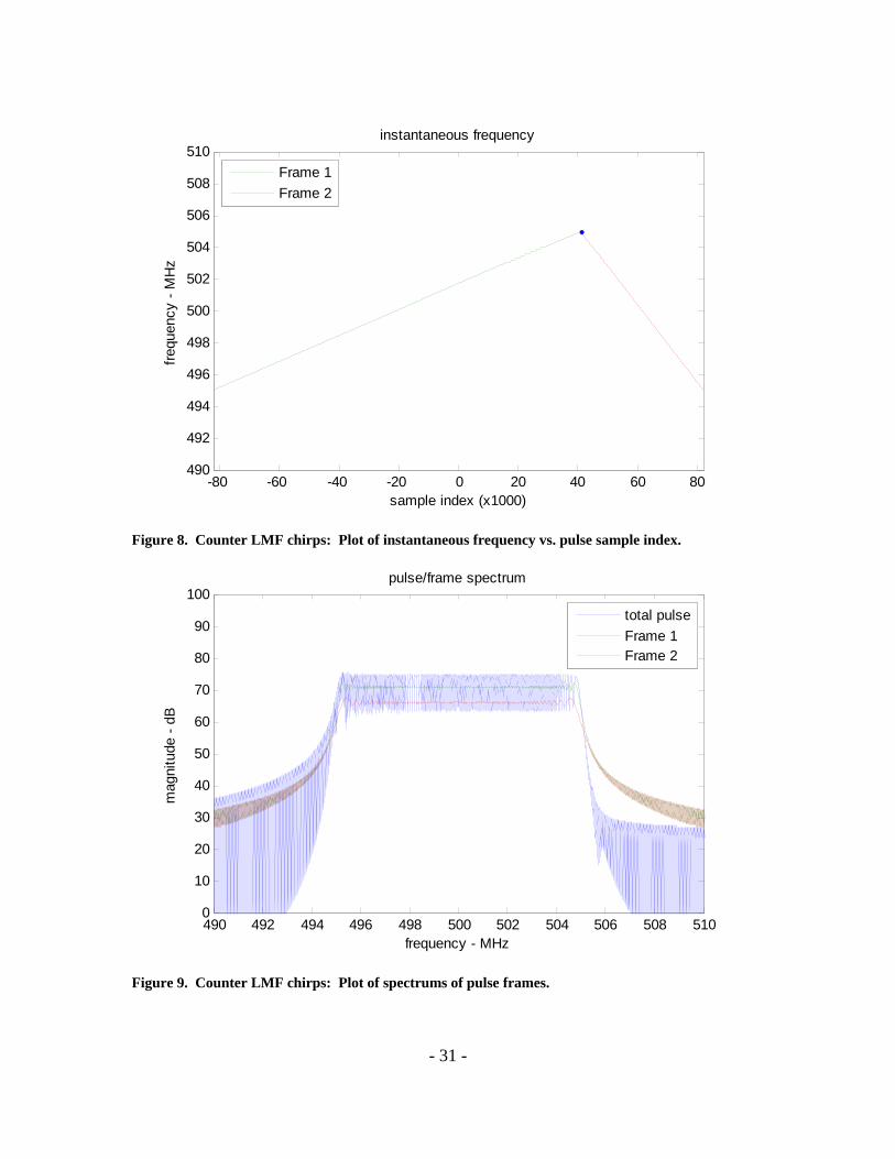
Figure 8 details the instantaneous frequency of a pulse over the sample index. Frames are identified by color.
Figure 9 details the spectrum of the constituent components of the pulse. Note that the shorter frame contains less energy than the longer frame.
Figure 10 details the results of cross-correlating the constituent frames of the pulse with the entire pulse. Figure 11 is a zoomed rendering of this.
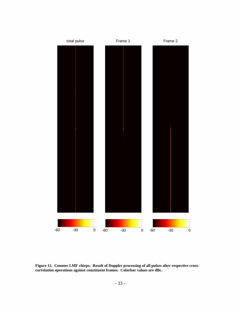
Figure 12 shows range-Doppler maps of the entire pulse echo signals after processing against constituent frames.
We observe in the cross-correlation plots that near-in sidelobes still exhibit a sinc characteristic. All cross-correlation products also still exhibit elevated far-out sidelobes. However, the counter-chirps cause these far-out sidelobes to spread even further, and thereby diminish in peak value.
- 31 -
-80 -60 -40 -20 0 20 40 60 80490
492
494
496
498
500
502
504
506
508
510
sample index (x1000)
freq
uenc
y -
MH
z
instantaneous frequency
Frame 1
Frame 2
Figure 8. Counter LMF chirps: Plot of instantaneous frequency vs. pulse sample index.
490 492 494 496 498 500 502 504 506 508 5100
10
20
30
40
50
60
70
80
90
100
mag
nitu
de -
dB
pulse/frame spectrum
frequency - MHz
total pulse
Frame 1Frame 2
Figure 9. Counter LMF chirps: Plot of spectrums of pulse frames.
- 32 -
-150 -100 -50 0 50 100 150
-60
-40
-20
0
dB
cross-correlation magnitude
total pulse
-150 -100 -50 0 50 100 150
-60
-40
-20
0
dB
Frame 1
-150 -100 -50 0 50 100 150
-60
-40
-20
0
dB
Frame 2
delay - samples (x1000)
Figure 10. Counter LMF chirps: Plots of cross-correlation of pulse segments with entire pulse.
-2000 -1500 -1000 -500 0 500 1000 1500 2000
-60
-40
-20
0
dB
cross-correlation magnitude - zoomed
total pulse
-2000 -1500 -1000 -500 0 500 1000 1500 2000
-60
-40
-20
0
dB
Frame 1
-2000 -1500 -1000 -500 0 500 1000 1500 2000
-60
-40
-20
0
dB
Frame 2
delay - samples
Figure 11. Counter LMF chirps: Zoomed rendering of previous plot.
- 33 -
total pulse
-60 -30 0
Frame 1
-60 -30 0
Frame 2
-60 -30 0
Figure 12. Counter LMF chirps: Result of Doppler processing of all pulses after respective cross-correlation operations against constituent frames. Colorbar values are dBc.
- 34 -
3.4.1.3 Counter LFM chirp frames with Random Reference Phase
We consider here the example of a pulse with the aforementioned default parameters, but with each frame exhibiting the following additional features.
Each frame has the opposite chirp direction from the other.
No window tapering is used in processing.
All pulses have independent random (uniformly distributed) reference phases for all frames.
Figure 13 details the instantaneous frequency of a pulse over the sample index. Frames are identified by color.
Figure 14 details the spectrum of the constituent components of the pulse. Note that the shorter frame contains less energy than the longer frame.
Figure 15 details the results of cross-correlating the constituent frames of the pulse with the entire pulse. Figure 16 is a zoomed rendering of this.
Figure 17 shows range-Doppler maps of the entire pulse echo signals after processing against constituent frames.
We observe in the cross-correlation plots that near-in sidelobes still exhibit a sinc characteristic. All cross-correlation products also still exhibit elevated far-out sidelobes. However, the randomized references phases cause these far-out sidelobes to spread in Doppler, and thereby diminishing in peak value. The 128 pulses cause the far-out range sidelobe average levels to diminish by slightly more than 20 dB in the same Doppler bin in this example. However, the random nature of the reference phases does not guarantee that the energy in any or all other Doppler bins will not exceed this. These levels will fluctuate.
- 35 -
-80 -60 -40 -20 0 20 40 60 80490
492
494
496
498
500
502
504
506
508
510
sample index (x1000)
freq
uenc
y -
MH
z
instantaneous frequency
Frame 1
Frame 2
Figure 13. Counter LMF chirps with random reference phase: Plot of instantaneous frequency vs. pulse sample index.
490 492 494 496 498 500 502 504 506 508 5100
10
20
30
40
50
60
70
80
90
100
mag
nitu
de -
dB
pulse/frame spectrum
frequency - MHz
total pulse
Frame 1Frame 2
Figure 14. Counter LMF chirps with random reference phase: Plot of spectrums of pulse frames.
- 36 -
-150 -100 -50 0 50 100 150
-60
-40
-20
0
dB
cross-correlation magnitude
total pulse
-150 -100 -50 0 50 100 150
-60
-40
-20
0
dB
Frame 1
-150 -100 -50 0 50 100 150
-60
-40
-20
0
dB
Frame 2
delay - samples (x1000)
Figure 15. Counter LMF chirps with random reference phase: Plots of cross-correlation of pulse segments with entire pulse.
-2000 -1500 -1000 -500 0 500 1000 1500 2000
-60
-40
-20
0
dB
cross-correlation magnitude - zoomed
total pulse
-2000 -1500 -1000 -500 0 500 1000 1500 2000
-60
-40
-20
0
dB
Frame 1
-2000 -1500 -1000 -500 0 500 1000 1500 2000
-60
-40
-20
0
dB
Frame 2
delay - samples
Figure 16. Counter LMF chirps with random reference phase: Zoomed rendering of previous plot.
- 37 -
total pulse
-60 -30 0
Frame 1
-60 -30 0
Frame 2
-60 -30 0
Figure 17. Counter LMF chirps with random reference phase: Result of Doppler processing of all pulses after respective cross-correlation operations against constituent frames. Colorbar values are dBc.
- 38 -
3.4.1.4 Counter LFM chirp frames with Random Reference Phase and Windowed Processing
We consider here the example of a pulse with the aforementioned default parameters, but with each frame exhibiting the following additional features.
Each frame has the opposite chirp direction from the other.
Cross-correlation processing will now employ a window taper function for sidelobe filtering. Specifically, we will employ a 50 dB Taylor window with
7n . The same window taper is used in azimuth Doppler processing.
All pulses have independent random (uniformly distributed) reference phases for all frames.
Figure 18 details the instantaneous frequency of a pulse over the sample index. Frames are identified by color.
Figure 19 details the spectrum of the constituent components of the pulse. Note that the shorter frame contains less energy than the longer frame.
Figure 20 details the results of cross-correlating the constituent frames of the pulse with the entire pulse. Figure 21 is a zoomed rendering of this.
Figure 22 shows range-Doppler maps of the entire pulse echo signals after processing against constituent frames.
We observe in the cross-correlation plots that near-in sidelobes now exhibit a Taylor window IPR. All cross-correlation products also still exhibit elevated far-out sidelobes, spread in Doppler due to the random reference phase. However, the window function causes the far-out processing sidelobes to ‘mound’ somewhat with a slight increase in the center of the mound. These mounds or ‘wings’ are in fact processing sidelobes that are a result of the windowing and cross-correlation function. The fact that they are not symmetric in the frame plots is because of interference between the frames.
- 39 -
-80 -60 -40 -20 0 20 40 60 80490
492
494
496
498
500
502
504
506
508
510
sample index (x1000)
freq
uenc
y -
MH
z
instantaneous frequency
Frame 1
Frame 2
Figure 18. Counter LMF chirps with random reference phase and windowed processing: Plot of instantaneous frequency vs. pulse sample index.
490 492 494 496 498 500 502 504 506 508 5100
10
20
30
40
50
60
70
80
90
100
mag
nitu
de -
dB
pulse/frame spectrum
frequency - MHz
total pulse
Frame 1Frame 2
Figure 19. Counter LMF chirps with random reference phase and windowed processing: Plot of spectrums of pulse frames.
- 40 -
-150 -100 -50 0 50 100 150
-60
-40
-20
0
dB
cross-correlation magnitude
total pulse
-150 -100 -50 0 50 100 150
-60
-40
-20
0
dB
Frame 1
-150 -100 -50 0 50 100 150
-60
-40
-20
0
dB
Frame 2
delay - samples (x1000)
Figure 20. Counter LMF chirps with random reference phase and windowed processing: Plots of cross-correlation of pulse segments with entire pulse.
-2000 -1500 -1000 -500 0 500 1000 1500 2000
-60
-40
-20
0
dB
cross-correlation magnitude - zoomed
total pulse
-2000 -1500 -1000 -500 0 500 1000 1500 2000
-60
-40
-20
0
dB
Frame 1
-2000 -1500 -1000 -500 0 500 1000 1500 2000
-60
-40
-20
0
dB
Frame 2
delay - samples
Figure 21. Counter LMF chirps with random reference phase and windowed processing: Zoomed rendering of previous plot.
- 41 -
total pulse
-60 -30 0
Frame 1
-60 -30 0
Frame 2
-60 -30 0
Figure 22. Counter LMF chirps with random reference phase and windowed processing: Result of Doppler processing of all pulses after respective cross-correlation operations against constituent frames. Colorbar values are dBc.
- 42 -
3.4.1.5 Shuffled Frequency Hops with Sidelobe Filtering
We consider here the example of a pulse with the aforementioned default parameters, but with each frame exhibiting the following additional features.
Each frame is composed of a shuffled stepped-chirp, where individual chips are 1024 samples long.
Cross-correlation processing will now be followed by sidelobe filtering, consistent with tapering the spectrum with specifically a 50 dB Taylor window with 7n . The same window taper is used in azimuth Doppler processing.
All pulses have independent random reference phases for all frames.
Figure 23 details the instantaneous frequency of a single pulse over the sample index. Frames are identified by color.
Figure 24 details the mean energy spectrum of the constituent components of the pulse. Note that the shorter frame contains less energy than the longer frame.
Figure 25 details the results of cross-correlating the constituent frames of the pulse with the entire pulse. Figure 26 is a zoomed rendering of this.
Figure 27 shows range-Doppler maps of the entire pulse echo signals after processing against constituent frames.
We observe in the cross-correlation plots that near-in sidelobes exhibit a Taylor window IPR down to a residual noise level that is typical of random signal waveforms. All cross-correlation products also still exhibit this low-level noise floor in the far-out sidelobe region, and is furthermore spread in Doppler as well.
Care must be taken with selecting the chip length. This will be a compromise between achieving well-defined spectrum edges, and proper filling of the spectrum. We choose this chip length to be uniform within a frame and to satisfy for each and all frames the following constraint.
dT
sdc
T
s KB
fI
B
f , . (49)
where
dcI , = the chip length in samples for the dth frame. (50)
In this case, we also stipulate that the signal bandwidth TB is that which corresponds to this frame, in the event that it is not constant. We are ignoring any further subscripts.
- 43 -
-80 -60 -40 -20 0 20 40 60 80490
492
494
496
498
500
502
504
506
508
510
sample index (x1000)
freq
uenc
y -
MH
z
instantaneous frequency
Frame 1
Frame 2
Figure 23. Shuffled frequency hops with sidelobe filtering: Plot of instantaneous frequency vs. pulse sample index for a single pulse.
490 492 494 496 498 500 502 504 506 508 5100
10
20
30
40
50
60
70
80
90
100
mag
nitu
de -
dB
pulse/frame spectrum
frequency - MHz
total pulse
Frame 1Frame 2
Figure 24 Shuffled frequency hops with sidelobe filtering: Plot of mean energy spectrums of pulse frames.
- 44 -
-150 -100 -50 0 50 100 150-80-60-40-20
0
dB
cross-correlation magnitude
total pulse
-150 -100 -50 0 50 100 150-80-60-40-20
0
dB
Frame 1
-150 -100 -50 0 50 100 150-80-60-40-20
0
dB
Frame 2
delay - samples (x1000)
Figure 25. Shuffled frequency hops with sidelobe filtering: Plots of cross-correlation of pulse segments with entire pulse.
Figure 26. Shuffled frequency hops with sidelobe filtering: Zoomed rendering of previous plot.
- 45 -
total pulse
-60 -30 0
Frame 1
-60 -30 0
Frame 2
-60 -30 0
Figure 27. Shuffled frequency hops with sidelobe filtering: Result of Doppler processing of all pulses after respective cross-correlation operations against constituent frames. Colorbar values are dBc.
- 46 -
3.4.1.6 Mixed Modulation Frames with Sidelobe Filtering
We consider here the example of a pulse with the aforementioned default parameters, but with each frame exhibiting the following additional features.
The first frame is composed of a shuffled stepped-chirp for a single pulse, and the second frame is composed of a stepped chirp.
Cross-correlation processing will now be followed by sidelobe filtering, consistent with tapering the spectrum with specifically a 50 dB Taylor window with 7n . The same window taper is used in azimuth Doppler processing.
All pulses have independent random reference phases for all frames.
Figure 28 details the instantaneous frequency of a pulse over the sample index. Frames are identified by color.
Figure 29 details the mean energy spectrum of the constituent components of the pulse. Note that the shorter frame contains less energy than the longer frame.
Figure 30 details the results of cross-correlating the constituent frames of the pulse with the entire pulse. Figure 31 is a zoomed rendering of this.
Figure 32 shows range-Doppler maps of the entire pulse echo signals after processing against constituent frames.
We observe in the cross-correlation plots that for all frames, the very near-in sidelobes exhibit a Taylor window IPR. Cross-correlation with the random-signal frame shows a low-level noise floor as we might expect. The cross-correlation with the stepped-chirp frame shows a near-in region dominated by the same sort of structure as with the LFM chirp, although at farther-out regions we observe the interference with the other frame. All cross-correlation products also still exhibit spread in Doppler due to the randomness in the signals, including the reference phase.
Nevertheless, the key point here is that different frames may use substantially different modulation.
- 47 -
-80 -60 -40 -20 0 20 40 60 80490
492
494
496
498
500
502
504
506
508
510
sample index (x1000)
freq
uenc
y -
MH
z
instantaneous frequency
Frame 1
Frame 2
Figure 28. Mixed-modulation frames with sidelobe filtering: Plot of instantaneous frequency vs. pulse sample index for a single pulse.
490 492 494 496 498 500 502 504 506 508 5100
10
20
30
40
50
60
70
80
90
100
mag
nitu
de -
dB
pulse/frame spectrum
frequency - MHz
total pulse
Frame 1Frame 2
Figure 29. Mixed-modulation frames with sidelobe filtering: Plot of mean energy spectrums of pulse frames.
- 48 -
-150 -100 -50 0 50 100 150-80-60-40-20
0
dB
cross-correlation magnitude
total pulse
-150 -100 -50 0 50 100 150-80-60-40-20
0
dB
Frame 1
-150 -100 -50 0 50 100 150-80-60-40-20
0
dB
Frame 2
delay - samples (x1000)
Figure 30. Mixed-modulation frames with sidelobe filtering: Plots of cross-correlation of pulse segments with entire pulse.
Figure 31. Mixed-modulation frames with sidelobe filtering: Zoomed rendering of previous plot.
- 49 -
total pulse
-60 -30 0
Frame 1
-60 -30 0
Frame 2
-60 -30 0
Figure 32. Mixed-modulation frames with sidelobe filtering: Result of Doppler processing of all pulses after respective cross-correlation operations against constituent frames. Colorbar values are dBc.
- 50 -
3.4.2 Separated Spectrum Frames
For this class of waveforms, our processing strategy is as follows.
1. Process coherently the farthest ranges using as reference Frame 1.
2. Process coherently the next nearest set of ranges using as reference Frame 2.
3. Process coherently ever nearer sets of ranges using as reference ever later individual frames.
We note here that we are stipulating to coherently process against only individual frames, and never against the entire pulse. Given that frames are spectrally separated and of unequal width, this is a specific choice amongst several options. Those options include the following.
a. Process as indicated against individual frames. The positive aspect of this is that all processing IPR shapes are essentially the desired IPR with minimum distortion in the mainlobe. The negative aspect to this is that the longest range operation is performance limited to the energy in only the largest frame. If the longest frame were 75% of the entire pulsewidth, then this would represent a 1.25 dB loss in SNR.
b. Process coherently over frames {d:D}, that is, go ahead and process as in the previous sections. The positive aspect of this is that we maximize the SNR in the resulting IPR. The negative to this is that the IPR shape is distorted due to the different frequency content. Nevertheless, the shape will still be dominated by the spectral region with the most energy, that is, the longest frame.
c. Process coherently over individual frames, and then combine the results from different frames in the set {d:D} noncoherently. The positive aspect of this is that we still get some SNR gain from the noncoherent summation, and in some cases this will even approach the quality of coherent processing. The negative to this is that it isn’t as good as coherent processing, especially if we start with low SNR results from individual frames.
Nevertheless we will continue with choice ‘a’.
We will also presume the following characteristics of the individual frames.
Different frames will have different durations. Later frames will have shorter durations.
All frames will have substantially the same spectral width and shape, but offer different center frequencies sufficiently far apart so that individual frame spectrums will not overlap.
- 51 -
For the following examples, we will unless otherwise noted presume the following parameters.
sf 1 GHz = sample frequency,
T 160 s = overall total pulsewidth, 0f 500 MHz = total pulse nominal center frequency,
TB 10 MHz = spectral bandwidth of frame,
TBf 1.1 = separation between individual frame center frequencies, N = 128 pulses. (51)
Furthermore, we will presume a frame topology with
3.4.2.1 Basic LFM Chirp Frames Spectrally Separated with Windowed Processing
We consider here the example of a pulse with the aforementioned default parameters, but with each frame exhibiting the following additional features.
Both frames have positive chirps.
Cross-correlation processing will now employ a window taper function for sidelobe filtering. Specifically, we will employ a 50 dB Taylor window with
7n . The same window taper is used in azimuth Doppler processing.
All pulses have identical reference phases for all frames.
Figure 33 details the instantaneous frequency of a pulse over the sample index. Frames are identified by color.
Figure 34 details the spectrum of the constituent components of the pulse. Note that the shorter frame contains less energy than the longer frame.
Figure 35 details the results of cross-correlating the constituent frames of the pulse with the entire pulse. Figure 36 is a zoomed rendering of this.
Figure 37 shows range-Doppler maps of the entire pulse echo signals after processing against constituent frames.
We observe in the cross-correlation plots for the individual frames that near-in sidelobes exhibit a Taylor window IPR as designed. Coherently processing over the entire pulse distorts the Taylor window IPR somewhat, noticeable as the ripple in the mainlobe. While distorted, this is quite likely still quite useable, especially for subsequent detection processing. All cross-correlation products also still exhibit low level far-out sidelobes. The ‘wings’ closest to the mainlobe are normal processing sidelobes due to the cross-correlation calculation. The lack of symmetry in these ‘wings’ and the farther-out humps are due to interference between the two frames. However, the separated spectral bands for each frame substantially reduce the far-out sidelobes to very low levels.
- 53 -
-80 -60 -40 -20 0 20 40 60 80485
490
495
500
505
510
515
sample index (x1000)
freq
uenc
y -
MH
z
instantaneous frequency
Frame 1
Frame 2
Figure 33. Basic LFM chirps with spectral separation and windowed processing: Plot of instantaneous frequency vs. pulse sample index.
485 490 495 500 505 510 5150
10
20
30
40
50
60
70
80
90
100
mag
nitu
de -
dB
pulse/frame spectrum
frequency - MHz
total pulse
Frame 1Frame 2
Figure 34. Basic LFM chirps with spectral separation and windowed processing: Plot of spectrums of pulse frames.
- 54 -
-150 -100 -50 0 50 100 150-80-60-40-20
0
dB
cross-correlation magnitude
total pulse
-150 -100 -50 0 50 100 150-80-60-40-20
0
dB
Frame 1
-150 -100 -50 0 50 100 150-80-60-40-20
0
dB
Frame 2
delay - samples (x1000)
Figure 35. Basic LFM chirps with spectral separation and windowed processing: Plots of cross-correlation of pulse segments with entire pulse.
Figure 36. Basic LFM chirps with spectral separation and windowed processing: Zoomed rendering of previous plot.
- 55 -
total pulse
-60 -30 0
Frame 1
-60 -30 0
Frame 2
-60 -30 0
Figure 37. Basic LFM chirps with spectral separation and windowed processing: Result of Doppler processing of all pulses after respective cross-correlation operations against constituent frames. Colorbar values are dBc.
- 56 -
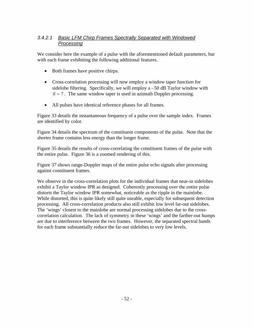
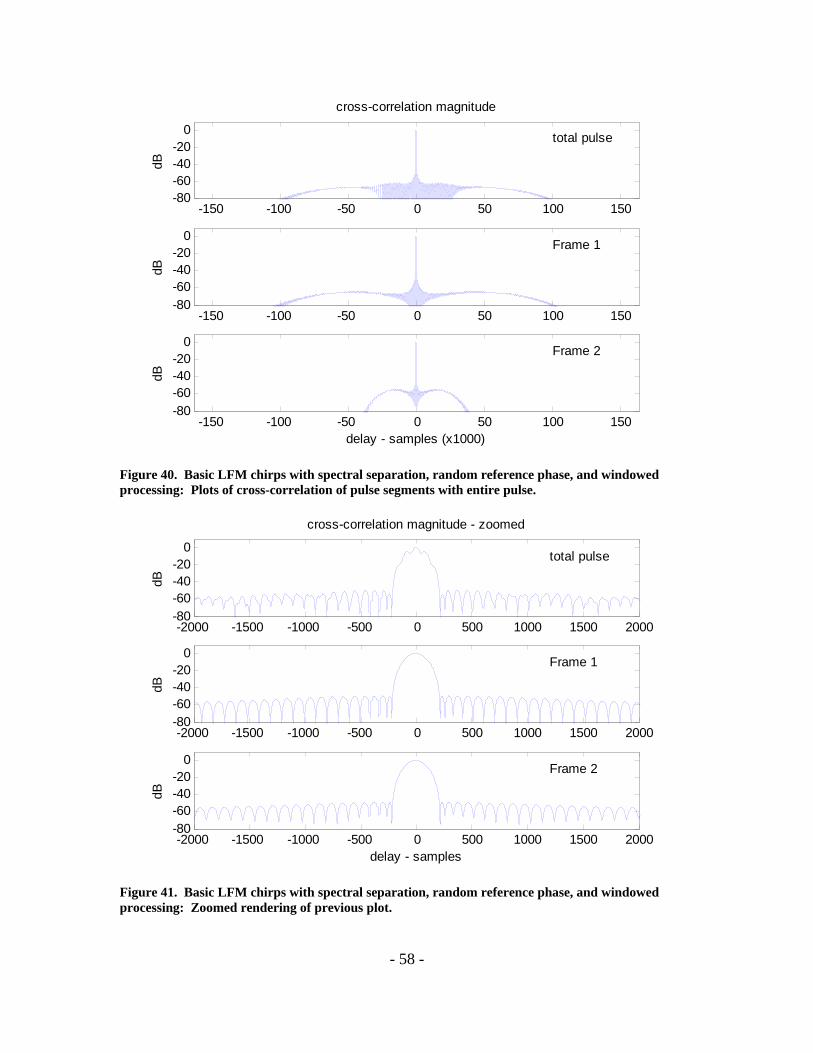
3.4.2.2 Basic LFM Chirp Frames Spectrally Separated with Random Reference Phase and Windowed Processing
We consider here the example of a pulse with the aforementioned default parameters, but with each frame exhibiting the following additional features.
Both frames have positive chirps.
Cross-correlation processing will now employ a window taper function for sidelobe filtering. Specifically, we will employ a 50 dB Taylor window with
7n . The same window taper is used in azimuth Doppler processing.
All pulses have independent random (uniformly distributed) reference phases for all frames.
Figure 38 details the instantaneous frequency of a pulse over the sample index. Frames are identified by color.
Figure 39 details the spectrum of the constituent components of the pulse. Note that the shorter frame contains less energy than the longer frame.
Figure 40 details the results of cross-correlating the constituent frames of the pulse with the entire pulse. Figure 41 is a zoomed rendering of this.
Figure 42 shows range-Doppler maps of the entire pulse echo signals after processing against constituent frames.
We observe in the cross-correlation plots for the individual frames that near-in sidelobes still exhibit a Taylor window IPR as designed. Coherently processing over the entire pulse still distorts the Taylor window IPR somewhat, noticeable as the ripple in the mainlobe. All cross-correlation products also still exhibit low level far-out sidelobes due to the cross-correlation calculation, but now these are fairly symmetric wings. The random reference phases for each pulse and frame reduces the interference between the two frames, rendering the IPR fairly symmetric for each cross-correlation. No interference between frames is discernible in these plots.
- 57 -
-80 -60 -40 -20 0 20 40 60 80485
490
495
500
505
510
515
sample index (x1000)
freq
uenc
y -
MH
z
instantaneous frequency
Frame 1
Frame 2
Figure 38. Basic LFM chirps with spectral separation, random reference phase, and windowed processing: Plot of instantaneous frequency vs. pulse sample index.
485 490 495 500 505 510 5150
10
20
30
40
50
60
70
80
90
100
mag
nitu
de -
dB
pulse/frame spectrum
frequency - MHz
total pulse
Frame 1Frame 2
Figure 39. Basic LFM chirps with spectral separation, random reference phase, and windowed processing: Plot of spectrums of pulse frames.
- 58 -
-150 -100 -50 0 50 100 150-80-60-40-20
0
dB
cross-correlation magnitude
total pulse
-150 -100 -50 0 50 100 150-80-60-40-20
0
dB
Frame 1
-150 -100 -50 0 50 100 150-80-60-40-20
0
dB
Frame 2
delay - samples (x1000)
Figure 40. Basic LFM chirps with spectral separation, random reference phase, and windowed processing: Plots of cross-correlation of pulse segments with entire pulse.
Figure 41. Basic LFM chirps with spectral separation, random reference phase, and windowed processing: Zoomed rendering of previous plot.
- 59 -
total pulse
-60 -30 0
Frame 1
-60 -30 0
Frame 2
-60 -30 0
Figure 42. Basic LFM chirps with spectral separation, random reference phase, and windowed processing: Result of Doppler processing of all pulses after respective cross-correlation operations against constituent frames. Colorbar values are dBc.
- 60 -
3.4.2.3 Shuffled Frequency Hops Spectrally Separated with Random Reference Phase and Windowed Processing
We consider here the example of a pulse with the aforementioned default parameters, but with each frame exhibiting the following additional features.
Each frame is composed of a shuffled stepped-chirp.
Cross-correlation processing will now employ a window taper function for sidelobe filtering. This is applied by weighting the individual chips of the reference function according to frequency. Specifically, we will employ a 50 dB Taylor window with 7n . The same window taper is used in azimuth Doppler processing.
All pulses have independent random reference phases for all frames.
Figure 43 details the instantaneous frequency of a single pulse over the sample index. Frames are identified by color.
Figure 44 details the mean energy spectrum of the constituent components of the pulse. Note that the shorter frame contains less energy than the longer frame.
Figure 45 details the results of cross-correlating the constituent frames of the pulse with the entire pulse. Figure 46 is a zoomed rendering of this.
Figure 47 shows range-Doppler maps of the entire pulse echo signals after processing against constituent frames.
We observe in the cross-correlation plots that the mainlobe and near-in sidelobes exhibit a Taylor window IPR down to a residual noise level that is typical of random signal waveforms. We note that the far-out sidelobes now exhibit a ‘shelf’ that is reduced from the case where both frames occupied the same spectral region. This shelf is still due to the frames interfering somewhat with each other because the relative bands exhibit edge slopes that overlap somewhat. A larger separation between bands would reduce the interference and hence the level of the shelf. The ripple in the mainlobe of the entire pulse would persist, but manifest at a higher frequency.
- 61 -
-80 -60 -40 -20 0 20 40 60 80485
490
495
500
505
510
515
sample index (x1000)
freq
uenc
y -
MH
z
instantaneous frequency
Frame 1
Frame 2
Figure 43. Shuffled frequency hops with spectral separation, random reference phase, and windowed processing: Plot of instantaneous frequency vs. pulse sample index for a single pulse.
485 490 495 500 505 510 5150
10
20
30
40
50
60
70
80
90
100
mag
nitu
de -
dB
pulse/frame spectrum
frequency - MHz
total pulse
Frame 1Frame 2
Figure 44. Shuffled frequency hops with spectral separation, random reference phase, and windowed processing: Plot of mean energy spectrums of pulse frames.
- 62 -
-150 -100 -50 0 50 100 150-80-60-40-20
0
dB
cross-correlation magnitude
total pulse
-150 -100 -50 0 50 100 150-80-60-40-20
0
dB
Frame 1
-150 -100 -50 0 50 100 150-80-60-40-20
0
dB
Frame 2
delay - samples (x1000)
Figure 45. Shuffled frequency hops with spectral separation, random reference phase, and windowed processing: Plots of cross-correlation of pulse segments with entire pulse.
Figure 46. Shuffled frequency hops with spectral separation, random reference phase, and windowed processing: Zoomed rendering of previous plot.
- 63 -
total pulse
-60 -30 0
Frame 1
-60 -30 0
Frame 2
-60 -30 0
Figure 47. Shuffled frequency hops with spectral separation, random reference phase, and windowed processing: Result of Doppler processing of all pulses after respective cross-correlation operations against constituent frames. Colorbar values are dBc.
- 64 -
3.5 Comments
We make a number of seemingly random observations here.
While we have exemplified the use of frames where each frame has the same resolution bandwidth, there is nothing inherent in the use of frames that compels us to do so. Essentially, if desired, different frames can have independently specified resolution bandwidths. More generally, individual frames may have entirely different frequency content from each other.
We have shown that individual frames may have different modulations employed. We further stipulate that different frames may use the same or different spectral shaping techniques, as may be desired for controlling processing sidelobes out of a matched filter. Individual frames might even exhibit different polarizations.
While we have discussed employing compound pulses for reasons of extending the range swath, especially to nearer ranges, we acknowledge that there may be other reasons for dividing a pulse into multiple frames. For example, reasons might include (but are not limited to) exploring or exploiting specific target phenomenology, clutter mitigation, signaling, and/or ambiguity mitigation.
The waveforms exemplified in this report displayed only two frames. However, these are easily extended to an arbitrary number of frames. For example, the sequential chirps of the earliest examples can be easily extended to manifest as an accelerating sawtooth pattern of instantaneous frequencies.
Some waveforms, notably noise and noise-like waveforms, lend themselves readily to processing against arbitrary frame sizes. That is, any frame size (usually larger than some minimum) of a noise waveform will have equal bandwidth, at least statistically, and therefor process to the same resolution.
We also acknowledge that there may be occasion when we might want to process subsets of the frames other than the ones exemplified.
- 65 -
4 Conclusions
We have proposed herein the following.
A pulse may be divided into multiple frames, where individual frames may exhibit different lengths, different modulations, and even non-overlapping spectral characteristics.
Latter frames can be processed to provide full-resolution range information at much nearer ranges than earlier frames, or the entire pulse.
Using and processing frames allows mitigating the typical constraint of near-range operation with long-pulses. This allows extending the range swath for which a pulse may be processed to full resolution.
Additional benefit can be derived from appropriate random reference phases that change with frame as well as pulse number.
- 66 -
“Success is the sum of details.” -- Harvey S. Firestone
- 67 -
Appendix A – Details of 50 dB Taylor Window (nbar = 7)
0 1 2 3 4 5 6 7 8 9 10-80
-60
-40
-20
0taylor, -50 dB, nbar=7
dB
10-1
100
101
102
103
-80
-60
-40
-20
0
dB
axis units normalized to -3 dB width
window IPR -3 dB bin bandwidth = 1.3599 (corresponds to sinc width of 0.8845)window IPR -18 dB rel bandwidth = 2.2755 (normalized to -3 dB width)window IPR first null = 1.5942 (normalized)window SNR gain = -1.5421 dBwindow PSL = -50.0746 dBcwindow ISL = -39.9325 dBc from 1.5942 outward
Figure 48. This window taper function is used in the examples throughout this report.
- 68 -
“We're all working together; that's the secret.” -- Sam Walton
- 69 -
References
1 Andrija P. Petrovic, Aleksa J. Zejak, Bojan Zrnic, “ECF filter design for radar applications”, Proceedings of the 6th IEEE International Conference on Electronics, Circuits and Systems (ICECS '99), Vol. 2, pp. 663-666, 5-8 September 1999.
2 S.P. Kalenichenko, V.N. Mikhailov, “The Joint Radar Targets Detecting and Communication System”, Proceedings of the International Radar Symposium (IRS 2006), pp. 1-4, 24-26 May 2006.
3 R. Benjamin, “Recent developments in radar modulation and processing techniques”, Electronics and Power, Vol. 10, Issue 12, pp. 435-438, December 1964.
4 Christopher D. Ziomek, Emily S. Jones, “Advanced waveform generation techniques for ATE”, Proceedings of the 2009 IEEE AUTOTESTCON, pp. 269-274, 14-17 Sept. 2009.
5 Ying Li, William Moran, Sandeep P. Sira, Antonia Papandreou-Suppappola, Darryl Morrell, “Adaptive Waveform Design in Rapidly-Varying Radar Scenes”, Proceedings of the 2009 International Waveform Diversity and Design (WD&D) Conference, pp. 263-267, 8-13 Feb. 2009.
6 Bill Dawber, Ian Nichols, “Digital pulse compressor design for ultra-low range sidelobes for use within the eclipsed region”, Proceedings of the 2007 IET International Conference on Radar Systems, pp. 1-5, 15-18 Oct. 2007.
7 Stephen Harman, “The Performance of a Novel Three-Pulse Radar Waveform for Marine Radar Systems”, Proceedings of the 5th European Radar Conference (EuRAD 2008), pp. 160-163, Amsterdam, The Netherlands, October 2008.
8 Gerhard Krieger, Nicolas Gebert, Alberto Moreira, “Multidimensional Waveform Encoding: A New Digital Beamforming Technique for Synthetic Aperture Radar Remote Sensing”, IEEE Transactions On Geoscience And Remote Sensing, Vol. 46, No. 1, pp. 31-46, January 2008.
9 Armin W. Doerry, Brandeis Marquette, “Shaping the Spectrum of Random-Phase Radar Waveforms”, Sandia Report SAND2012-6915, Unlimited Release, August 2012.
10 Armin W. Doerry, “Generating Nonlinear FM Chirp Waveforms for Radar”, Sandia Report SAND2006-5856, Unlimited Release, September 2006.
11 Armin W. Doerry, “SAR Processing with Non-Linear FM Chirp Waveforms”, Sandia Report SAND2006-7729, Unlimited Release, December 2006.
- 70 -
Distribution
Unlimited Release
1 MS 0532 J. J. Hudgens 5240
1 MS 0519 J. A. Ruffner 5349 1 MS 0519 A. W. Doerry 5349 1 MS 0519 L. Klein 5349
1 MS 0899 Technical Library 9536 (electronic copy)
1 Brandeis Marquette (electronic copy) General Atomics ASI, RSG 16868 Via Del Campo Ct San Diego, CA 92127
1 John Fanelle (electronic copy) General Atomics ASI, RSG 16761 Via Del Campo Ct San Diego, CA 92127