Compressible Duct Flow with Friction

We treat only the effect of friction, neglecting area change and heat transfer.

The basic assumptions are 1. Steady one-dimensional adiabatic flow 2. Perfect gas with constant specific heats 3. Constant-area straight duct 4. Negligible shaft-work and potential-energy changes 5. Wall shear stress correlated by a Darcy friction factor

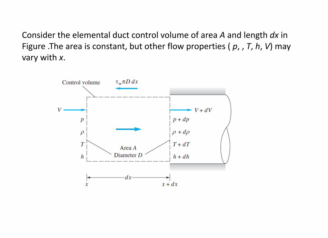
Consider the elemental duct control volume of area A and length dx in Figure .The area is constant, but other flow properties ( p, , T, h, V) may vary with x.

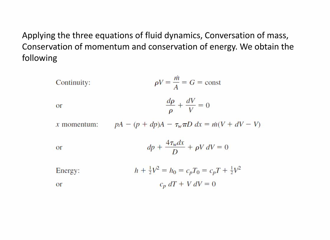
Applying the three equations of fluid dynamics, Conversation of mass, Conservation of momentum and conservation of energy. We obtain the following

Applying the three equations of fluid dynamics, Conversation of mass, Conservation of momentum and conservation of energy. We obtain the following

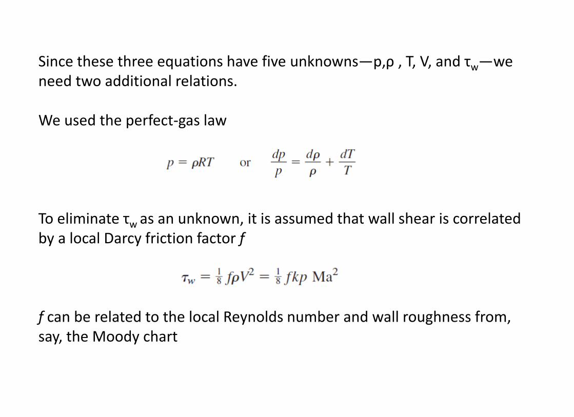
Since these three equations have five unknowns—p,ρ , T, V, and τw—we need two additional relations. We used the perfect-gas law To eliminate τw as an unknown, it is assumed that wall shear is correlated by a local Darcy friction factor f f can be related to the local Reynolds number and wall roughness from, say, the Moody chart

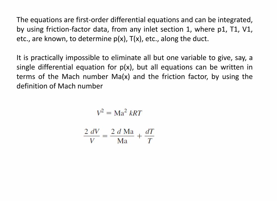
The equations are first-order differential equations and can be integrated, by using friction-factor data, from any inlet section 1, where p1, T1, V1, etc., are known, to determine p(x), T(x), etc., along the duct. It is practically impossible to eliminate all but one variable to give, say, a single differential equation for p(x), but all equations can be written in terms of the Mach number Ma(x) and the friction factor, by using the definition of Mach number

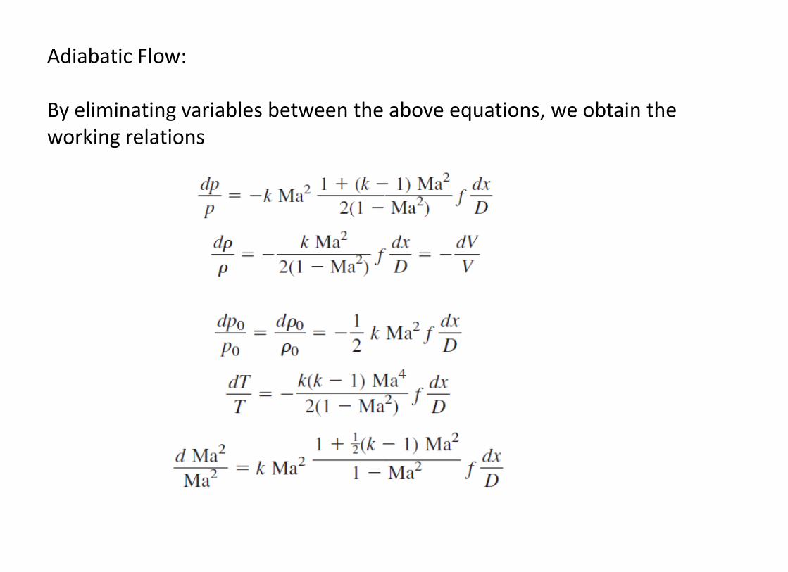
Adiabatic Flow: By eliminating variables between the above equations, we obtain the working relations

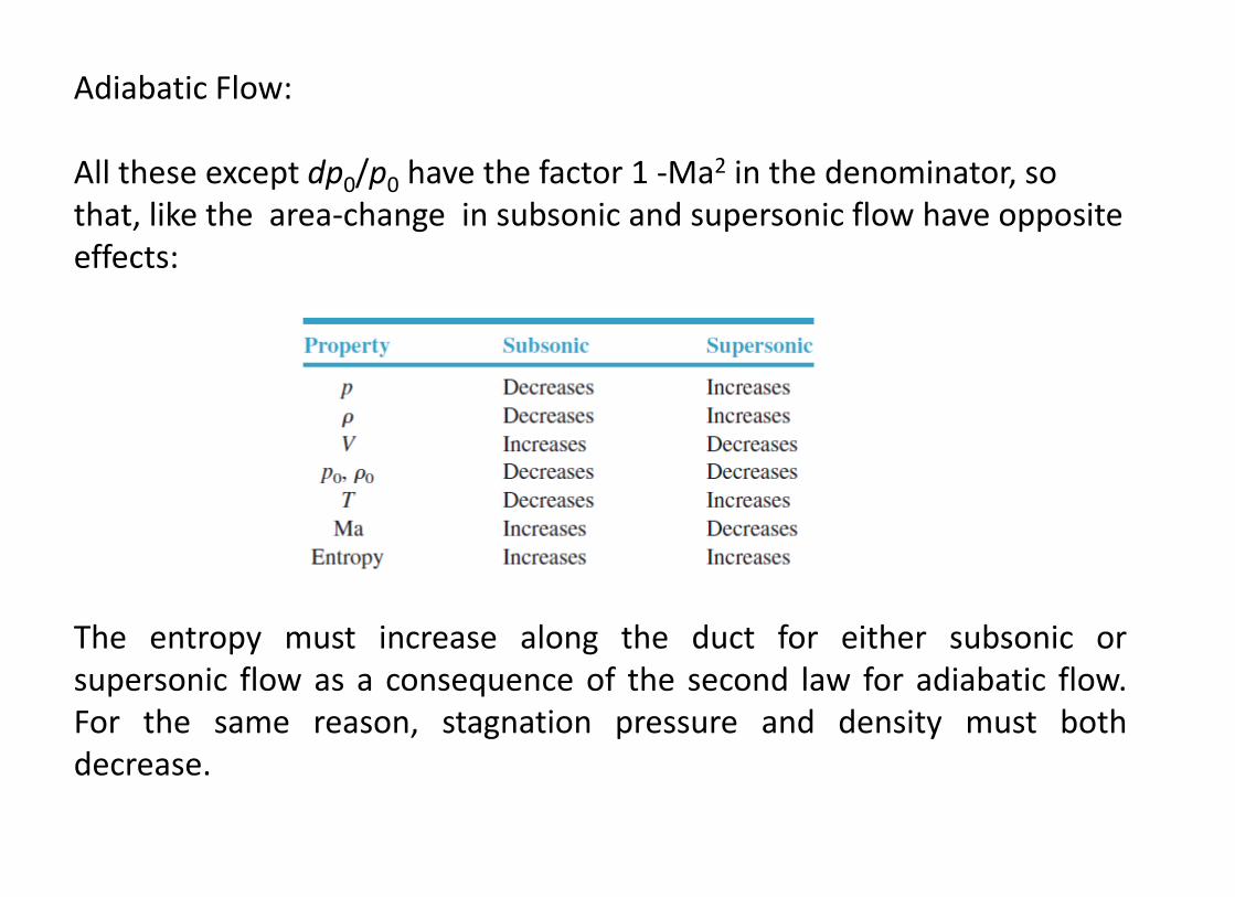
Adiabatic Flow: All these except dp0/p0 have the factor 1 -Ma2 in the denominator, so that, like the area-change in subsonic and supersonic flow have opposite effects: The entropy must increase along the duct for either subsonic or supersonic flow as a consequence of the second law for adiabatic flow. For the same reason, stagnation pressure and density must both decrease.

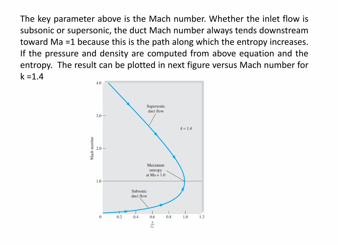
The key parameter above is the Mach number. Whether the inlet flow is subsonic or supersonic, the duct Mach number always tends downstream toward Ma =1 because this is the path along which the entropy increases. If the pressure and density are computed from above equation and the entropy. The result can be plotted in next figure versus Mach number for k =1.4

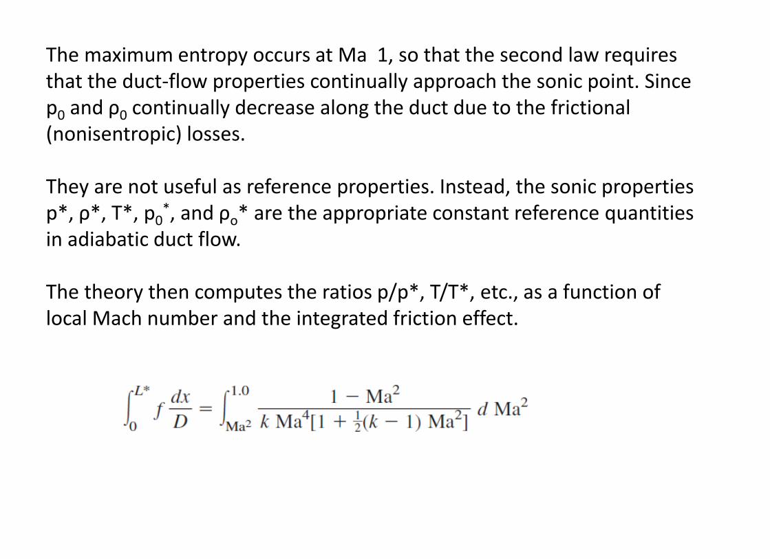
The maximum entropy occurs at Ma 1, so that the second law requires that the duct-flow properties continually approach the sonic point. Since p0 and ρ0 continually decrease along the duct due to the frictional (nonisentropic) losses. They are not useful as reference properties. Instead, the sonic properties p*, ρ*, T*, p0

*, and ρo* are the appropriate constant reference quantities in adiabatic duct flow. The theory then computes the ratios p/p*, T/T*, etc., as a function of local Mach number and the integrated friction effect.

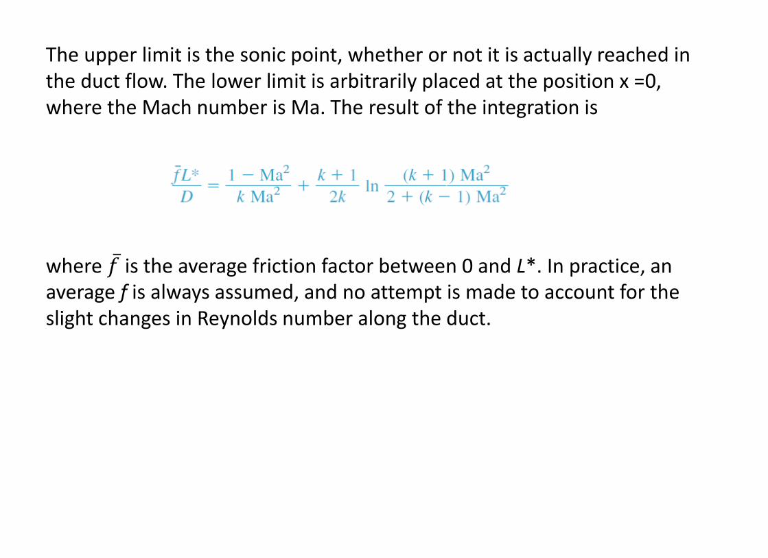
The upper limit is the sonic point, whether or not it is actually reached in the duct flow. The lower limit is arbitrarily placed at the position x =0, where the Mach number is Ma. The result of the integration is where 𝑓 is the average friction factor between 0 and L*. In practice, an average f is always assumed, and no attempt is made to account for the slight changes in Reynolds number along the duct.

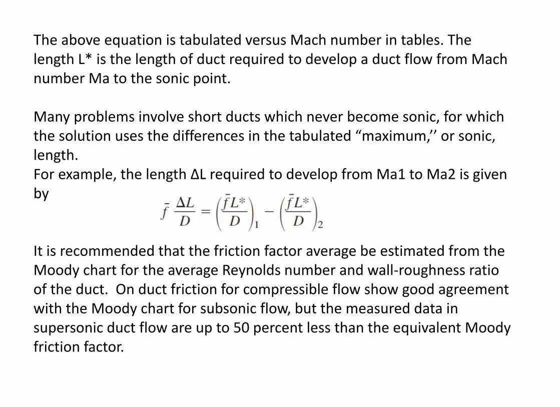
The above equation is tabulated versus Mach number in tables. The length L* is the length of duct required to develop a duct flow from Mach number Ma to the sonic point. Many problems involve short ducts which never become sonic, for which the solution uses the differences in the tabulated “maximum,’’ or sonic, length. For example, the length ΔL required to develop from Ma1 to Ma2 is given by It is recommended that the friction factor average be estimated from the Moody chart for the average Reynolds number and wall-roughness ratio of the duct. On duct friction for compressible flow show good agreement with the Moody chart for subsonic flow, but the measured data in supersonic duct flow are up to 50 percent less than the equivalent Moody friction factor.