Comput. Methods Appl. Mech. Engrg. - University of Cincinnatiliugr/Publications/Journal...

Comput. Methods Appl. Mech. Engrg. 198 (2009) 3479–3498

Contents lists available at ScienceDirect

Comput. Methods Appl. Mech. Engrg.

journal homepage: www.elsevier .com/locate /cma

A face-based smoothed finite element method (FS-FEM) for visco-elastoplasticanalyses of 3D solids using tetrahedral mesh

T. Nguyen-Thoi a,c,*, G.R. Liu a,b, H.C. Vu-Do a,c, H. Nguyen-Xuan b,c

a Center for Advanced Computations in Engineering Science (ACES), Department of Mechanical Engineering, National University of Singapore,9 Engineering Drive 1, Singapore 117576, Singaporeb Singapore-MIT Alliance (SMA), E4-04-10, 4 Engineering Drive 3, Singapore 117576, Singaporec Faculty of Mathematics and Computer Science, University of Science, Vietnam National University-HCM, Viet Nam

a r t i c l e i n f o

Article history:Received 27 April 2009Received in revised form 27 June 2009Accepted 8 July 2009Available online 12 July 2009

Keywords:Numerical methodsMeshfree methodsFace-based smoothed finite elementmethod (FS-FEM)Finite element method (FEM)Strain smoothing techniqueVisco-elastoplastic analyses

0045-7825/$ - see front matter � 2009 Elsevier B.V. Adoi:10.1016/j.cma.2009.07.001

* Corresponding author. Address: Department of Mmatics and Computer Science, University of Science, VHCM, Vietnam, 227 Nguyen Van Cu street, District 5Tel.: + 84 (0)942340411.

E-mail addresses: [email protected](T. Nguyen-Thoi).

a b s t r a c t

A face-based smoothed finite element method (FS-FEM) using tetrahedral elements was recently pro-posed to improve the accuracy and convergence rate of the existing standard finite element method(FEM) for the solid mechanics problems. In this paper, the FS-FEM is further extended to more compli-cated visco-elastoplastic analyses of 3D solids using the von-Mises yield function and the Prandtl–Reussflow rule. The material behavior includes perfect visco-elastoplasticity and visco-elastoplasticity withisotropic hardening and linear kinematic hardening. The formulation shows that the bandwidth of stiff-ness matrix of FS-FEM is larger than that of FEM, and hence the computational cost of FS-FEM in numer-ical examples is larger than that of FEM for the same mesh. However, when the efficiency of computation(computation time for the same accuracy) in terms of a posteriori error estimation is considered, the FS-FEM is more efficient than the FEM.

� 2009 Elsevier B.V. All rights reserved.

1. Introduction

Recently years, significant development has been made inmeshfree methods in term of theory, formulism and application[1]. Some of these meshfree techniques have been applied backto finite element settings [2]. The strain smoothing technique hasbeen proposed by Chen et al. [3] to stabilize the solutions of the no-dal integrated meshfree methods and then applied in the natural-element method [4]. Liu et al. has generalized the gradient (strain)smoothing technique [5] and applied it in the meshfree context[6–13] to formulate the node-based smoothed point interpolationmethod (NS-PIM or LC-PIM) [14,15] and the node-based smoothedradial point interpolation method (NS-RPIM or LC-RPIM) [16].Applying the same idea to the FEM, a cell-based smoothed finiteelement method (SFEM or CS-FEM) [17–20], a node-basedsmoothed finite element method (NS-FEM) [21] and an edge-basedsmoothed finite element method (ES-FEM) in two-dimensional(2D) problems [22] have also been formulated.

ll rights reserved.

echanics, Faculty of Mathe-ietnam National University-, Hochiminh city, Viet Nam.

, [email protected]

In the CS-FEM, the domain discretization is still based on quad-rilateral elements as in the FEM, however the stiffness matrices arecalculated based over smoothing cells (SC) located inside the quad-rilateral elements as shown in Fig. 1. When the number of SC of theelements equals 1, the CS-FEM solution has the same propertieswith those of FEM using reduced integration. The CS-FEM in thiscase can be unstable and can have spurious zeros energy modes,depending on the setting of the problem. A stabilization techniqueto alleviate this instability can be found in ref [27] which can be ex-tended for 3D finite elements and for plasticity problems. When SCapproaches infinity, the CS-FEM solution approaches to the solu-tion of the standard displacement compatible FEM model [18]. Inpractical calculation, using four smoothing cells for each quadrilat-eral element in the CS-FEM is easy to implement, work well in gen-eral and hence advised for all problems. The numerical solution ofCS-FEM (SC = 4) is always stable, accurate, much better than that ofFEM, and often very close to the exact solutions. The CS-FEM hasbeen extended for general n-sided polygonal elements (nSFEM ornCS-FEM) [28], dynamic analyses [29], incompressible materialsusing selective integration [30,31], plate and shell analyses[32–36], and further extended for the extended finite elementmethod (XFEM) to solve fracture mechanics problems in 2Dcontinuum and plates [37].

In the NS-FEM, the domain discretization is also based on ele-ments as in the FEM, however the stiffness matrices are calculated

http://dx.doi.org/10.1016/j.cma.2009.07.001

mailto:[email protected]

mailto:[email protected]

http://www.sciencedirect.com/science/journal/00457825

http://www.elsevier.com/locate/cma

1 5

8

d

9

47

2

3

6

1 5

b 46

2

3

1

e 4

2

3

1 5

c

8

47

2

3

6

y

x

3

1 2

f 4

: added nodes to form the smoothing cells

3

: field nodes

x

y

1 2

a 4

Fig. 1. Division of quadrilateral element into the smoothing cells (SCs) in CS-FEM by connecting the mid-segment-points of opposite segments of smoothing cells. (a) 1 SC; (b)2 SCs; (c) 3 SCs; (d) 4 SCs; (e) 8 SCs; and (f) 16 SCs.

3480 T. Nguyen-Thoi et al. / Comput. Methods Appl. Mech. Engrg. 198 (2009) 3479–3498

based on smoothing domains associated with nodes. The NS-FEMworks well for triangular elements, and can be applied easily togeneral n-sided polygonal elements [21] for 2D problems and tet-rahedral elements for 3D problems. For n-sided polygonal ele-ments [21], smoothing domain XðkÞ associated with the node k iscreated by connecting sequentially the mid-edge-point to the cen-tral points of the surrounding n-sided polygonal elements of thenode k as shown in Fig. 2. Note that n-sided polygonal elementswere also formulated in standard FEM settings [38–41]. When onlylinear triangular or tetrahedral elements are used, the NS-FEM pro-duces the same results as the method proposed by Dohrmann et al.[42] or to the NS-PIM (or LC-PIM) [14] using linear interpolation.The NS-FEM [21] has been found immune naturally from volumet-ric locking and possesses the upper bound property in strain en-ergy as presented in [43]. Hence, by combining the NS-FEM andFEM with a scale factor a 2 ½0;1�, a new method named as the al-

node k

cell(k)

(k)Γ

: central point of n-sided polygonal element : field node : mid-edge point

Fig. 2. n-Sided polygonal elements and the smoothing cell (shaded area) associatedwith nodes in NS-FEM.

pha Finite Element Method (aFEM) [44] is proposed to obtainnearly exact solutions in strain energy using triangular and tetra-hedral elements. The aFEM [44] is therefore also a good candidateamong the methods having super convergence and high efficiencyin non-linear problems [45–47]. The NS-FEM has been developedfor adaptive analysis [48]. One disadvantage of NS-FEM is its largerbandwidth of stiffness matrix compared to that of FEM, becausethe number of nodes related to the smoothing domains associatedwith nodes is larger than that related to the elements. The compu-tational cost of NS-FEM therefore is larger than that of FEM for thesame meshes used. In terms of computational efficiency (CPU timeneeded for the same accuracy results measured in energy norm),however, the NS-FEM-T3 can be much better than the FEM-T3(see, Chapter 8 in [1]).

In the ES-FEM [22], the problem domain is also discretizedusing triangular elements as in the FEM, however the stiffnessmatrices are calculated based on smoothing domains associatedwith the edges of the triangles. For triangular elements, thesmoothing domain XðkÞ associated with the edge k is created byconnecting two endpoints of the edge to the centroids of the adja-cent elements as shown in Fig. 3. The numerical results of ES-FEMusing examples of static, free and forced vibration analyses of sol-ids [22] demonstrated the following excellent properties: (1) theES-FEM is often found super-convergent and much more accuratethan the FEM using triangular elements (FEM-T3) and even moreaccurate than the FEM using quadrilateral elements (FEM-Q4) withthe same sets of nodes; (2) there are no spurious non-zeros energymodes and hence the ES-FEM is both spatial and temporal stableand works well for vibration analysis; (3) no additional degree offreedom and no penalty parameter is used; (4) a novel domain-based selective scheme is proposed leading to a combined ES/NS-FEM model that is immune from volumetric locking and henceworks very well for nearly incompressible materials. Note thatsimilar to the NS-FEM, the bandwidth of stiffness matrix in theES-FEM is larger than that in the FEM-T3, hence the computationalcost of ES-FEM is larger than that of FEM-T3. However, when theefficiency of computation (computation time for the same accu-racy) in terms of both energy and displacement error norms is con-sidered, the ES-FEM is more efficient [22]. The ES-FEM has beendeveloped for 2D piezoelectric [23], 2D visco-elastoplastic [24],plate [25] and primal-dual shakedown analyses [26].

C E

G

: centroid of triangles (I , O, H ): field node

boundary edge m (AB)

inner edge k (DF)

(k)

(k)Γ

Γ(m)

(m)

A

B

D

F

H

O

I

(lines: DH , HF , FO, OD)

(4-node domain DHFO)

(lines: AB, BI , IA)

(triangle ABI )

Fig. 3. Triangular elements and the smoothing domains (shaded areas) associated with edges in ES-FEM.

T. Nguyen-Thoi et al. / Comput. Methods Appl. Mech. Engrg. 198 (2009) 3479–3498 3481

Further more, the idea of ES-FEM has been extended for the 3Dproblems using tetrahedral elements to give a so-called the face-based smoothed finite element method (FS-FEM) [49]. In theFS-FEM, the domain discretization is still based on tetrahedralelements as in the FEM, however the stiffness matrices are calcu-lated based on smoothing domains associated with the faces ofthe tetrahedral elements as shown in Fig. 4. The FS-FEM is foundsignificantly more accurate than the FEM using tetrahedral ele-ments for both linear and geometrically non-linear solid mechanicsproblems. In addition, a novel domain-based selective scheme isproposed leading to a combined FS/NS-FEM model that is immunefrom volumetric locking and hence works well for nearly incom-pressible materials. The implementation of the FS-FEM is straight-forward and no penalty parameters or additional degrees offreedom are used. Note that similar to the ES-FEM and NS-FEM,the bandwidth of stiffness matrix in the FS-FEM is also larger thanthat in the FEM, and hence the computational cost of FS-FEM is lar-ger than that of FEM. However, when the efficiency of computation(computation time for the same accuracy) in terms of both energyand displacement error norms is considered, the FS-FEM is stillmore efficient than the FEM [49].

In this paper, we aim to extend the FS-FEM to even more com-plicated visco-elastoplastic analyses in 3D solids. In this work, wecombine the FS-FEM with the work of Carstensen and Klose [50]using the standard FEM in the setting of von-Mises conditions

: central point of elements (H, I): field node

interface k

associated with interface k

smoothed domain (k)

element 1

element 2

A

B

C

D

E

(triangle BCD)

(tetrahedron ABCD)

(tetrahedron BCDE)

HI

(BCDIH)

of two combined tetrahedrons

Fig. 4. Two adjacent tetrahedral elements and the smoothing domain XðkÞ (shadeddomain) formed based on their interface k in the FS-FEM

and a Prandtl–Reuss flow rule. The material behavior includes per-fect visco-elastoplasticity and visco-elastoplasticity with isotropichardening and linear kinematic hardening in a dual model withboth displacements and the stresses as the main variables. Thenumerical procedure, however, eliminates the stress variablesand the problem becomes only displacement-dependent and iseasier to deal with. The formulation shows that the bandwidth ofstiffness matrix of FS-FEM is larger than that of FEM, and hencethe computational cost of FS-FEM in numerical examples is largerthan that of FEM. However, when the efficiency of computation(computation time for the same accuracy) in terms of a posteriorierror estimation is considered, the FS-FEM is more efficient thanthe FEM.

2. Dual model of visco-elastoplastic problem using the FS-FEM

2.1. Strong form and weak form [50]

The visco-elastoplastic problem which deforms in the intervalt 2 ½0; T� can be described by equilibrium equation in the domainX bounded by C

divrþ b ¼ 0 in X ð1Þ

where b 2 ðL2ðXÞÞ3 is the body forces, r 2 ðL2ðXÞÞ3 is the stress field.The essential and static boundary conditions, respectively, on theDirichlet boundary CD and the Neumann boundary CN are

u ¼ w0 on CD and rn ¼ �t on CN ð2Þ

in which u 2 ðH1ðXÞÞ3 is the displacement field; w0 2 ðH1ðXÞÞ3 isprescribed surface displacement; �t 2 ðL2ðCNÞÞ3 is prescribed surfaceforce and n is the unit outward normal matrix.

In the context of small strain, the total strain eðuÞ ¼ rSu, whererSu denotes the symmetric part of displacement gradient, is sep-arated into two contributions

eðuÞ ¼ eðrÞ þ pðnÞ ð3Þ

where eðrÞ ¼ C�1r is elastic strain tensor; n is internal variable and

pðnÞ is an irreversible plastic strain in which C is a fourth order ten-sor of material constants.

To describe properly the evolution process for the plastic strain,it is required to define the admissible stresses, a yield function, andan associated flow rule. In this work, we use the von-Mises yieldfunction and the Prandtl–Reuss flow rule. Let p and n be the kine-matic variables of the generalized strain P ¼ ðp; nÞ, and R ¼ ðr; aÞ


be the corresponding generalized stress, where a is the hardeningparameter describing internal stresses. We define � to be theadmissible stresses set, which is a closed, convex set, containing0, and defined by

� ¼ fR : UðRÞ 6 0g ð4Þ

where U is the von-Mises yield function which is presented specif-ically for different visco-elastoplasticity cases as follows:

Case a: Perfect visco-elastoplasticity:In this case, there is no hardening and the internal variables n, a

are absent. The von-Mises yield function is given simply by

UðrÞ ¼ kdevðrÞk � rY ð5Þ

where rY is the yield stress; kxk is the norm of tensor x and is com-

puted by kxk ¼ffiffiffiffiffiffiffiffiffiffiffiffiffiffiffiffiffiffiffiffiffiffiffiffiffiffiP3

i¼1

P3j¼1x2

ij

q, devðxÞ is the deviator tensor of ten-

sor x and defined by

devðxÞ ¼ x� trðxÞ3

I ð6Þ

in which I is the second-order symmetric unit tensor andtrðxÞ ¼

P3i¼1xii is the trace operator of tensor x. For the viscosity

parameter v > 0, the Prandtl–Reuss flow rule has the form

_p ¼1v ðkdevðrÞk � rYÞ if kdevðrÞk > rY

0 if kdevðrÞk 6 rY

(ð7Þ

Case b: Visco-elastoplasticity with isotropic hardening:In the case of the isotropic hardening, the problem is character-

ized by a modulus of hardening H P 0, and a � aI P 0 (I meansIsotropic) becomes a scalar hardening parameter and relates tothe scalar internal strain variable n by

aI ¼ �H1n ð8Þ

where H1 is a positive hardening parameter.The von-Mises yield function is given by

Uðr;aIÞ ¼ kdevðrÞk � rYð1þ HaIÞ ð9Þ

For the viscosity parameter v > 0, the Prandtl–Reuss flow rule hasthe form

_p_n

� �¼

1v

11þH2r2

Yð ÞkdevðrÞk�ð1þaIHÞrY

�HrY ðkdevðrÞk�ð1þaIHÞrY Þ

� �if kdevðrÞk> ð1þaIHÞrY

00

� �if kdevðrÞk6 ð1þaIHÞrY

8>>><>>>: ð10Þ

Case c: Visco-elastoplasticity with linear kinematic hardening:In the case of the linear kinematic hardening, the internal stress

a � aK (K means Kinematic) relates to the internal strain n by

aK ¼ �k1n ð11Þ

where k1 is a positive parameter.The von-Mises yield function is given by

Uðr; aKÞ ¼ kdevðrÞ � devðaKÞk � rY ð12Þ

For the viscosity parameter v > 0, the Prandtl–Reuss flow rule hasthe form

_p_n

� �¼

12vkdevðr� aKÞk � rY

�ðkdevðr� aKÞk � rYÞ

� �if kdevðr� aKÞk > rY

00

� �if kdevðr� aKÞk 6 rY

8>>><>>>:ð13Þ

In general, the Prandtl–Reuss flow rule, with the viscosity parame-ter v > 0, has the form [50]

_p_n

� �¼ 1

vr�Pr

a�Pa

� �ð14Þ

where Pr and Pa are defined as the projections of ðr; aÞ into theadmissible stresses set � .

The visco-elastoplastic problem can now be stated generally ina weak formulation with the above-mentioned flow rules as fol-lows: seek u 2 ðH1ðXÞÞ3 such that u = w0 on CD and for8v 2 ðH1

0ðXÞÞ3 ¼ fv 2 ðH1ðXÞÞ3 : v ¼ 0 on CDg, the following equa-

tions are satisfied:ZX

rðuÞ : eðvÞdX ¼Z

Xb � v dXþ

ZCN

�t � v dC ð15Þ

_p_n

� �¼ eð _uÞ � C�1 _r

nð _aÞ

" #¼ 1

vr�Pr

a�Pa

� �ð16Þ

where A : B ¼P

j;kAjkBjk denotes the scalar products of (symmetric)matrices.

2.2. Time-discretization scheme [50]

A generalized midpoint rule is used as the time-discretizationscheme. In each time step, a spatial problem needs to be solvedwith given variables ðuðtÞ; rðtÞ; aðtÞÞ at time t0 denoted asðu0; r0; a0Þ and unknowns at time t1 ¼ t0 þ Dt denoted asðu1; r1; a1Þ. Time derivatives are replaced by backward differencequotients; for instance _u is replaced by u#�u0

#Dt whereu# ¼ ð1� #Þu0 þ #u1 with 1=2 6 # 6 1. The time discrete problemnow becomes: seek u# 2 ðH1ðXÞÞ3 that satisfied u# ¼ w0 on CD andZ

Xrðu#Þ : eðvÞdX ¼

ZX

b# � vdXþZ

CN

�t# � vdC;8v 2 H10ðXÞ

� �3 ð17Þ

1#Dt

eðu# � u0Þ � C�1ðr# � r0Þnða; t#Þ � nða; t0Þ

" #¼ 1

vr# �Pr#

a# �Pa#

� �ð18Þ

where b# ¼ ð1� #Þb0 þ #b1;�t# ¼ ð1� #Þ�t0 þ #�t1 in which b0;�t0;b1

and �t1 are body forces and surface forces at time t0; t1, respectively.Eqs. (17) and (18) is in fact a dual model that has both stress and

displacement as field variables. To solve the set of Eqs. (17) and(18) efficiently, we need to eliminate one variable. This can be doneby first expressing explicitly the stress r# in the form of displace-ment u# using Eq. (18), and then substituting it into Eq. (17). Theproblem will then becomes only displacement-dependent, andwe need to solve the resultant form of Eq. (17).

2.3. Analytic expression of the stress tensor

Explicit expressions for the stress tensor r# in different cases ofvisco-elastoplasticity can be presented briefly as follows [50]

(a) Perfect visco-elastoplasticity:In the elastic phase

r# ¼ C1 trð#DtAÞIþ 2l devð#DtAÞ ð19Þwhere A ¼ eðu#�u0Þ

#Dt þ C�1 r0#Dt :

In the plastic phase, the plastic occurs when kdevð#DtAÞk > brY and

r# ¼ C1trð#DtAÞIþ ðC2 þ C3=kdevð#DtAÞkÞdevð#DtAÞ ð20ÞwhereC1 ¼ kþ 2l=3; C2 ¼ v=ðbv þ #DtÞ; C3 ¼ #DtrY=ðbv þ #DtÞ

ð21Þin which b ¼ 1=ð2lÞ.

(b) Visco-elastoplasticity with isotropic hardening:In the elastic phase

r# ¼ C1 trð#DtAÞIþ 2l devð#DtAÞ ð22Þ

In the plastic phase, the plastic occurs when kdevð#DtAÞk >bð1þ aI

0HÞrY and


r# ¼ C1 trð#DtAÞIþ ðC3=ðC2kdevð#DtAÞkÞ þ C4=C2Þdevð#DtAÞ ð23Þwhere

C1 ¼ kþ 2l=3;C2 ¼ bvð1þ H2r2Y Þ þ #Dtð1þ bH1H2r2

YÞC3 ¼ #DtrY ð1þ aI

0HÞ;C4 ¼ H1H2#Dtr2Y þ vð1þ H2r2

Y Þ ð24Þ

in which aI0 is the initial scalar hardening parameter.

(c) Visco-elastoplasticity with linear kinematic hardening:In the elastic phase

r# ¼ C1 trð#DtAÞIþ 2l devð#DtAÞ ð25ÞIn the plastic phase, the plastic occurs when kdevð#DtA�baK

0 Þk > brY and

r# ¼ C1 tr #DtAð ÞIþ C2 þ C3=kdev #DtA� baK0

� �k

� �dev #DtA� baK

0

� �þ dev aK

0

� �ð26Þ

Fig. 5. Flow chart to solve the visco-elastopla

where

C1 ¼ kþ 2l=3; C2 ¼#Dtk1 þ 2v

#Dt þ b#Dtk1 þ v=l ;

C3 ¼#DtrY

#Dt þ b#Dtk1 þ v=l ð27Þ

in which rk0 is the initial internal stress.

Now, by replacing the stress r# described explicitly into Eq. (17),we obtain the only displacement-dependent problem and can ap-ply different numerical methods to solve.

2.4. Discretization in space using FEM

The domain X is now discretized into Ne elements and Nn nodessuch that X ¼

SNee¼1Xe and Xi \Xj ¼ ;; i – j. In the discrete version

of (17), the spaces V ¼ ðH1ðXÞÞ3 and V0 ¼ ðH10ðXÞÞ

3 are replaced

stic problems using the FS-FEM: part 1.


by finite dimensional subspaces Vh � V and Vh0 � V0. The discrete

problem now becomes: seek u# 2 Vh such that u# ¼ w0 on CD andZX

r#ðeðu# � u0Þ þ C�1r0Þ : eðvÞdX

¼Z

Xb# � v dXþ

ZCN

�t# � v dC for 8v 2 Vh0 ð28Þ

Let ðu1; . . . ;u3NnÞ be the nodal basis of the finite dimensional space

Vh, where ui is the independent scalar hat shape function on nodesatisfying condition Kronecker uiðiÞ ¼ 1 and uiðjÞ ¼ 0; i–j, then thediscrete problem Eq. (28) now becomes: seeking u# 2 Vh such thatu# ¼ w0 on CD and

Fi ¼Z

Xr#ðeðu# � u0Þ þ C�1

r0Þ

: eðuiÞdX�Z

Xb# �ui dX�

ZCN

�t# �ui dC ¼ 0 ð29Þ

Fig. 6. Flow chart to solve the visco-elastopla

for i ¼ 1; . . . ;3Nn. Fi in Eq. (29) can be written in the sum of a part Q i

which depends on u# and a part Pi which is independent of u# suchas

Fiðu#Þ ¼ Q iðu#Þ � Pi ð30Þ

with

Q iðu#Þ ¼ Q i ¼Z

Xr# eðu# � u0Þ þ C�1

r0

: eðuiÞdX ð31Þ

Pi ¼Z

Xb# �uidXþ

ZCN

�t# �ui dC ð32Þ

2.5. Iterative solution

In order to solve Eq. (29) in this work, Newton–Raphson methodis used [50]. In each step of the Newton iterations, the discrete

stic problems using the FS-FEM: part 2.

y

g(t)(2,2,0.5)

Β

x(0,0,0.5)a Α

x

2

g(t)y 2

cbaFig. 7. Thick plate with a cylindrical hole subjected to time dependent surface forces gðtÞ 3D full model without forces; (b) model with forces viewed from the positivedirection of z-axis; and (c) one eighth of model with forces and symmetric boundary conditions viewed from the positive direction of z-axis.


displacement vector up# expressed in the nodal basis by

up# ¼

P3Nni¼1 uiui is determined from iterative solution

DFðup#Þu

pþ1# ¼ DFðup

#Þup# � Fðup

#Þ ð33Þ

where DF is in fact the system stiffness matrix whose the local en-tries are defined as

DF up#;1; . . . ; up

#;3Nn

rs¼ @Fr up

#;1; . . . ; up#;3Nn

=@up

#;s ð34Þ

where r; s 2 Wdf which is the set containing degrees of freedom ofall of nodes.

To properly apply the Dirichlet boundary conditions for ournonlinear problem, we use the approach of Lagrange multipliers.Combining the Newton iteration (33) and the set of boundary con-ditions imposed through Lagrange multipliers k, the extended sys-tem of equations is obtained

DFðup#Þ GT

G 0

!upþ1#

k

!¼

fw0

� �ð35Þ

with f ¼ DFðup#Þu

p# � Fðup

#Þ and G is a matrix created from Dirichletboundary conditions such that Gupþ1

# ¼ w0.The extended system of Eq. (35) can now be solved for upþ1

# andk at each time step. The solving process is iterated until the relativeresidual Fðupþ1

#;z1; . . . ;upþ1

#;zmÞ of m free nodes ðz1; . . . ; zmÞ 2 N, where N

Fig. 8. A domain discretization using 2007 nodes and 8998 tetrahedral elements forthe thick plate with a cylindrical hole subjected to time dependent surface forcesgðtÞ.

is the set of free nodes, is smaller than a given tolerance or themaximum number of iterations is larger than a prescribed number.

2.6. Discretization in space using the FS-FEM

In the FS-FEM, the domain discretization is still based on thetetrahedral elements as in the standard FEM, but the basic stiffnessmatrix in the weak form (29) is performed based on the ‘‘smooth-ing domains” associated with the faces, and strain smoothing tech-nique [3] is used. In such an integration process, the closedproblem domain X is divided into NSC ¼ Nf smoothing domainsassociated with faces such that X ¼

PNf

k¼1XðkÞ and

XðiÞ \XðjÞ ¼ ;; i – j, in which Nf is the total number of faces locatedin the entire problem domain. For tetrahedral elements, thesmoothing domain XðkÞ associated with the face k is created byconnecting three endpoints of the face to centroids of adjacent ele-ments as shown in Fig. 4.

Using the face-based smoothing domains, smoothed strains ~ek

can now be obtained using the compatible strains e ¼ rsu# throughthe following smoothing operation over domain XðkÞ associatedwith face k

~ek ¼Z

XðkÞeðxÞUkðxÞdX ¼

ZXðkÞrsu#ðxÞUkðxÞdX ð36Þ

where UkðxÞ is a given smoothing function that satisfies at leastunity propertyZ

XðkÞUkðxÞdX ¼ 1 ð37Þ

Table 1Number of iterations and the estimated error using FEM and FS-FEM at various timesteps for the thick plate with cylindrical hole.

Step FEM FS-FEM

Iterations gh ¼ kRrh�rhkL2krhkL2


1 1 0.1276 1 0.08772 1 0.1276 1 0.08773 1 0.1276 1 0.08774 1 0.1276 1 0.08775 1 0.1276 1 0.08776 1 0.1276 1 0.08777 1 0.1276 1 0.08778 4 0.1272 3 0.08749 4 0.1271 4 0.087010 4 0.1280 4 0.0872


In the FS-FEM [49], we use the simplest local constant smoothingfunction

UkðxÞ ¼1=V ðkÞ x 2 XðkÞ

0 x R XðkÞ

(ð38Þ

where V ðkÞ is the volume of the smoothing domain XðkÞ and is calcu-lated by

V ðkÞ ¼Z

XðkÞdX ¼ 1

4

XNðkÞe

j¼1

V ðjÞe ð39Þ

where NðkÞe is the number of elements attached to the face kðNðkÞe ¼ 1for the boundary faces and NðkÞe ¼ 2 for inner faces) and V ðjÞe is thevolume of the jth element around the face k.

In the FS-FEM, the trial function used for each tetrahedral ele-ment is similar as in the standard FEM with

up# ¼

X3Nn

i¼1

uiui ð40Þ

Substituting Eqs. (40) and (38) into (36), the smoothed strain on thedomain XðkÞ associated with face k can be written in the followingmatrix form of nodal displacements

0 1000 2000 3000 4000 5000 6000 70000

500

1000

1500

2000

2500

Degrees of freedom

CP

U ti

me

(sec

onds

)

FEMFS−FEM

a b

Fig. 9. Comparison of the computational cost and efficiency between FEM and FS-FEComputational cost; and (b) computational efficiency.

Fig. 10. Elastic shear energy density kdevðRrhÞk2=ð4lÞ (the grey stone) of the plate with

elements).

~ek ¼X

I2WðkÞdf

eBIðxkÞuI ð41Þ

where WðkÞdf is the set containing degrees of freedom of elementsattached to the face k (for example for the inner face k as shownin Fig. 4, WðkÞdf is the set containing degrees of freedom of nodesfA;B;C;D; Eg and the total number of degrees of freedomNðkÞdf ¼ 15Þ and eBIðxkÞ, that is termed as the smoothed strain matrixon the domain XðkÞ, is calculated numerically by an assembly pro-cess similarly as in the FEM

eBIðxkÞ ¼1

V ðkÞXNðkÞe

j¼1

14

V ðjÞe Bj ð42Þ

where Bj ¼P

I2SejBIðxÞ is the gradient matrix of shape functions of

the jth element attached to the face k. It is assembled from the gra-dient matrices of shape functions BIðxÞ (in the standard FEM) ofnodes in the set Se

j which contains four nodes of the jth tetrahedralelement. Matrix BIðxÞ for the node I in tetrahedral elements has theform of

0 500 1000 1500 2000 25000.05

0.1

0.15

0.2

0.25

0.3

CPU time (seconds)

Est

imat

ed e

rror

ηh

FEMFS−FEM

M for a range of meshes at t ¼ 1 for the thick plate with a cylindrical hole. (a)

hole with cylindrical hole at t ¼ 1:0 (mesh with 2007 nodes and 8998 tetrahedral

Fig. 11. Evolution of the elastic shear energy density kdevðRrhÞk2=ð4lÞ using FS-FEM at different time steps for the thick plate with cylindrical hole.

0 1000 2000 3000 4000 5000 60004.5

4.6

4.7

4.8

4.9

5

5.1

5.2

5.3

5.4

x 10−3

Degrees of freedom

x−di

spla

cem

ent

FEMFS−FEMReference

0 1000 2000 3000 4000 5000 6000−3.6

−3.5

−3.4

−3.3

−3.2

−3.1

−3

−2.9

−2.8x 10

−3

Degrees of freedom

y−di

spla

cem

ent

FEM

FS−FEM

Reference

(a) x-displacement of node A (b) y-displacement of node B

Fig. 12. Displacements at points A and B versus the number of degrees of freedom of the thick plate with cylindrical hole; (a) x-displacement of node A, (b) y-displacement ofnode B.



BI ¼

uI;x 0 00 uI;y 00 0 uI;z

uI;y uI;x 00 uI;z uI;y

uI;z 0 uI;x

2666666664

3777777775ð43Þ

Due to the use of the tetrahedral elements with the linear shapefunctions, the entries of matrix Bj are constants, and so are the en-tries of matrix eBIðxkÞ. Note that with this formulation, only the vol-ume and the usual gradient matrices of shape functions Bj oftetrahedral elements are needed to calculate the system stiffnessmatrix for the FS-FEM. One disadvantage of FS-FEM is that thebandwidth of stiffness matrix is larger than that of FEM, becausethe number of nodes related to the smoothing domains associatedwith inner faces is 5, which is 1 larger than that related to the ele-ments. This is shown clearly by the set WðkÞdf ¼ fA;B;C;D; Eg of the in-ner face k as shown in Fig. 4. The computational cost of FS-FEMtherefore is larger than that of FEM for the same meshes.

In the discrete version of the visco-elastoplastic problems usingthe FS-FEM with the smoothed strain (36) used for smoothingdomains associated with faces, the discrete problem Eq. (29) nowbecomes: seeking u# 2 Vh such that u# ¼ w0 on CD and

Fig. 14. (a) 3D square block with a cubic hole subjected to the surface traction q; (b) 3D L-length of long edge is 2a, of the short edge is a, of thickness is a=2 and symmetric cond

0 1000 2000 3000 4000 5000 6000

0.29

0.295

0.3

0.305

0.31

0.315

0.32

0.325

Degrees of freedom

Ela

stic

ene

rgy


Fig. 13. Convergence of the elastic strain energy E ¼R

X r# : e#dX versus the numberof degrees of freedom at t ¼ 1 of the thick plate with cylindrical hole.

Fi ¼Z

Xr#ð~eðu# � u0Þ þ C�1

r0Þ

: ~eðuiÞdX�Z

Xb# �ui dX�

ZCN

�t# �ui dC ¼ 0 ð44Þ

for i ¼ 1; . . . ;3Nn, and the local stiffness matrix DFðkÞrs in Eq. (34)associated with smoothing domain XðkÞ can be expressed as follows

DFðkÞrs ¼@FðkÞr

@up#;s

¼ @Q ðkÞr

@up#;s

¼ @

@up#;s

ZXðkÞ

r# ~ek

Xl2WðkÞ

df

up#;lul � u0

0B@1CAþ C�1

r0

0B@1CA : ~ekðurÞdX

0B@1CA

ð45Þ

where r; s 2 WðkÞdf , and

Q ðkÞr ¼Z

XðkÞr#ð~ekðu# � u0Þ þ C�1

r0Þ : ~ekðurÞdX ð46Þ

The expression r#ð~ekðu# � u0Þ þ C�1r0Þ in Eqs. (45) and (46) now is

replaced by r# written explicitly in Eqs. 19, 20, 22, 23, 25, 26 for dif-ferent cases of visco-elastoplasticity with just replacing e by ~ek incorresponding positions which give the following results

(a) Perfect visco-elastoplasticity

Q ðkÞr ¼ V ðkÞðC1trð~vkÞtrð~ekðurÞÞ þ C4devð~vkÞ : ~ekðurÞÞ ð47ÞDFðkÞrs ¼ V ðkÞðC1trð~ekðurÞÞtrð~ekðusÞÞ þ C4devð~ekðurÞÞ : ~ekðusÞ

� ðC5Þrdevð~vkÞ : ~ekðusÞÞ ð48Þ

where ~vk ¼ ~ekðu# � u0Þ þ C�1r0 and

C4 ¼C2 þ C3=kdevð~vkÞk if kdevð~vkÞk � brY > 0

2l else

(

C5 ¼

C3=kdevð~vkÞk3½devð~ekðurÞÞ : devð~vkÞ�NðkÞ

dfr¼1

if kdevð~vkÞk � brY > 0

0 . . . 0½ �T|fflfflfflfflfflfflfflfflfflffl{zfflfflfflfflfflfflfflfflfflffl}size of 1�NðkÞ

df

else

8>>>>>>>>><>>>>>>>>>:ð49Þ

in which C1;C2; C3 is determined by Eq. (21)

shaped problem modeled from an eight of the 3D square block with a cubic hole (theitions are imposed on the cutting boundary planes).


(b) Visco-elastoplasticity with isotropic hardening

Q ðkÞr ¼ V ðkÞðC1trð~vkÞtrð~ekðurÞ þ C5devð~vkÞ : ~ekðurÞÞ ð50ÞDFðkÞrs ¼ V ðkÞðC1trð~ekðurÞÞtrð~ekðusÞÞ þ C5devð~ekðurÞÞ : ~ekðusÞ

� ðC6Þrdevð~vkÞ : ~ekðusÞÞ ð51Þ

1000 2000 3000 4000 5000 6000 70000

500

1000

1500

2000

2500

3000

3500

4000

4500

Degrees of freedom

CP

U ti

me

(sec

onds

)

FEMFS−FEM

a b

Fig. 16. Comparison of the computational cost and efficiency between FEM and FS-FEMand (b) computational efficiency.

Table 2Number of iterations and the estimated error using FEM and FS-FEM at various timesteps for the 3D L-shaped problem.

Step FEM FS-FEM


Iterations gh ¼ kbfRrh�rhkL2krhkL2

1 1 0.1343 1 0.09512 1 0.1343 1 0.09513 1 0.1343 1 0.09514 1 0.1343 1 0.09515 2 0.1343 2 0.09516 3 0.1344 3 0.09527 4 0.1351 4 0.09558 4 0.1358 4 0.09539 4 0.1365 4 0.094910 5 0.1385 5 0.0950

Fig. 15. A domain discretization using 2327 nodes and 10584 tetrahedral elementsfor the 3D L-shaped problem.

where

C5 ¼C3=ðC2kdevð~vkÞkÞþ C4=C2 if kdevð~vkÞk� bð1þ aI

0HÞrY > 02l else

�

C6 ¼

C3=ðC2kdevð~vkÞk3Þ½devð~ekðurÞÞ : devð~vkÞ�NðkÞ

dfr¼1

if kdevð~vkÞk� bð1þ aI0HÞrY > 0

0 . . . 0½ �T|fflfflfflfflfflfflfflffl{zfflfflfflfflfflfflfflffl}size of 1�NðkÞ

df

else

8>>>>>>>><>>>>>>>>:ð52Þ

in which C1;C2;C3; C4 is determined by Eq. (24)(c) Visco-elastoplasticity with linear kinematic hardening

Q ðkÞr ¼V ðkÞðC1trð~vkÞtrð~ekðurÞÞþC4devð~vkÞ : ~ekðurÞþcdevðaK0 Þ : ~ekðurÞÞ

ð53ÞDFðkÞrs ¼V ðkÞðC1trð~ekðurÞÞtrð~ekðusÞÞþC4devð~ekðurÞÞ : ~ekðusÞ

�ðC5Þrdevð~vkÞ : ~ekðusÞÞ ð54Þ

where

C4 ¼C3=kdevð~vkÞk þ C2 if kdevð~vk � baK

0 Þk � bry > 0

2l else

(

C5 ¼

C3=kdevð~vkÞk3½devð~ekðurÞÞ : devð~vkÞ�NðkÞ

dfr¼1

if kdevð~vk � baK0 Þk � brY > 0

0 . . . 0½ �T|fflfflfflfflfflfflfflfflfflffl{zfflfflfflfflfflfflfflfflfflffl}size of 1�NðkÞ

df

else

8>>>>>>>>><>>>>>>>>>:ð55Þ

c ¼1 if kdevð~vk � baK

0 Þk � brY > 0

0 else

(

in which C1;C2;C3 is determined by Eq. (27)Applying the Dirichlet boundary conditions and solving the ex-

tended system of Eq. (35) by the FS-FEM are identical to those ofthe FEM.

We also note that the trial function u#ðxÞ for elements in the FS-FEM is the same as in the standard FEM and therefore the force

0 500 1000 1500 2000 2500 3000 3500 4000 45000.08

0.1

0.12

0.14

0.16

0.18

0.2

0.22

0.24

CPU time (seconds)

Est

imat

ed e

rror

ηh

FEMFS−FEM

for a range of meshes at t ¼ 1 for the 3D L-shaped problem. (a) Computational cost;


vector Pi in the FS-FEM is computed in the same way as in the FEM.In other words, the FS-FEM changes only the stiffness matrix. Figs.5 and 6 present the flow chart to solve the visco-elastoplasticproblems using the FS-FEM.

Fig. 18. Evolution of the elastic shear energy density kdevðRrhÞk2=ð4lÞ

Fig. 17. Elastic shear energy density kdevðRrhÞk2=ð4lÞ (the grey stone) of the 3D L-sha

3. A posteriori error estimator

In order to estimate the accuracy of FS-FEM compared to FEMfor the visco-elastoplastic problems, in this work we will use the

using FS-FEM at different time steps for the 3D L-shaped problem.

ped problem at t ¼ 1:0 (mesh with 2327 nodes and 10,584 tetrahedral elements).

0 1000 2000 3000 4000 5000 6000 7000 80000.615

0.62

0.625

0.63

0.635

0.64

0.645

0.65

0.655

0.66

Degrees of freedom

Ela

stic

ene

rgy



X r# : e#dX versus the numberof degrees of freedom at t ¼ 1 of the 3D L-shaped problem.

Fig. 20. A eighth of the hollow sphere discretized by 2234 nodes and 10,385tetrahedral elements.

0 1000 2000 3000 4000 5000 6000 70000

500

1000

1500

2000

2500

3000

Degrees of freedom

CP

U ti

me

(sec

onds

)

FEMFS−FEM

a b

Fig. 21. Comparison of the computational cost and efficiency between FEM and FS-FEM fand (b) computational efficiency.

Table 3Number of iterations and the estimated error using FEM and FS-FEM at various timesteps for hollow sphere problem.

Step FEM FS-FEM


Iterations gh ¼ kbfRrh�rhkL2krhkL2

1 1 0.1067 1 0.07662 1 0.1067 1 0.07663 1 0.1067 1 0.07664 1 0.1067 1 0.07665 1 0.1067 1 0.07666 1 0.1067 1 0.07667 1 0.1067 1 0.07668 2 0.1067 2 0.07669 3 0.1067 3 0.076510 3 0.1067 3 0.0764


following efficient a posteriori error [50–57] which was verified asan error estimator in Refs. [24,50]

gh ¼kRrh � rhkL2ðXÞ

krhkL2ðXÞ¼

PNe

e¼1

RXeðRrh � rhÞ : ðRrh � rhÞdX

� �1=2

PNe

e¼1

RXe

rh : rh dX� �1=2

ð56Þ

where Rrh is a globally continuous recovery stress field de-rived from the discrete (discontinuous) numerical elementstress field rh. The quantity gh can monitor the local spatialapproximation error, and a larger value of gh implies a largerspatial error.

For the FS-FEM, when computing the stresses rh for an element,we can average the stresses of 4 smoothing domains associatedwith that element and the averaged stresses are regarded as thestresses of the element. Similarly, to calculate numerical stressesrhðxjÞ at a node xj, we simply average the stresses of all smoothingdomains associated with the node. For the FEM, we can regard thestresses at the controid as the element stresses rh, while the stres-ses rhðxjÞ at a node xj are the averaged stresses of those of the ele-ments surrounding the node.

The recovery stress field Rrh in Eq. (56) for each element in theFS-FEM and the FEM now can be derived from the numerical stres-ses rhðxjÞ at the node xj by using the following approximation

0 500 1000 1500 2000 2500 30000.06

0.08

0.1

0.12

0.14

0.16

0.18

0.2

0.22

0.24

CPU time (seconds)

Est

imat

ed e

rror

ηh

FEMFS−FEM

or a range of meshes at t ¼ 1 for the hollow sphere problem. (a) Computational cost;

Fig. 22. Elastic shear energy density kdevðRrhÞk2=ð4lÞ for the hollow sphere problem using FEM and FS-FEM at t ¼ 1:0 (mesh with 2234 nodes and 10,385 elements).

Fig. 23. Evolution of the elastic shear energy density kdevðRrhÞk2=ð4lÞ using FS-FEM at some different time steps for the hollow sphere problem.


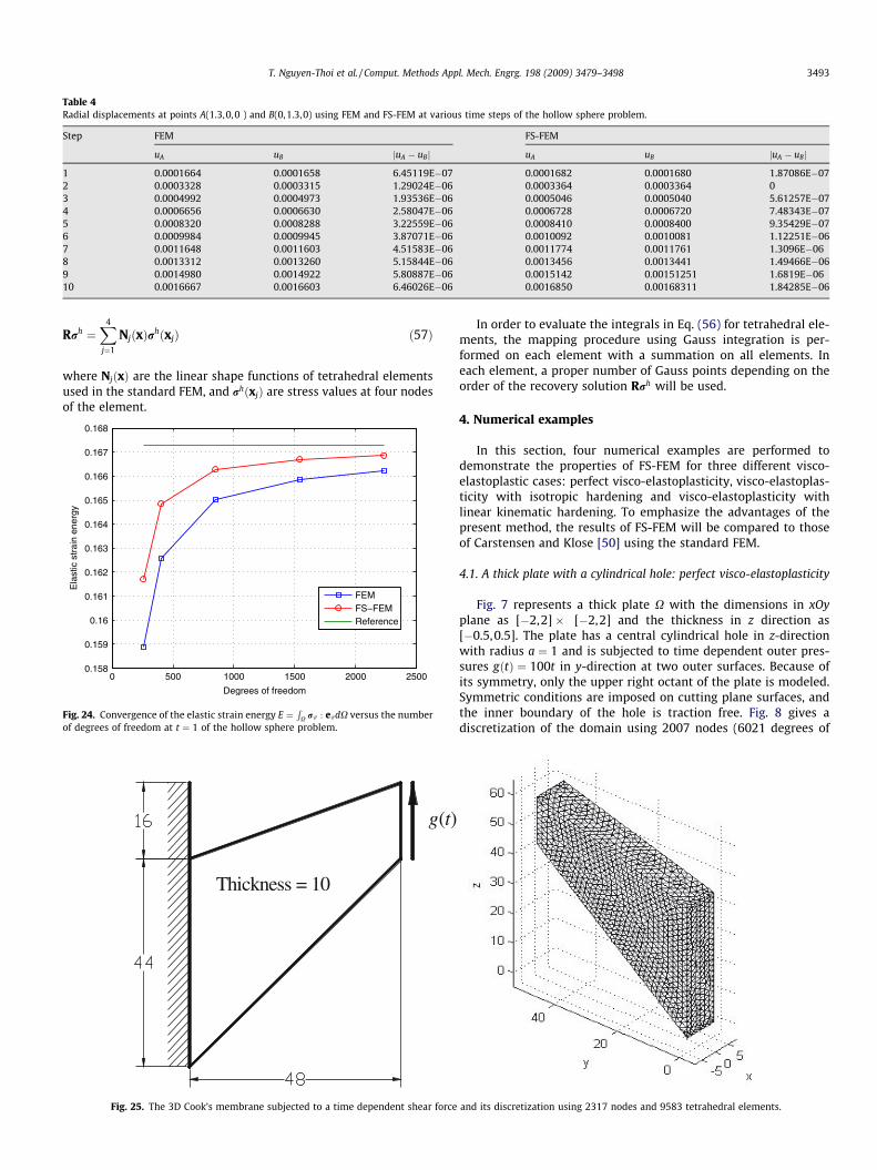
Table 4Radial displacements at points A(1.3,0,0 ) and B(0,1.3,0) using FEM and FS-FEM at various time steps of the hollow sphere problem.

Step FEM FS-FEM

uA uB juA � uBj uA uB juA � uB j

1 0.0001664 0.0001658 6.45119E�07 0.0001682 0.0001680 1.87086E�072 0.0003328 0.0003315 1.29024E�06 0.0003364 0.0003364 03 0.0004992 0.0004973 1.93536E�06 0.0005046 0.0005040 5.61257E�074 0.0006656 0.0006630 2.58047E�06 0.0006728 0.0006720 7.48343E�075 0.0008320 0.0008288 3.22559E�06 0.0008410 0.0008400 9.35429E�076 0.0009984 0.0009945 3.87071E�06 0.0010092 0.0010081 1.12251E�067 0.0011648 0.0011603 4.51583E�06 0.0011774 0.0011761 1.3096E�068 0.0013312 0.0013260 5.15844E�06 0.0013456 0.0013441 1.49466E�069 0.0014980 0.0014922 5.80887E�06 0.0015142 0.00151251 1.6819E�0610 0.0016667 0.0016603 6.46026E�06 0.0016850 0.00168311 1.84285E�06


Rrh ¼X4

j¼1

NjðxÞrhðxjÞ ð57Þ

where NjðxÞ are the linear shape functions of tetrahedral elementsused in the standard FEM, and rhðxjÞ are stress values at four nodesof the element.

Thickness = 10

g(t)

Fig. 25. The 3D Cook’s membrane subjected to a time dependent shear force

0 500 1000 1500 2000 25000.158

0.159

0.16

0.161

0.162

0.163

0.164

0.165

0.166

0.167

0.168

Degrees of freedom

Ela

stic

str

ain

ener

gy



X r# : e#dX versus the numberof degrees of freedom at t ¼ 1 of the hollow sphere problem.

In order to evaluate the integrals in Eq. (56) for tetrahedral ele-ments, the mapping procedure using Gauss integration is per-formed on each element with a summation on all elements. Ineach element, a proper number of Gauss points depending on theorder of the recovery solution Rrh will be used.

4. Numerical examples

In this section, four numerical examples are performed todemonstrate the properties of FS-FEM for three different visco-elastoplastic cases: perfect visco-elastoplasticity, visco-elastoplas-ticity with isotropic hardening and visco-elastoplasticity withlinear kinematic hardening. To emphasize the advantages of thepresent method, the results of FS-FEM will be compared to thoseof Carstensen and Klose [50] using the standard FEM.

4.1. A thick plate with a cylindrical hole: perfect visco-elastoplasticity

Fig. 7 represents a thick plate X with the dimensions in xOyplane as [�2,2] � [�2,2] and the thickness in z direction as[�0.5,0.5]. The plate has a central cylindrical hole in z-directionwith radius a ¼ 1 and is subjected to time dependent outer pres-sures gðtÞ ¼ 100t in y-direction at two outer surfaces. Because ofits symmetry, only the upper right octant of the plate is modeled.Symmetric conditions are imposed on cutting plane surfaces, andthe inner boundary of the hole is traction free. Fig. 8 gives adiscretization of the domain using 2007 nodes (6021 degrees of

and its discretization using 2317 nodes and 9583 tetrahedral elements.

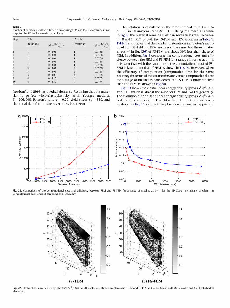
Table 5Number of iterations and the estimated error using FEM and FS-FEM at various timesteps for the 3D Cook’s membrane problem.

Step FEM FS-FEM


Iterations gh ¼ Rrh�rhkL2krhkL2

1 1 0.1101 1 0.07562 1 0.1101 1 0.07563 1 0.1101 1 0.07564 1 0.1101 1 0.07565 1 0.1101 1 0.07566 3 0.1101 3 0.07567 3 0.1101 3 0.07568 3 0.1106 4 0.07589 4 0.1115 4 0.076510 4 0.1130 4 0.0774


freedom) and 8998 tetrahedral elements. Assuming that the mate-rial is perfect visco-elastoplasticity with Young’s modulusE ¼ 206;900, Poisson’s ratio v ¼ 0:29, yield stress rY ¼ 550, andthe initial data for the stress vector ro is set zero.

Fig. 27. Elastic shear energy density kdevðbfRrhÞk2=ð4lÞ for 3D Cook’s membrane probl

elements).

500 1000 1500 2000 2500 3000 3500 4000 4500 5000 55000

500

1000

1500

2000

2500

3000

Degrees of freedom

CP

U ti

me

(sec

onds

)

FEMFS−FEM

a b

Fig. 26. Comparison of the computational cost and efficiency between FEM and FS-Computational cost; and (b) computational efficiency.

The solution is calculated in the time interval from t ¼ 0 tot ¼ 1:0 in 10 uniform steps Dt ¼ 0:1. Using the mesh as shownin Fig. 8, the material remains elastic in seven first steps, betweent ¼ 0 and t ¼ 0:7 for both the FS-FEM and FEM as shown in Table 1.Table 1 also shows that the number of iterations in Newton’s meth-od of both FS-FEM and FEM are almost the same, but the estimatederrors gh in Eq. (56) of FS-FEM are about 30% less than those ofFEM. In addition, Fig. 9 compares the computational cost and effi-ciency between the FEM and FS-FEM for a range of meshes at t ¼ 1.It is seen that with the same mesh, the computational cost of FS-FEM is larger than that of FEM as shown in Fig. 9a. However, whenthe efficiency of computation (computation time for the sameaccuracy) in terms of the error estimator versus computational costfor a range of meshes is considered, the FS-FEM is more efficientthan the FEM as shown in Fig. 9b.

Fig. 10 shows the elastic shear energy density kdevðRrhÞk2=ð4lÞ

at t ¼ 1:0 which is almost the same for FEM and FS-FEM generally.The evolution of the elastic shear energy density kdevðRrhÞk2

=ð4lÞis demonstrated using the FS-FEM at four different time instancesas shown in Fig. 11 in which the plasticity domain first appears at

em using FEM and FS-FEM at t ¼ 1:0 (mesh with 2317 nodes and 9583 tetrahedral

0 1000 2000 3000 4000 5000 60000.06

0.08

0.1

0.12

0.14

0.16

0.18

0.2

0.22

CPU time (seconds)

Est

imat

ed e

rror

ηh

FEMFS−FEM

FEM for a range of meshes at t ¼ 1 for the 3D Cook’s membrane problem. (a)


the corner containing point A(0,1,0.5) and then at the corner con-taining point B(1,0,0.5).

Figs. 12 and 13 show, respectively, the convergence of displace-ments at points A; B and the elastic strain energy E ¼

RX r# : e#dX

versus the number of degrees of freedom at t ¼ 1 by the FEMand FS-FEM. The solution of FS-FEM using a very fine mesh includ-ing 17,991 degrees of freedom and 29,543 elements is used as ref-erence solution. The results show clearly that the FS-FEM model issofter and gives more accurate results than the FEM model usingtetrahedral elements.

4.2. A 3D L-shaped block: perfect visco-elastoplasticity

Consider the 3D square block with a cubic hole subjected to theouter surface traction q as shown in Fig. 14a. Due to the symmetricproperty of the problem, only an eighth of the domain is modeled,which becomes a 3D L-shaped block with the length of 2a for thelong edge, a for the short edge and a=2 for the thickness as shown

Fig. 28. Evolution of the elastic shear energy density kdevðRrhÞk2=ð4lÞ using F

in Fig. 14b. The symmetric conditions are imposed on the cuttingboundary planes. Fig. 15 gives a discretization of the domain using2327 nodes and 10,584 tetrahedral elements. The 3D L-shapedblock is subjected to time dependent outer pressures qðtÞ ¼ 120tin x-direction and the data of length a ¼ 1. Assuming that thematerial is perfect visco-elastoplasticity with Young’s modulusE ¼ 206;900, Poisson’s ratio v ¼ 0:29, yield stress rY ¼ 500, andthe initial data for the stress tensor r0 is set zero.

The solution is calculated in the time interval from t ¼ 0 tot ¼ 1:0 in 10 uniform steps Dt ¼ 0:1. Using the mesh as shown inFig. 15, the material remains elastic in four first steps, betweent ¼ 0 and t ¼ 0:4 for both the FS-FEM and FEM as shown in Table2. Table 2 also shows that the number of iterations in Newton’smethod of both FS-FEM and FEM are the same, but the estimatederrors gh in Eq. (56) of FS-FEM are about 30% less than those ofFEM. In addition, Fig. 16 compares the computational cost and effi-ciency between the FEM and FS-FEM for a range of meshes at t ¼ 1.It is seen that with the same mesh, the computational cost of

S-FEM at some different time steps for the 3D Cook’s membrane problem.

0 1000 2000 3000 4000 5000 6000 7000 80001.06

1.065

1.07

1.075

1.08

1.085

1.09

1.095

1.1

1.105

1.11

Degrees of freedom

Ela

stic

str

ain

ener

gy



X r# : e#dX versus the numberof degrees of freedom at t ¼ 1 of the 3D Cook’s membrane problem.


FS-FEM is larger than that of FEM as shown in Fig. 16a. However,when the efficiency of computation (computation time for thesame accuracy) in terms of the error estimator versus computa-tional cost for a range of meshes is considered, the FS-FEM is moreefficient than the FEM as shown in Fig. 16b.

Fig. 17 shows the elastic shear energy density kdevðRrhÞk2=ð4lÞat t ¼ 1:0 which is also almost the same for the FEM and FS-FEM.The evolution of the elastic shear energy densitykdevðRrhÞk2

=ð4lÞ is demonstrated using the FS-FEM at four differ-ent time instances as shown in Fig. 18 in which the plastic domainfirst appears at the re-entrant corner.

Fig. 19 shows the convergence of the elastic strain energyE ¼

RX r# : e#dX versus the number of degrees of freedom using

the FEM and FS-FEM at t ¼ 1:0. The solution of FS-FEM using a veryfine mesh including 15,390 degrees of freedom and 24,777 ele-ments is used as reference solution. The results again verify thatthe FS-FEM model is softer and gives more accurate results thanthe FEM model using tetrahedral elements.

4.3. The hollow sphere problem: visco-elastoplasticity with isotropichardening

The domain is the hollow sphere X ¼ Bð0;2Þ n Bð0;1:3Þ (the ori-gin Oð0;0;0Þ, inner radius a ¼ 1:3, outer radius b ¼ 2:0Þ subjectedto a uniform pressure gðr;u; tÞ ¼ 50ter on inner radius wither ¼ ðcos u; sin uÞ. Because of the symmetric characteristic of theproblem, only a eighth of hollow sphere is modeled as shown inFig. 20, and symmetric conditions are imposed on the cuttingboundary planes. Assuming that the material is visco-elastoplastic-ity with isotropic hardening with Young’s modulus E ¼ 40;000,Poisson’s ratio v ¼ 0:25, yield stress rY ¼ 100, hardeningparameter H ¼ 3;H1 ¼ 1; and the initial stress vector r0 andthe scalar hardening parameter aI

0 are set zero.The solution is calculated in the time interval from t ¼ 0 to

t ¼ 1:0 in 10 uniform steps Dt ¼ 0:1. Using the mesh as shownin Fig. 20, the material remains elastic in seven first steps, be-tween t ¼ 0 and t ¼ 0:7 for both the FS-FEM and FEM as shownin Table 3. Table 3 also shows that the number of iterations inNewton’s method of both FS-FEM and FEM are almost the same,but the estimated errors gh in Eq. (56) of FS-FEM are about 30%less than those of FEM. In addition, Fig. 21 compares the compu-tational cost and efficiency between the FEM and FS-FEM for arange of meshes at t ¼ 1. It is seen that with the same mesh,the computational cost of FS-FEM is larger than that of FEM asshown in Fig. 21a. However, when the efficiency of computation(computation time for the same accuracy) in terms of the errorestimator versus computational cost for a range of meshes is con-sidered, the FS-FEM is more efficient than the FEM as shown inFig. 21b.


at t ¼ 1:0 which is also almost the same for the FEM and FS-FEM.The evolution of the elastic shear energy densitykdevðRrhÞk2

=ð4lÞ is demonstrated using the FS-FEM at some dif-ferent time instances as shown in Fig. 23 in which the plastic do-main first appears at the inner radius and extents toward theouter radius. Table 4 shows the ratio of radial displacements be-tween points A(1.3,0,0) and B(0,1.3,0) using the FEM and FS-FEMat various time steps. It is seen that for the symmetric problem,the results of FS-FEM is more symmetric than those of FEM.


RX r# : e# dX versus the number of degrees of freedom using


4.4. A 3D Cook’s membrane: visco-elastoplasticity with linearkinematic hardening

Fig. 25 show a 3D Cook’s membrane on yOz plane, and a discret-ization of the domain using 2317 nodes and 9583 tetrahedral ele-ments. At the high end of the membrane, there is a time dependentshear force g ¼ 90tez and the other end is fixed. Assuming that thematerial is visco-elastoplasticity with linear kinematic hardeningwith Young’s modulus E ¼ 70;000, Poisson’s ratio v ¼ 0:3, yieldstress rY ¼ 400, hardening parameter k1 ¼ 2, and the initial datafor the displacement u0, the stress tensor r0 and the hardeningparameter aK

0 are set zero.The solution is calculated in the time interval from t ¼ 0 to

t ¼ 1:0 in 10 uniform steps Dt ¼ 0:1. Using the mesh as shownin Fig. 25, the material remains elastic in five first steps, betweent ¼ 0 and t ¼ 0:5 for both the FS-FEM and FEM as shown in Table5. Table 5 also shows that the number of iterations in Newton’smethod of both the FS-FEM and FEM are almost the same, butthe estimated errors gh in Eq. (56) of FS-FEM are about 30% lessthan those of FEM. In addition, Fig. 26 compares the computa-tional cost and efficiency between the FEM and FS-FEM for arange of meshes at t ¼ 1. It is seen that with the same mesh,the computational cost of FS-FEM is larger than that of FEM asshown in Fig. 26a. However, when the efficiency of computation(computation time for the same accuracy) in terms of the errorestimator versus computational cost for a range of meshes is con-sidered, the FS-FEM is more efficient than the FEM as shown inFig. 26b.


at t ¼ 1:0 which is almost the same for the FEM and FS-FEM. Theevolution of the elastic shear energy density kdevðRrhÞk2

=ð4lÞ isdemonstrated using the FS-FEM at four different time instancesas shown in Fig. 28 in which the plastic domain first appears atthe fixed upper corner and then at the middle part of the lowerboundary face.


RX r# : e#dX versus the number of degrees of freedom using



5. Conclusion

In this paper, the FS-FEM is extended to more complicated vis-co-elastoplastic analyses in 3D solids. We combine the FS-FEMusing tetrahedral elements with the work of Carstensen and Klose[50] in the setting of von-Mises conditions and the Prandtl–Reussflow rule, and the material behavior includes perfect visco-elastoplasticity, and visco-elastoplasticity with isotropic hardeningand linear kinematic hardening in a dual model, with displace-ments and the stresses as the main variables. The numerical proce-dure, however, eliminates the stress variables and the problembecomes only displacement-dependent and is easier to deal with.The numerical results of FS-FEM using tetrahedral elements showthat

� The bandwidth of stiffness matrix of FS-FEM is larger than thatof FEM, and hence the computational cost of FS-FEM is largerthan that of FEM. However, when the efficiency of computation(computation time for the same accuracy) in terms of a posteri-ori error estimation is considered, the FS-FEM is more efficientthan FEM.

� The displacement results of FS-FEM are larger than those of FEM.The elastic strain energy of FS-FEM is more accurate than that ofFEM. These results show clearly that the FS-FEM model canreduce the over-stiffness of the standard FEM model using tetra-hedral elements and gives more accurate results than those ofFEM.

� For the axis-symmetric problems, the results of FS-FEM aremore symmetric than those of FEM.

Acknowledgements

This work is partially supported by A*Star, Singapore. It is alsopartially supported by the Open Research Fund Program of theState Key Laboratory of Advanced Technology of Design andManufacturing for Vehicle Body, Hunan University, P.R.China un-der the grant number 40915001.

References

[1] G.R. Liu, Meshfree Methods: Moving Beyond the Finite Element Method,second ed., Taylor & Francis/CRC Press, Boca Raton, USA, 2009.

[2] G.R. Liu, A G space theory and weakened weak (W2) form for a unifiedformulation of compatible and incompatible methods: part I theory, part IIapplication to solid mechanics problems, Int. J. Numer. Methods Engrg., inpress.

[3] J.S. Chen, C.T. Wu, S. Yoon, Y. You, A stabilized conforming nodal integration forGalerkin meshfree method, Int. J. Numer. Methods Engrg. 50 (2001) 435–466.

[4] J.W. Yoo, B. Moran, J.S. Chen, Stabilized conforming nodal integration in thenatural-element method, Int. J. Numer. Methods Engrg. 60 (2004) 861–890.

[5] G.R. Liu, A generalized gradient smoothing technique and the smoothedbilinear form for Galerkin formulation of a wide class of computationalmethods, Int. J. Comput. Methods 5 (2) (2008) 199–236.

[6] T.P. Fries, H.G. Matthies, Classification and Overview of Meshfree Methods,Institute of Scientific Computing, Technical University Braunschweig,Germany, Informatikbericht.

[7] V.P. Nguyen, T. Rabczuk, Bordas Stephane, M. Duflot, Meshless methods:review and key computer implementation aspects, Math. Comput. Simul. 79(2008) 763–813.

[8] S. Bordas, T. Rabczuk, G. Zi, Three-dimensional crack initiation, propagation,branching and junction in non-linear materials by an extended meshfreemethod without asymptotic enrichment, Eng. Fract. Mech. 75 (5) (2008) 943–960.

[9] T. Rabczuk, T. Belytschko, Cracking particles: a simplified meshfree method forarbitrary evolving cracks, Int. J. Numer. Methods Engrg. 61 (13) (2004) 2316–2343.

[10] T. Rabczuk, T. Belytschko, S.P. Xiao, Stable particle methods based onLagrangian kernels, Comput. Methods Appl. Mech. Engrg. 193 (2004) 1035–1063.

[11] T. Rabczuk, S. Bordas, G. Zi, A three-dimensional meshfree method forcontinuous multiple-crack initiation, propagation and junction in statics anddynamics, Comput. Mech. 40 (3) (2007) 473–495.

[12] T. Rabczuk, T. Belytschko, A three-dimensional large deformation meshfreemethod for arbitrary evolving cracks, Comput. Methods Appl. Mech. Engrg.196 (2007) 2777–2799.

[13] T. Rabczuk, G. Zi, S. Bordas, H. Nguyen-Xuan, A geometrically non-linear three-dimensional cohesive crack method for reinforced concrete structures, Engrg.Fract. Mech. 75 (16) (2008) 4740–4758.

[14] G.R. Liu, G.Y. Zhang, K.Y. Dai, Y.Y. Wang, Z.H. Zhong, G.Y. Li, X. Han, A linearlyconforming point interpolation method (LC-PIM) for 2D solid mechanicsproblems, Int. J. Comput. Methods 2 (4) (2005) 645–665.

[15] G.R. Liu, G.Y. Zhang, Y.Y. Wang, H.T. Huang, Z.H. Zhong, G.Y. Li, X. Han, Alinearly conforming point interpolation method (LC-PIM) for three-dimensional elasticity problems, Int. J. Numer. Methods Engrg. 72 (2007)1524–1543.

[16] G.R. Liu, Y. Li, K.Y. Dai, M.T. Luan, W. Xue, A linearly conforming radial pointinterpolation method for solid mechanics problems, Int. J. Comput. Methods 3(4) (2006) 401–428.

[17] G.R. Liu, K.Y. Dai, T. Nguyen-Thoi, A smoothed finite element method formechanics problems, Comput. Mech. 39 (2007) 859–877.

[18] G.R. Liu, T. Nguyen-Thoi, K.Y. Dai, K.Y. Lam, Theoretical aspects of thesmoothed finite element method (SFEM), Int. J. Numer. Methods Engrg. 71(2007) 902–930.

[19] Hung Nguyen-Xuan, Stéphane Bordas, Hung Nguyen-Dang, Smooth finiteelement methods: convergence, accuracy and properties, Int. J. Numer.Methods Engrg. 74 (2008) 75–208.

[20] G.R. Liu, T. Nguyen-Thoi, H. Nguyen-Xuan, K.Y. Dai, K.Y. Lam, On the essenceand the evaluation of the shape functions for the smoothed finite elementmethod (SFEM) (letter to editor), Int. J. Numer. Methods Engrg. 77 (2009)1863–1869.

[21] G.R. Liu, T. Nguyen-Thoi, H. Nguyen-Xuan, K.Y. Lam, A node-based smoothedfinite element method for upper bound solution to solid problems (NS-FEM),Comput. Struct. 87 (2009) 14–26.

[22] G.R. Liu, T. Nguyen-Thoi, K.Y. Lam, An edge-based smoothed finite elementmethod (ES-FEM) for static, free and forced vibration analyses of solids, J.Sound Vib. 320 (2009) 1100–1130.

[23] H. Nguyen-Xuan, G.R. Liu, T. Nguyen-Thoi, C. Nguyen-Tran, An edge-basedsmoothed finite element method (ES-FEM) for analysis of two-dimensionalpiezoelectric structures, Smart Mater. Struct. 18 (2009) 065015. 12p.

[24] T. Nguyen-Thoi, G.R. Liu, H.C. Vu-Do, H. Nguyen-Xuan, An edge-basedsmoothed finite element method (ES-FEM) for visco-elastoplastic analyses in2D solids mechanics using triangular mesh, Comput. Mech., 2009, in press.

[25] H. Nguyen-Xuan, G.R. Liu, C. Thai-Hoang, T. Nguyen-Thoi, An edge-basedsmoothed finite element method with stabilized discrete shear gap techniquefor analysis of Reissner–Mindlin plates, Comput. Methods Appl. Mech. Engrg.,2009, submitted for publication.

[26] Thanh Ngoc Tran, G.R. Liu, H. Nguyen-Xuan, T. Nguyen-Thoi, An edge-basedsmoothed finite element method for primal-dual shakedown analysis ofstructures, Int. J. Numer. Methods Engrg., 2009 (Revised).

[27] S.P. A Bordas, T. Rabczuk, N.X. Hung, V.P. Nguyen, S. Natarajan, T. Bog, D.M.Quan, N.V. Hiep, Strain smoothing in FEM and XFEM, Comput. Struct. (2009),doi:10.1016/j.compstruc.2008.07.006.

[28] K.Y. Dai, G.R. Liu, T. Nguyen-Thoi, An n-sided polygonal smoothed finiteelement method (nSFEM) for solid mechanics, Finite Elements Anal. Des. 43(2007) 847–860.

[29] K.Y. Dai, G.R. Liu, Free and forced analysis using the smoothed finite elementmethod (SFEM), J. Sound Vib. 301 (2007) 803–820.

[30] T. Nguyen-Thoi, G.R. Liu, K.Y. Dai, K.Y. Lam, Selective smoothed finite elementmethod, Tsinghua Sci. Technol. 12 (5) (2007) 497–508.

[31] H. Nguyen-Xuan, S. Bordas, H. Nguyen-Dang, Addressing volumetric lockingand instabilities by selective integration in smoothed finite elements,Commun. Numer. Methods Engrg. 25 (2008) 19–34.

[32] H. Nguyen-Xuan, T. Nguyen-Thoi, A stabilized smoothed finite elementmethod for free vibration analysis of Mindlin–Reissner plates, Commun.Numer. Methods Eng. 25 (2009) 882–906.

[33] X.Y. Cui, G.R. Liu, G.Y. Li, X. Zhao, T. Nguyen-Thoi, G.Y. Sun, A smoothed finiteelement method (SFEM) for linear and geometrically nonlinear analysis ofplates and shells, CMES – Comput. Model. Engrg. Sci. 28 (2) (2008) 109–125.

[34] N. Nguyen-Thanh, T. Rabczuk, H. Nguyen-Xuan, S. Bordas, A smoothed finiteelement method for shell analysis, Comput. Methods Appl. Mech. Engrg. 198(2008) 165–177.

[35] H. Nguyen-Van, N. Mai-Duy, T. Tran-Cong, A smoothed four-node piezoelectricelement for analysis of two-dimensional smart structures, CMES – Comput.Model. Eng. Sci. 23 (3) (2008) 209–222.

[36] H. Nguyen-Xuan, T. Rabczuk, S. Bordas, J.F. Debongnie, A smoothed finiteelement method for plate analysis, Comput. Methods Appl. Mech. Engrg. 197(2008) 1184–1203.

[37] S. Bordas, T. Rabczuk, H. Nguyen-Xuan, P. Nguyen Vinh, S. Natarajan, T. Bog, Q.Do Minh, H. Nguyen Vinh, Strain smoothing in FEM and XFEM, Comput. Struct.(2009), doi:10.1016/j.compstruc.2008.07.006.

[38] N. Sukumar, E.A. Malsch, Recent advances in the construction of polygonalfinite element interpolants, Arch. Comput. Methods Engrg. 13 (1) (2006) 129–163.

[39] N. Sukumar, A. Tabarraei, Conforming polygonal finite elements, Int. J. Numer.Methods Engrg. 61 (2004) 2045–2066.

[40] N. Sukumar, Construction of polygonal interpolants: a maximum entropyapproach, Int. J. Numer. Methods Eng. 61 (2004) 2159–2181.

http://dx.doi.org/10.1016/j.compstruc.2008.07.006

http://dx.doi.org/10.1016/j.compstruc.2008.07.006


[41] S. Natarajan, S. Bordas, D.R. Mahapatra, Numerical integration over arbitrarypolygonal domains based on Schwarz–Christoffel conformal mapping, Int. J.Numer. Methods Eng. (2009), doi:10.1002/nme.

[42] C.R. Dohrmann, M.W. Heinstein, J. Jung, S.W. Key, W.R. Witkowski, Node-baseduniform strain elements for three-node triangular and four-node tetrahedralmeshes, Int. J. Numer. Methods Engrg. 47 (2000) 1549–1568.

[43] G.R. Liu, G.Y. Zhang, Upper bound solution to elasticity problems: a uniqueproperty of the linearly conforming point interpolation method (LC-PIM), Int. J.Numer. Methods Engrg. 74 (2008) 1128–1161.

[44] G.R. Liu, T. Nguyen-Thoi, K.Y. Lam, A novel alpha finite element method (aFEM)for exact solution to mechanics problems using triangular and tetrahedralelements, Comput. Methods Appl. Mech. Engrg. 197 (2008) 3883–3897.

[45] A.J. Aref, Z. Guo, Framework for finite-element-based large increment methodfor nonlinear structural problems, J. Engrg. Mech. 127 (2001) 739–746.

[46] S.N. Patnak, The integrated force method versus the standard force method,Comput. Struct. 22 (1986) 151–163.

[47] B.F. Veubeke, Displacement and equilibrium models in the finite elementmethod, in: O.C. Zienkiewicz, G.S. Holister (Eds.), Stress Analysis, Wiley,London, 1965.

[48] T. Nguyen-Thoi, G.R. Liu, H. Nguyen-Xuan, C. Nguyen-Tran, Adaptive analysisusing the node-based smoothed finite element method (NS-FEM), Commun.Numer. Methods Engrg. (2009), doi:10.1002/cnm.1291.

[49] T. Nguyen-Thoi, G.R. Liu, K.Y. Lam, G.Y. Zhang, A face-based smoothed finiteelement method (FS-FEM) for 3D linear and nonlinear solid mechanics

problems using 4-node tetrahedral elements, Int. J. Numer. Methods Engrg.78 (2009) 324–353.

[50] C. Carstensen, R. Klose, Elastoviscoplastic finite element analysis in 100 lines ofmatlab, J. Numer. Math. 10 (2002) 157–192.

[51] C. Carstensen, S.A. Funken, Averaging technique for FE-a posteriori errorcontrol in elasticity. Part 1: conforming FEM, Comput. Methods Appl. Mech.Engrg. 190 (2001) 2483–2498.

[52] M. Duflot, S. Bordas, A posteriori error estimation for extended finite elementsby an extended global recovery, Int. J. Numer. Methods Engrg. 76 (2008) 1123–1138.

[53] S. Bordas, M. Duflot, Derivative recovery and a posteriori error estimate forextended finite elements, Comput. Methods Appl. Mech. Engrg. 196 (2007)3381–3399.

[54] S. Bordas, M. Duflot, P. Le, A simple error estimator for extended finiteelements, Commun. Numer. Methods Engrg. 24 (2008) 961–971.

[55] J.J. Rodenas, O.A. Gonzalez-Estrada, J.E. Tarancon, F.J. Fuenmayor, A recovery-type error estimator for the extended finite element method based onsingular + smooth stress field splitting, Int. J. Numer. Methods Engrg. 76(2008) 545–571.

[56] T. Rabczuk, T. Belytschko, Adaptivity for structured meshfree particle methodsin 2D and 3D, Int. J. Numer. Methods Engrg. 63 (2005) 1559–1582.

[57] T. Pannachet, L.J. Sluys, H. Askes, Error estimation and adaptivityfor discontinuous failure, Int. J. Numer. Methods Engrg. 78 (2008) 528–563.

http://dx.doi.org/10.1002/nme

http://dx.doi.org/10.1002/cnm.1291

Date post:	29-May-2018
Category:	Documents
Upload:	phamnga
View:	214 times
Download:	0 times

Comput. Methods Appl. Mech. Engrg. - University of Cincinnatiliugr/Publications/Journal...

Documents