Comput. Methods Appl. Mech. Engrg. - Weierstrass … element methods for time-dependent...

Comput. Methods Appl. Mech. Engrg. 198 (2008) 475–494

Contents lists available at ScienceDirect

Comput. Methods Appl. Mech. Engrg.

journal homepage: www.elsevier .com/locate /cma

Finite element methods for time-dependent convection–diffusion–reactionequations with small diffusion

Volker John *, Ellen Schmeyer 1

FR 6.1 – Mathematik, Universität des Saarlandes, Postfach 15 11 50, 66041 Saarbrücken, Germany

a r t i c l e i n f o a b s t r a c t

Article history:Received 14 May 2008Received in revised form 25 August 2008Accepted 28 August 2008Available online 12 September 2008

Keywords:Time-dependent convection–diffusion–reaction equationsFinite element methodsSmall diffusion parameterSpurious oscillations

0045-7825/$ - see front matter � 2008 Elsevier B.V. Adoi:10.1016/j.cma.2008.08.016

* Corresponding author. Tel.: +49 681 302 4445; faE-mail addresses: [email protected] (V. John

(E. Schmeyer).1 The research of E. Schmeyer was supported by th

inschaft (DFG) by Grant No. Jo 329/8-1.

Numerical studies of stabilized finite element methods for solving scalar time-dependent convection–dif-fusion–reaction equations with small diffusion are presented in this paper. These studies include thestreamline-upwind Petrov–Galerkin (SUPG) method with different parameters, various spurious oscilla-tions at layers diminishing (SOLD) methods, a local projection stabilization (LPS) scheme based on enrich-ment and two finite element method flux corrected transport (FEM-FCT) methods. The focus of theevaluation of the numerical results is on the reduction of spurious oscillations.

� 2008 Elsevier B.V. All rights reserved.

1. Introduction

The simulation of time-dependent convection–diffusion–reac-tion equations is required in various applications. A typical exam-ple is the simulation of processes which involve a chemicalreaction in a flow field. Such reactions are modeled by a non-linearsystem of time-dependent convection–diffusion–reaction equa-tions for the concentrations of the reactants and the products.These equations are strongly coupled such that inaccuracies inone concentration directly affect all other concentrations. Typi-cally, the size of the diffusion is smaller by several orders of mag-nitude compared to the size of the flow field. That means, theconvection–diffusion–reaction equations are convection-domi-nated. Often, there is also a strong chemical reaction such thatthe equations become reaction-dominated, too. A characteristicfeature of solutions of convection- and reaction-dominated equa-tions is the presence of sharp layers. The accurate simulation ofsuch processes requires numerical methods which are, on theone hand, able to compute sharp layers and which prevent, onthe other hand, the occurrence of spurious oscillations.

A special example of processes with chemical reactions in a flowfield are precipitation processes. In [39], a calcium carbonate pre-cipitation was simulated, where the system of time-dependent

ll rights reserved.

x: +49 681 302 3046.), [email protected]

e Deutsche Forschungsgeme-

convection–diffusion–reaction equations was discretized in timewith the Crank–Nicolson scheme and in space with the Q1 finiteelement method. Since the equations in the system are convection-and reaction-dominated, a stabilization of the finite element dis-cretization is necessary. In [39], the standard streamline-upwindPetrov–Galerkin (SUPG) method [30,7] with the parameter from[49] was used. This approach led to computed concentrations withconsiderable spurious oscillations, see Fig. 1 for an illustration. Inthe simulations presented in [39], which use laminar flow fieldsin 2D, negative oscillations (negative concentrations) were justcut off. We could observe in further numerical tests that increasingthe Reynolds number of the flow fields in 2D or performing simu-lations in 3D (on coarser grids) led to a piling up of the remainingpositive oscillations and finally to a blow-up of the simulations.Likewise, in [39] is reported that the use of a very diffusive upwindscheme led to unphysical results. Hence, there is the need of bettermethods, namely methods which fulfill the two requirements gi-ven above.

The first step in identifying appropriate methods for the accu-rate simulation of the chemical reaction process is of course theconsideration of scalar time-dependent convection–diffusion–reaction equations. The code which is used for the simulation ofthe precipitation process is based on finite element methods. Wewill concentrate in this paper on first order finite elements, whichare the simplest and most often used finite elements.

A study of stabilized finite element methods for time-depen-dent convection–diffusion–reaction equations can be found in[14]. This study clarified similarities and differences between sev-eral methods, among them the SUPG method. The basic idea in the

mailto:[email protected]

mailto:[email protected]

http://www.sciencedirect.com/science/journal/00457825

http://www.elsevier.com/locate/cma

Fig. 1. Spurious oscillations of a concentration in the simulation of a precipitationprocess computed with the SUPG method.

476 V. John, E. Schmeyer / Comput. Methods Appl. Mech. Engrg. 198 (2008) 475–494

application of stabilized finite element methods is that after thetemporal discretization of the time-dependent equation, the equa-tion has the form of a steady-state convection–diffusion–reactionequation. Appropriate parameters for the SUPG method appliedto steady-state convection–diffusion–reaction equations have beenstudied in [15] and for the unusual stabilized finite element meth-od (USFEM) in [20]. Steady-state convection–diffusion–reactionequations with positive and negative reactive terms (source terms)were considered in [26]. A non-linear extension of the SUPG ap-proach which tries to reduce spurious oscillations, which is similarto the SOLD method KLR02 in the present paper, was analyzed in[42]. The analysis was extended to higher order finite elements,taking the polynomial degree into account, in [49]. Finite elementmethods for time-dependent convection–diffusion–reaction equa-tions which are based on variational multiscale principles wereconsidered e.g. in [16,27,33,24].

Since it has been known for a long time that the SUPG methodleads to solutions with spurious oscillations also for steady-stateconvection–diffusion equations, several methods have been pro-posed to reduce or to remove these oscillations. These methodsare called Spurious Oscillations at Layers Diminishing (SOLD)methods, see [34,36] for a review. However, very few of them havebeen so far used in the simulation of time-dependent equations,see [2] for an example.

In recent years, local projection stabilization (LPS) schemeshave been developed for stabilizing convection-dominated prob-lems [3,5,6]. A scheme of this type was used for the computationof steady-state convection–diffusion equations in [50]. We arenot aware that LPS schemes were applied already in the simulationof time-dependent convection–diffusion–reaction equations.

All approaches mentioned so far try to stabilize the finite ele-ment method by adding additional terms to the Galerkin finite ele-ment discretization. A different approach are finite elementmethod flux corrected transport (FEM-FCT) schemes[46,45,44,43]. These schemes work on the algebraic level, thatmeans they modify the algebraic equation which is obtained fromthe Galerkin finite element method. Roughly speaking, this equa-tion is firstly replaced with an equation representing a low orderscheme which introduces too much diffusion. Then, the diffusionis removed again in regions where it is not needed by modifyingthe right hand side. The modifications are based on an auxiliarysolution which is computed with a non-oscillatory explicit scheme.

This paper presents first steps in identifying appropriate finiteelement methods for the simulation of scalar time-dependent con-vection–diffusion–reaction equations. Many of the available meth-ods, like SUPG methods with different parameters, various SOLDmethods, a LPS scheme and two FEM-FCT methods are comparednumerically. To our best knowledge, many of these methods have

not yet been used in the simulation of time-dependent problems sofar. In addition, it seems to be the first comparison of FEM-FCTmethods to more traditional schemes for the stabilization of finiteelement methods of convection-dominated and reaction-domi-nated equations. The main goal of the paper consists in identifyingthose methods which show the capability to improve the solutionobtained with the SUPG method considerably.

The paper is organized as follows. Section 2 presents the equa-tions, the temporal discretization and introduces notations. In Sec-tion 3, the SUPG method is described and available proposals forthe parameter are reviewed. Section 4 is devoted to the descriptionof the SOLD methods. The LPS scheme will be introduced in Section5 and the FEM-FCT schemes in Section 6. Section 7 contains thenumerical studies and the evaluation of the methods. The conclu-sions are summarized in Section 8.

2. Basic discretizations

Throughout the paper, we use the standard notations LpðXÞ forLebesgue spaces and Wk;pðXÞ, HkðXÞ ¼Wk;2ðXÞ for Sobolev spaces.The inner product in the space L2ðXÞ will be denoted by ð�; �Þ. Fora vector b 2 Rd, the symbol kbk2 stands for its Euclidean norm.

We consider the scalar convection–diffusion–reaction equation

ut � eDuþ b � ruþ cu ¼ f in ð0; T� �X; ð1Þ

where e > 0 is the diffusion coefficient, b 2 L1ð0; T; W1;1ðXÞÞd is theconvection field with r � b ¼ 0, c 2 L1ð0; T; L1ðXÞÞ is the non-nega-tive reaction coefficient, f 2 L2ð0; T; L2ðXÞÞ, T > 0 is the final timeand X � Rd, d 2 f2;3g, is a bounded domain. This equation has tobe equipped with appropriate boundary conditions and an initialcondition u0 ¼ uð0;xÞ.

We will consider fractional-step h-schemes as temporal discret-ization of (1). These schemes applied to (1) lead at the discretetime tk to an equation of the form

uk þ h1Dtkð�eDuk þ b � ruk þ cukÞ¼ uk�1 � h2Dtkð�eDuk�1 þ b � ruk�1 þ cuk�1Þþ h3Dtkfk�1 þ h4Dtkfk ð2Þ

with Dtk ¼ tk � tk�1 and the parameters h1; . . . ; h4. The backward Eu-ler scheme is obtained for h1 ¼ h4 ¼ 1, h2 ¼ h3 ¼ 0 and the Crank–Nicolson scheme for h1 ¼ h2 ¼ h3 ¼ h4 ¼ 0:5. Eq. (2) can be consid-ered as a stationary convection–diffusion–reaction equation at tk

with the diffusion, convection and reaction, respectively, given by

D ¼ h1Dtke; ð3ÞC ¼ h1Dtkb; ð4ÞR ¼ 1þ h1Dtkc: ð5Þ

Eq. (2) will be discretized with a finite element method. To applysuch a method, (2) can be transformed into a weak formulation inthe usual way by multiplying with test functions from an appropri-ate space V and applying integration by parts. Finite element meth-ods employ now a finite dimensional space Vh instead of V. Forsimplicity of presentation, homogeneous Dirichlet conditions andconforming finite elements, Vh � V , are considered. A Galerkin finiteelement problem arising from (2) reads as follows: Find uh

k 2 Vh

such that

ðuhk ;

hÞ þ h1Dtkððeruhk ;rhÞ þ ðb � ruh

k þ cuhk ;

hÞÞ¼ ðuh

k�1;hÞ � h2Dtkððeruh

k�1;rhÞ þ ðb � ruhk�1 þ cuh

k�1;hÞÞ

þ h3Dtkðfk�1;hÞ þ h4Dtkðfk;

hÞ ð6Þ

for all h 2 Vh. The definition of Vh is usually based on an underlyingtriangulation Th of X. We assume that this triangulation fulfills theusual compatibility conditions, see [12].

V. John, E. Schmeyer / Comput. Methods Appl. Mech. Engrg. 198 (2008) 475–494 477

It is well known that in the case of dominant convection or reac-tion, the Galerkin finite element formulation becomes instable andthe solution of (6) shows spurious oscillations in the wholedomain.

3. The SUPG method

3.1. The general approach

A popular finite element stabilization method for convection-dominated problems is the streamline-upwind Petrov–Galerkin(SUPG) method [30,7], which adds a consistent diffusion term instreamline directionXK2Th

sK ðresidual of ð2Þ;C � rvhÞK ð7Þ

to (6), where fsKg is a set of parameters depending on the meshcells K 2Th, ð�; �ÞK is the inner product in L2ðKÞ and C denotes theconvection. The residual is defined by the difference of the left handside and the right hand side of (2).

Inserting (7) into (6), using the convection given by (4) andrearranging terms lead to

ðuhk ; v

hÞ þX

K2Th

ðsKh1DtkÞðuk;b � rvhÞK

þ h1Dtk

"ðeruh

k ;rvhÞ þ ðb � ruhk þ cuh

k ; vhÞ

þX

K2Th

ðsKh1DtkÞðð�eDuk þ b � ruk þ cukÞ;b � rvhÞK

#

¼ ðuhk�1; v

hÞ þX

K2Th

ðsKh1DtkÞðuk�1;b � rvhÞK

� h2Dtk

"ððeruh

k�1;rvhÞ þ ðb � ruhk�1 þ cuh

k�1; vhÞÞ

þX

K2Th

ðsKh1DtkÞðð�eDuk�1 þ b � ruk�1 þ cuk�1Þ;b � rvhÞK

#

þ h3Dtk ðfk�1; vhÞ þX

K2Th

ðsKh1DtkÞðDtkfk�1;b � rvhÞK

" #

þ h4Dtk ðfk; vhÞ þX

K2Th

ðsKh1DtkÞðDtkfk;b � rvhÞK

" #: ð8Þ

3.2. Proposals for the parameter

The crucial question in the application of the SUPG stabilizationis of course the choice of the parameters fsKg. There is a largeamount of literature concerning this choice in the case that thereaction term is absent. However, for the time-dependent convec-tion–diffusion–reaction equations, the reaction (5) might dominatethe diffusion (3) and the convection (4), in particular for small timesteps. Thus, appropriate parameters should take the reaction intoaccount, see also the numerical studies in Example 7.1. There areseveral proposals in the literature for such parameters. Let D;C;Rbe the abbreviations for diffusion, convection and reaction, respec-tively, where we are interested in particular in the expressionsgiven in (3)–(5).

In [15], it was proposed to set the parameter on the mesh cell Kto be

sCodK � 4jDj

h2K

þ 2kbk2

hKþ jRj

!�1

which gives for (3)–(5)

sCodK � h2

K

4h1Dtkeþ 2hKh1Dtkkbk2 þ h2Kð1þ h1DtkcÞ

: ð9Þ

Here, hK is an appropriate measure for the size of the mesh cell K.Note that sK depends in general on the point x 2 K.

In [20], the parameter

sFVK �

h2K

jRjh2KnðPeK;1Þ þ ð2jDj=mKÞnðPeK;2Þ

with

PeK;1 ¼2jDj

mK jRjh2K

; PeK;2 ¼mKkCk2hK

jDj ; nðjÞ ¼1 0 6 j 6 1;j j P 1

�

was proposed for the unusual finite element method (USFEM). Thisparameter was used in the SUPG method in [26]. The parameter mK

comes from an inverse estimate. For linear finite elements, it ismK ¼ 1=3, which holds in practice also for bilinear finite elements[26]. Inserting (3)–(5) gives

sFVK �

h2K

ð1þ h1DtkcÞh2KnðPeK;1Þ þ 6h1DtkenðPeK;2Þ

ð10Þ

with

PeK;1 ¼6h1Dtke

h2Kð1þ h1DtkcÞ

; PeK;2 ¼hKh1Dtkkbk2

3h1Dtke¼ hKkbk2

3e:

The appropriate measure of the mesh cell hK is also discussed in[20]. It is proposed to set hK as the diameter of the mesh cell inthe direction of the convection, see also [34] for a discussion of thistopic.

In [42,49], it is proposed to set

sKLRK �min

hK

pKkCkL1ðKÞ;

1kRkL1ðKÞ

;h2

K

p4K c2

invkDkL1ðKÞ

( );

where pK is the polynomial degree of the finite element in the meshcell K and cinv is a constant from an inverse estimate. We consider(bi-)linear finite elements, i.e. pK ¼ 1 and cinv ¼ 1. From the compu-tational point of view, it is easier to replace the norms in L1ðKÞ bythe norms which are used in the other proposals of the stabilizationparameter. Thus, we consider

sKLRK �min

hK

2kCk2;

1jRj ;

h2K

jDj

( );

where also the factor 1=2 was introduced in the first term, see thediscussion below of some limit cases for the different parameters.Inserting (3)–(5) leads to

sKLRK �min

hK

2h1Dtkkbk2;

11þ h1Dtkc

;h2

K

h1Dtke

( ): ð11Þ

It turns out that all three proposals of the parameters givesimilar results in some interesting limit cases. Consider first theconvection-dominated regime, where the local Péclet number islarge

PeK ¼kbk2hK

2e� 1

with kbk2 ¼ Oð1Þ from which follows e hK . If Dtk hK 1, thenone obtains

sCodK � sFV

K � sKLRK � 1

1þ h1Dtkc;

0.05 0.1 0.15 0.2 0.250.98

0.985

0.99

0.995

1

τ K

CodinaFranca/ValentinKnopp/Lube/Rapin

Δ tk

Fig. 3. SUPG parameters sCodK ; sFV

K ; sKLRK for e ¼ 10�6, kbk2 ¼ 10�3, c ¼ 0, h1 ¼ 0:5 and

hK ¼ 1=64.


where PeK;1 < 1 in the definition of sFVK . This case is of interest if fast

reactive processes are modeled, whose numerical simulationrequires the use of a small time scale. Another case which might oc-cur often in applications is Dtk � hK 1. This gives

sCodK � sFV

K �hK

2h1Dtkkbk2 þ hKð1þ h1DtkcÞ ;

sKLRK �min

hK

2h1Dtkkbk2;

11þ h1Dtkc

� �:

Clearly, if � is replaced by ¼, then sKLRK P sCod

K ; sFVK in this case. The

ratio sKLRK =sCod

K depends on all inputs in the definition of the param-eters. Fig. 2 shows that sKLR

K might be considerably larger than theother parameters. Very similar pictures as in this figure are obtainedfor c ¼ 0.

In applications like in [39], the convection field b is often avelocity field which was computed by solving the Navier–Stokesequations numerically. This velocity field might have regionswhere kbk2 is small and generally c is small in these regions, too.Considering the limit kbk2 ! 0, c ¼ 0, one obtains for the parame-ters, in the case h2

K � Dtke,

sCodK � sFV

K � sKLRK ! 1;

see also Fig. 3. Since the SUPG term vanishes for kbk2 ! 0, thus itvanishes in the same way for all stabilization parameters.

Remark. The appropriate measure of the mesh cell hK should bechosen as the length of the mesh cell in the direction of theconvection for scalar convection–diffusion equations [53,20,34].This choice is recommended also in the case of steady-stateconvection–diffusion–reaction equations in [20]. However, it is notclear if this remains the appropriate choice if the reactiondominates convection very strongly as in the case of time-dependent equations with small time steps. The contribution ofthe reaction R will dominate all parameters in this case. This termdoes not involve the mesh size and thus the actual choice of hK is ofminor importance. In fact, numerical studies (not presented here)showed that one obtains almost identical results as presented inSection 7 if hK is simply chosen to be the diameter of the mesh cellK.

Remark. The stability of the SUPG method applied to time-depen-dent convection–diffusion equations was studied analytically in[4]. It was proven that the coupling of the SUPG method to implicittime stepping schemes leads to a stable discretization, regardlessof the length of the time step. In addition, it is pointed out that spu-rious oscillations may be expected for small time steps, which canbe observed also in the numerical studies presented in [4] and inSection 7.

0.05 0.1 0.15 0.2 0.25

0.1

0.2

0.3

0.4

0.5

0.6

0.7

0.8

0.9

1

τ K

CodinaFranca/ValentinKnopp/Lube/Rapin

Δ tk

Fig. 2. SUPG parameters sCodK ; sFV

K ; sKLRK for e ¼ 10�6, kbk2 ¼ 1, c ¼ 1, h1 ¼ 0:5 and hK ¼ 1=64

4. SOLD methods

SOLD methods have been developed to reduce or even to re-move spurious oscillations at layers from SUPG finite element solu-tions of steady-state scalar convection–diffusion equations. Onecan distinguish several classes of SOLD methods, see the reviews[34,36]. These reviews reveal that currently there is no SOLDmethod which generally works satisfactorily. Some of the SOLDmethods improve the results of the SUPG discretization consider-ably in special examples. But in [34–36], for each SOLD methodexamples were found where it fails.

Most of the SOLD methods were derived for equations with con-vection and diffusion but without reactive term. There are only fewexamples in which SOLD methods were used for the simulation oftime-dependent problems [2].

In the numerical studies presented in Section 7, a number of SOLDmethods which have been studied for steady-state equations in [34–36] will be used in the simulation of time-dependent convection–diffusion–reaction equations. These studies should give first impres-sions on the effect of the SOLD methods in equations of this kind andthey should provide hints for improving the methods.

The numerical studies in Section 7 investigate SOLD methodswhich add isotropic diffusion

ð~eruhk ;rvhÞ; ð12Þ

SOLD methods which add anisotropic diffusion (orthogonal to thestreamlines)

0.05 0.1 0.15 0.2 0.251

1.2

1.4

1.6

1.8

2

KKLR

/KC

od

Δ tk

ττ

. The curves of sCodK , and sFV

K are on top of each other. Right picture: ratio of sKLRK and sCod

K .


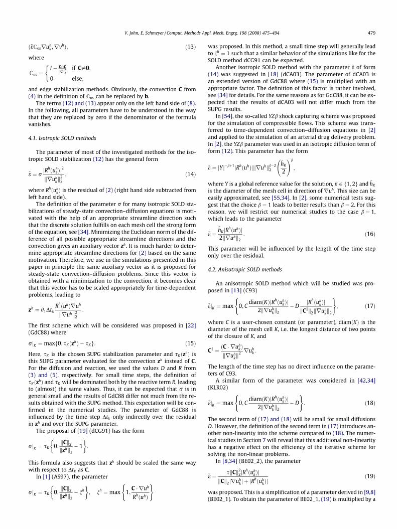
ð~eCosruhk ;rvhÞ; ð13Þ

where

Cos ¼I � CC

kCk22

if C–0;

0 else;

(

and edge stabilization methods. Obviously, the convection C from(4) in the definition of Cos can be replaced by b.

The terms (12) and (13) appear only on the left hand side of (8).In the following, all parameters have to be understood in the waythat they are replaced by zero if the denominator of the formulavanishes.

4.1. Isotropic SOLD methods

The parameter of most of the investigated methods for the iso-tropic SOLD stabilization (12) has the general form

~e ¼ rjRhðuh

kÞj2

kruhkk

22

; ð14Þ

where RhðuhkÞ is the residual of (2) (right hand side subtracted from

left hand side).The definition of the parameter r for many isotropic SOLD sta-

bilizations of steady-state convection–diffusion equations is moti-vated with the help of an appropriate streamline direction suchthat the discrete solution fulfills on each mesh cell the strong formof the equation, see [34]. Minimizing the Euclidean norm of the dif-ference of all possible appropriate streamline directions and theconvection gives an auxiliary vector zh. It is much harder to deter-mine appropriate streamline directions for (2) based on the samemotivation. Therefore, we use in the simulations presented in thispaper in principle the same auxiliary vector as it is proposed forsteady-state convection–diffusion problems. Since this vector isobtained with a minimization to the convection, it becomes clearthat this vector has to be scaled appropriately for time-dependentproblems, leading to

zh ¼ h1DtkRhðuhÞruh

kruhk22

:

The first scheme which will be considered was proposed in [22](GdC88) where

rjK ¼maxf0; sKðzhÞ � sKg: ð15Þ

Here, sK is the chosen SUPG stabilization parameter and sKðzhÞ isthis SUPG parameter evaluated for the convection zh instead of C.For the diffusion and reaction, we used the values D and R from(3) and (5), respectively. For small time steps, the definition ofsKðzhÞ and sK will be dominated both by the reactive term R, leadingto (almost) the same values. Thus, it can be expected that r is ingeneral small and the results of GdC88 differ not much from the re-sults obtained with the SUPG method. This expectation will be con-firmed in the numerical studies. The parameter of GdC88 isinfluenced by the time step Dtk only indirectly over the residualin zh and over the SUPG parameter.

The proposal of [19] (dCG91) has the form

rjK ¼ sK 0;kCk2

kzhk2� 1

� �:

This formula also suggests that zh should be scaled the same waywith respect to Dtk as C.

In [1] (AS97), the parameter

rjK ¼ sK 0;kCk2

kzhk2� nh

� �; nh ¼max 1;

C � ruh

RhðuhÞ

( )

was proposed. In this method, a small time step will generally leadto nh ¼ 1 such that a similar behavior of the simulations like for theSOLD method dCG91 can be expected.

Another isotropic SOLD method with the parameter ~e of form(14) was suggested in [18] (dCA03). The parameter of dCA03 isan extended version of GdC88 where (15) is multiplied with anappropriate factor. The definition of this factor is rather involved,see [34] for details. For the same reasons as for GdC88, it can be ex-pected that the results of dCA03 will not differ much from theSUPG results.

In [54], the so-called YZb shock capturing scheme was proposedfor the simulation of compressible flows. This scheme was trans-ferred to time-dependent convection–diffusion equations in [2]and applied to the simulation of an arterial drug delivery problem.In [2], the YZb parameter was used in an isotropic diffusion term ofform (12). This parameter has the form

~e ¼ jYj�bþ1jRhðuhÞjkruhkb�22

~hK

2

!b

;

where Y is a global reference value for the solution, b 2 f1;2g and ~hK

is the diameter of the mesh cell in direction ofruh. This size can beeasily approximated, see [55,34]. In [2], some numerical tests sug-gest that the choice b ¼ 1 leads to better results than b ¼ 2. For thisreason, we will restrict our numerical studies to the case b ¼ 1,which leads to the parameter

~e ¼~hK jRhðuhÞj2kruhk2

: ð16Þ

This parameter will be influenced by the length of the time steponly over the residual.

4.2. Anisotropic SOLD methods

An anisotropic SOLD method which will be studied was pro-posed in [13] (C93)

~ejK ¼max 0;CdiamðKÞjRhðuh

kÞj2kruh

kk2

� DjRhðuh

kÞjkCkk2kruh

kk2

( ); ð17Þ

where C is a user-chosen constant (or parameter), diamðKÞ is thediameter of the mesh cell K, i.e. the longest distance of two pointsof the closure of K, and

Ck ¼ ðC � ruhkÞ

kruhkk

2 ruhk :

The length of the time step has no direct influence on the parame-ters of C93.

A similar form of the parameter was considered in [42,34](KLR02)

~ejK ¼max 0;CdiamðKÞjRhðuh

kÞj2kruh

kk2

� D

( ): ð18Þ

The second term of (17) and (18) will be small for small diffusionsD. However, the definition of the second term in (17) introduces an-other non-linearity into the scheme compared to (18). The numer-ical studies in Section 7 will reveal that this additional non-linearityhas a negative effect on the efficiency of the iterative scheme forsolving the non-linear problems.

In [8,34] (BE02_2), the parameter

~e ¼ skCk22jR

hðuhkÞj

kCk2jruhk j þ jR

hðuhkÞj

ð19Þ

was proposed. This is a simplification of a parameter derived in [9,8](BE02_1). To obtain the parameter of BE02_1, (19) is multiplied by a


longer factor. This factor tends to 1 for small time steps such thatsimilar results can be expected for BE02_1 and BE02_2. The param-eters of BE02_1 and BE02_2 scale quadratically with the length ofthe time step. For these two methods, only a small effect of theSOLD term can be expected for small time steps, see Section 7.

Since there is no motivation in [2] for using the YZb parameter(16) in the isotropic diffusion (12), we will study this parameteralso for the anisotropic diffusion (13). Note, this parameter is sim-ilar to the first parts of the parameters of C93 (17) and KLR02 (18).Apart from the scaling factor C, only the used measure for the sizeof the mesh cell differs. This seems to be a slight change, howeverin contrast to diamðKÞ, the mesh cell measure ~hK is non-linear. Thismight affect the efficiency of the iterative scheme for solving thenon-linear problems negatively.

The only linear SOLD method which will be considered in thenumerical studies was proposed in [41] (JSW87). It adds aniso-tropic diffusion (13) and has the parameter

~ejK ¼maxf0; kCk2h3=2K � Dg 8K 2Th: ð20Þ

The parameter of JSW87 scales linearly with Dtk. In our numericalstudies, we could observe that the unscaled version of JSW87, i.e.,with the parameter

~ejK ¼maxf0; kbk2h3=2K � eg 8K 2Th

is by far too diffusive. Already after a short simulation time, all lay-ers were smeared extensively.

4.3. Edge stabilization methods

Edge stabilization methods add a term of the form

XK2Th

jKjZ

oKWKðuh

kÞsignouh

k

otoK

� �ovh

otoKdr;

where oK is the boundary of the mesh cell K, jKj is its measure, toK atangential vector on the faces of the boundary and sign denotes thesignum function. The appearance of the factor jKj is motivated in [36].

There are several proposals for the parameter function WKðuhkÞ.

One goes back to [11] (BH04)

WKðuhkÞ ¼

diamðKÞjKj ðC0Dþ C1diamðKÞÞmax

E�oKj½jnE � ruh

k j�Ej;

where ½j � j�E denotes the jump of a function across the face E and nE

is a normal vector on E. This parameter has two user-chosen con-stants C0 and C1. In BH04, the first term in the parentheses is neg-ligible for small time steps.

In [10], it was proposed to choose (BE05_1)

WKðuhkÞjE ¼ C

ðkCk2½diamðKÞ�2 þ qjRj½diamðKÞ�3ÞjKj j½jruh

k j�Ej 8E � oK:

Here, q is a measure of the local quasi-uniformity of the grid. Thenumerical examples in Section 7 were computed on uniformmeshes, on which q ¼ 2 can be chosen. The second term in thenominator of BE05_1 will dominate for small time steps.

Another proposal for the parameter function was considered in[34] (BE05_2)

WKðuhkÞjK ¼ CjRhðuh

kÞjK j:

The length of the time step influences this parameter only indirectlyover the residual.

4.4. General remarks

All SOLD methods save JSW87 are non-linear methods. Thus, in-stead of solving a linear equation at tk, a non-linear equation has to

be solved. This gives rise to questions like existence and unique-ness of a solution and the convergence of iterative solutionschemes. With respect to these questions, even for the steady-stateequations without reaction, only few results are known [42,21,10].

All non-linear SOLD methods which involve the computation ofthe residual require the storage of uh

k�1 and f hk�1 (if h3–0) during the

whole iteration for solving the non-linear problem. If the data andthe solutions vary only slowly with respect to the length of thetime step, a good approximation of the residual is

uk � uk�1 þ Dtkð�eDuk þ b � ruk þ cukÞ � Dtkfk:

In the simulations presented in this paper, the residual computedwith (2) was used.

5. Local projection stabilization schemes

The goal of local projection stabilization schemes consists inadding an appropriate stabilization to small scales of the finite ele-ment solution only. This approach is related to the idea of varia-tional multiscale methods for the simulation of multiscalephenomena [29,25], for instance for the simulation of turbulentflows [28,32,33,31]. The scale separation in local projection meth-ods is performed with local projections into a large scale space.This approach requires the use of two finite element spaces. Theycan be defined on different grids leading to a two-level method[3,5], see also [6] for a review, or on the same grid with higher or-der finite element functions leading to a one-level method, the so–called LPS method with enrichment [51,50,23]. The numericalstudies will consider one type of a LPS scheme with enrichment.

The considered LPS method adds a linear term of the formXK2Th

qKðjhðruhÞ;jhðrvhÞÞK

to the left hand side of the Galerkin finite element method (6). Letid : L2ðXÞ ! L2ðXÞ be the identity map in L2ðXÞ and PK : L2ðKÞ !DhðKÞ be the local L2-projection into the local coarse finite elementspace DhðKÞ. Then the global projection is given by

Ph : L2ðXÞ ! Dh; ðPhvÞjK ¼ PKðvjKÞ:

Now, the flux operator in the term which is introduced by the LPSscheme is defined by jh :¼ id�Ph: The analysis of steady-state con-vection–diffusion–reaction equations in [50] leads to the optimalparameter choice qK ¼ C diamðKÞ, where C is a user-chosen constant.

6. Finite element method – flux corrected transport schemes

FEM-FCT schemes have been developed in [48,46,45,44,43] fortransport equations, i.e., equations of form (1) with e ¼ c ¼ f ¼ 0.These schemes do not modify the bilinear form which definesthe finite element method, like SUPG, SOLD or LPS schemes.FEM-FCT schemes work on the algebraic level and they modifythe system matrix and the right hand side vector. The descriptionof FEM-FCT schemes in this paper will include diffusion, reactionand a right hand side.

Starting point is the fractional-step h-scheme and the GalerkinFEM which leads to (6). The matrix–vector form of this equation is

ðMC þ h1DtkAÞuk ¼ ðMC � h2DtkAÞuk�1 þ h3Dtkfk�1 þ h4Dtkfk; ð21Þ

where ðMCÞij ¼ ðuj;uiÞ is the consistent mass matrix. The matrix Ais the sum of diffusion, convection and reaction. The notationsuk; fk etc. stand for the vectors of the unknown coefficients of the fi-nite element method. As mentioned already, the solution of (21)shows huge spurious oscillations in many cases.

The first goal of FEM-FCT methods is as follows. If the maximumprinciple holds for the continuous Eq. (1), then this principle

0

0.2

0.4

0.6

0.8

1

0

0.2

0.4

0.6

0.8

10

0.2

0.4

0.6

0.8

1

xy

Fig. 4. Initial condition for rotating body problem.


should be inherited also from the discrete equation. This is given ifthe system matrix of the discrete equation is an M-matrix. A suffi-cient condition for a matrix to be an M-matrix is that all diagonalentries are positive, all off-diagonal entries are non-positive andthe row sums are positive. Thus, FEM-FCT schemes proceed bydefining the matrices

L ¼ Aþ D;

D ¼ ðdijÞ;dij ¼ �maxf0; aij; ajig ¼ minf0;�aij;�ajig for i–j;

dii ¼ �XN

j¼1;j–i

dij; ð22Þ

ML ¼ diagðmiÞ; mi ¼XN

j¼1

mij; ð23Þ

where N is the number of degrees of freedom. The row and columnsums of D are zero. The matrix L does not posses positive off-diag-onal entries and the diagonal matrix ML is called lumped mass ma-trix. Instead of (21), the equation

ðML þ h1DtkLÞuk ¼ ðML � h2DtkLÞuk�1 þ h3Dtkfk�1 þ h4Dtkfk ð24Þ

is considered. This is the algebraic representation of a stable low or-der scheme. The solution of (24) does not show spurious oscilla-tions, however layers will be smeared because the operator onthe left hand side is too diffusive.

The second goal of FEM-FCT schemes consists in modifying theright hand side of (24) such that the equation becomes less diffu-sive but spurious oscillations are still suppressed

ðML þ h1DtkLÞuk ¼ ðML � h2DtkLÞuk�1 þ h3Dtkfk�1 þ h4Dtkfk

þ f �ðuk; uk�1Þ: ð25Þ

The ansatz for the vector f �ðuk;uk�1Þ uses the residual vector of (24)and (21)

r ¼ ðML þ h1DtkL� ðMC þ h1DtkAÞÞuk

� ðML � h2DtkL� ðMC � h2DtkAÞÞuk�1

¼ ðML �MCÞðuk � uk�1Þ þ DtkDðh1uk þ h2uk�1Þ:

The residual vector has to be weighted appropriately.To define the weights, the residual vector is decomposed into

fluxes rij, i; j ¼ 1; . . . ;N, in the following way

ri ¼XN

j¼1

rij ¼XN

j¼1

½mijðuk;i � uk;jÞ �mijðuk�1;i � uk�1;jÞ

� Dtkh1dijðuk;i � uk;jÞ � Dtkh2dijðuk�1;i � uk�1;jÞ�; ð26Þ

i ¼ 1; . . . ;N. The derivation of this representation uses (22) and (23).The ansatz for the correction vector is now

f �i ðuk;uk�1Þ ¼XN

j¼1

aijrij; i ¼ 1; . . . ;N

with the weights aij 2 ½0;1�. If they depend on the residual vectorthen f �ðuk;uk�1Þ becomes a non-linear contribution. If all weightsare equal to 1, the Galerkin finite element method is recovered.

6.1. A non-linear FEM-FCT scheme

The non-linear FEM-FCT scheme computes an explicit low ordersolution ~u at the time tk�h1 ¼ tk � h1Dtk. For the backward Eulerscheme, ~u ¼ uk�1, whereas for the Crank–Nicolson scheme, this ex-plicit solution is computed with the forward Euler scheme in (24),i.e. h1 ¼ h4 ¼ 0, h2 ¼ h3 ¼ 1, and the time step Dtk=2

~u ¼ uk�1 �Dtk

2M�1

L ðLuk�1 � fk�1Þ: ð27Þ

In the case of transport equations, ~u is a non-oscillating solution ifthe time step Dtk is sufficiently small. The non-oscillating auxiliarysolution ~u will be used for deciding in which regions the additionaldiffusion in (25) can be removed (setting aij close to 1) and in whichregions this diffusion is necessary (setting aij close to 0), see Section6.3.

6.2. A linear FEM-FCT scheme

A linear FEM-FCT scheme was presented recently in [43]. Con-sider the Crank–Nicolson scheme for discretizing the convection–diffusion–reaction Eq. (1), the residual flux defined in (26)becomes

rij ¼ mijðuk;i � uk�1;iÞ �mijðuk;j � uk�1;jÞ �Dtk

2dijðuk;i þ uk�1;iÞ

þ Dtk

2dijðuk;j þ uk�1;jÞ: ð28Þ

The idea of the linear FEM-FCT consists in replacing uk in (28) by anapproximation which can be computed with an explicit scheme. Tothis end, define the intermediate value

uk�1=2 :¼ uk þ uk�1

2:

Inserting this value into (28) gives

rij ¼ 2mijðuk�1=2;i � uk�1;iÞ � 2mijðuk�1=2;j � uk�1;jÞ� Dtkdijðuk�1=2;i � uk�1=2;jÞ: ð29Þ

An approximation of uk�1=2 can be obtained with the forward Eulerscheme applied in the low order method (24) with time step Dtk=2,see (27) for the solution ~u. Inserting this approximation into (29)leads to the fluxes in the linear FEM-FCT scheme

rij ¼ Dtk½mijðvk�1=2;i � vk�1=2;jÞ � dijð~ui � ~ujÞ�

with

vk�1=2;i ¼ ðM�1L ðfk�1 � Luk�1ÞÞi; ~ui ¼ uk�1;i þ

Dtk

2vk�1=2;i:

6.3. Computation of the weights

For computing the weights, Zalesak’s algorithm [56] is used. Themotivations for this algorithm are discussed in [44]. Here, we willgive this algorithm for completeness of presentation:

(1) compute

Pþi ¼XN

j¼1;j–i

maxf0; rijg; P�i ¼XN

j¼1;j–i

minf0; rijg;

0

0.2

0.4

0.6

0.8

1

0

0.2

0.4

0.6

0.8

10

0.2

0.4

0.6

0.8

1

xy0

0.2

0.4

0.6

0.8

1

0

0.2

0.4

0.6

0.8

10

0.2

0.4

0.6

0.8

1

xy

Fig. 5. SUPG solution obtained with parameter (11) [42,49] (left) and parameter (31) (right).

Table 2


(2) compute

Qþi ¼max 0; maxj¼1;...;N;j–i

ð~uj � ~uiÞ� �

; Q�i ¼min 0; mini¼1;...;N;j–i

ð~uj � ~uiÞ� �

;

(3) compute

Rþi ¼min 1;miQ

þi

Pþi

� �; R�i ¼min 1;

miQ�i

P�i

� �;

(4) compute

aij ¼minfRþi ;R

�j g if rij > 0;

minfR�i ;Rþj g otherwise:

(

Body rotation problem, results obtained with P1 (or Pbubble1 =P0 for the LPS scheme)

Table 1Body rotation problem, results obtained with Q 1 (or Qbubble

1 =P0 for the LPS scheme)

Method kehkL2ðL2Þ var(6.28) Time Damp.

SUPG (9) [15] 0.1517 1.5603 2618 –SUPG (10) [20] 0.1517 1.5603 2624 –SUPG (11) [42,49] 0.1515 1.5567 2618 –GdC88 [22] 0.1516 1.5567 20,041 0.75dCG91 [19] Not converged 0.25AS97 [1] Not converged 0.25dCA03 [18] 0.1516 1.5567 20,658 0.75YZb [54,2], iso 0.1987 0.9300 143,535 0.25YZb [54,2], aniso 0.1664 1.2873 19,809 1.0C93 [13], C ¼ 0:1 0.1493 1.3990 9726 1.0C93 [13], C ¼ 0:2 0.1536 1.3526 12,422 1.0C93 [13], C ¼ 0:3 0.1597 1.3162 14,822 1.0C93 [13], C ¼ 0:4 0.1666 1.2841 17,979 1.0C93 [13], C ¼ 0:5 0.1735 1.2546 23,475 1.0C93 [13], C ¼ 0:6 0.1800 1.2265 30,403 0.75C93 [13], C ¼ 0:7 0.1875 1.2002 33,457 0.75C93 [13], C ¼ 0:8 0.1949 1.1754 36,769 0.75C93 [13], C ¼ 0:9 0.2011 1.1522 40,863 0.75C93 [13], C ¼ 1:0 0.2071 1.1288 50,854 0.75KLR02 [42,34], C ¼ 0:1 0.1493 1.3990 9501 1.0KLR02 [42,34], C ¼ 0:5 0.1735 1.2546 22,846 1.0KLR02 [42,34], C ¼ 1:0 0.2070 1.1289 50,693 0.75BE02_1 [8] 0.1515 1.5560 7841 1.0BE02_2 [8,34] 0.1502 1.5175 6962 1.0JSW87 [41] 0.1901 1.3075 3054 –LPS scheme [50], C ¼ 0:01 0.1325 1.3845 4936 –LPS scheme [50], C ¼ 0:05 0.1431 1.2732 4981 –LPS scheme [50], C ¼ 0:1 0.1503 1.2023 4901 –LPS scheme [50], C ¼ 0:5 0.1821 1.1835 4891 –LPS scheme [50], C ¼ 1 0.2022 1.1815 4860 –LPS scheme [50], C ¼ 2 0.2236 1.1612 4801 –LPS scheme [50], C ¼ 5 0.2547 1.0501 4858 –LPS scheme [50], C ¼ 10 0.2835 0.9406 4832 –FEM-FCT linear [43] 0.1866 1.0076 2613 –FEM-FCT non-linear [45,44] 0.1397 1.0013 47,939 1.0

Remark. Initially, the matrices MC and A have to be assembledwithout any modifications for Dirichlet nodes. These modificationsshould be performed after having computed f �ðuk;uk�1Þ. It isrecommended to set Rþi ¼ R�i ¼ 1 if i corresponds to a Dirichletnode.

Remark. If h2 ¼ h3 ¼ 1=2, the first two terms in the right hand sideof (25) can be computed by ML~u, such that the right hand sidebecomes

Method kehkL2ðL2Þ varð6:28Þ Time Damp.

SUPG (9) [15] 0.1573 1.5299 2352 –SUPG (10) [20] 0.1573 1.5299 2323 –SUPG (11) [42,49] 0.1570 1.5275 2352 –GdC88 [22] 0.1572 1.5280 17,552 0.75dCG91 [19] Not converged 0.25AS97 [1] Not converged 0.25dCA03 [18] 0.1572 1.5280 17,283 0.75YZb [54,2], iso Diverged 0.25YZb [54,2], aniso 0.1688 1.2471 15,749 1.0C93 [13], C ¼ 0:1 0.1549 1.3648 8487 1.0C93 [13], C ¼ 0:2 0.1595 1.3010 11,017 1.0C93 [13], C ¼ 0:3 0.1654 1.2590 13,972 1.0C93 [13], C ¼ 0:4 Diverged 0.25KLR02 [42,34], C ¼ 0:1 0.1549 1.3648 8251 1.0KLR02 [42,34], C ¼ 0:3 0.1654 1.2590 13,439 1.0KLR02 [42,34], C ¼ 0:4 0.1718 1.2183 16,468 1.0KLR02 [42,34], C ¼ 0:6 0.1852 1.1681 27,986 0.75KLR02 [42,34], C ¼ 0:8 0.1992 1.1215 38,207 0.75KLR02 [42,34], C ¼ 1:0 0.2121 1.0775 61,546 0.75BE02_1 [8] 0.1570 1.5273 6499 1.0BE02_2 [8,34] 0.1560 1.4956 5907 1.0JSW87 [41] 0.1872 1.2877 2574 –BH04 [11], C0 ¼ C1 ¼ 1e� 4 Diverged 0.25BE05_1 [10], C ¼ 1e� 5 0.1536 1.3674 5610 1.0BE05_1 [10], C ¼ 1e� 4 0.1615 1.0192 5672 1.0BE05_1 [10], C ¼ 1e� 3 0.2881 0.7418 5632 1.0BE05_2 [10,34], C ¼ 1e� 4 0.1543 1.3683 7465 1.0BE05_2 [10,34], C ¼ 1e� 3 0.1703 1.0169 7479 1.0BE05_2 [10,34], C ¼ 1e� 2 0.2998 0.7268 7527 1.0LPS scheme [50], C ¼ 0:01 0.1453 1.3818 6678 –LPS scheme [50], C ¼ 0:05 0.1517 1.5368 6703 –LPS scheme [50], C ¼ 0:1 0.1566 1.5667 6606 –LPS scheme [50], C ¼ 0:5 0.1667 1.7205 6582 –LPS scheme [50], C ¼ 1 0.1698 1.7605 6608 –LPS scheme [50], C ¼ 2 0.1723 1.7887 6602 –LPS scheme [50], C ¼ 5 0.1757 1.8212 6516 –LPS scheme [50], C ¼ 10 0.1782 1.8388 6516 –FEM-FCT linear [43] 0.1920 1.0069 1912 –FEM-FCT non-linear [45,44] 0.1439 1.0010 19,185 1.0


ML~uþ h4Dtkfk þXN

j¼1

aijrij

!i¼1;...;N

:

Remark. The auxiliary solution ~u is used to guarantee the fulfill-ment of the maximum principle. Since ~u is computed with anexplicit method, the stability of ~u gives rise to a CFL-like conditionfor FEM-FCT schemes. This condition is [44,43]

Dtk <1h2

mini

mi

lii: ð30Þ

Fig. 6. Body rotation problem, the computed solution with Q1 (or Qbubble1 =P0 for the LPS s

C ¼ 0:1, C ¼ 1, C ¼ 5, FEM-FCT linear [43]; from top left to bottom right.

Remark. The Crank–Nicolson scheme, hi ¼ 0:5, i ¼ 1; . . . ;4, wasused in the numerical studies of both types of FEM-FCT schemespresented in Section 7.

7. The numerical studies

The finite element methods presented in Sections 3–6 will bestudied at examples given in a two-dimensional domain X. Stan-dard benchmark problems for time-dependent scalar convection–diffusion–reaction equations do not seem to exist.

cheme) at t ¼ 6:28; the linear schemes JWS87 [41], LPS scheme [50] with C ¼ 0:01,


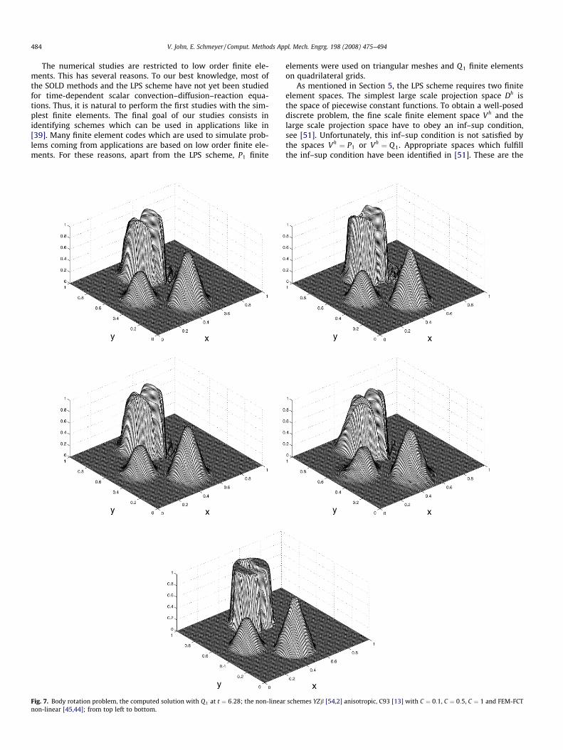
The numerical studies are restricted to low order finite ele-ments. This has several reasons. To our best knowledge, most ofthe SOLD methods and the LPS scheme have not yet been studiedfor time-dependent scalar convection–diffusion–reaction equa-tions. Thus, it is natural to perform the first studies with the sim-plest finite elements. The final goal of our studies consists inidentifying schemes which can be used in applications like in[39]. Many finite element codes which are used to simulate prob-lems coming from applications are based on low order finite ele-ments. For these reasons, apart from the LPS scheme, P1 finite

Fig. 7. Body rotation problem, the computed solution with Q1 at t ¼ 6:28; the non-linearnon-linear [45,44]; from top left to bottom.

elements were used on triangular meshes and Q1 finite elementson quadrilateral grids.

As mentioned in Section 5, the LPS scheme requires two finiteelement spaces. The simplest large scale projection space Dh isthe space of piecewise constant functions. To obtain a well-poseddiscrete problem, the fine scale finite element space Vh and thelarge scale projection space have to obey an inf–sup condition,see [51]. Unfortunately, this inf–sup condition is not satisfied bythe spaces Vh ¼ P1 or Vh ¼ Q 1. Appropriate spaces which fulfillthe inf–sup condition have been identified in [51]. These are the

schemes YZb [54,2] anisotropic, C93 [13] with C ¼ 0:1, C ¼ 0:5, C ¼ 1 and FEM-FCT


spaces Vh=Dh ¼ Pbubble1 =P0 and Vh=Dh ¼ Q bubble

1 =P0, i.e. the standardspaces P1; Q 1 have to be enriched with bubble functions.

In all simulations with SUPG and SOLD schemes, the parameterhK was chosen to be the mesh width of the mesh cell K in the direc-tion of the convection, see the remark at the end of Section 3. Thelength of the mesh cell in the direction of the convection can beeasily approximated, see [55,34]. The SUPG parameters (9)–(11)were scaled with the factor 1.

The non-linear problems for most of the SOLD methods and thenon-linear FEM-FCT method were solved in each discrete time up

Fig. 8. Body rotation problem, the computed solution with P1 (or Pbubble1 =P0 for the LPS sch

with C ¼ 0:01, C ¼ 0:1, C ¼ 1, FEM-FCT linear [43]; from top left to bottom right.

to the Euclidean norm of the residual vector less than 10�9. A sim-ple fixed point iteration was employed, see [36], with a fixeddamping factor. Damping was only applied if the method withoutdamping diverged (a blow-up occurred) or if it did not converge(the non-linear problems could not be solved to the required accu-racy). In applications, it is of advantage if a method works withouta sophisticated choice of the damping factor. We considered damp-ing factors from the set {1,0.75,0.5,0.25}, where we started withthe largest factor. Only if the non-linear iteration did not workfor the given factor, the simulations were repeated with the next

eme) at t ¼ 6:28; the linear schemes SUPG (11) [42,49], JWS87 [41], LPS scheme [50]


smaller damping factor. Smaller damping factors than 0:25 wouldlead to a very large number of iterations to solve the non-linearproblems and thus to inefficient methods. The maximal numberof iterations in each discrete time was set to be 100. The matriceswere assembled in each iteration, which will be also necessary inthe simulation of chemical reactions.

A lot of studies would have been possible with respect to theused meshes and time steps. To keep the paper at a reasonablelength, we restricted the studies to the situation which occurs inthe simulation of precipitation processes [39]: rather small timesteps and grid sizes of medium range. It was checked numerically

Fig. 9. Body rotation problem, the computed solution with P1 at t ¼ 6:28; the non-lineawith C ¼ 1e� 4, BE05_2 [10,34] with C ¼ 1e� 3 and FEM-FCT non-linear [45,44]; from

that the used time steps and grid sizes fulfill the CFL-like condition(30) for the FEM-FCT methods.

All simulations were performed with the code MooNMD [37].The linear systems of equations were solved with the sparse directsolver UMFPACK [17].

7.1. A body rotation problem

The first example is an adaption of the three body rotationtransport problem from [47]. This problem with e ¼ 0 was exten-sively studied in simulations with flux corrected transport finite

r schemes YZb [54,2] anisotropic, KLR02 [42,34] with C ¼ 0:2, C ¼ 0:6, BE05_1 [10]top left to bottom right.

Table 4Hump changing its height, results obtained with P1 (or Pbubble


Method kehkL2ðH1Þ varð0:5Þ Time Damp.

SUPG (9) [15] 13.3334 1.5022 8550 –SUPG (10) [20] 13.3334 1.5022 8535 –SUPG (11) [42,49] 12.1257 1.3835 8550 –


element methods [44,43]. A problem with circular convection wasalso considered in [4].

Consider (1) in X ¼ ð0;1Þ2 with the coefficients e ¼ 10�20, b ¼ð0:5� y; x� 0:5ÞT, c ¼ f ¼ 0. The initial condition consists of threedisjoint bodies, see Fig. 4. The position of each body is given byits center ðx0; y0Þ. Each of the bodies lies within a circle of radiusr0 ¼ 0:15 with the center ðx0; y0Þ. Outside the three bodies, the ini-tial condition is zero.

Let

rðx; yÞ ¼ 1r0

ffiffiffiffiffiffiffiffiffiffiffiffiffiffiffiffiffiffiffiffiffiffiffiffiffiffiffiffiffiffiffiffiffiffiffiffiffiffiffiffiffiffiffiðx� x0Þ2 þ ðy� y0Þ

2q

:

The center of the slotted cylinder is in ðx0; y0Þ ¼ ð0:5;0:75Þ and itsgeometry is given by

uð0; x; yÞ ¼1 if rðx; yÞ 6 1; jx� x0jP 0:0225 or y P 0:85;0 else:

�

The conical body at the bottom side is described by ðx0; y0Þ ¼ð0:5;0:25Þ and

uð0; x; yÞ ¼ 1� rðx; yÞ:

Finally, the hump at the left hand side is given by ðx0; y0Þ ¼ð0:25;0:5Þ and

uð0; x; yÞ ¼ 14ð1þ cosðpminfrðx; yÞ;1gÞÞ:

The rotation of the bodies occurs counter–clockwise. A full revolu-tion takes t ¼ 2p. The original example from [47] is a pure transportproblem, i.e. e ¼ 0, and ideally one should obtain the initial condi-tion after each revolution. But even with the very small diffusione used in our numerical studies, an ideal method should give a re-sult which is very close to the initial condition.

In the simulations, regular grids consisting of 128� 128 trian-gular or rectangular (squared) mesh cells were used. This is thesame grid size which was applied in [44,43]. The number of de-grees of freedom, including Dirichlet nodes, is 16,641. For the LPSscheme, the numbers of degrees of freedom are 33,025/16,384for Q bubble

1 =P0 and 49,409/32,768 for Pbubble1 =P0. In the triangular

Table 3Hump changing its height, results obtained with Q 1 (or Q bubble


Method kehkL2ðH1Þ varð0:5Þ Time Damp.

SUPG (9) [15] 11.2143 1.4282 5297 –SUPG (10) [20] 11.2142 1.4281 5275 –SUPG (11) [42,49] 10.4631 1.3287 5245 –GdC88 [22] 10.4631 1.3287 10,133 1.0dCG91 [19] Not converged 0.25AS97 [1] Not converged 0.25dCA03 [18] 10.4631 1.3287 14,824 1.0YZb [54,2], iso Diverged 0.25YZb [54,2], aniso 9.9861 1.1566 56,944 1.0C93 [13], C ¼ 0:1 10.0980 1.2382 39,826 1.0C93 [13], C ¼ 0:2 9.9485 1.1902 131,413 0.75KLR02 [42,34], C ¼ 0:1 10.0987 1.2381 19,249 1.0KLR02 [42,34], C ¼ 0:2 9.9494 1.1901 22,284 1.0KLR02 [42,34], C ¼ 0:4 9.9334 1.1553 35,022 1.0KLR02 [42,34], C ¼ 0:6 10.1140 1.1347 56,608 1.0KLR02 [42,34], C ¼ 0:8 10.3289 1.1196 83,386 1.0BE02_1 [8] 10.2129 1.2548 16,613 1.0BE02_2 [8,34] 9.9418 1.2027 21,250 1.0JSW87 [41] 9.9255 1.1986 6300 –LPS scheme [50], C ¼ 0:01 30.1938 1.4198 6016 –LPS scheme [50], C ¼ 0:05 14.1264 1.3689 6017 –LPS scheme [50], C ¼ 0:1 11.5793 1.3528 6012 –LPS scheme [50], C ¼ 0:5 10.5392 1.3432 6026 –LPS scheme [50], C ¼ 1 11.2444 1.4474 6013 –LPS scheme [50], C ¼ 5 12.6169 1.5109 6093 –FEM-FCT linear [43] 9.6811 1.0101 2605 –FEM-FCT non-linear [45,44] 9.4399 1.0240 10,051 1.0

grids, the diagonals of the triangles were from bottom left to topright. The simulations were performed with the final timeT ¼ 6:28 and the time step Dt ¼ 10�3. The numerical solutionswere compared with the appropriately rotated initial conditionuðtÞ. Denote the error by eh ¼ u� uh. We present kehkL2ðL2Þ :¼kehkL2ð0;T;L2ðXÞÞ and

varðtÞ :¼ maxðx;yÞ2X

uhðt; x; yÞ � minðx;yÞ2X

uhðt; x; yÞ;

where the maximum and the minimum were computed in the ver-tices of the mesh cells. The values kehkL2ðL2Þ give some indication ofthe accuracy of the methods and the smearing in the numericalsolutions whereas varðtÞ measures the size of the spurious oscilla-tions. The optimal value is varðtÞ ¼ 1 for all t 2 ½0; T�.

First, it is demonstrated that the SUPG method has to be usedwith a parameter including a contribution from the reactive term.A standard parameter for steady-state convection–diffusion equa-tions is

scdK ¼

hK

2kbk2nðPeKÞ; PeK ¼

kbk2hK

2e; nðaÞ ¼ coth a� 1

a: ð31Þ

Fig. 5 shows that the SUPG solution with the parameter (31) is glob-ally polluted with large spurious oscillations whereas the solutionobtained with the parameter (11) possesses large spurious oscilla-tions only at the layers. The spurious oscillations are also consider-ably larger in the solution obtained with scd

K .The results of the computations on the rectangular grid are

summarized in Table 1 and on the triangular grid in Table 2.Among the SUPG methods, the largest parameter (11) gave slightlybetter results than the parameters (9) and (10). All SOLD methodswere used together with the SUPG parameter (11).

GdC88 [22] 12.1257 1.3835 16,331 1.0dCG91 [19] Not converged 0.25AS97 [1] Not converged 0.25dCA03 [18] 12.1257 1.3835 24,513 1.0YZb [54,2], iso Not converged 0.25YZb [54,2], aniso 10.3968 1.1620 153,748 1.0C93 [13], C ¼ 0:1 Diverged 0.25KLR02 [42,34], C ¼ 0:1 10.9608 1.2467 34,462 1.0KLR02 [42,34], C ¼ 0:2 10.5832 1.1970 48,901 1.0KLR02 [42,34], C ¼ 0:4 10.3922 1.1483 84,390 1.0KLR02 [42,34], C ¼ 0:6 10.5113 1.1279 104,510 1.0KLR02 [42,34], C ¼ 0:8 10.7120 1.1179 248,731 0.75BE02_1 [8] 11.5072 1.2985 31,441 1.0BE02_2 [8,34] 10.5888 1.2081 39,154 1.0JSW87 [41] 10.4819 1.1992 10,163 –BH04 [11], C0 ¼ C1 ¼ 1e� 4 Diverged 0.25BE05_1 [10], C ¼ 1e� 5 12.1116 1.3807 16,349 1.0BE05_1 [10], C ¼ 1e� 4 11.9987 1.3558 16,311 1.0BE05_1 [10], C ¼ 1e� 3 11.4126 1.2830 16,222 1.0BE05_1 [10], C ¼ 1e� 2 Diverged 0.25BE05_2 [10,34], C ¼ 1e� 4 12.1168 1.3821 17,379 1.0BE05_2 [10,34], C ¼ 1e� 3 12.0402 1.3695 17,376 1.0BE05_2 [10,34], C ¼ 1e� 2 11.4982 1.2634 17,150 1.0BE05_2 [10,34], C ¼ 1e� 1 10.9352 1.2079 17,109 1.0BE05_2 [10,34], C ¼ 1 Diverged 0.25LPS scheme [50], C ¼ 0:01 68.6146 1.2007 9683 –LPS scheme [50], C ¼ 0:05 19.9672 1.2964 9611 –LPS scheme [50], C ¼ 0:1 15.7470 1.4201 9650 –LPS scheme [50], C ¼ 0:5 19.8025 1.8261 9578 –LPS scheme [50], C ¼ 1 26.2342 1.9659 9614 –LPS scheme [50], C ¼ 2 35.6500 2.1306 9535 –FEM-FCT linear [43] 9.8994 1.0134 3929 –FEM-FCT non-linear [45,44] 9.8254 1.0225 9351 1.0

1

1.1

1.2

1.3

1.4

1.5

1.6

1.7

1.8

1.9

2

var

(t)

SUPG(11)JSW87LPS C = 0.01LPS C = 0.5LPS C = 1FEM−FCT lin.


Remark. Numerical studies (not presented here) showed thatdecreasing the size of the time step, which might be necessary inthe simulation of chemical reactions, gave similar solutions aspresented in Fig. 5 (left picture). Only the size of the spuriousoscillations increased somewhat. These observations are consistentto the analytical results of [4] concerning the stability of the SUPGmethod.

The best results in the body rotation problem were obtainedwith the non-linear FEM-FCT scheme, see Figs. 7 and 9. This isnot surprising since this method was designed for transport prob-lems. Also the linear FEM-FCT method suppressed spurious oscilla-tions but led to some smearing, Figs. 6 and 8.

As expected, the methods GdC88 and dCA03 led to nearly thesame results as the SUPG method. The non-linear iteration didnot converge for the methods dCG91 and AS97. The use of the iso-tropic variant of the YZb scheme resulted in large difficulties in thesolution of the non-linear problems. For the triangular discretiza-tion, this method even blew up for all considered dampingparameters.

The increasing influence of the SOLD term can be observedclearly in the parameter studies for C93 and KLR02. Since D is verysmall in the rotating body problem, these methods gave nearly

0 1 2 3 4 5 6

1

1.1

1.2

1.3

1.4

1.5

1.6

1.7

t

var

(t)

SUPG(11)YZβ, anisoC93 C = 0.1C93 C = 0.5C93 C = 1.0FEM–FCT nonlin.

0 1 2 3 4 5 6

1

1.1

1.2

1.3

1.4

1.5

1.6

1.7

t

var

(t)

SUPG(11)JSW87LPS C = 0.01LPS C = 0.1LPS C = 1LPS C = 5FEM−FCT lin.

Fig. 10. Body rotation problem, evolution of varðtÞ for the solutions computed withQ1 (or Qbubble

1 =P0 for the LPS scheme).

identical results. Large parameters, which make the problemsmore non-linear, led on the one hand to smaller spurious oscilla-tions and larger smearing, see Figs. 7 and 9. On the other hand,some damping in the non-linear iteration became necessary for

0 1 2 3 4 5 6t

0 1 2 3 4 5 6

1

1.1

1.2

1.3

1.4

1.5

1.6

1.7

t

var

(t)

SUPG(11)YZβ, anisoKLR02_3 C = 0.1KLR02_3 C = 0.6BE05_1 C = 1e−4BE05_2 C = 1e−3FEM−FCT nonlin.

Fig. 11. Body rotation problem, evolution of varðtÞ for the solutions computed withP1 (or Pbubble

1 =P0 for the LPS scheme).

0

0.2

0.4

0.6

0.8

1 0

0.2

0.4

0.6

0.8

1

0

0.2

0.4

0.6

0.8

1

yx

Fig. 12. A hump changing its height, solution at t ¼ 0:5.


large parameters, the numbers of iterations to solve the non-linearproblems and accordingly the computing times increased. It is hardto decide which is the best parameter choice if all aspects (spuriousoscillations, smearing, computing times) are taken into consider-ation. The computations on the triangular grid show clearly the dif-ficulties in the solution of the non-linear equations of C93 whicharise from the non-linearity of the second term in (17).

As expected, the SOLD term in BE02_1 and BE02_2 had only lit-tle influence and one obtained similar results as with the SUPGmethod.

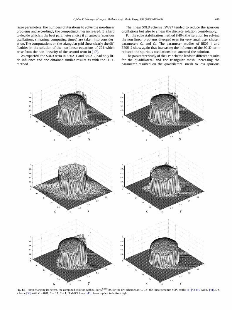
Fig. 13. Hump changing its height, the computed solution with Q1 (or Qbubble1 =P0 for the

scheme [50] with C ¼ 0:01, C ¼ 0:1, C ¼ 1, FEM-FCT linear [43]; from top left to bottom

The linear SOLD scheme JSW87 tended to reduce the spuriousoscillations but also to smear the discrete solution considerably.

For the edge stabilization method BH04, the iteration for solvingthe non-linear problems diverged even for very small user-chosenparameters C0 and C1. The parameter studies of BE05_1 andBE05_2 show again that increasing the influence of the SOLD termreduced the spurious oscillations but smeared the solution.

The parameter study of the LPS scheme leads to different resultsfor the quadrilateral and the triangular mesh. Increasing theparameter resulted on the quadrilateral mesh to less spurious

LPS scheme) at t ¼ 0:5; the linear schemes SUPG with (11) [42,49], JSW87 [41], LPSright.


oscillations and larger smearing, Table 1 and Fig. 6. This situation isvice versa on the triangular mesh, Table 2 and Fig. 8.

The temporal evolution of the spurious oscillations is illustratedin Figs. 10 and 11. For the FEM-FCT schemes, the value varðtÞwas all the time close to the optimal value. Many schemesexhibited rather large spurious oscillations at the beginning ofthe time interval which were smoothed somewhat in later times.Among these schemes are JSW87, C93 and KLR02 for large param-eters, YZb anisotropic and the LPS schemes on the quadrilateralgrid.

7.2. A hump changing its height

This example is an adaption of Example 2 from [38] for the stea-dy-state convection–diffusion–reaction equation. The prescribedsolution has the form

uðt; x; yÞ ¼ 16 sinðptÞxð1� xÞyð1� yÞ

� 12þ arctan½2e�1=2ð0:252 � ðx� 0:5Þ2 � ðy� 0:5Þ2Þ�

p

!:

ð32Þ

This is a hump changing its height in the course of the time, seeFig. 12 for the solution at t ¼ 0:5. The steepness of the circular inter-nal layer depends on the diffusion parameter e. The thickness of thelayer is

ffiffiffiep

which is typical for interior layers [52].

Fig. 14. Hump changing its height, the computed solution with Q1 at t ¼ 0:5; the non-linenon-linear [45,44]; from top left to bottom.

We present simulations for e ¼ 10�6, b ¼ ð2;3Þ, c ¼ 1 and T ¼ 2.In contrast to the previous example, a reactive term of order 1 ap-pears and the right hand side does not vanish. The time step waschosen to be Dt ¼ 10�3 and the computations were performed onthe same grids as in Example 7.1. Hence, the convection is notaligned to the grid.

It is important to note that for the computation of this examplevery accurate quadrature rules, at least for the right hand side, arenecessary. Since the solution possesses a steep layer, the right handside has also regions with large gradients. We found that using loworder quadrature rules leads to a strong pollution of the computedsolutions with all schemes. For the results presented in this sec-tion, Gaussian quadrature which is exact for polynomials of degree17 (81 quadrature points) was used on the quadrilateral mesh. Onthe triangular mesh, a quadrature rule which is exact for polynomi-als of degree 19 (73 quadrature points) was applied. Since in ourcode all matrices and vectors are assembled together, also thematrices have been assembled with the high order quadrature rule.The computing times given below are dominated by the costs ofthe numerical quadrature.

The variation of the discrete solutions at t ¼ 0:5 (maximalheight of the hump) was used for evaluating the size of the spuri-ous oscillations. The value for (32) is varð0:5Þ ¼ 0:997453575. Wealso monitored the variation of the discrete solution at the finaltime T ¼ 2. For almost all schemes, we obtained varð2Þ < 0:04,i.e. rather small oscillations. For this reason, varð2Þ is not reported

ar schemes YZb [54,2] anisotropic, KLR02 [42,34] with C ¼ 0:2, C ¼ 0:6 and FEM-FCT

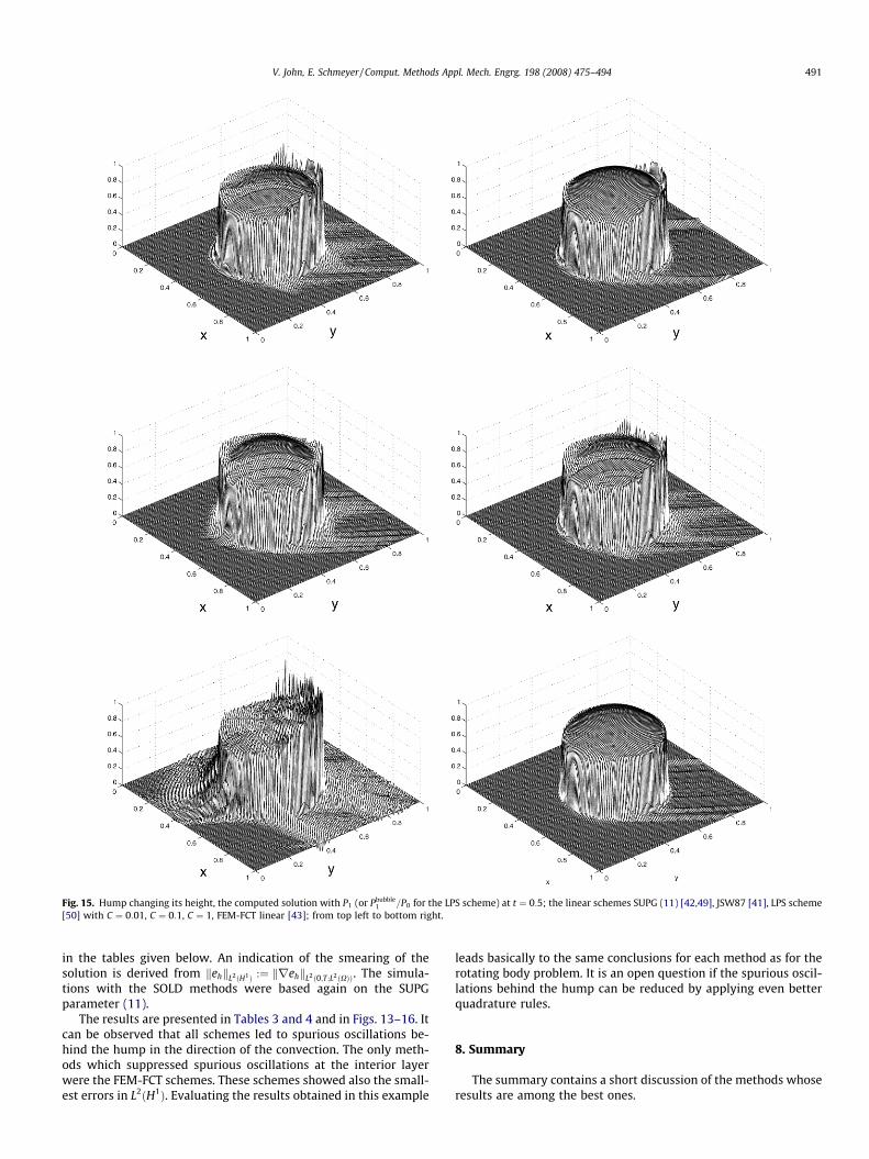
Fig. 15. Hump changing its height, the computed solution with P1 (or Pbubble1 =P0 for the LPS scheme) at t ¼ 0:5; the linear schemes SUPG (11) [42,49], JSW87 [41], LPS scheme

[50] with C ¼ 0:01, C ¼ 0:1, C ¼ 1, FEM-FCT linear [43]; from top left to bottom right.


in the tables given below. An indication of the smearing of thesolution is derived from kehkL2ðH1Þ :¼ krehkL2ð0;T;L2ðXÞÞ. The simula-tions with the SOLD methods were based again on the SUPGparameter (11).

The results are presented in Tables 3 and 4 and in Figs. 13–16. Itcan be observed that all schemes led to spurious oscillations be-hind the hump in the direction of the convection. The only meth-ods which suppressed spurious oscillations at the interior layerwere the FEM-FCT schemes. These schemes showed also the small-est errors in L2ðH1Þ. Evaluating the results obtained in this example

leads basically to the same conclusions for each method as for therotating body problem. It is an open question if the spurious oscil-lations behind the hump can be reduced by applying even betterquadrature rules.

8. Summary

The summary contains a short discussion of the methods whoseresults are among the best ones.

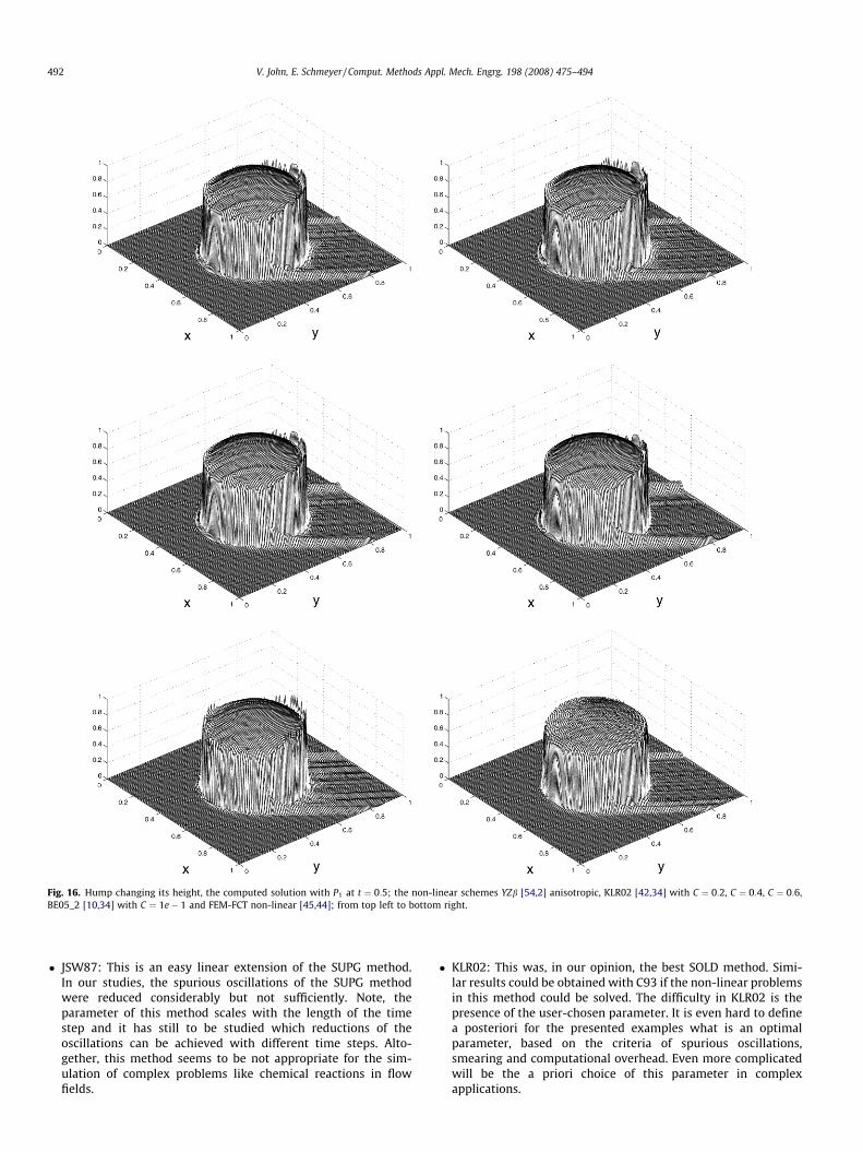
Fig. 16. Hump changing its height, the computed solution with P1 at t ¼ 0:5; the non-linear schemes YZb [54,2] anisotropic, KLR02 [42,34] with C ¼ 0:2, C ¼ 0:4, C ¼ 0:6,BE05_2 [10,34] with C ¼ 1e� 1 and FEM-FCT non-linear [45,44]; from top left to bottom right.


� JSW87: This is an easy linear extension of the SUPG method.In our studies, the spurious oscillations of the SUPG methodwere reduced considerably but not sufficiently. Note, theparameter of this method scales with the length of the timestep and it has still to be studied which reductions of theoscillations can be achieved with different time steps. Alto-gether, this method seems to be not appropriate for the sim-ulation of complex problems like chemical reactions in flowfields.

� KLR02: This was, in our opinion, the best SOLD method. Simi-lar results could be obtained with C93 if the non-linear problemsin this method could be solved. The difficulty in KLR02 is thepresence of the user-chosen parameter. It is even hard to definea posteriori for the presented examples what is an optimalparameter, based on the criteria of spurious oscillations,smearing and computational overhead. Even more complicatedwill be the a priori choice of this parameter in complexapplications.


� YZb aniso: This method gave in the considered examples similarresults to KLR02 with a parameter of C 0:4.

� FEM-FCT schemes: These were clearly the best schemes. InExample 7.2 it is shown that these schemes may lead to somespurious oscillations. In particular, the linear FEM-FCT schemeshows a very good ratio of accuracy and efficiency. The smearingwhich is introduced by this scheme will be tolerable in manyapplications. This scheme has been identified to be a promisingcandidate to be used in the simulation of the chemical reactionsin precipitation processes.

The evaluation of these methods has to be continued. In partic-ular, examples with different boundary conditions than homoge-neous Dirichlet boundary conditions and examples in threedimensions have to be investigated, see [40] for first results. Inaddition, the behavior of the methods with respect to changes inthe length of the time step and the mesh size needs to be studied.

References

[1] R.C. Almeida, R.S. Silva, A stable Petrov–Galerkin method for convection-dominated problems, Comput. Methods Appl. Mech. Engrg. 140 (1997) 291–304.

[2] Y. Bazilevs, V.M. Calo, T.E. Tezduyar, T.J.R. Hughes, YZb discontinuity capturingfor advection-dominated process with applications to arterial drug delivery,Int. J. Numer. Methods Fluids 54 (2007) 593–608.

[3] R. Becker, M. Braack, A finite element pressure gradient stabilization for theStokes equations based on local projections, Calcolo 28 (2001) 173–199.

[4] P.B. Bochev, M.D. Gunzburger, J.N. Shadid, Stability of the SUPG finite elementmethod for transient advection–diffusion problems, Comput. Methods Appl.Mech. Engrg. 193 (2004) 2301–2323.

[5] M. Braack, E. Burman, Local projection stabilization for the Oseen problem andits interpretation as a variational multiscale method, SIAM J. Numer. Anal. 43(2006) 2544–2566.

[6] M. Braack, E. Burman, V. John, G. Lube, Stabilized finite element methods forthe generalized Oseen problem, Comput. Methods Appl. Mech. Engrg. 196(2007) 853–866.

[7] A.N. Brooks, T.J.R. Hughes, Streamline upwind/Petrov–Galerkin formulationsfor convection dominated flows with particular emphasis on theincompressible Navier–Stokes equations, Comput. Methods Appl. Mech.Engrg. 32 (1982) 199–259.

[8] E. Burman, A. Ern, Nonlinear diffusion and discrete maximum principle forstabilized Galerkin approximations of the convection–diffusion–reactionequation, Comput. Methods Appl. Mech. Engrg. 191 (2002) 3833–3855.

[9] E. Burman, A. Ern, The discrete maximum principle for stabilized finite elementmethods, in: F. Brezzi, A. Buffa, S. Corsaro, A. Murli, Numerical mathematicsand advanced applications, Proceedings of the Fourth European Conference(ENUMATH 2001), Springer, Italia, Milan, 2003, pp. 557–566.

[10] E. Burman, A. Ern, Stabilized Galerkin approximation of convection–diffusion–reaction equations: discrete maximum principle and convergence, Math.Comput. 74 (2005) 1637–1652.

[11] E. Burman, P. Hansbo, Edge stabilization for Galerkin approximations ofconvection–diffusion–reaction problems, Comput. Methods Appl. Mech.Engrg. 193 (2004) 1437–1453.

[12] P.G. Ciarlet, The finite element method for elliptic problems, North-HollandPublishing Company, Amsterdam – New York – Oxford, 1978.

[13] R. Codina, A discontinuity-capturing crosswind-dissipation for the finiteelement solution of the convection–diffusion equation, Comput. MethodsAppl. Mech. Engrg. 110 (1993) 325–342.

[14] R. Codina, Comparison of some finite element methods for solving thediffusion–convection–reaction equation, Comput. Methods Appl. Mech.Engrg. 156 (1998) 185–210.

[15] R. Codina, On stabilized finite element methods for linear systems ofconvection–diffusion–reaction equations, Comput. Methods Appl. Mech.Engrg. 188 (2000) 61–82.

[16] R. Codina, J. Blasco, Analysis of stabilized finite element approximation of thetransient convection–diffusion–reaction equation using orthogonal subscales,Comput. Vis. Sci. 4 (2002) 167–174.

[17] T.A. Davis, Algorithm 832: UMFPACK V4.3-an unsymmetric-patternmultifrontal method, ACM Trans. Math. Software 30 (2004) 196–199.

[18] E.G.D. do Carmo, G.B. Alvarez, A new stabilized finite element formulation forscalar convection–diffusion problems: the streamline and approximateupwind/Petrov–Galerkin method, Comput. Methods Appl. Mech. Engrg. 193(2004) 1437–1453.

[19] E.G.D. do Carmo, A.C. Galeão, Feedback Petrov–Galerkin methods forconvection-dominated problems, Comput. Methods Appl. Mech. Engrg. 88(1991) 1–16.

[20] L.P. Franca, F. Valentin, On an improved unusual stabilized finite elementmethod for the advective–reactive–diffusive equation, Comput. Methods Appl.Mech. Engrg. 190 (2000) 1785–1800.

[21] A.C. Galeão, R.C. Almeida, S.M.C. Malta, A.F.D. Loula, Finite element analysis ofconvection dominated reaction–diffusion problems, Appl. Numer. Math. 48(2004) 205–222.

[22] A.C. Galeão, E.G.D. do Carmo, A consistent approximate upwind Petrov–Galerkin method for convection-dominated problems, Comput. Methods Appl.Mech. Engrg. 68 (1988) 83–95.

[23] S. Ganesan, L. Tobiska, Stabilization by local projection. convection–diffusionand incompressible flow problems. Preprint 46, Otto-von-Guericke-Universität Magdeburg, Fakultät für Mathematik, 2007.

[24] V. Gravemeier, W.A. Wall, A space-time formulation and improved spatialreconstruction for the ‘‘divide-and-conquer” multiscale method, Comput.Methods Appl. Mech. Engrg. 197 (2008) 678–692.

[25] J.-L. Guermond, Stabilization of Galerkin approximations of transportequations by subgrid modeling, M2AN 33 (1999) 1293–1316.

[26] G. Hauke, A simple subgrid scale stabilized method for the advection–diffusion–reaction equation, Comput. Methods Appl. Mech. Engrg. 191 (2002)2925–2947.

[27] G. Hauke, M.H. Doweidar, Fourier analysis of semi-discrete and space–timestabilized methods for the advective–diffusive–reactive equation: II. SGS,Comput. Methods Appl. Mech. Engrg. 194 (2005) 691–725.

[28] T.J. Hughes, L. Mazzei, K.E. Jansen, Large eddy simulation and the variationalmultiscale method, Comput. Visual. Sci. 3 (2000) 47–59.

[29] T.J.R. Hughes, Multiscale phenomena: Green’s functions, the Dirichlet-to-Neumann formulation, subgrid-scale models, bubbles and the origin ofstabilized methods, Comput. Methods Appl. Mech. Engrg. 127 (1995) 387–401.

[30] T.J.R. Hughes, A.N. Brooks, A multidimensional upwind scheme with nocrosswind diffusion, in: T.J.R. Hughes (Ed.), Finite Element Methods forConvection Dominated Flows, AMD, vol. 34, ASME, New York, 1979, pp.19–35.

[31] V. John, On large eddy simulation and variational multiscale methods in thenumerical simulation of turbulent incompressible flows, Appl. Math. 51 (2006)321–353.

[32] V. John, S. Kaya, A finite element variational multiscale method for the Navier–Stokes equations, SIAM J. Sci. Comput. 26 (2005) 1485–1503.

[33] V. John, S. Kaya, W. Layton, A two-level variational multiscale method forconvection-dominated convection–diffusion equations, Comput. Meth. Appl.Math. Engrg. 195 (2006) 4594–4603.

[34] V. John, P. Knobloch, A comparison of spurious oscillations at layersdiminishing (sold) methods for convection–diffusion equations: part I – areview, Comput. Methods Appl. Mech. Engrg. 196 (2007) 2197–2215.

[35] V. John, P. Knobloch, On the performance of SOLD methods for convection–diffusion problems with interior layers, Int. J. Comput. Sci. Math. 1 (2007) 245–258.

[36] V. John, P. Knobloch, A comparison of spurious oscillations at layersdiminishing (sold) methods for convection–diffusion equations: part II –analysis for P1 and Q1 finite elements, Comput. Methods Appl. Mech. Engrg.197 (2008) 1997–2014.

[37] V. John, G. Matthies, MooNMD – a program package based on mapped finiteelement methods, Comput. Visual. Sci. 6 (2004) 163–170.

[38] V. John, J.M. Maubach, L. Tobiska, Nonconforming streamline-diffusion-finite-element-methods for convection–diffusion problems, Numer. Math. 78 (1997)165–188.

[39] V. John, M. Roland, T. Mitkova, K. Sundmacher, L. Tobiska, A. Voigt, Simulationsof population balance systems with one internal coordinate using finiteelement methods. Chem. Engrg. Sci., in press.

[40] V. John, E. Schmeyer, On finite element methods for 3d time-dependentconvection–diffusion–reaction equations with small diffusion. Preprint 219,Universität des Saarlandes, Fachrichtung 6.1 – Mathematik, 2008. submittedto the Proceedings of the Conference BAIL 2008, Limerick.

[41] C. Johnson, A.H. Schatz, L.B. Wahlbin, Crosswind smear and pointwise errorsin streamline diffusion finite element methods, Math. Comput. 49 (1987) 25–38.

[42] T. Knopp, G. Lube, G. Rapin, Stabilized finite element methods with shockcapturing for advection–diffusion problems, Comput. Methods Appl. Mech.Engrg. 191 (2002) 2997–3013.

[43] D. Kuzmin, Explicit and implicit FEM-FCT algorithms with flux linearization,Ergebnisberichte Angew. Math. 358, University of Dortmund, 2008.

[44] D. Kuzmin, M. Möller, Algebraic flux correction I. Scalar conservation laws, in:R. Löhner, D. Kuzmin, S. Turek (Eds.), Flux-Corrected Transport: Principles,Algorithms and Applications, Springer, 2005, pp. 155–206.

[45] D. Kuzmin, M. Möller, S. Turek, High-resolution FEM-FCT schemes formultidimensional conservation laws, Comput. Methods Appl. Mech. Engrg.193 (2004) 4915–4946.

[46] D. Kuzmin, S. Turek, Flux correction tools for finite elements, J. Comput. Phys.175 (2002) 525–558.

[47] R.J. LeVeque, High-resolution conservative algorithms for advection inincompressible flow, SIAM J. Numer. Anal. 33 (1996) 627–665.

[48] R. Löhner, K. Morgan, J. Peraire, M. Vahdati, Finite element flux-correctedtransport (FEM-FCT) for the Euler and Navier–Stokes equations, Int. J. Numer.Methods Fluids 7 (1987) 1093–1109.

[49] G. Lube, G. Rapin, Residual-based stabilized higher-order FEM for advection-dominated problems, Comput. Methods Appl. Mech. Engrg. 195 (2006) 4124–4138.

[50] G. Matthies, P. Skrzypacz, L. Tobiska, Stabilisation of local projection typeapplied to convection–diffusion problems with mixed boundary conditions.


Preprint 44, Otto-von-Guericke-Universität Magdeburg, Fakultät fürMathematik, 2007.

[51] G. Matthies, P. Skrzypacz, L. Tobiska, A unified convergence analysis for localprojection stabilisations applied to the Oseen problem, M2AN 41 (2007) 713–742.

[52] H.-G. Roos, M. Stynes, L. Tobiska, Numerical Methods for Singularly PerturbedDifferential Equations, Springer, 1996.

[53] M. Stynes, L. Tobiska, Necessary L2-uniform convergence conditions fordifference schemes for two-dimensional convection–diffusion problems,Comput. Math. Appl. 29 (1995) 45–53.

[54] T.E. Tezduyar, Finite element methods for fluid dynamics with movingboundaries and interfaces, in: E. Stein, R. De Borst, T.J.R. Hughes (Eds.),Encyclopedia of Computational Mechanics, Fluids, vol. 3, Wiley, New York,2004. chapter 17.

[55] T.E. Tezduyar, Y.J. Park, Discontinuity-capturing finite element formulationsfor nonlinear convection–diffusion–reaction equations, Comput. MethodsAppl. Mech. Engrg. 59 (1986) 307–325.

[56] S.T. Zalesak, Fully multi-dimensional flux corrected transport algorithms forfluid flow, J. Comput. Phys. 31 (1979) 335–362.

Date post:	25-May-2018
Category:	Documents
Upload:	trinhduong
View:	218 times
Download:	0 times

Comput. Methods Appl. Mech. Engrg. - Weierstrass … element methods for time-dependent...

Documents