Computation and Application

of

Balanced Model Order Reduction

D.C. Sorensen

I Collaborators: M. Heinkenschloss, A.C. Antoulas and K. Sun

I Support: NSF and AFOSR

MIT Nov 2007

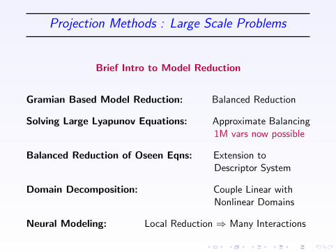
Projection Methods : Large Scale Problems

Brief Intro to Model Reduction

Gramian Based Model Reduction: Balanced Reduction

Solving Large Lyapunov Equations: Approximate Balancing1M vars now possible

Balanced Reduction of Oseen Eqns: Extension toDescriptor System

Domain Decomposition: Couple Linear withNonlinear Domains

Neural Modeling: Local Reduction ⇒ Many Interactions

D.C. Sorensen 2

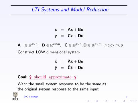
LTI Systems and Model Reduction

x = Ax + Bu

y = Cx + Du

A ∈ Rn×n, B ∈ Rn×m, C ∈ Rp×n,D ∈ Rp×m n >> m, p

Construct LOW dimensional system

˙x = Ax + Bu

y = Cx + Du

Goal: y should approximate y

Want the small system response to be the same asthe original system response to the same input

D.C. Sorensen 3

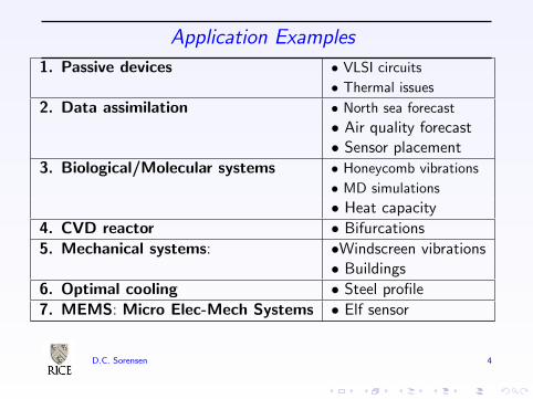
Application Examples

1. Passive devices • VLSI circuits

• Thermal issues

2. Data assimilation • North sea forecast

• Air quality forecast• Sensor placement

3. Biological/Molecular systems • Honeycomb vibrations

• MD simulations

• Heat capacity

4. CVD reactor • Bifurcations

5. Mechanical systems: •Windscreen vibrations• Buildings

6. Optimal cooling • Steel profile

7. MEMS: Micro Elec-Mech Systems • Elf sensor

D.C. Sorensen 4

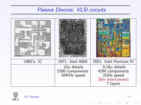
Passive Devices: VLSI circuits

1960’s: IC 1971: Intel 4004 2001: Intel Pentium IV

10µ details 0.18µ details2300 components 42M components

64KHz speed 2GHz speed2km interconnect

7 layers

D.C. Sorensen 5

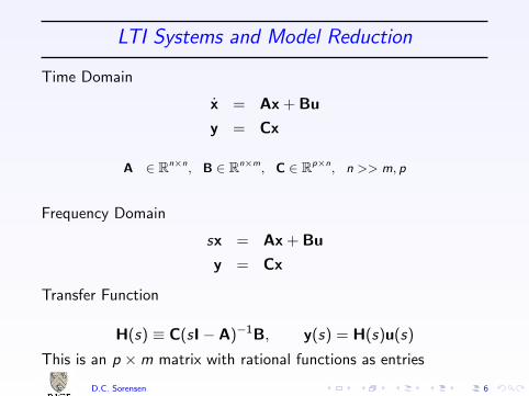
LTI Systems and Model Reduction

Time Domain

x = Ax + Bu

y = Cx

A ∈ Rn×n, B ∈ Rn×m, C ∈ Rp×n, n >> m, p

Frequency Domain

sx = Ax + Bu

y = Cx

Transfer Function

H(s) ≡ C(sI− A)−1B, y(s) = H(s)u(s)

This is an p ×m matrix with rational functions as entries

D.C. Sorensen 6

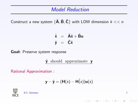
Model Reduction

Construct a new system A, B, C with LOW dimension k << n

˙x = Ax + Bu

y = Cx

Goal: Preserve system response

y should approximate y

Rational Approximation :

y − y = (H(s)− ˆH(s))u(s)

D.C. Sorensen 7

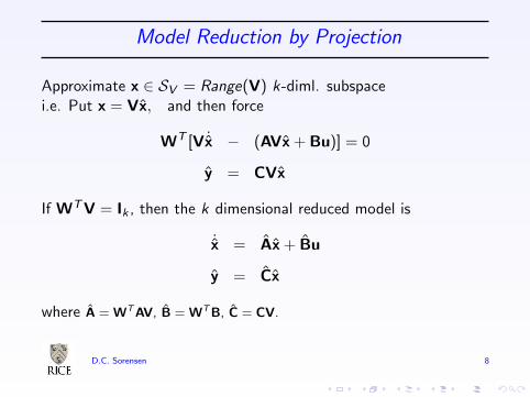
Model Reduction by Projection

Approximate x ∈ SV = Range(V) k-diml. subspacei.e. Put x = Vx, and then force

WT [V ˙x − (AVx + Bu)] = 0

y = CVx

If WTV = Ik , then the k dimensional reduced model is

˙x = Ax + Bu

y = Cx

where A = WTAV, B = WTB, C = CV.

D.C. Sorensen 8

Moment Matching ↔ Krylov Subspace Projection

Based on Lanczos, Arnoldi, Rational Krylov methods

Pade via Lanczos (PVL)

Freund, Feldmann

Bai

Multipoint Rational Interpolation

Grimme

Gallivan, Grimme, Van Dooren

Recent: Optimal H2 approximation via interpolationGugercin, Antoulas, Beattie

D.C. Sorensen 9

Gramian Based Model Reduction

Proper Orthogonal Decomposition (POD)Principal Component Analysis (PCA)

x(t) = f(x(t),u(t)), y = g(x(t),u(t))

The Gramian

P =

∫ ∞

ox(τ)x(τ)Tdτ

Eigenvectors of P

P = VS2VT

Orthogonal Basisx(t) = VSw(t)

D.C. Sorensen 10

PCA or POD Reduced Basis

Low Rank Approximation

x ≈ Vk xk(t)

Galerkin condition – Global Basis

˙xk = VTk f(Vk xk(t),u(t))

Global Approximation Error (H2 bound for LTI)

‖x− Vk xk‖2 ≈ σk+1

Snapshot Approximation to P

P ≈ 1

m

m∑j=1

x(tj)x(tj)T = XXT

Truncate SVD : X = VSUT ≈ VkSkUTk

SVD Compression

m

k ( m + n)

m x n

v.s.

Storage

Advantage of SVD Compression

k

n

0 20 40 60 80 100 120 140 160 180 2000

10

20

30

40

50

60

70

80

90

100SVD of Clown

D.C. Sorensen 12

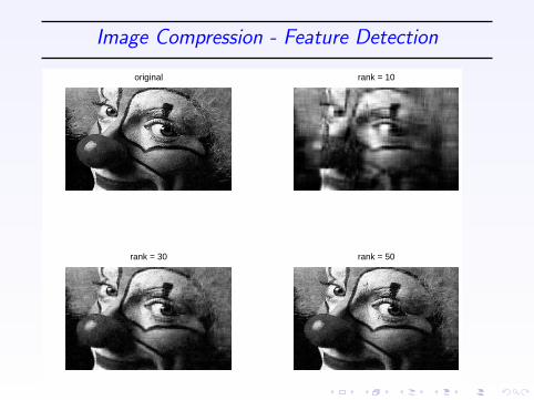
Image Compression - Feature Detection

original rank = 10

rank = 30 rank = 50

POD in CFD

Extensive Literature

Karhunen-Loeve, L. Sirovich

Burns, King

Kunisch and Volkwein

Gunzburger

Many, many others

Incorporating Observations – Balancing

Lall, Marsden and Glavaski

K. Willcox and J. Peraire

D.C. Sorensen 14

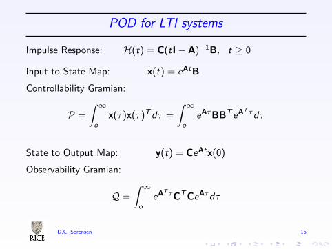
POD for LTI systems

Impulse Response: H(t) = C(tI− A)−1B, t ≥ 0

Input to State Map: x(t) = eAtB

Controllability Gramian:

P =

∫ ∞

ox(τ)x(τ)Tdτ =

∫ ∞

oeAτBBT eAT τdτ

State to Output Map: y(t) = CeAtx(0)

Observability Gramian:

Q =

∫ ∞

oeAT τCTCeAτdτ

D.C. Sorensen 15

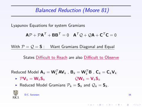
Balanced Reduction (Moore 81)

Lyapunov Equations for system Gramians

AP + PAT + BBT = 0 ATQ+QA + CTC = 0

With P = Q = S : Want Gramians Diagonal and Equal

States Difficult to Reach are also Difficult to Observe

Reduced Model Ak = WTk AVk , Bk = WT

k B , Ck = CkVk

I PVk = WkSk QWk = VkSk

I Reduced Model Gramians Pk = Sk and Qk = Sk .

D.C. Sorensen 16

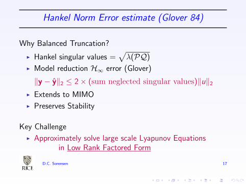
Hankel Norm Error estimate (Glover 84)

Why Balanced Truncation?

I Hankel singular values =√

λ(PQ)

I Model reduction H∞ error (Glover)

‖y − y‖2 ≤ 2× (sum neglected singular values)‖u‖2I Extends to MIMO

I Preserves Stability

Key Challenge

I Approximately solve large scale Lyapunov Equationsin Low Rank Factored Form

D.C. Sorensen 17

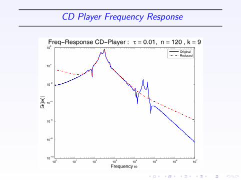
CD Player Frequency Response

100

101

102

103

104

105

106

107

10−10

10−8

10−6

10−4

10−2

100

102

Freq−Response CD−Player : τ = 0.01, n = 120 , k = 9|G

(jω)|

Frequency ω

OriginalReduced

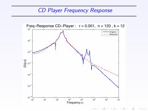
CD Player Frequency Response

100

101

102

103

104

105

106

107

10−10

10−8

10−6

10−4

10−2

100

102

Freq−Response CD−Player : τ = 0.001, n = 120 , k = 12|G

(jω)|

Frequency ω

OriginalReduced

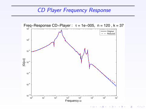
CD Player Frequency Response

100

101

102

103

104

105

106

107

10−10

10−8

10−6

10−4

10−2

100

102

Freq−Response CD−Player : τ = 1e−005, n = 120 , k = 37|G

(jω)|

Frequency ω

OriginalReduced

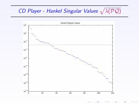
CD Player - Hankel Singular Values√

λ(PQ)

0 20 40 60 80 100 12010

−14

10−12

10−10

10−8

10−6

10−4

10−2

100

102

Hankel Singular Values

D.C. Sorensen 21

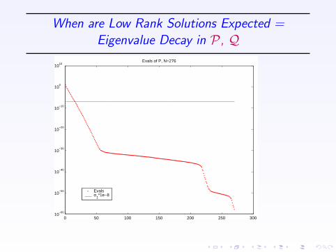
When are Low Rank Solutions Expected =Eigenvalue Decay in P , Q

0 50 100 150 200 250 30010

−60

10−50

10−40

10−30

10−20

10−10

100

1010

Evals of P, N=276

Evalsσ

1*1e−8

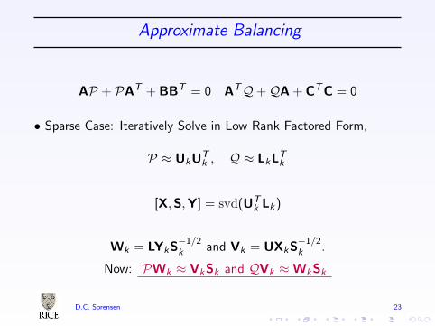
Approximate Balancing

AP + PAT + BBT = 0 ATQ+QA + CTC = 0

• Sparse Case: Iteratively Solve in Low Rank Factored Form,

P ≈ UkUTk , Q ≈ LkL

Tk

[X,S,Y] = svd(UTk Lk)

Wk = LYkS−1/2k and Vk = UXkS

−1/2k .

Now: PWk ≈ VkSk and QVk ≈WkSk

D.C. Sorensen 23

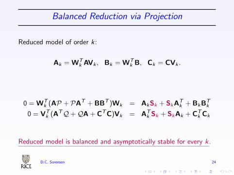
Balanced Reduction via Projection

Reduced model of order k:

Ak = WTk AVk , Bk = WT

k B, Ck = CVk .

0 = WTk (AP + PAT + BBT )Wk = AkSk + SkA

Tk + BkB

Tk

0 = VTk (ATQ+QA + CTC)Vk = AT

k Sk + SkAk + CTk Ck

Reduced model is balanced and asymptotically stable for every k.

D.C. Sorensen 24

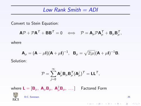
Low Rank Smith = ADI

Convert to Stein Equation:

AP + PAT + BBT = 0 ⇐⇒ P = AµPATµ + BµB

Tµ ,

where

Aµ = (A− µI)(A + µI)−1, Bµ =√

2|µ|(A + µI)−1B.

Solution:

P =∞∑j=0

AjµBµB

Tµ (Aj

µ)T = LLT ,

where L = [Bµ, AµBµ, A2µBµ, . . . ] Factored Form

D.C. Sorensen 25

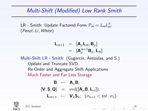
Multi-Shift (Modified) Low Rank Smith

LR - Smith: Update Factored Form Pm = LmLTm:

(Penzl , Li ,White)

Lm+1 = [AµLm,Bµ]

= [Am+1µ Bµ,Lm]

Multi-Shift LR - Smith: (Gugercin, Antoulas, and S.)Update and Truncate SVDRe-Order and Aggregate Shift ApplicationsMuch Faster and Far Less Storage

B ← AµB;

[V,S,Q] = svd([AµB,Lm]);

Lm+1 ← VkSk ; (σk+1 < tol · σ1)

D.C. Sorensen 26

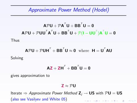
Approximate Power Method (Hodel)

APU + PATU + BB

TU = 0

APU + PUUTA

TU + BB

TU + P(I−UU

T)A

TU = 0

Thus

APU + PUHT

+ BBTU ≈ 0 where H = U

TAU

Solving

AZ + ZHT

+ BBTU = 0

gives approximation to

Z ≈ PU

Iterate ⇒ Approximate Power Method Zj → US with PU = US

(also see Vasilyev and White 05)

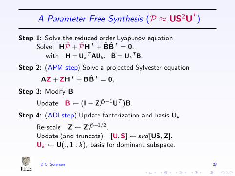
A Parameter Free Synthesis (P ≈ US2UT

)

Step 1: Solve the reduced order Lyapunov equationSolve HP + PHT + BBT = 0.

with H = UkTAUk , B = Uk

TB.

Step 2: (APM step) Solve a projected Sylvester equation

AZ + ZHT + BBT = 0,

Step 3: Modify B

Update B← (I− ZP−1UT )B.

Step 4: (ADI step) Update factorization and basis Uk

Re-scale Z← ZP−1/2.Update (and truncate) [U,S]← svd [US,Z].Uk ← U(:, 1 : k), basis for dominant subspace.

D.C. Sorensen 28

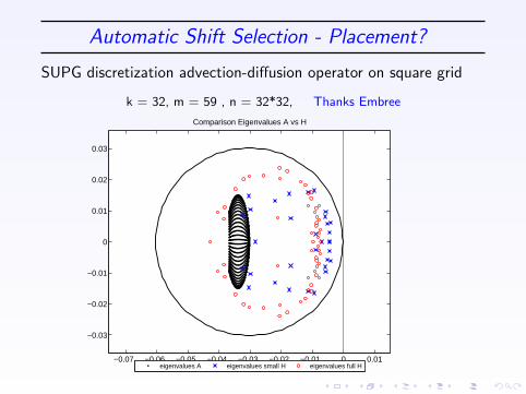
Automatic Shift Selection - Placement?

SUPG discretization advection-diffusion operator on square grid

k = 32, m = 59 , n = 32*32, Thanks Embree

−0.07 −0.06 −0.05 −0.04 −0.03 −0.02 −0.01 0 0.01

−0.03

−0.02

−0.01

0

0.01

0.02

0.03

Comparison Eigenvalues A vs H

eigenvalues A eigenvalues small H eigenvalues full H

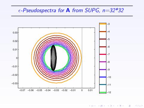
ε-Pseudospectra for A from SUPG, n=32*32

−0.07 −0.06 −0.05 −0.04 −0.03 −0.02 −0.01 0 0.01

−0.03

−0.02

−0.01

0

0.01

0.02

0.03

−12

−11

−10

−9

−8

−7

−6

−5

−4

−3

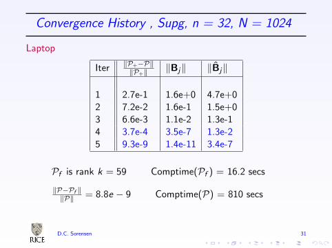
Convergence History , Supg, n = 32, N = 1024

Laptop

Iter ‖P+−P‖‖P+‖ ‖Bj‖ ‖Bj‖

1 2.7e-1 1.6e+0 4.7e+02 7.2e-2 1.6e-1 1.5e+03 6.6e-3 1.1e-2 1.3e-14 3.7e-4 3.5e-7 1.3e-25 9.3e-9 1.4e-11 3.4e-7

Pf is rank k = 59 Comptime(Pf ) = 16.2 secs

‖P−Pf ‖‖P‖ = 8.8e − 9 Comptime(P) = 810 secs

D.C. Sorensen 31

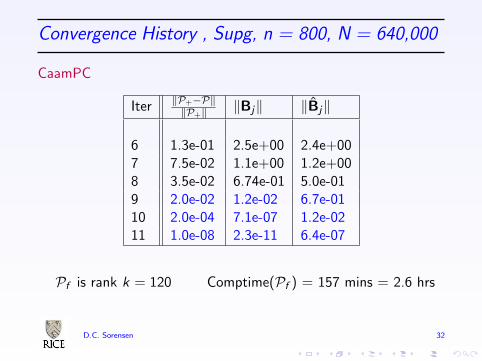
Convergence History , Supg, n = 800, N = 640,000

CaamPC

Iter ‖P+−P‖‖P+‖ ‖Bj‖ ‖Bj‖

6 1.3e-01 2.5e+00 2.4e+007 7.5e-02 1.1e+00 1.2e+008 3.5e-02 6.74e-01 5.0e-019 2.0e-02 1.2e-02 6.7e-0110 2.0e-04 7.1e-07 1.2e-0211 1.0e-08 2.3e-11 6.4e-07

Pf is rank k = 120 Comptime(Pf ) = 157 mins = 2.6 hrs

D.C. Sorensen 32

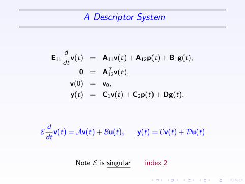
A Descriptor System

E11d

dtv(t) = A11v(t) + A12p(t) + B1g(t),

0 = AT12v(t),

v(0) = v0,

y(t) = C1v(t) + C2p(t) + Dg(t).

E d

dtv(t) = Av(t) + Bu(t), y(t) = Cv(t) +Du(t)

Note E is singular index 2

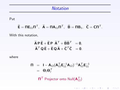
Notation

Put

E = ΠE11ΠT , A = ΠA11Π

T , B = ΠB1, C = CΠT .

With this notation,

A P E + E P AT + BBT = 0,

AT QE + EQ A + CT C = 0.

where

Π = I− A12(AT12E

−111 A12)

−1AT12E

−111

= ΘlΘTr

ΠT Projector onto Null(AT12)

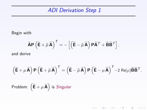
ADI Derivation Step 1

Begin with

AP(E + µ A

)T= −

[(E− µ A

)PAT + BBT

].

and derive

(E + µ A

)P

(E + µ A

)T=

(E− µ A

)P

(E− µ A

)T−2 Re(µ)BBT .

Problem:(E + µ A

)is Singular

Key Pseudo-Inverse Lemma

Suppose ΘTr E11Θr + µΘT

r A11Θr is invertible.

Then the matrix(E + µ A

)I≡ Θr

(ΘT

r E11Θr + µΘTr A11Θr

)−1ΘT

r

satisfies (E + µ A

)I (E + µ A

)= ΠT

and (E + µ A

) (E + µ A

)I= Π.

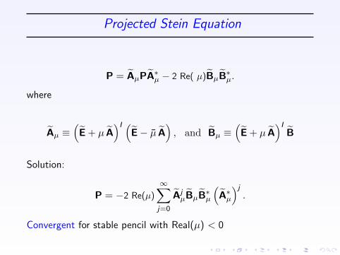
Projected Stein Equation

P = AµPA∗µ − 2 Re( µ)BµB

∗µ.

where

Aµ ≡(E + µ A

)I (E− µ A

), and Bµ ≡

(E + µ A

)IB

Solution:

P = −2 Re(µ)

∞∑j=0

AjµBµB

∗µ

(A∗

µ

)j.

Convergent for stable pencil with Real(µ) < 0

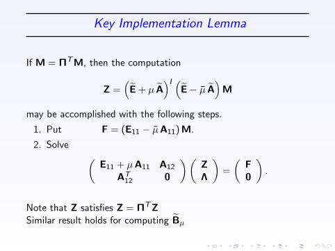
Key Implementation Lemma

If M = ΠTM, then the computation

Z =(E + µ A

)I (E− µ A

)M

may be accomplished with the following steps.

1. Put F = (E11 − µA11)M.

2. Solve (E11 + µA11 A12

AT12 0

) (ZΛ

)=

(F0

).

Note that Z satisfies Z = ΠTZSimilar result holds for computing Bµ

Algorithm:Single Shift ADI

1. Solve

(E11 + µA11 A12

AT12 0

) (ZΛ

)=

(B0

);

2. U = Z;

3. while ( ’not converged’)

3.1 Z← (E11 − µA11)Z;

3.2 Solve (in place)

(E11 + µA11 A12

AT12 0

) (ZΛ

)=

(Z0

);

3.3 U← [U,Z] ;

end

4. U←√

2| Re(µ)|U.

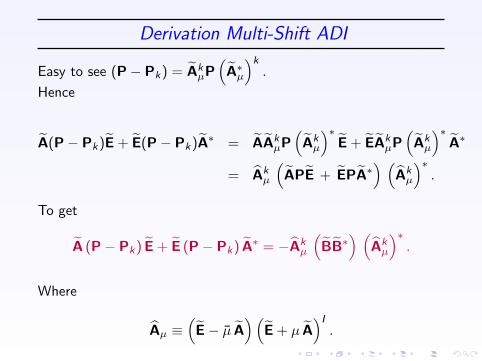
Derivation Multi-Shift ADI

Easy to see (P− Pk) = AkµP

(A∗

µ

)k.

Hence

A(P− Pk)E + E(P− Pk)A∗ = AAkµP

(Ak

µ

)∗E + EAk

µP(Ak

µ

)∗A∗

= Akµ

(APE + EPA∗

) (Ak

µ

)∗.

To get

A (P− Pk) E + E (P− Pk) A∗ = −Akµ

(BB∗

) (Ak

µ

)∗.

Where

Aµ ≡(E− µ A

) (E + µ A

)I.

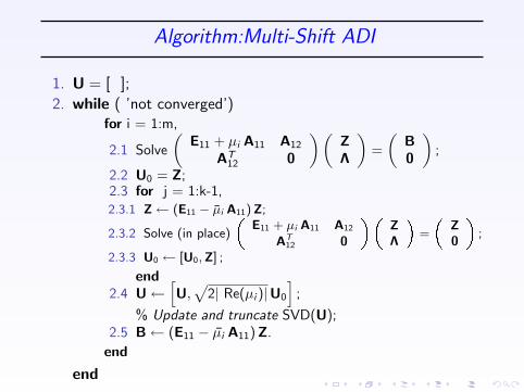
Algorithm:Multi-Shift ADI

1. U = [ ];

2. while ( ’not converged’)for i = 1:m,

2.1 Solve

(E11 + µi A11 A12

AT12 0

) (ZΛ

)=

(B0

);

2.2 U0 = Z;2.3 for j = 1:k-1,2.3.1 Z← (E11 − µi A11)Z;

2.3.2 Solve (in place)

E11 + µi A11 A12

AT12 0

ZΛ

=

Z0

;

2.3.3 U0 ← [U0,Z] ;

end2.4 U←

[U,

√2| Re(µi )|U0

];

% Update and truncate SVD(U);2.5 B← (E11 − µi A11)Z.

end

end

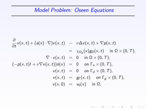
Model Problem: Oseen Equations

∂

∂tv(x , t) + (a(x) · ∇)v(x , t) − ν∆v(x , t) +∇p(x , t)

= χΩg (x)gΩ(x , t) in Ω× (0,T ),

∇ · v(x , t) = 0 in Ω× (0,T ),

(−p(x , t)I + ν∇v(x , t))n(x) = 0 on Γn × (0,T ),

v(x , t) = 0 on Γd × (0,T ),

v(x , t) = gΓ(x , t) on Γg × (0,T ),

v(x , 0) = v0(x) in Ω,

Channel Geometry and Grid

0 1 2 3 4 5 6 7 80

0.5

1

Figure: The channel geometry and coarse grid

EXAMPLE 1.

y(t) =

∫Ωobs

−∂x2v1(x , t) + ∂x1v2(x , t)dx

over the subdomain Ωobs = (1, 3)× (0, 1/2).

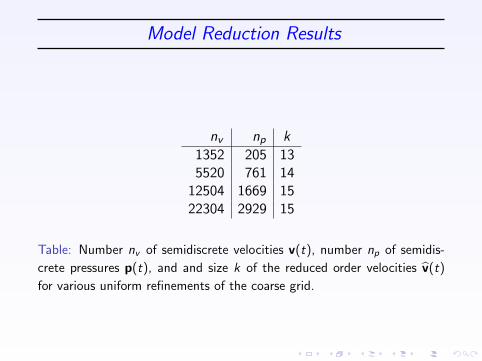
Model Reduction Results

nv np k

1352 205 135520 761 14

12504 1669 1522304 2929 15

Table: Number nv of semidiscrete velocities v(t), number np of semidis-

crete pressures p(t), and and size k of the reduced order velocities v(t)

for various uniform refinements of the coarse grid.

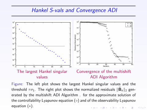
Hankel S-vals and Convergence ADI

0 5 10 15 20 25 3010

−7

10−6

10−5

10−4

10−3

10−2

10−1

100

101

The largest Hankel singularvalues

0 10 20 30 40 50 6010

−7

10−6

10−5

10−4

10−3

10−2

10−1

100

Iteration

Res

idua

l (N

orm

aliz

ed)

PQ

Convergence of the multishiftADI Algorithm

Figure: The left plot shows the largest Hankel singular values and the

threshold τσ1. The right plot shows the normalized residuals ‖Bk‖2 gen-

erated by the multishift ADI Algorithm . for the approximate solution of

the controllability Lyapunov equation () and of the observability Lyapunov

equation (∗).

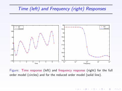
Time (left) and Frequency (right) Responses

0 1 2 3 4 5 6 7−150

−100

−50

0

50

100

150

Time

fullreduced

10−4

10−2

100

102

104

75.5

76

76.5

77

77.5

78

78.5

79

79.5

80

Frequency

fullreduced

Figure: Time response (left) and frequency response (right) for the full

order model (circles) and for the reduced order model (solid line).

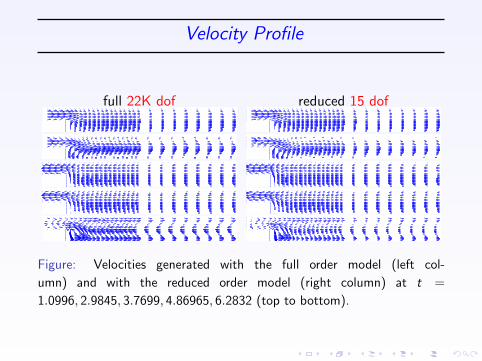
Velocity Profile

full 22K dof reduced 15 dof

Figure: Velocities generated with the full order model (left col-

umn) and with the reduced order model (right column) at t =

1.0996, 2.9845, 3.7699, 4.86965, 6.2832 (top to bottom).

Domain Decomposition Model Reduction

Systems with Local Nonlinearities

Linear Model in Large Domain Ω1

coupled to

Non-Linear Model in Small Domain Ω2

Linear Model provides B.C.’s to Non-Linear Model

with R. Glowinski

D.C. Sorensen 48

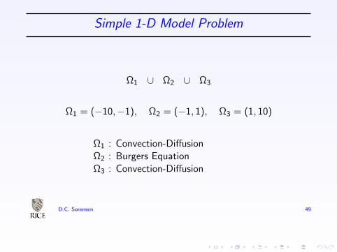
Simple 1-D Model Problem

Ω1 ∪ Ω2 ∪ Ω3

Ω1 = (−10,−1), Ω2 = (−1, 1), Ω3 = (1, 10)

Ω1 : Convection-DiffusionΩ2 : Burgers EquationΩ3 : Convection-Diffusion

D.C. Sorensen 49

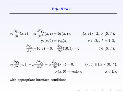
Equations

ρk∂yk

∂t(x , t)− µk

∂2yk

∂x2(x , t) = Sk(x , t), (x , t) ∈ Ωk × (0,T ),

yk(x , 0) = yk0(x), x ∈ Ωk , k = 1, 3,

∂y1

∂x(−10, t) = 0,

∂y3

∂x(10, t) = 0 t ∈ (0,T ),

ρ2∂y2

∂t(x , t)− µ2

∂2y2

∂x2+ y2

∂y2

∂x(x , t) = 0, (x , t) ∈ Ω2 × (0,T ),

y2(x , 0) = y20(x), x ∈ Ω2,

with appropriate interface conditions

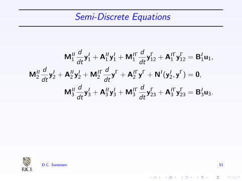
Semi-Discrete Equations

MII1

d

dtyI1 + AII

1 yI1 + MIΓ

1

d

dtyΓ12 + AIΓ

1 yΓ12 = BI

1u1,

MII2

d

dtyI2 + AII

2 yI2 + MIΓ

2

d

dtyΓ + AIΓ

2 yΓ + NI (yI2, y

Γ) = 0,

MII3

d

dtyI3 + AII

3 yI3 + MIΓ

3

d

dtyΓ23 + AIΓ

3 yΓ23 = BI

3u3.

D.C. Sorensen 51

Equations to Reduce

Inputs to System 1: MIΓ1

ddt y

Γ12, AIΓ

1 yΓ12 and BI

1u1

Outputs of System 1: CΓI1 yI

1, MΓI1

ddt y

I1 + AΓI

1 yI1

Apply Model Reduction to

MII1

d

dtyI1 = −AII

1 yI1 − AIΓ

1 yΓ12 + BI

1u1

zI1 = CI

1yI1, zΓ

1 = AΓI1 yI

1.

D.C. Sorensen 52

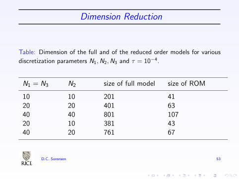
Dimension Reduction

Table: Dimension of the full and of the reduced order models for various

discretization parameters N1,N2,N3 and τ = 10−4.

N1 = N3 N2 size of full model size of ROM

10 10 201 4120 20 401 6340 40 801 10720 10 381 4340 20 761 67

D.C. Sorensen 53

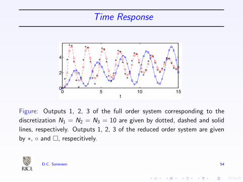
Time Response

0 5 10 150

2

4

t

Figure: Outputs 1, 2, 3 of the full order system corresponding to the

discretization N1 = N2 = N3 = 10 are given by dotted, dashed and solid

lines, respectively. Outputs 1, 2, 3 of the reduced order system are given

by ∗, and , respecitively.

D.C. Sorensen 54

State Approximation

!10 !5 0 5 10

0

5

10

15!5

0

5

10

x

t!10 !5 0 5 10

0

5

10

15!0.02

0

0.02

0.04

x

t

Figure: Solution of the reduced order discretized PDE (left) and error

between the solution of the discretized PDE and the reduced order system

(right) for discretization N1 = N2 = N3 = 10.

D.C. Sorensen 55

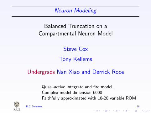
Neuron Modeling

Balanced Truncation on aCompartmental Neuron Model

Steve Cox

Tony Kellems

Undergrads Nan Xiao and Derrick Roos

Quasi-active integrate and fire model.Complex model dimension 6000Faithfully approximated with 10-20 variable ROM

D.C. Sorensen 56

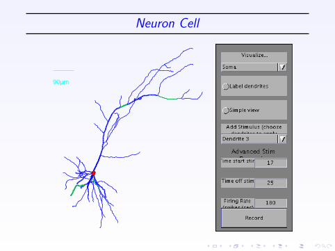
Neuron Cell

90µm

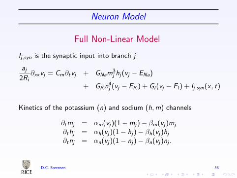
Neuron Model

Full Non-Linear Model

Ij ,syn is the synaptic input into branch j

aj

2Ri∂xxvj = Cm∂tvj + GNam

3j hj(vj − ENa)

+ GKn4j (vj − EK ) + Gl(vj − El) + Ij ,syn(x , t)

Kinetics of the potassium (n) and sodium (h,m) channels

∂tmj = αm(vj)(1−mj)− βm(vj)mj

∂thj = αh(vj)(1− hj)− βh(vj)hj

∂tnj = αn(vj)(1− nj)− βn(vj)nj .

D.C. Sorensen 58

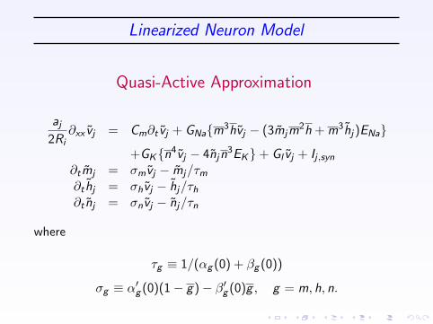
Linearized Neuron Model

Quasi-Active Approximation

aj

2Ri∂xx vj = Cm∂t vj + GNam3hvj − (3mjm

2h + m3hj)ENa

+GKn4vj − 4njn3EK+ Gl vj + Ij ,syn

∂tmj = σmvj − mj/τm

∂t hj = σhvj − hj/τh

∂t nj = σnvj − nj/τn

where

τg ≡ 1/(αg (0) + βg (0))

σg ≡ α′g (0)(1− g)− β′g (0)g , g = m, h, n.

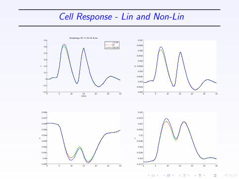
Cell Response - Lin and Non-Lin

0 5 10 15 20 25 30−0.2

−0.1

0

0.1

0.2

0.3

0.4

0.5

0.6v

Morphology: RC−3−04−04−B.asc

t (ms)

0 5 10 15 20 25 300.052

0.0525

0.053

0.0535

0.054

0.0545

0.055

0.0555

0.056

0.0565

0.057

m

0 5 10 15 20 25 300.589

0.59

0.591

0.592

0.593

0.594

0.595

0.596

0.597

0.598

h

0 5 10 15 20 25 300.3175

0.318

0.3185

0.319

0.3195

0.32

0.3205

0.321

0.3215

0.322

n

Lin HHBTFull HH

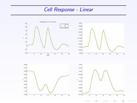
Cell Response - Linear

0 5 10 15 20 25 30−0.2

−0.1

0

0.1

0.2

0.3

0.4

0.5

0.6v

Morphology: RC−3−04−04−B.asc

t (ms)

0 5 10 15 20 25 300.052

0.0525

0.053

0.0535

0.054

0.0545

0.055

0.0555

0.056

0.0565

0.057

m

0 5 10 15 20 25 300.589

0.59

0.591

0.592

0.593

0.594

0.595

0.596

0.597

0.598

h

0 5 10 15 20 25 300.3175

0.318

0.3185

0.319

0.3195

0.32

0.3205

0.321

0.3215

0.322

n

Lin HHBTFull HH

Cell Response - Near Threshold

0 5 10 15 20 25 30−1

−0.5

0

0.5

1

1.5

2v

Morphology: RC−3−04−04−B.asc

t (ms)

0 5 10 15 20 25 300.045

0.05

0.055

0.06

0.065

0.07

m

0 5 10 15 20 25 30

0.565

0.57

0.575

0.58

0.585

0.59

0.595

0.6

0.605

h

0 5 10 15 20 25 300.315

0.32

0.325

0.33

0.335

0.34

n

Lin HHBTFull HH

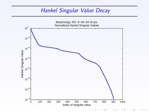
Hankel Singular Value Decay

0 100 200 300 400 500 600 700 800 900 100010

−70

10−60

10−50

10−40

10−30

10−20

10−10

100

Index of singular value

Han

kel S

ingu

lar

Val

ueMorphology: RC−3−04−04−B.asc

Normalized Hankel Singular Values

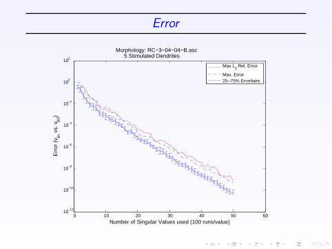
Error

0 10 20 30 40 50 6010−12

10−10

10−8

10−6

10−4

10−2

100

102

Number of Singular Values used (100 runs/value)

Err

or (

v lin v

s. v

BT)

Morphology: RC−3−04−04−B.asc 5 Stimulated Dendrites

Max L

2 Rel. Error

Max. Error25−75% Errorbars

Neural ROM Results

I Interesting example of many-input , single-output system

I Simulation time single cell 14 sec Full vs .01 sec Reduced

I Ultimate goal is to simulate a few-Million neuron systemover a minute of brain-time

I Currently limited to a 10K neuron systemover a few brain-seconds

I Parallel computing required

D.C. Sorensen 65

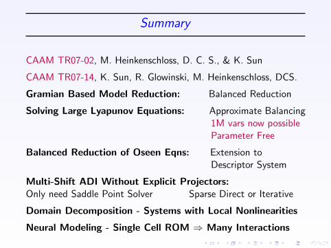
Summary

CAAM TR07-02, M. Heinkenschloss, D. C. S., & K. Sun

CAAM TR07-14, K. Sun, R. Glowinski, M. Heinkenschloss, DCS.

Gramian Based Model Reduction: Balanced Reduction

Solving Large Lyapunov Equations: Approximate Balancing1M vars now possibleParameter Free

Balanced Reduction of Oseen Eqns: Extension toDescriptor System

Multi-Shift ADI Without Explicit Projectors:Only need Saddle Point Solver Sparse Direct or Iterative

Domain Decomposition - Systems with Local Nonlinearities

Neural Modeling - Single Cell ROM ⇒ Many Interactions