111 CHAPTER 4 COMPUTATION OF AVAILABLE TRANSFER CAPABILITY 4.1 INTRODUCTION As discussed in the previous chapters, load flow study plays a vital role in operation and control of modern power systems. It can also be used for the computation of transfer capability. In a deregulated system, the information about the transfer capability will help the energy marketers in reserving the transmission services. For secured and economic supply of electric power, long distance bulk power transfers are essential, but the power transfer capability of a power system is limited. To operate the power systems safely and to gain the advantages of bulk power transfers, computations of transfer capability is essential. Transfer capability plays a vital role in liberalized electricity market. All the transmission lines are utilized significantly below their physical limits due to various constraints. By increasing the transfer capability the economic value of transmission lines can be improved and also there will be an increase in overall efficiency as more energy trading can take place between the competing regions operating with different price structures. The power system should be planned and operated such that these power transfers are within the limits of the system transfer capability.
Transcript
111
CHAPTER 4
COMPUTATION OF AVAILABLE TRANSFER
CAPABILITY
4.1 INTRODUCTION
As discussed in the previous chapters, load flow study plays a vital
role in operation and control of modern power systems. It can also be
used for the computation of transfer capability. In a deregulated system,
the information about the transfer capability will help the energy
marketers in reserving the transmission services. For secured and
economic supply of electric power, long distance bulk power transfers are
essential, but the power transfer capability of a power system is limited.
To operate the power systems safely and to gain the advantages of bulk
power transfers, computations of transfer capability is essential. Transfer
capability plays a vital role in liberalized electricity market. All the
transmission lines are utilized significantly below their physical limits
due to various constraints. By increasing the transfer capability the
economic value of transmission lines can be improved and also there will
be an increase in overall efficiency as more energy trading can take place
between the competing regions operating with different price structures.
The power system should be planned and operated such that these
power transfers are within the limits of the system transfer capability.
112
Transfer capability of a power system is defined as the maximum power
that can be transferred from one area to another area.
4.2 GENERAL MOTIVATION
In open access transmission system, the transmission network
owners are required to provide unbundled services to support power
transactions and to maintain reliable operation of the networks. In a
liberalized electricity markets, to enforce the open access policy North
American Energy Reliability Council (NERC) in conjunction with Federal
Energy Regulatory Commission (FERC) defined the term available
transfer capability (ATC) to be posted in open access same time
information system (OASIS) to inform all the energy market participants
of a power system. This information is required to be made available on
hourly or daily basis. The two major challenges that make the task of
ATC calculation of a nonlinear power system more challenging are
computing speed and accuracy due to static and dynamic security
constraints.
Deregulation of power market has imposed great impact on the
utility industry. For smooth transaction of power between the areas or
paths new technologies and computation methods are urgently needed.
Transfer capability of a power system also indicates how much inter area
power transfer can be increased without system security violations. The
vital information required for the planning and operation of the large
power systems can be obtained from these transfer capability
113
calculations. These details provide system bottlenecks to the planners
and the limits of the power transfers to the system operators. The risk of
overloads, equipment damage and unexpected blackouts can be reduced
by repeated estimation of these transfer capabilities. These calculations
also help to determine the quantity of lost generation that can be
replaced by potential reserves and limiting constraints in each
circumstance.
Due to the deregulation of power systems the power transfers are
increasing which is necessary for a competitive market for electric power.
There is a strong economic incentive to improve the accuracy and
effectiveness of the transfer capability computations for the use by the
power system operators and the power markets.
Transfer capability can be computed using different methods and
these computations are evolving. The methods used at present are
oversimplified and they do not consider the effects such as
nonlinearities, system policies, interactions between the power transfers
and loop flows. Under open access environment of power system actual
evaluation of ATC is very much essential and a practical software
package for computing ATC will be an important tool for all transmission
providers. In recent years a significant progress has been made in
developing such a tool, one remaining major challenge is to determine
ATC accurately under varying load conditions considering static and
dynamic security limits. The main objective of this research is to improve
114
the accuracy and incorporate the pragmatism in transfer capability
computations.
4.3 DEFINITIONS
According to the report approved by NERC the definitions of ATC
are as follows. Fig. 4.1 [64] represents the various terms.
Total Transfer Capability (TTC): It is defined as the quantity of electric
power that can be transferred over the interconnected transmission path
reliably without violating the predefined set of conditions of the system.
Available Transfer Capability (ATC): It is a measure of the transfer
capability remaining in the physical transmission network for further
commercial activity over and above already committed uses.
Mathematically, ATC is defined as the Total Transfer Capability (TTC)
less the Transmission Reliability Margin (TRM), less the sum of existing
transmission commitments (which includes retail customer service) and
the Capacity Benefit Margin (CBM).
Transmission Reliability Margin (TRM): It is defined as that amount of
transmission transfer capability necessary to ensure that the
interconnected transmission network is secure under a reasonable range
of uncertainties in system conditions.
Capacity Benefit Margin (CBM) is defined as that amount of
transmission transfer capability reserved by load serving entities to
ensure access to generation from interconnected systems to meet
generation reliability requirements.
115
Fig. 4.1 Transfer capabilities and related terms
4.4 TOTAL TRANSFER CAPABILITY
Total Transfer Capability (TTC) is defined as the amount of
electric power that can be transferred over the interconnected
transmission network in a reliable manner while meeting all of a specific
set of defined pre- and post-contingency system conditions. The various
constraints that limit Total Transfer Capability may be the physical and
electrical characteristics of the systems including thermal, voltage, and
stability limits as shown in Figure 4.2.
TTC = Minimum of {Thermal Limit, Voltage Limit, Stability Limit}
TTC is an important parameter that indicates how much power
transfer can take place without compromising the system security. It
provides vital information for the planners, operators and marketers. The
accurate TTC calculation is essential to ensure that power system can
116
operate without reliability risks. A number of methods exist for
calculation of TTC and excessive conservative transfer capability may
limit the transfer unnecessarily and also lead to inefficient operation of
power system. In other words TTC is the maximum value of power
transfer between the paths without any limit violations, with or without
contingency. The objective can be defined as the determination of
maximum real power transfer between the utilities.
Fig. 4.2 Limits of total transfer capability
Transfer capability can be calculated as follows
Establish a base case which is assumed to be a secured operating
condition so that all line flows and bus voltage magnitudes lie
within their operating limits.
Specify a transfer which includes source and sink powers.
117
Establish a solved case by increasing source and sink powers until
there is a limit violation.
The transfer margin is the difference between the limiting case
transfer and the base case transfer.
4.4.1 PURPOSE OF TRANSFER CAPABILITY COMPUTATIONS
The need for transfer capability computations:
Estimation of TTC can be used as a rough indicator of relative
system indicator.
It can be used for comparing the relative merits of planned
transmission betterments.
To improve reliability and economic efficiency of the power
markets.
For providing a quantitative basis for assessing transmission
reservations to facilitate energy markets.
4.5 METHODS OF TRANSFER CAPABILITY CALCULATION
A number of methods have been proposed in the literature. These
methods are classified as i) continuation power flow (CP FLOW) [68]
based methods ii) optimal power flow (OPF) based methods and iii) Linear
approximation methods. Various methods of calculating transfer
capability are explained below.
118
Continuation methods in which the transfer capability is computed
using a software model called continuation. This process requires a
series of load flow solutions to be solved and tested for limits.
Optimal power flow approach is another method to formulate an
optimization problem. Equality constraints obtained from power
flow are used in this approach.
Linear methods use PTDFs (power flow distribution factors) to
express the percentage of power transfer that occurs on a
transmission path.
4.5.1 CONTINUATION POWER FLOW APPROACH
Continuation power flow method is a comprehensive tool for tracing
the steady state behavior of the power system due to parametric variation
[84]. The parameters which are varied include bus real and/or reactive
loads, area real and /or reactive loads and real power generations at
generator or P-V buses. Continuation methods are also known as curve
tracing or path following which are used to trace solution curves for
general non-linear algebraic equations with a parametric variation. These
methods have four basic elements:
Parameterization: This is a mathematical way of identifying each
solution for quantifying next solution or previous solution.
Predictor: To find an approximate point for the next solution.
Tangent or secant method is used for this purpose.
119
Corrector: To correct error in an approximation produced by the
predictor before it accumulates.
Step size control: To adapt the step length for shaping the traced
solution curve.
This method is based on the static model of the power system.
Basically it calculates the successive equilibrium points for the Equation
4.1 assuming slow variation of the load parameter (λ) which represents
the increment in load demand and power supplied by the system
generators.
),(0 yg (4.1)
Rewriting the load flow equations the real and reactive power can
be represented by equation 4.2 and 4.3
ij
ijijijjiLiGi ijSinBCosGVVPP ))()( (4.2)
ij
ijijijjiLiGi ijCosBSinGVVQQ ))()( (4.3)
The increments of the generator active power and demands are
given by
GiGioGi KPP 1)( (4.4)
PLiLioLi KPP 1)( (4.5)
QLiLioLi KQQ 1)( (4.6)
In Equation 4.5 and Equation 4.6 PLio and QLio represent the base
case (λ = 0) active and reactive powers of ith bus.
120
PGio in equation 4.5 is the base case active power supplied by the
generator of ith bus.
KPLi and KQLi are coefficients defining the load power factors of the
ith bus.
KGi is a coefficient defining the generator participation factor in the
ith bus for certain loading level λ.
Above equations can be written in a compact form as in equation
4.7.
0.)(),( dyGyg (4.7)
In above equation 4.7 d represents a vector indicating the direction
of the active power increment supplied by the generators and reactive
power increment consumed by the loads.
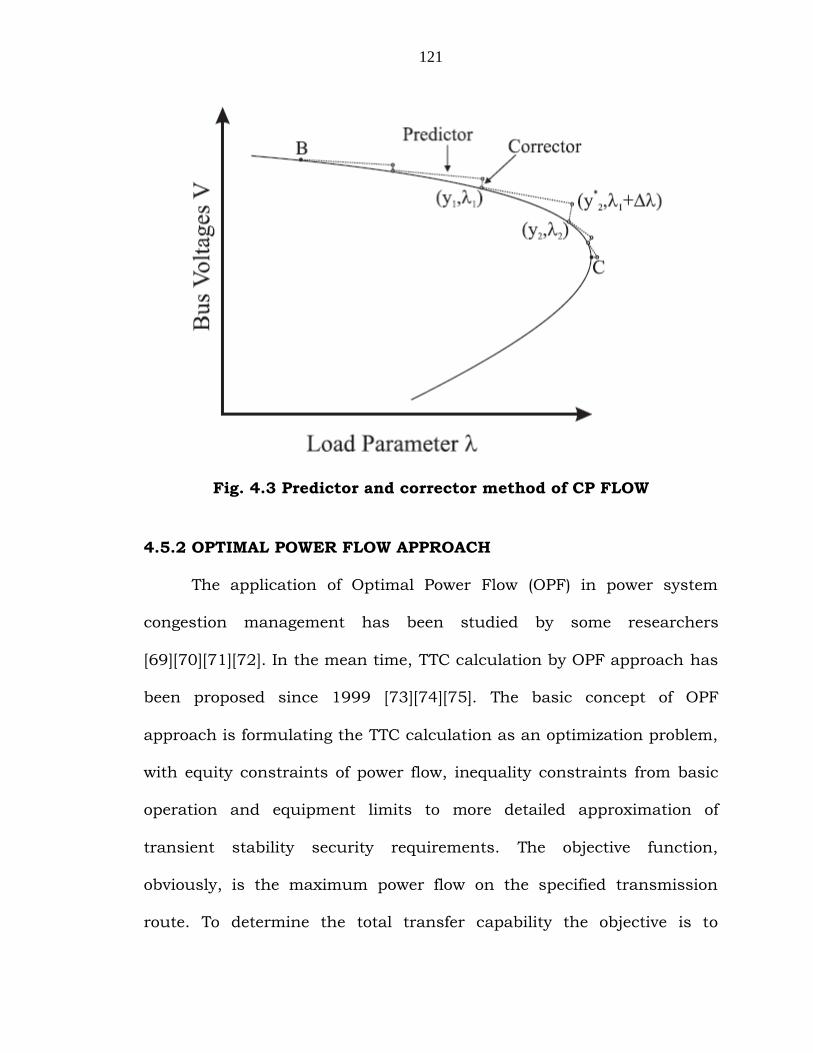
Successive solution of the above equation for different values of
loading parameter λ is obtained by continuation power flow through a
predictor and corrector [65, 66, 68] as shown in Figure 4.3
121
Fig. 4.3 Predictor and corrector method of CP FLOW
4.5.2 OPTIMAL POWER FLOW APPROACH
The application of Optimal Power Flow (OPF) in power system
congestion management has been studied by some researchers
[69][70][71][72]. In the mean time, TTC calculation by OPF approach has
been proposed since 1999 [73][74][75]. The basic concept of OPF
approach is formulating the TTC calculation as an optimization problem,
with equity constraints of power flow, inequality constraints from basic
operation and equipment limits to more detailed approximation of
transient stability security requirements. The objective function,
obviously, is the maximum power flow on the specified transmission
route. To determine the total transfer capability the objective is to
122
maximize the power transfer between the two areas subjected to the
conditions that there is no voltage or thermal or stability limit violations.
Total transfer capability problem formulation can be explained as follows.
Maximize
ij
kji PP (4.8)
Subjected to
0)( ij
jiijijjii CosYVVP (4.9)
0)( ij
jiijijjii SinYVVQ (4.10)
maxmin ggg PPP (4.11)
maxmin ggg QQQ (4.12)
maxijij SS (4.13)
maxmin iii VVV (4.14)
4.5.3 REPEATED POWER FLOW APPROACH
Repeated power flow approach starts from a base case, and
repeatedly solves the power flow equations each time increasing the
power transfer by a small increment until an operation limit is reached
[76]. The advantage of this approach is its simple implementation and
the ease to take security constraints into consideration. In this
dissertation, this method is adopted to solve TTC problem.
123
4.6 ALGORITHM FOR REPEATED POWER FLOW METHOD
In this research work, it is proposed to utilize the repeated power flow
(RPF) method [67] for the calculation of transfer capabilities due to the
ease of implementation. This method involves the solution of a base case,
which is the initial system conditions, and then increasing the transfer.
After each increase, another load flow is solved and the security
constraints tested. Flow chart for the algorithm is given in Annexure IV.
The computational procedure of this approach is as follows:
i. Establish and solve for a base case
ii. Select a transfer case
iii. Solve for the transfer case
iv. Increase step size if transfer is successful
v. Decrease step size if transfer is unsuccessful
vi. Repeat the procedure until minimum step size reached
4.7 AVAILABLE TRANSFER CAPABILITY [ATC]
Available transfer capability computations are essential for
successful implementation of electric power deregulation where power
producers and customers share a common transmission network for
wheeling power from the point of generation to the point of consumption.
The available transfer capability indicates the amount which inter-area
bulk power transfers can be increased without compromising system
security. The value used for available transfer capability affects both
124
system security and the profits made in bulk power transactions.
Moreover, market participants can have conflicting interests in a higher
or a lower available transfer capability. Thus under deregulation, there is
increasing motivation for defensible calculations of available transfer
capability.
4.7.1 IMPORTANCE OF ATC ASSESSMENT
In this present open access or deregulated environment all
the participants (producers and buyers of electrical energy) desire to
produce or consume large amounts of energy and may force the
transmission system to operate beyond one or more transfer limits. This
kind of operation leads to congestion of the system. Therefore accurate
determination of available transfer capability is essential to ensure the
system security and reliability while serving a wide range of bilateral and
multilateral power transactions. The following reasons show the need of
ATC computations
It gives the amount of maximum additional power transfer
between the specified interfaces.
It ensures the secure operation of the system.
On the basis of ATC computation firm and non-firm reservation
of transmission services can be made.
In a deregulated open access market it can be used as tool for
transmission pricing.
125
The limits or binding constraints for ATC can be used in power
system planning and network expansion.
4.8 METHODS OF CALCULATING ATC
As explained above the following methods are used for
determination of ATC
1. Load flow / continuous power flow (CPF) / Repeated Power Flow
(RPF) methods.
2. Optimization based methods
3. Network sensitivity method
Full AC power flow method is the most accurate method for
computation of ATC but its complexity can blot out relationships. The
following linear methods are used for calculation of ATC. Transfer
capabilities can be estimated with simple power system models such as
the DC load flow approximation. A DC model may be preferable to an AC
model particularly in circumstances where the extra data for an AC
model is unavailable or very uncertain, such as the case of very long time
frame analysis.
4.9 COMPUTATION OF ATC USING LINEAR METHODS
In this section linear methods are explained briefly for
determination of available transfer capability followed by the merits and
demerits of these approaches.
126
4.9.1 DC POWER FLOW METHOD
This model assumes that the voltage magnitudes are constant
and only the angles of the complex bus voltage vary. It is also assumed
that the transmission line has no resistance and therefore no losses. In
addition to the speed of computation this method has other useful
properties like linearity and super position.
The following Equation 4.15 explain DC power flow method
ji
ij
ijx
P 1
(4.15)
Where
xij line inductive reactance
θi phase angle at bus i
θj phase angle at bus j
The total power flowing in to bus i is the algebraic sum of generation and
demand at the bus called bus power injection given by Equation 4.16.
j
ji
ijj
ijix
PP 1
(4.16)
This can be expressed in a matrix form by Equation 4.17
n
x
nP
P
..
11
(4.17)
Where the elements of susceptance matrix Bx are functions of line
reactance xij
127
Phase angle of one of the buses is set to zero and eliminating the row and
column from Bx matrix, the reactance matrix can be obtained by
inversion.
The phase angles are obtained as a function of bus injections
as shown in Equation 4.18
1
1
1
1
..
nn P
P
(4.18)
Line flows Pij are obtained from Equation 4.16 to compare with the line
MW limits.
4.9.2 POWER TRANSFER DISTRIBUTION FACTORS
According to power flow point of view power injected in to the
system at a point by generator is extracted by a load at another point
which is known as transaction. Transaction can be found from the linear
property of DC load flow model using sensitivity factor PTDFs [78, 79].
Power transfer distribution factor (PTDF) is defined as the coefficient of
the linear relationship between the amount of a transaction and the flow
on a line. As it relates the amount of one change i.e. transaction amount
to another change i.e. the lone flow. PTDF is the fraction of amount of a
transaction from one zone to another over a specified transmission line.
PTDFij,mn represents the fraction of a transaction from m zone to zone n
that flows over a transmission line connecting zone i to zone j.
128
The Power Transfer Distribution Factor (PTDF) is given by
Equation 4.19
ij
jninjmim
mnijx
XXXXPTDF
, (4.19)
Where
xij transmission line reactance connecting zone i and
zone j
Xim entry in the ith row and mth column of the bus
reactance matrix X
The change in line flow associated with a new transaction is then given
by Equation 4.20.
New
mnmnij
New
ij PPTDFP , (4.20)
4.9.3 LINE OUTAGE DISTRIBUTION FACTORS (LODF)
The simple but most inaccurate method used to calculate the
effect of line outage is DC power flow contingency. The speed of
computation of this method can be improved by using another sensitivity
called line outage distribution factor (LODF). When a line outage occurs
in a system the power flowing on that line is redistributed on to the
remaining lines in the system. This redistribution is measured by LODF
and the fraction of power flowing on the line from zone r to zone s before
it is removed which now flows over a line from zone i to zone j is given by
LODFij,rs.
129
The change in power flow is given by
rsrsijrsij PLODFP ,, (4.21)
rsssrrrsrs
jsjrisir
ijij
rsrs
rsijXXXxN
XXXX
xN
xNLODF
2..
.
.,
(4.22)
Where
xij line reactance connecting zone i and j
Xir entry in the ith row and rth column of the bus reactance matrix
X
Nij number of circuits connecting zone i and zone j
4.10 MAJOR ADVANTAGES & DISADVANTAGES OF THE EARLIER
METHODS:
The advantages and disadvantages of various methods of transfer
capability computation are as follows:
4.10.1 DC APPROXIMATION
The DC approximation is preferred for these reasons:
Fast computation - no iteration.
Thermal limits, MW limits are considered.
Network topology handled with simple and linear methods.
Good approximation over large range of conditions.
Minimum data is required.
But DC approximation is poor for these reasons:
It cannot identify voltage limits
130
It is not accurate when VAR flow and when voltage
deviations are considerable.
Over use of linear superposition increases errors
4.10.2 SENSITIVITY FACTORS
One of the earliest solutions proposed for Available Transfer
capability (ATC) is sensitivity analysis. These sensitivity factors are based
on linear incremental power flow, which are very simple to define and
calculate.
This approach has a major disadvantage that they do not
consider the nonlinear effects of voltage and reactive power. Moreover the
methods based on Power Transfer Distribution Factors (PTDFs) and Line
Outage Distribution Factors (LODFs) can be used to estimate the ATC of
the cases nearer to the base case from which these factors are derived.
4.10.3 OPTIMAL POWER FLOW METHOD
Optimal Power Flow (OPF) and Security Constrained Optimal
Power Flow (SCOPF) are widely used to determine ATC in power corridors
of the system. However these optimization methods are suitable in case
of open access system where there is a possibility of power transactions
occurring from any point to any point.
4.10.4 CONTINUATION POWER FLOW
As discussed earlier this method is initially used for finding
maximum loadability point, however its applications are extended to
131
determine TTC and ATC. The computational time increases due to its
complexity, when contingencies are included.
4.11 ATC COMPUTATION USING COMPLEX VALUED NEURAL
NETWORKS
The practical computations of transfer capability are evolving. The
computations presently being implemented are usually oversimplified
and in many cases do not take sufficient account of effects such as
interactions between power transfers, loop flows, non-linearities,
operating policies and most importantly voltage collapse blackouts. The
transfer capability estimation method proposed by X. Luo et. al. [77] uses
a Multi Layered Feed Forward Neural Networks which is capable of
reflecting variations in load levels and in the status of generation and
transmission lines. The transfer capability was estimated accurately of
between system areas with variations in load levels, in the status of
generation, and in the status of lines. In this work Quick prop algorithm
is used to train the neural network.
The goal of the methods described here is to improve the accuracy
and realism of transfer capability computations. The artificial neural
network approach reported in the methods proposed require a large
input vector for bilateral transaction, so it has oversimplified the
determination of ATC by limiting it to a special case of power transfer to
a single area from all of the remaining areas. Therefore, this method is
unable to track down the bus-to-bus transactions, which is the true
132
spirit of deregulation and nonlinearities of the systems are also not
considered.
4.11.1 ASSUMPTIONS
From the formulations discussed in section 3.4 a Complex Valued
Neural Network approach is implemented for ATC computation.
The following assumptions are made while calculating the ATC.
a) The base case power flow of the system is feasible and
corresponds to a stable operating point;
b) The load and generation patterns vary very slowly; and
c) TTC calculation is in the steady state analysis domain.
4.12 COMPUTATION OF ATC FOR A 9-BUS SYSTEM
For computing Available Transfer Capability using the proposed
approach a 9 bus system [120] is considered (Annexure – 1). It has 3
generator buses and the number of transmission lines is 9 as shown in
Figure 4.4.
This method involves the solution of a base case, which is the
initial system conditions, and then increasing the transfer. After each
increase, another load flow is solved and the security constraints tested.
Voltage constraint is taken
133
Fig. 4.4 Nine bus system.
The system divided in to two areas. Area 1 comprises of bus 1,bus
3,bus 4, bus 5 and bus 6 where as area 2 comprises of the remaining
buses as shown in Fig. 4.4 [84]. The tie lines between the two areas are
line 4-9 and line 6-7. These lines transmit the power from one
geographical area to other area.
134
4.12.1 LEARNING METHODOLOGY
Learning methodology uses complex back propagation algorithm
explained in Chapter 3. Repeated power flow method is utilized to
generate training patterns using Newton Raphson load flow method.
Repeated power flow (RPF) method is proposed for calculating ATC due to
the ease of implementation. In this method the available transfer
capability (ATC) from one bus/area/zone to another bus/area/zone can
be found by varying the amount of transaction until one or more line
flows in the transmission system considered or a bus voltage reaching
the limiting value. The proposed new methodology is based on the full Ac
load flow and strong generalization capability of complex neural network
offers a great potential for real time evaluation of ATC incorporating load
variation, effect of reactive power loss of the system.
For calculating ATC using Repeated Power Flow (RPF) method the
following choices are made:
Establish a secure, solved base case.
Specify a transfer including source and sink assumptions.
Identify the branch flows influencing the ATC of selected branch
appreciably.
Identify the line outages having significant influence on the above
said branch power flows.
135
Generate numerous training data sets involving above said power
flows and line outages.
The transfer margin is the difference between the transfer at the
base case and the limiting case.
The flow chart for the above algorithm is shown in Annexure –IV.
The calculation of ATC is done by using the Newton Raphson load flow
solution to compute the power flow of each transfer case. This method is
less prone to divergence with ill-conditioned problems. And also the
number of iterations required is independent of the system size. The
loads at bus number 7 and 9 are increased simultaneously and the
transfers from area 1 to area 2 are obtained. The total transfer capability
is the sum of transfers through the interconnecting lines i.e. line joining
buses 4 and 9, buses 6 and 7. The available transfer capability is given
by Equation 4.23
ATC = TTC – base case transfer (4.23)
Satisfying the following system operating conditions
Nj
ijijijji CosYVVPi
0)( (4.24)
Nj
ijijijji SinYVVQi
0)( (4.25)
maxmin ggg PPP (4.26)
maxmin ggg QQQ (4.27)
max,min, iii VVV (4.28)
136
0 50 100 150 200 2500.65
0.7
0.75
0.8
0.85
0.9
0.95
1
1.05
Load in area 2 (MW)
Voltage
Bus 7
Bus 9
Load at Bus 5 is 90+j30
Fig. 4.5 P-V curves with load 90+j30
The above Figure 4.5 shows the P-V curve obtained from
repeated power flow. The load in area 1 that is at bus 5 is maintained as
90+j30 where as the load in area 2 that is at bus 7 and bus 9 is varied
slowly. It is assumed that bus 7 and bus 9 are critical buses compared
to other buses and the voltage collapse points of these buses are shown
with respect to the total load in area 2. From the results obtained from
the repeated power flow it is observed that the voltage at these two buses
reached the nose point compared to other buses.
137
0 20 40 60 80 100 120 140 160 180 2000.65
0.7
0.75
0.8
0.85
0.9
0.95
1
1.05
Load in area 2 (MW)
Voltage
Bus 7
Bus 9
Load at Bus 5 is 120+j40
Fig. 4.6 P-V curves with load 120+j40
Figure 4.6 represents the P-V curve without considering the
contingencies. To show the effect of change of load in one area on the
voltage profile these curves are plotted at different loads. In this case the
load is taken as 120+j40 at bus 5 of area one.
138
0 20 40 60 80 100 120 140 160 180 2000.65
0.7
0.75
0.8
0.85
0.9
0.95
1
1.05
Load in area 2 (MW)
Vola
tge
Bus 7
Bus 9
Load at Bus 5 is 150+j50
Fig. 4.7 P-V curves with load 150+j50
In figure 4.7 variations in voltage is plotted at a different load
of 150+j50 in area 1. It is observed that at a lesser value of the
convergence is ceased as shown which will also affect the transfer
capability of the system. It is observed that the there is an
interaction between the power transfers and variation of load. It is
also observed that there is a certain change the load margin due to
which the transfer capability also changes.
139
0 20 40 60 80 100 120 1400.7
0.75
0.8
0.85
0.9
0.95
1
1.05
Load in area 2 (MW)
Voltage
Bus 7
Bus 9
Load at Bus 5 is 90+j30
Fig. 4.8 P-V curves with line outage 4-5
In Figure 4.8 the bus voltages at bus 7 and bus 9 are plotted using
RPF method considering a single contingency with line outage 4-5. The
load in area 1 is maintained at 90+j30. When compared with the Figure
4.7, for the same load in area 1 there is large change in load power
margin and hence the transfer capability also. The graphical
representation of change in ATC is shown in Fig. 4.10 and Fig. 4.11.
140
0 20 40 60 80 100 120 140 160 1800.7
0.75
0.8
0.85
0.9
0.95
1
1.05
Load in area 2 (MW)
Voltage
Bus 7
Bus 9
Load at Bus 5 is 90+j30
Fig. 4.9 P-V curves with line outage 5-6
The single contingencies considered in Figure 4.9 is outage of
line connecting bus 5 and bus 6 in area 1. It can be observed that the
voltage collapse at bus 7 and bus 9 at a lower value of load compared to
that of contingency free system.
141
80 100 120 140 160 180 200 220200
225
250
275
300
325
350
375
400
425
450
Load in area 1 (MW)
AT
C (
MW
)
Fig. 4.10 Effect of change in load on ATC without contingency
Figure 4.10 represents the variation of available transfer
capability with respect to the change in load in area 1. The load in area 1
is changed with constant power factor. As the load is increased the ATC
from are 1 to area 2 is decreased due to decrease in load margin. No
contingencies are considered here.
142
80 100 120 140 160 180 200 22050
55
60
65
70
75
80
85
90
95
100
Load in area 1 (MW)
AT
C (
MW
)
Fig. 4.11 Effect of change in load on ATC with contingency
The variations in ATC with respect to the changes in load of area 1
with contingency i.e. removing line 4-9 are shown in Figure 4.11.
The number of training samples is 40 which are used for training
the network. These training samples are obtained from repeated load flow
method at different load patterns and two single line outages. The
proposed network accepts the diagonal elements of bus admittance
matrix to map the contingencies and load in area 1 as inputs, the
available transfer capability in complex form is the output. This method
is proposed for better prediction how a realistic power system will react
143
over a wide range of operating conditions. The variation of error with
respect to number of iterations is shown in Figure 4.12.
0 1 2 3 4 5 6 7
x 104
0
0.05
0.1
0.15
0.2
0.25
0.3
Iterations
Erro
r
Figure 4.12 Error plot
4.12.2 RESULTS AND DISCUSSIONS
For the purpose of verifying the validity and correctness of the
proposed method a 9 bus system is selected to compute the real and
reactive power transfer from one area to another area. The system
consisting of 9 buses is divided in to two areas. The complex load levels
144
used to create data for training the proposed neural network in area 1
are varied from 100% to 250% of base case values using different line
outages. The available transfer capability (ATC) in MW and the reactive
power transfers in MVAR at different test cases are computed. The
comparison between the proposed CVNN method and the repeated power
flow (RPF) methods are shown in Tables 4.1 to 4.4.
Table 4.1: Power transfer and ATC without contingency
Load in
area 1 RPF CVNN
ATC
(MW)
90+j30 438+j276 441+j282 441
120+j40 416+j245 418+j244 418
150+j50 393+j221 385+j224 385
180+j60 365+j190 359+j180 359
210+j70 340+j175 332+j168 332
Table 4.2: Power transfer and ATC with Line 5-6 outage
Load in
area 1 RPF CVNN
ATC
(MW)
90+j30 357+j214 351+j211 351
120+j40 344+j203 338+j210 338
150+j50 323+j77 318+j95 318
180+j60 287+j130 284+j133 284
210+j70 210+j40 204+j42 204
145
Table 4.3: Power transfer and ATC with Line 6-7 outage
Load in
area 1 RPF CVNN
ATC
(MW)
90+j30 298+j192 290+j186 290
120+j40 293+j185 284+j182 284
150+j50 290+j186 281+j179 281
180+j60 282+j175 276+j172 276
210+j70 244+j260 239+j256 239
Table 4.4: Power transfer and ATC with Line 9-4 outage
Load in
area 1 RPF CVNN
ATC
(MW)
90+30j 90+j34 92+j35 92
120+j40 86+j38 86+j33 86
150+j50 80+j16 81+j20 81
180+j60 78+j20 76+j22 76
210+j70 73+j25 75+j21 75
It is observed that some outages cause a large change in
power transactions as shown in Table 4.3 and Table 4.4. This is due to
the voltage violation limits of the system. The results are compared and it
is found that transfer capability is reduced by 70% in case of
contingency.
146
4.13 COMPUTATION OF ATC FOR A 30 BUS SYSTEM
In this case IEEE 30 bus system Fig. 4.13 [77] (Annexure – 1)
is considered for calculation of Available Transfer Capability. There are
three areas which are interconnected through tie lines as shown in table
4.5 and 4.6.
Table 4.5: Areas
Table 4.6: Tie Lines
The power transferred between one area to other area is the sum of the
powers transferred through the tie lines connecting the two areas. The
available transfer capability between the areas can be found using the
Equation 4.29. Repeated Power flow method discussed in section 4.10.2
is used to obtain the voltage constrained transfer capability of the
system. The load in one area is varied in steps until Jacobian becomes
singular and a point of voltage collapse is reached. In this case Bus 18,
Bus 19 and Bus 20 are assumed to be critical buses according to voltage
profiles and the P-V curves obtained from RPF solution are plotted.
Area Bus Numbers
1 1,2,3,4,5,6,7,8,9,11 & 28
2 12,13,14,15,16,17,18,19,20 & 23
3 10,21,22,24,25,26,27,29 & 30
Areas Tie Lines
Area 1 – Area 2 Bus 4 – Bus 12
Area 1 – Area 3
Bus 6 – Bus 10
Bus 9 – Bus 10
Bus 28 – Bus 27
147
Fig. 4.13 IEEE 30 Bus system
148
75 80 85 90 95 100 105
0.65
0.7
0.75
0.8
0.85
0.9
0.95
1
Load in area 2 (MW) with p.f 0.8
Voltage
Bus 20
Bus 19
Bus 18
Fig. 4.14 P-V curves
4.13.1 RESULTS AND DISCUSSIONS
The voltage constrained transfer capability is calculated using
repeated power flow (RPF). The voltages at bus 18, 19 and 20 are
considered to be critical and the voltage collapse points are shown in
Figure 4.14. The Load in area 3 is maintained at 48.5+j25 where as the
load in area 2 is varied in small steps while the power factor is
maintained constant at 0.8.
149
76 78 80 82 84 86 88 90 92 940.7
0.75
0.8
0.85
0.9
0.95
1
Load in Area 2 (MW) with p.f 0.75
Voltage
Bus 20
Bus 19
Bus 18
Fig. 4.15 P-V curves
In the above Figure 4.15 the power factor maintained at 0.75
where as the area 3 load is changed to 210+j157.88. It can be observed
that the voltage constrained total transfer capability is lesser compared
to that with lesser power transaction.
150
75 80 85 90 95 100 1050.65
0.7
0.75
0.8
0.85
0.9
0.95
1
Load in area 2 (MW) with p.f 0.82
Voltage
Bus 20
Bus 19
Bus 18
Fig. 4.16 P-V curves
The above Figure 4.16 shows the variation in bus voltages with the
change in load of area 2 keeping the Area 3 load as 138.5+j103.8.
In this case the number of input patterns is reduced to two. The
power factor of the load in area 2 and the load in area 3 are considered
as inputs to observe the effect of load power factor in one area and
change in real and reactive powers in another area.
151
The values of ATC estimated by using the load and power factor
reduce the number of input neurons and very much useful for large
systems. No contingencies are considered in this case. In case of
contingencies the method used in the previous section can be used.
Table 4.7: ATC with varying Load in area 3
P.F Load in Area 3 ATC1-2 (RPF) ATC1-2 (CVNN) ATC1-3 (RPF) ATC1-3 (CVNN)
0.8 138.5+j103.8 149 152 250 245
0.8 168.5+j126.3 151 150 260 258
0.8 198.5+j148.8 152 145 265 267
0.8 210.5+j157.8 151 144 268 270
In Table 4.7 The effect of change in load i.e. real and reactive power
in area 3 on the transfer capability is shown. It is observed that the
increase in load has a noticeable effect on the available transfer
capability from area 1 to 2 and also from area 1 to 3. In this case the
power factor is maintained constant while the load is varied in steps.
Table 4.8: ATC with constant Load in area 3 and variable P.F
P.F Load in Area 3 ATC1-2 (RPF) ATC1-2 (CVNN) ATC1-3 (RPF) ATC1-3 (CVNN)
0.78 210.5+j157.8 150 148 267 272
0.8 210.5+j157.8 152 150 271 274
0.82 210.5+j157.8 153 150 274 278
0.86 210.5+j157.8 153 152 277 278
152
Table 4.8 shows the variation of ATC with respect to power factor
and at a constant area load. There is a very small effect on ATC in this
case. The result obtained using the proposed method is compared with
the standard RPF method.
4.14 CONCLUSIONS
This chapter introduces the application of complex valued neural
network for ATC computations with and without contingencies. To
evaluate the performance a numerical example of 9 bus test system is
presented. The voltage limits of the buses and the line losses are well
considered in this method. It is observed that, using this method
available transfer capabilities between system areas can be estimated
accurately with variations in load levels, in the status of lines. The
simulation results show that the proposed method is very effective in
determining the ATC. The suitability of this method is also demonstrated
by taking IEEE 30 bus system where the number of inputs are reduced
to allow the on line computations of ATC for a larger system. In this
problem it is observed that as the number of inputs mapping the
nonlinear system output decreases the relative error increases. In a
deregulated environment, the power transaction between one area to
other area can occur only when there is adequate ATC available for that
interface to ensure system security. This available transfer capability
(ATC) information is to be continuously updated and made available to
153
all participants of the energy market through Open Access Same Time
Information System (OASIS). For such type of n line applications the
proposed method is suitable as it makes use of repeated power flow
method based on Newton-Raphson formulation and the good
generalization capability of the complex valued artificial neural networks.
The main conclusions of this work are:
The proposed CVNN method is effective in calculating the
ATC between different areas subject to system operating
limits;
This method can be adopted for computation of ATC with
constant load power factor at different power factors of the
load; and
The application of proposed method can also be extended to
determine the variations in ATC with respect to reactive