1 Computation of Incompressible and Weakly-Compressible Viscoelastic Liquids Flow: finite element/volume schemes M. F. Webster * , I. J. Keshtiban, and F. Belblidia Institute of Non-Newtonian Fluid Mechanics, Department of Computer Science, University of Wales, Swansea, SA2 8PP, UK. * Author for correspondence. Email: [email protected]
Transcript
1
Computation of Incompressible and Weakly-Compressible
In our previous studies [14,34], we have developed a numerical scheme for Newtonian and
viscoelastic weakly-compressible liquid flows based on a pure finite element (fe)
methodology. There, we demonstrated the capability of this method to deal with complex
flows. In this article, we introduce a hybrid finite element/finite volume (fe/fv) algorithm to
handle such flows at low Mach number (Ma) and Reynolds number (Re) under isothermal
conditions. The finite volume (fv) sub-cell scheme is incorporated for the hyperbolic
constitutive equation, considered here of Oldroyd-B form. This model provides a constant
shear viscosity and strain-hardening (unbounded) properties in extension. The
continuity/momentum balance is accommodated through a semi-implicit fractional-
staged/pressure-correction fe-formulation.
Compressibility effects are characterised by the Mach number, the ratio of the speed of
fluid flow (u) to the speed of sound (c). The incompressible limit of a compressible flow is
obtained, under suitable constraints on length and time scales, when the Mach number
asymptotes to zero (Ma≈0) [21]. Low Mach number (LMN) flows may arise for either liquid
or gas material states, with dependency on physical conditions. Liquid materials are
frequently considered as incompressible, as density tends to reflect a weak functional
dependence upon pressure. Therefore, such flows may reflect the influence of compressibility
under expose to high pressure-differences, particularly for highly viscous/viscoelastic
materials, or in instances such as liquid impact or jet cutting.
LMN flow computations remain a significant challenge, notwithstanding the success of
some compressible flow solvers in simulating many complex compressible flows. Many
numerical methods encounter severe difficulties when dealing with instances where Ma<0.3
[35], where deterioration of efficiency and accuracy are experienced. One of the key
difficulties arises from the fact that the governing equation system switches in type. The
equations for viscous compressible flow form a hyperbolic-parabolic system of finite wave-
speeds (inviscid case, hyperbolic), whilst those for incompressible viscous flow assume an
elliptic-parabolic system with infinite propagation rates. This is augmented for viscoelastic
flows by a sub-system of hyperbolic form. The lack of efficiency in solving the compressible
equations for LMN is associated with large disparity in wave speeds across the system [35],
see Appendix for more detail.
There is significant interest in developing numerical algorithms to deal with LMN flows
for viscoelastic liquid flows, where Ma approaches zero. LMN flows adopt an important role
in nature and industrial processing. In many technical applications, liquid flow can
demonstrate significant compressibility effects. This would include examples of: injection
molding, high-speed extrusion, jet cutting, liquid impact, and under recovery of and
4
exploration for petroleum. Under such circumstances, the compressibility of viscoelastic
liquids should be taken into account, in order to accommodate typical flow phenomena
arising, say cavitation [6] or flow instabilities [10]. In capillary rheometry, compressibility
effects may be significant and have a major impact upon the time-dependent pressure changes
in the system [17]. If numerical simulations are to prove accurate, such physics must be
accounted for.
There are two major computational approaches adopted to solve LMN flows: pressure-
based methods (incompressible solvers) and density-based methods (compressible solvers).
With pressure-based methods pressure is a primitive variable and density a dependent
variable. The first implementation of pressure-based schemes for compressible LMN flows
may be attributed to Harlow and Amsden [12]. The use of pressure as a primary variable
allows computation to remain tractable over the entire spectrum of Mach numbers. This is due
to the fact that pressure changes remain finite, irrespective of prevailing Mach Number [13].
Moreover, extension of these method to compressible flows retains robustness [21]. On the
other hand, with density-based methods, continuity provides an equation for density, and
pressure is obtained from an equation of state. In pressure-based methods, continuity is
utilized as a constraint on velocity and is combined with momentum to form a Poisson-like
equation for pressure. These two approaches are quite different, with respect to their choice
of variables, sensitivity to numerical stability and choice of solvers [19]. Since our
constructive formalism emanates from incompressible flow, it is natural for us to consider
pressure-based methods. In addition, the vast majority of incompressible viscoelastic schemes
are pressure-based, and on such grounds, may be preferred for algorithmic development.
In the fe-context, based on the ideas of Van Kan [31], Townsend and Webster [28]
introduced a second-order Taylor-Galerkin/pressure-correction (TGPC) scheme. This
fractional-staged formulation introduced an operator-splitting stencil of predictor-corrector
structure, significantly reducing computational overheads. In this manner, solutions have been
derived previously for incompressible viscoelastic flows [7,18]. Under the TGPC scheme, fe-
treatment of the constitutive equations incorporates consistency through Taylor-Petrov-
Galerkin streamline upwinding (TSUPG), with recovery applied upon velocity gradients [18].
In the fv-context, Webster and co-workers [1-3] have advanced an alternative spatial
discretisation, via a novel hybrid fe/fv-scheme for steady incompressible viscoelastic flows.
With this methodology, the constitutive equation is accommodated via a sub-cell cell-vertex
fv-algorithm. The main philosophy here is to apply fe-stencils to the self-adjoint component of
the system, and fv-forms to the hyperbolic sections. The above studies are concerned with
incompressible flow considerations.
With compressible flow in mind, Webster and co-workers [14,34] have already provided
extension to the ‘pure fe’ TGPC algorithm, handling weakly-compressible viscous-
5
viscoelastic liquid flows at LMN, termed C-TGPC (Compressible-TGPC). Under such
setting, the divergence-free condition applicable for incompressible flow, is replaced with the
continuity equation for compressible liquid flow. The temporal derivative of density is
interpreted through pressure representation, via an equation of state. For this purpose, two
discrete representations have been proposed to interpolate density: a piecewise-constant form
with gradient recovery and a linear interpolation form, similar to that on pressure. Both
density interpolations provide identical solutions. The piecewise-constant interpolation
scheme is selected for its advantages of order retention and efficiency in implementation.
Previously, this pure fe-implementation has been successfully tested on a number of standard
benchmark problems. Consistency has been realised in simulating compressible flows
(Ma<0.3), as well as almost incompressible liquid flows (Ma≈0). As such, enhanced
convergence properties have been gathered compared to the original TGPC algorithm. In
addition, in the present study we are interested in advancing the hybrid formulation, via
embedding compressibility considerations, leading to a compressible hybrid fe/fv-
implementation.
The present article is organized as follows: the governing equations for compressible
viscoelastic flow are expounded in Section 2. In Section 3, we introduce the fractional
equation stages of the viscoelastic pressure-correction scheme, outlining the spatial
discretization strategies employed as necessary. In Section 4, we present the application of
our methodology to the 4:1 contraction flow test-problem. A continuation solution strategy,
through increasing Weissenberg number (We), is adopted in seeking steady-state solutions.
Throughout the study, we conduct comparison across scheme variants and flow settings,
drawing upon the literature. The schemes proposed are validated for consistency and accuracy
at a fixed level of We=1.5. This is followed by analysis up to critical levels of Weissenberg
number. Differences due to inclusion of compressibility effects and inertia are highlighted
through flow patterns and vortex activity.
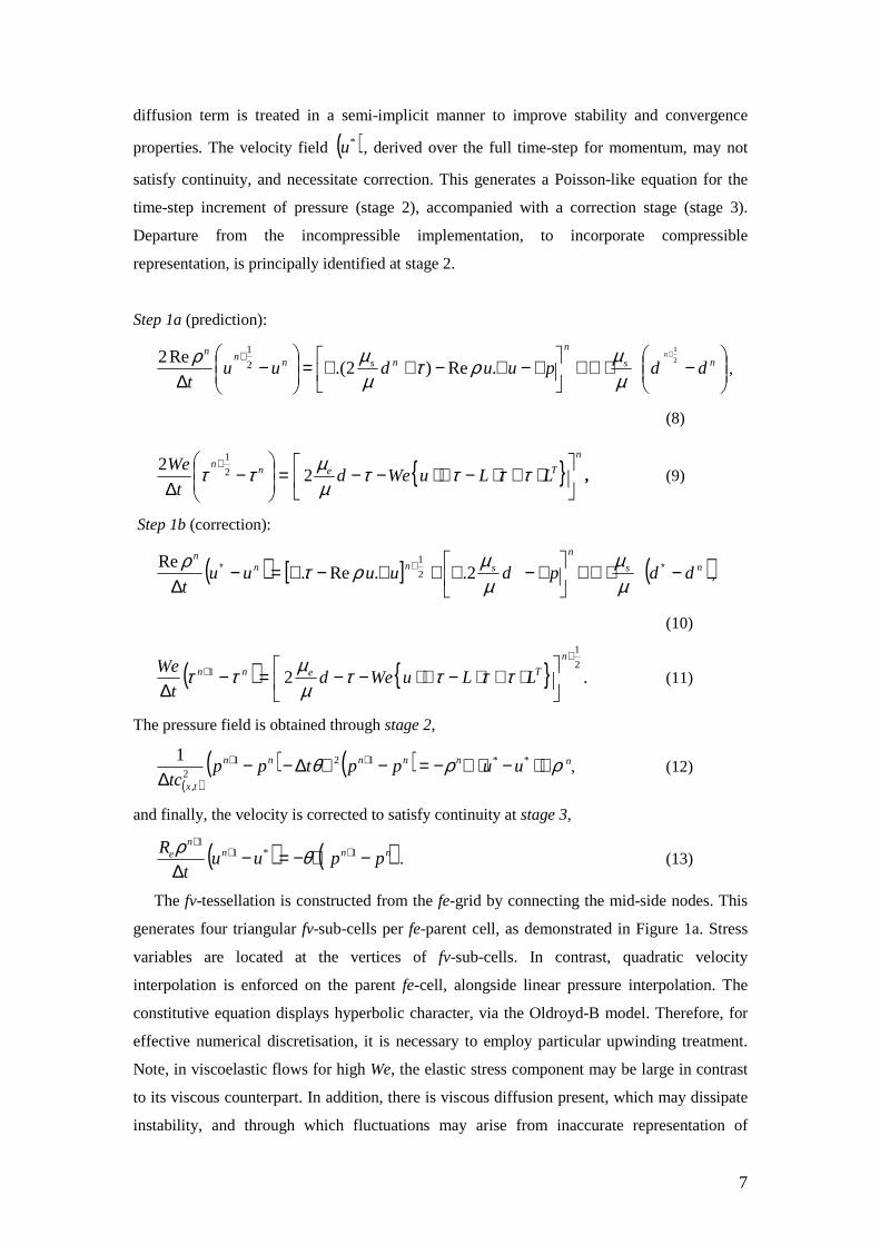
2. Governing equations
For compressible viscoelastic flow, the governing non-dimensional equations for
conservation of mass, momentum, and the development of stress may be expressed as:
( ) 0=⋅∇+∂∂
ut
ρρ, (1)
puudt
u s ∇−∇⋅−
+⋅∇=∂∂ ρτ
µµρ Re2Re . (2)
The constitutive state law for an Oldroyd-B model fluid is expounded, viz.
6
( ) τµµττττ −+⋅+⋅+∇⋅−=
∂∂ eTLLWeWeu
tWe 2 . ( 3)
Here,ρ ,u , p ,τ represent fluid density, velocity vector, pressure and extra-stress tensor
respectively; ( ) 3/2/ ijTij
Tijijij LLLd δ−+= represents an augmented rate-of-deformation tensor
and uLT ∇= , the velocity gradient. The total viscosity, µ splits into Newtonian (solvent)
viscosity, sµ , and elastic (polymeric), eµ , components, such that se µµµ += . Here, we take
91=µµs . Non-dimensional group numbers, of Reynolds and Weissenberg numbers, are
defined as:
µρ oUL=Re ,
oeL
UW
λ= (4)
where,λ is a relaxation time, U a characteristic velocity (averaged at outlet) and oL is a
length-scale (channel-exit half-width). To complete the set of governing equation, it is
necessary to introduce an equation of state to relate density to pressure. Here, we employ the
modified Tait equation of state [27], a well-established formulation for liquids,
m
Bp
Bp
=
++
00~~
ρρ
, with augmented pressure
+−= dtracepp s
µµτ 2
31~ . (5)
Parameters B and m are constants†, and 0~p , 0ρ denote reference scales for pressure and
density. Assuming isentropic conditions (see [13]), and employing the differential chain rule,
we gather,
( ) t
p
ct
p
pt tx ∂∂=
∂∂
∂∂=
∂∂
2,
1ρρ, (6)
( )( )2
,
~
txcBPmp =+=
∂∂
ρρ, (7)
where, ( )txc , introduces the speed of sound, a field variable, distributed in space and time.
3. Numerical Discretisation
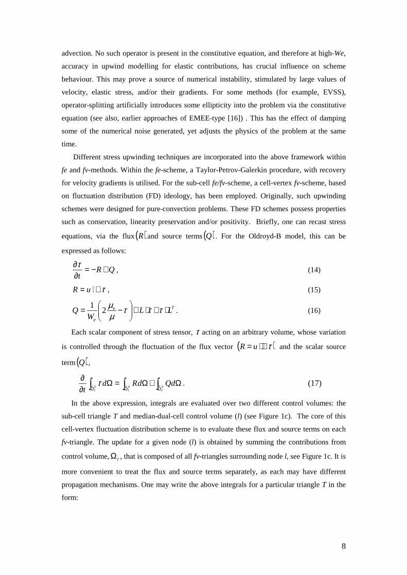
The C-TGPC scheme is a time-stepping procedure of multiple fractional-staged equations.
The pressure-correction procedure accommodates the continuity constraint to second-order
accuracy in time, introducing a three-staged structure per time-step cycle (see [28,30]). At
stage one, a predictor-corrector equation doublet, provides velocity and stress fields, predicted
at the half time-step ( ) 2
1
, +nu τ and corrected for the full time-step ( ) 1* ,+n
u τ . The momentum
† Generally, B and m are functions of temperature.
7
diffusion term is treated in a semi-implicit manner to improve stability and convergence
properties. The velocity field ( )*u , derived over the full time-step for momentum, may not
satisfy continuity, and necessitate correction. This generates a Poisson-like equation for the
time-step increment of pressure (stage 2), accompanied with a correction stage (stage 3).
Departure from the incompressible implementation, to incorporate compressible
representation, is principally identified at stage 2.
Step 1a (prediction):
−⋅∇+
∇−∇−+∇=
−
∆
++ns
n
nsnnn
ddpuuduut
n2
1
.Re)2.(Re2
2
1
µµρτ
µµρ
,
(8)
n
Tenn
LLuWedt
We
⋅+⋅−∇⋅−−=
−
∆+
ττττµµττ 2
2 2
1
, (9)
Step 1b (correction):
( ) [ ] ( )ns
n
snnn
ddpduuuut
−⋅∇+
∇−∇+∇−∇=−∆
∗+∗
µµ
µµρτρ
2..Re.Re
2
1
,
(10)
( ) 2
1
1 2+
+
⋅+⋅−∇⋅−−=−∆
n
Tenn LLuWedt
We ττττµµττ . (11)
The pressure field is obtained through stage 2,
( )( ) ( ) ρρθ ∇⋅−⋅∇−=−∇∆−−
∆++ **121
2,
1uupptpp
tcnnnnn
tx
n, (12)
and finally, the velocity is corrected to satisfy continuity at stage 3,
( ) ( )nnnn
e ppuut
R −∇−=−∆
+++
1*11
θρ. (13)
The fv-tessellation is constructed from the fe-grid by connecting the mid-side nodes. This
generates four triangular fv-sub-cells per fe-parent cell, as demonstrated in Figure 1a. Stress
variables are located at the vertices of fv-sub-cells. In contrast, quadratic velocity
interpolation is enforced on the parent fe-cell, alongside linear pressure interpolation. The
constitutive equation displays hyperbolic character, via the Oldroyd-B model. Therefore, for
effective numerical discretisation, it is necessary to employ particular upwinding treatment.
Note, in viscoelastic flows for high We, the elastic stress component may be large in contrast
to its viscous counterpart. In addition, there is viscous diffusion present, which may dissipate
instability, and through which fluctuations may arise from inaccurate representation of
8
advection. No such operator is present in the constitutive equation, and therefore at high-We,
accuracy in upwind modelling for elastic contributions, has crucial influence on scheme
behaviour. This may prove a source of numerical instability, stimulated by large values of
velocity, elastic stress, and/or their gradients. For some methods (for example, EVSS),
operator-splitting artificially introduces some ellipticity into the problem via the constitutive
equation (see also, earlier approaches of EMEE-type [16]) . This has the effect of damping
some of the numerical noise generated, yet adjusts the physics of the problem at the same
time.
Different stress upwinding techniques are incorporated into the above framework within
fe and fv-methods. Within the fe-scheme, a Taylor-Petrov-Galerkin procedure, with recovery
for velocity gradients is utilised. For the sub-cell fe/fv-scheme, a cell-vertex fv-scheme, based
on fluctuation distribution (FD) ideology, has been employed. Originally, such upwinding
schemes were designed for pure-convection problems. These FD schemes possess properties
such as conservation, linearity preservation and/or positivity. Briefly, one can recast stress
equations, via the flux( )R and source terms( )Q . For the Oldroyd-B model, this can be
expressed as follows:
QRt
+−=∂∂τ
, (14)
τ∇⋅= uR , (15)
Te
e
LLW
Q ⋅+⋅+
−= τττµµ
21
. (16)
Each scalar component of stress tensor, τ acting on an arbitrary volume, whose variation
is controlled through the fluctuation of the flux vector ( )τ∇⋅= uR and the scalar source
term( )Q ,
∫∫∫ ΩΩΩΩ+Ω=Ω
∂∂
Tl
Tl
Tl
QddRdt ˆˆˆ
τ . (17)
In the above expression, integrals are evaluated over two different control volumes: the
sub-cell triangle T and median-dual-cell control volume (l) (see Figure 1c). The core of this
cell-vertex fluctuation distribution scheme is to evaluate these flux and source terms on each
fv-triangle. The update for a given node (l) is obtained by summing the contributions from
control volume, lΩ , that is composed of all fv-triangles surrounding node l, see Figure 1c. It is
more convenient to treat the flux and source terms separately, as each may have different
propagation mechanisms. One may write the above integrals for a particular triangle T in the
form:
9
TlMDCT
Tl
nl
nlT
l QRt
+=∆−
Ω+
αττ 1
ˆ , (18)
where, TlΩ is the area of the median dual cell (MDCT) associated with node (l) within
the triangle T. To accommodate upwinding, the flux term RT is calculated over
triangle T, and is distributed over the vertex nodes based on flow direction and
coefficientsα . Here, for node (l), Tlα designates the contribution to node (l) from flux
RT on triangle T. A key feature of the cell-vertex fv-method lies within the definition
of -coefficients. Webster and co-workers [2,3] found the Low Diffusion B (LDB) scheme
appropriate, for steady viscoelastic flows where source terms may dominate. This is a linear
scheme with linearly preservation properties and second-order accuracy [3]. It conveys a
relatively low-level of numerical diffusion in comparison to a linear positive scheme. The
LDB distribution coefficients iα are obtained on each triangle via angles 21,γγ (see Figure
1b), subtended at an inflow vertex (i) by the advection velocity a (average of velocity field
per fv-cell), viz.
( )21
21
sin
cossin
γγγγα
+=i , ( )21
12
sin
cossin
γγγγα
+=j , 0=kα . (19)
Note, when 1γ is larger than 2γ , then iα is larger than jα , and hence by design, node (i) gains
a larger contribution from the flux than node (j).
The flux TR and the source lMDCQ terms, as evaluated in Eq.(18) over different control
volumes, create some inconsistency introducing inaccuracy even for simple model problems.
To rectify this position, Wapperom and Webster [32] proposed a generalised formulation that
consistently distributes both flux and source terms over the fv-triangle, viz.,
( ) ( ) ( )lMDC
lMDCMDCTT
TlT
nl
nl
Tl
TTTQRQR
t+++=
∆−Ω +
δαδττ 1ˆ. (19)
The parametersTδ and MDCδ are applied to discriminate between various update strategies,
being functions of fluid elasticity, velocity field and mesh size. By appropriate selection of
Tδ and MDCδ , one can obtain various blends for different flow regimes. With
( )haWefT ,,=δ and 1=MDCδ , the nodal update is similar to consistent streamline
upwinding, as used in fe-schemes. We follow [2,3,32] such that 1=MDCδ and 3/ξδ =T , if
3≤ξ and 1 otherwise. Here, ( )haWe /=ξ , with a the magnitude of the advection velocity,
averaged per fv-cell and h is a mesh-size scale (square-root of the fv-cell size). Subsequently,
10
Aboubacar [1-3] proposed a method with appropriate area weighting to enforce time
consistency,
( ) ( ) ( )MDC
T
lMDC
lMDCMDC
FD
T TTTlT
nl
nl TTT
QRQR
t Ω+
+Ω
+=
∆− ∑∑ ∀∀
+ δαδττ 1
, (20)
where, ∑ Ω=ΩlT T
TlTFD αδ and ∑ Ω=Ω
l TMDC
TlMDCMDC δ .
4. Discussion of results
Flow through an abrupt contraction for an Oldroyd-B fluid is well-documented in the
literature, where it is recognised as a valuable benchmark problem, useful to qualify
numerical stability of schemes at high We-levels. It is a natural choice in this study for two
principal reasons. First, from a numerical point of view, it presents a relatively simple
geometric configuration, generating complex shear and extensional deformation, allowing a
framework to investigate numerical schemes for complex viscoelastic flows. Second, from a
practical standpoint, its relevance arises in several polymeric processing applications, such as
in injection molding, extrusion and rheometry itself.
4.1. Literature review
A challenging feature of the abrupt contraction (non-smooth) flow problem is the presence of
a stress singularity at the re-entrant corner, which impacts upon stability properties of
numerical schemes. Many fluid models suffer a limiting Weissenberg number (We), beyond
which numerical solutions fail. This issue has become known as ‘the high We problem-
HWNP’ [15], drawing considerable attention over the last two decades or so. In the
incompressible context, and commenting upon our own contributions, one may site those
based on the ‘pure’ fe-framework, from Carew et al., [7] and Matallah et al., [18], providing
literature reviews and consensus findings on vortex behaviour. Subsequently, Wapperom and
Webster [32] introduced a hybrid fe/fv-methodology. This was developed further in
Aboubacar and Webster [1]. There, mesh refinement was conducted for an Oldroyd-B model.
Extension of this work in Aboubacar et al., [2,3], focused on alternative geometries (planar
and axisymmetric, sharp- and rounded-corners) and several viscoelastic models (Oldroyd-B
and PTT-variants). An overview of experimental and numerical studies was also documented
there.
Elsewhere, Guénette and Fortin [11] proposed a stable and cost-effective mixed fe-method,
a variant of the EVSS formulation. Numerical results were presented for the PTT fluid model.
Yurun [37] compared two variants of EVSS fe-schemes on this benchmark problem
(discontinuous Galerkin DG and continuous SUPG). The DG/EVSS scheme was observed to
reflect significant improvement over the SUPG/EVSS variant at higher We-levels
11
(smoothness in solutions and enhanced robustness, see on for fv-solutions). The above subject
matter is covered in the comprehensive literature review of Baaijens [5].
In the context of fv-formulations, Phillips and Williams [23,24] investigated the
differences in vortex structure and development, with and without inertia. This work covered
planar and axisymmetrical configurations, and was based on a semi-Lagrangian fv-method.
Similarly, Mompean [20] proposed an approximate algebraic-extra-stress fluid model, via a
second-order fv-scheme, employing a staggered-grid technique. Likewise, Alves et al., [4]
invoked an extremely refined mesh to chart in detail the development of both vortex-size and
intensity for Oldroyd-B and PTT fluids. Similarly to Aboubacar et al., [2,3] their work†
highlighted that, suitable mesh refinement is necessary in the re-entrant corner zone to sharply
capture the singularity there. This often reduces the critical level of We (Wecrit) attained, when
compared to that gained on poorer quality meshes. Predominantly, the above cited studies are
restricted to steady-state solutions and the incompressible flow domain.
Under compressible liquid flow considerations, earlier Keshtiban et al., [14] have
extended an incompressible viscoelastic fe-scheme to handle weakly-compressible flows. The
emerging new scheme has been validated on several benchmark problems, including that of
present interest of an abrupt four-to-one contraction flow. Over its incompressible
counterpart, no loss of accuracy was observed, and convergence properties were enhanced, in
seeking steady-state solutions.
4.2. Problem specification
We compare and contrast the compressible fe and hybrid fe/fv-volume schemes, focusing on
the sharp-corner 4:1 planar contraction flow, shown schematically in Figure 2a. The total
channel length is taken as 76.5 units. We take advantage of flow symmetry about the
horizontal central axis running through the domain, thereby computing solutions on half the
problem domain. No-slip boundary conditions are adopted on solid walls. At the inlet,
transient boundary conditions are imposed reflecting build-up through flow-rate (Waters and
King [33]). This generates set transient profiles for normal velocity (U) and stress (xx, xy),
and displays vanishing cross-sectional velocity (V) and stress ( yy). This procedure improves
numerical stability, in convergence to steady-state, providing smooth growth in driving
boundary conditions at any particular We, and moreover, introduces true transient features to
the computation, see Carew et al., [7] for further details. Over the exit-zone, weak-form
natural boundary conditions are established, via boundary integrals within the momentum
equation representation under vanishing cross-stream velocity. A pressure reference level is
set to zero at the outlet. Throughout compressible flow computations, the Tait parameter set,
† Ellipticity, via diffusion smoothing, was introduced into the stress equation.
12
(m,B)=(4,102), is selected, leading to a maxima in doublet (Ma,ρ )≈(0.1,1.3). Variation in
density is noted above the constant incompressible level of about 30%. This level is
somewhat purposefully exaggerated to highlight the effects of compressibility within the
liquid and the flexibility of the numerical scheme to deal with such compressibility settings.
In addition, to represent limiting incompressible conditions ((Ma,ρ )≈( 5*10-5,1.0)), a Tait
parameter pairing, (m,B)=(104,105), is utilised. By selecting this larger Tait parameter pairing,
the consistency of the compressible scheme may be investigated†. In this case, the
incompressible regime may be approached in the limit of vanishing Ma, allowing for
comparison of compressible scheme solutions (Ma≈0) against those for their ‘purely’
incompressible counterparts (Ma=0.0). Both creeping (Re=0.0) and inertial (Re=1.0) flows
are considered. In order to capture the numerical singularity affecting the re-entrant corner
zone, a fine mesh of structure M3 in [34] is employed, based on 2987 triangular parent-fe
cells, see Figure 2b. A suitable dimensionless time-step is adopted throughout (typically,
O( t=10-4)), satisfying local Courant number conditions [7]. Convergence to steady-state is
monitored, via a relative L2 increment norm on the solution, taken to a time-stepping
termination tolerance of O(10-6).
Numerical simulations to steady-state are performed for both fe and hybrid fe/fv-schemes
under incompressible (Ma=0.0), limiting (Ma≈0), and weakly-compressible (Ma=0.1)
settings. To investigate numerical stability and accuracy properties through time-stepping of
each variant, we employ a continuation solution strategy through increasing We, to extract
steady-state solutions. This procedure is implemented as follows: we commence each
simulation at We=0.1 from a quiescent state in all field variables. Next, solution is sought
incrementing directly to We=1.0, commencing from the solution at We=0.1. This is followed
by successive computations, elevating the We-level incrementally in steps of 0.1, until the
selected scheme fails to converge (encountering numerical divergence or oscillatory non-
convergence to a unique state).
In presenting our results through field data and profiles, we proceed for each scheme
variant through three sub-sections. The first, compares scheme variants at a fixed and
moderate We-level (here, We=1.5). In the second sub-section, critical We-levels are sought,
highlighting numerical stability properties for each individual flow/scheme setting. In the last
sub-section, we analyse trends in vortex behaviour, through parameterisation in vortex-size
and intensity. Comparison with the literature is quoted throughout. The convention for
presentation across schemes is to display corresponding plots for the fe-scheme to the left and
the hybrid fe/fv-counterpart to the right of each figure.
† This is an important feature in computation of LMN flows, where many compressible flow solvers suffer degradation in consistency as Ma approaches zero.
13
4.3. Numerical solutions at We=1.5 - across scheme variants
First, we commence by investigating consistency and accuracy across numerical schemes (fe
and fe/fv) under the three Mach number settings quoted above. For this part of our
investigation, we select for comparison purposes the level of We=1.5, and neglect inertia.
Numerical assessment of scheme variants is made on field variable representation, streamline
patterns and stress profiles. For incompressible implementations (fe and fe/fv), under-
relaxation (R) is called upon to enhance numerical stability. This relaxation procedure may be
interpreted as time-step scaling upon each individual equation-stage (see [14] for detail).
Here, we have found it effective to retain a uniform under-relaxation factor of β=0.7.
Incompressible liquid flow: We provide field solution plots in Figure 3, concentrating on
the contraction zone. This data includes pressure (top), stress components τxx and τxy (middle),
and stream-function (bottom). Note, in all streamline plots, a total of fifteen levels, are
dispatched covering core-flow: ten equitable levels, from 1.0 to 0.1, followed by two levels at
0.01 and 0.001; plus four levels to illustrate the salient-corner-vortex (inclusive from a
minimum level to the zero, separation-streamline). Similar field contour patterns at equivalent
levels are observed for both scheme variants, both with under-relaxation (R) and without
relaxation (nR). Only minor discrepancy is noted between schemes; about 0.7% in pressure
and 2.6% in stream-function. Solutions are observed to faithfully reproduce those presented
elsewhere [3,4,18,24].
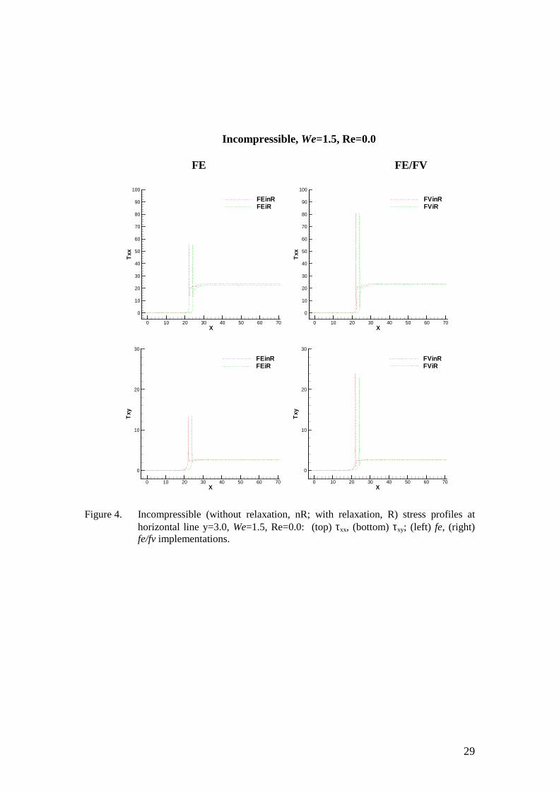
Figure 4 quantifies the above via stress profiles, for τxx (top) and τxy (bottom), at y=3.0
along the downstream boundary-wall (see Figure 2a). For plotting clarity, a shift in the
position of the re-entrant corner is introduced in under-relaxed (R)-plots. There are practically
no differences detected, with or without under-relaxation. Levels in both stress component
(τxx,τxy)-peaks at the re-entrant corner, are larger for the hybrid fe/fv above the fe-form (by
about 1.4 times for τxx and twice for τxy). One may attribute this to the deeper interpolation
quality of the hybrid form (refinement in mesh through sub-cells). Beyond the re-entrant
corner and along the wall, there is no growth of stress, reaching equitable levels
independently of the scheme employed. Scheme comparison, provides a level of confidence
in the validaty of these incompressible solutions.
Weakly-compressible liquid flow: Results are presented for both schemes in a similar
fashion to the foregoing, though field variable plots (Figure 5 as Figure 3) and stress profiles
(Figure 6 as Figure 4). Additionally, field plots are now provided for density variation (Figure
5b). Note, no under-relaxation is necessary for compressible implementations, as numerical
stability is found to be satisfactory without such measures. Oncemore, similar contour
patterns at equitable levels are observed for both schemes (discrepancy in pressure is 1%; in
density, 0.2%). Conspicuously, density representation, across the channel section
14
(x=constant), declines from the centreline to the wall, due to the relationship between density
and pressure, upheld via the Tait equation of state (Eq.(5)). In this instance, τxx (and hence
trace τ) is larger at the wall than the centreline. Note, under Newtonian conditions, density
contours mimic those in pressure.
Figure 6 illustrates solution profiles in τxx (top) and τxy (bottom), for both schemes at the
boundary wall (y=3.0). The levels of stress-peak are comparable to those of the
incompressible instance of Figure 4, when comparing both fe to fe/fv-solutions. The main
differences to observe against incompressible counterparts, lie in the sustained growth in both
stress components along the boundary wall. This growth rate is constant, described by its
angle. These angles are larger for τxx (12° for τxx compared to 4° for τxy), and reflect
independence of the specific spatial discretisation employed. At We=1.5, we notice oscillatory
patterns, behind the singularity corner, in the fe-stress plots, which disappear in the fe/fv-
profiles. This is due to the ability of the fe/fv to deal with sharp solution gradients and
superior suppression characteristics on numerical cross-stream diffusion. By design, this is
not the case with the SUPG/fe-implementation, as observed by others [37].
Scheme and flow setting comparison: Quantitative comparison of U-profiles along the
centreline (y=4, see Figure 2a) is undertaken, in Figure 7. This includes assessment of fe and
fe/fv-algorithmic implementations for both incompressible (Ma=0.0, Figure 7a) and weakly-
compressible (Ma=0.1, Figure 7b) variants. In addition, we provide Ma≈0 limit and
incompressible (Ma=0) comparison (Figure 7c, fe; Figure 7d, fe/fv). At this We-level, close
agreement is observed between implementations, under these alternative flow configurations.
The U-profile remains flat beyond the re-entrant corner plane for incompressible flow, whilst
it increases monotonically for compressible flow. This maintains a balance in mass-flow rate
( U, see Figure 7b) overall, as density at the inlet is some 30% larger than that at the exit.
Furthermore, as with stress above and for both schemes, Ma≈0 solutions lie within less than
0.1% of their incompressible equivalents.
4.4. Increasing We - solution strategy
Here, both fe and fe/fv-solutions are sought under the three Ma-flow settings for increasing
We up to critical limiting levels. Initially, liquid inertia is omitted in these calculations.
Incompressible liquid flow
In Figure 8, solution profiles for principal stress N1 are plotted across each scheme. The effect
of introducing under-relaxation (bottom) is also highlighted. We comment upon critical levels
of We attained, in passing, recorded for immediate comparison in Table 1.
15
a) Without relaxation: Stress-peaks are larger for the fe/fv-scheme (peak Wecrit=3.0)
compared to their fe-counterpart (peak Wecrit=2.2). At the same We-level, say We=2.0, there is
about 30% increase in the stress-peak for the fe/fv above the fe-form. With the fe/fv-scheme, at
We=2.0 and above, in a small region beyond the corner, the principal stress-peak is followed
by two short duration oscillations, that are rapidly damped away travelling further
downstream. Similar oscillatory behaviour has been observed earlier by both Yurun [37] and
Phillips and Williams [23].
b) With under-relaxation: At We=2.5, there is about 12% decrease in the stress-peak for
the fe/fv below the fe-variant. In contrast to the non-relaxed results at We=2.0, there is barely
any difference in stress-peak level with the fe-scheme, whilst there is about 30% reduction
with the relaxed fe/fv result. Downstream oscillations are also reduced for the relaxed fe/fv-
scheme compared to its non-relaxed form. Overall, under-relaxation enhances scheme
stability, when compared to its non-relaxed counterpart. On Wecrit-levels, with the fe-scheme,
there is increase from 2.2 to 2.8; a position matched with the fe/fv-scheme, demonstrating
increase from 3.0 to 3.5.
Weakly-compressible flow
Figure 9 illustrates corresponding N1-profiles for both Ma≈0 and Ma=0.1 settings (discarding
relaxation). Independent of flow scenario and across schemes, stress-peaks for the fe/fv-
scheme may amount to some four times larger than those of their fe-counterparts (at We=1.5,
the fe/fv-stress peak is about 40% larger for Ma≈0 and double that for Ma=0.1 compared to
their fe-counterparts). This is mainly due to sub-cell refinement and the particular reduced
corner integration technique applied: a discontinuity-capturing treatment for the corner
solution-singularity unique to the hybrid scheme [1]. When evaluating unrelaxed
compressible Ma≈0 solutions against their truly incompressible counterparts (Ma=0) for the
fe-scheme, equitable stress-levels are observed at Wecrit=1.5. This is not the case for the
corresponding fe/fv-scheme, as stress-peak levels are somewhat elevated from around 105
units for Ma=0, to 180 units for Ma≈0, see back to Figure 8. These discrepancies we would
attribute to the alternative fe/fv-discrete implementation in the corner neighbourhood (as
above); and also, to the additional sharp velocity gradient contributions made there within the
compressible formulation( )3ijTijL δ . Under the compressible configuration (Ma=0.1), the
Wecrit-level is about twice as large for the fe/fv-implementation (peak Wecrit=3.1) , when
compared to that for the fe-form (peak Wecrit=1.7). Nevertheless, when comparing
compressible, Ma≈0, Wecrit-levels against their incompressible counterparts the compressible
fe-scheme implementation reduces Wecrit (from We=2.2 to 1.5). The reverse is true for the
sub-cell fe/fv-scheme, as here the Wecrit-level actually increases (from We=3.0 to 3.3). Overall,
16
larger Wecrit-levels are achieved with the fe/fv-scheme throughout all the various flow
scenarios investigated. This is a persuasive argument to advocate the fe/fv-scheme over the
alternate fe-scheme. This elevated level of We (We=3.1) for fe/fv, in compressible
implementations, gives rise, onceagain, to post-corner oscillation, as noted above at earlier
We-levels for incompressible flow.
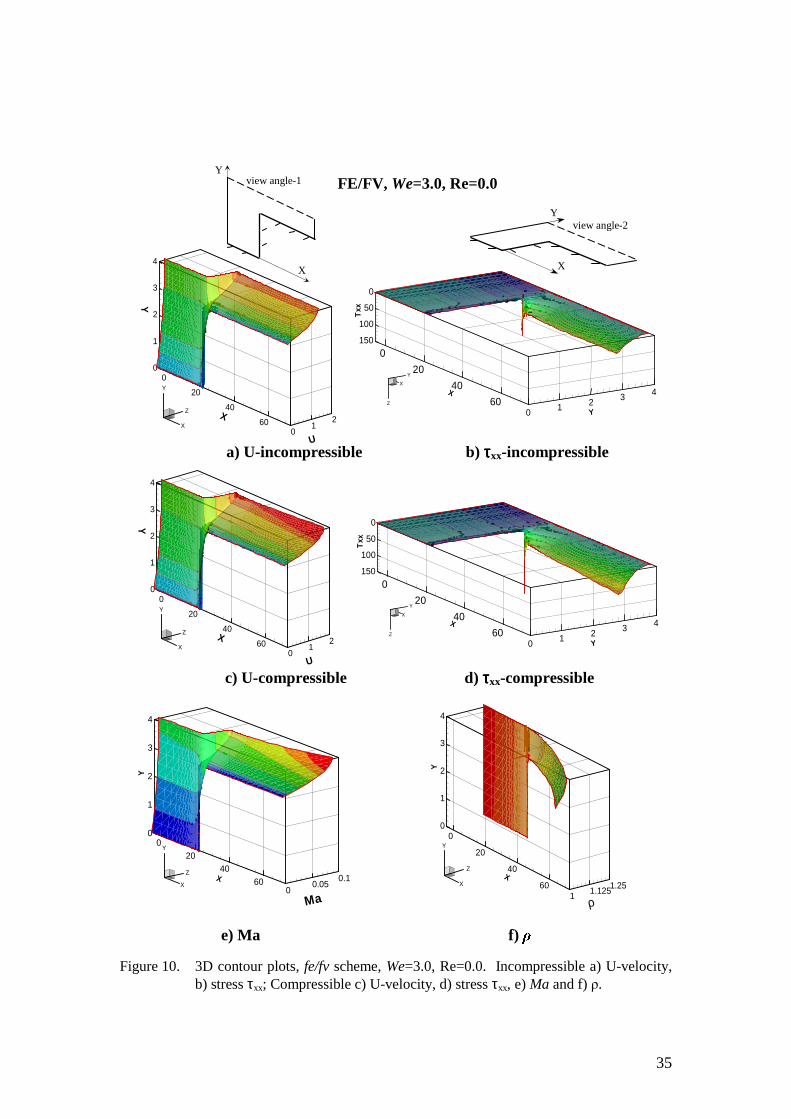
Three-dimensional field plots
Surface plots presented in Figure 10 highlight the significant differences in solutions across
the domain for the fe/fv-scheme at We=3.0. Viewing angles are displayed at the top of the
figure. This covers incompressible (Ma=0, without relaxation, the extreme level) and
compressible (Ma=0.1) flow configurations, along with variables of U-velocity (Figure 10a
and c, viewing angle-1), stress τxx (Figure 10b and d, viewing angle-2), Mach number (Figure
10e, viewing angle-1) and density (Figure 10f, viewing angle-1). In contrast to the
incompressible flow configuration, for the weakly-compressible flow, there is a sustained
increase in U-velocity along the exit-channel, corresponding to the reduction in density there
(see Figure 10f and 7b). In stress-peaks, both flows settings manifest the presence of the re-
entrant corner singularity, yet with larger peaks in the compressible over the incompressible
solutions. For the incompressible solution, beyond this position, along the exit-channel
boundary wall, there is no growth in the stress-level. In the compressible solution, the stress
sustains a monotonic growth along the wall, so that at the exit, the compressible-τxx doubles
its incompressible counterpart (see Figure 9). This may be gathered from the more excessive
cross-stream exit-flow curvature in the compressible τxx-surface plot.
Mach number contour patterns mimic those in velocity, confirming the acceleration of the
flow throughout the exit-channel. Density patterns expose the influence of stress, in relating
pressure to density. The three-dimensional surface plot at exit of Figure 10f is not straight, but
curves towards the centerline, see also Figure 5b. Correspondingly, contours are straight at
channel-entry, where density variation is negligible.
4.5. Flow patterns and vortex behaviour
In the contraction flow problem, salient-corner vortex-size and strength are major
characteristics used to quantify numerical solutions, often judged against experimental
observations. First, we summarise the position in the literature. In their experimental work,
Evans and Walters [8] reported on both lip and salient-corner vortex behaviour. They
attributed the complex characteristics encountered under vortex enhancement to several
factors: material properties, type of geometric contraction (sharp or rounded), contraction
ratio, fluid inertia and breakdown of steady flow. Prunode and Crochet [25] performed a
17
qualitative numerical comparison against these experimental results. Matallah et al., [18]
presented a comprehensive literature review on vortex activity, indicating the difficulty of
accurate prediction of lip-vortex activity. The Matallah et al., study was based on new
features in the fe-scheme, with velocity-gradient recovery applied within the constitutive
equation. There, for the creeping flow of an Oldroyd-B fluid, a lip-vortex appeared as early as
We=1.0, which grew in intensity with increasing We. This lip-vortex strength was found to be
larger than the salient-corner counterpart, from a We-level of unity and beyond. Likewise,
based on fv-discretisation, Aboubacar and Webster [1], Xue et al., [36], Oliveira and Pinho
[22], also observed the appearance of a lip-vortex at We 2.0 in [1] and We=1.6 in [36].
Oliveira and Pinho [22] claimed to detect the appearance of a lip-vortex for an UCM model at
We=1.0. Furthermore, the authors highlighted the need for a high degree of mesh refinement
required for an accurate and reliable representation of vortex activity. The influence of inertia
inclusion was also interrogated by Xue et al., [36], who concluded that although fluid inertia
had some influence on the upstream flow field, no evidence linked the appearance (or
absence) of lip-vortices with inertia. On the contrary, Phillips and Williams [23] found that
the inclusion of inertia for an Oldroyd-B model, delayed the appearance of the lip-vortex till
We=2.5 (appearing at We=2.0 for Re=0) and the salient-corner vortex-size and intensity
shrank (falling by about 20% below that for Re=0). Subsequently, Phillips and Williams [24]
observed that the size of the salient-corner vortex decayed slowly over a range, 0We 1.5,
where growth in vortex-intensity was independent of Re-level (0.0 or 1.0). Their results
agreed closely with those of Sato and Richardson [26], Matallah et al., [18] and Xue et al.,
[36]. They also recognised the sensitivity of their results to the quality of mesh employed.
Likewise, many authors have been aware of the impracticability to refine the mesh towards
the corner beyond a certain threshold, due to the consequence of approximating the
singularity. These findings demonstrate that trends in salient-corner vortex behaviour are
better characterised and predicted than is the case for lip-vortex activity. In a more recent
study, Alves et al., [4] have catalogued a set of benchmark solutions, for Oldroyd-B and PTT
models, again under planar creeping flow conditions. Solutions were produced based on a
very fine mesh of O(105) fv-cells (over one million degrees of freedom). Note here, our
present mesh has O(103) fv-cells. Oncemore, these authors demonstrated that vortex
characteristics (size and intensity) were sensitive to the particular mesh employed. On their
finest mesh, Alves et al., also observed salient-corner vortex reduction with increasing We,
and the appearance of a lip-vortex at around We=1.0 (Re=0). They found that, by
extrapolating data on lip-vortex intensity through diminishing mesh-size†, that for We=0.5 and
† Anticipating extrapolation to have some meaning, when applied to spatially shifting phenomena across meshes.
18
1.0, the lip-vortex would vanish. Yet, at We=1.5, a finite lip-vortex intensity (0.02*103) was
predicted to survive, as mesh-size tended to zero.
As above, in our current study, the focus has been on flow patterns as a function of
increasing We, emphasising steady-state salient vortex behaviour. Trends in vortex-size and
intensity for both fe and fe/fv-schemes are presented under incompressible (Ma=0, without
and with relaxation) and compressible (Ma≈0 and Ma=0.1) flow configurations. In addition,
creeping (Re=0.0) and inertial (Re=1.0) conditions are considered. Extrema (minima) in
stream-function intensity may be located either in the salient-corner vortex or lip-vortex
depending on the particular We-level. Corner-vortex cell-size, XS, is defined by convention as
the non-dimensional vortex-length from the salient-corner to the separation-streamline along
the upstream wall (see Figure 2a).
We begin with scheme and flow setting comparison for creeping flow. Under
incompressible liquid flow, we illustrate in Figure 11 (as elsewhere to follow), vortex
reduction trends in salient-corner vortex-size (top) and vortex-intensity (bottom, *10-3), under
both schemes and increasing We-level. Solutions are based on three alternative settings
(incompressible flow, both with relaxation (R) and without (nR), and compressible flow with
Ma≈0). Less than 1% difference is noted between the nR- and R-vortex-size data‡. For the
compressible implementation, Ma≈0, and in contrast to its incompressible counterpart
(Ma=0), discrepancies are uniformly around 2%.
Similarly, In Figure 12, we turn our attention to observing trends with switch in flow
setting, detecting differences under scheme variants (fe and fe/fv), for flow settings nR-
incompressible Ma=0 (left) and Ma=0.1-compressible (right). Again vortex reduction is
generally observed throughout all scenarios. Under incompressible considerations, there is
barely any difference in solutions between the two numerical schemes (differences of about
2% in intensity and less than 0.1% in size). Close agreement is found between our solutions
and those of Alves et al., [4] (included in plot) up to relatively high levels of We of 2.5. For
compressible flow conditions, fe and fe/fv-solutions differ by about 3% in size. Under any
particular We-value, compressible conditions increase vortex characteristics compared to
those for equivalent incompressible considerations (about 15% increase in size and intensity
triples). As the characteristic compressible velocity scale (defined at the outlet) is larger than
its incompressible counterpart (by about 30%, see Figure7b), this will have an effect on the
We-scale employed. To equilibrate comparison, a transformed equivalent incompressible We-
scale (We*) is also included within the compressible plots. Even on this basis, compressibility
exaggerates vortex characteristics.
‡ This rises to one order more in vortex-intensity, due to the solution size O(10-3) and the nature of this measure.
19
Streamline patterns with increasing We-level are plotted for each scheme, fe and hybrid
fe/fv, and flow conditions, incompressible and weakly-compressible. For incompressible flow,
relaxation is considered to reach elevated levels of Wecrit. In Figure 13, under the fe/fv-
scheme and creeping flow, streamlines contours are illustrated in steps of We (from 0.1 to
Wecrit) for incompressible (left) as well as compressible (right). We note, as stated above, the
larger salient-corner-vortex, as well as the lip-vortex, in the compressible flow solutions
above their incompressible counterparts. For incompressible flow solutions with the fe-
scheme (not presented here), the lip-vortex first appears beyond We=2.5 (1.9*10-4 at We=2.8).
Alternatively, under the fe/fv-variant, the lip-vortex emerges earlier at We=2.0. This was the
case in [3], there attributed to the characteristics of the hybrid scheme. In the compressible
context, a lip-vortex first appears earlier (at We=1.0). Lip-vortex intensity becomes larger, in
absolute value, for both flow configurations from the We=3.0-level onwards†. Salient-corner
vortex reduction is clearly apparent with increasing We under any flow configuration; whilst
once present, lip-vortex size grows. For compressible flow, the shape of the salient vortex
changes from its equivalent incompressible shape at We=0.1 (same in the Newtonian case) to
a more stretched, and convex form joining the lip-vortex at high We.
Inertia inclusion: With restriction to fe-solutions henceforth, Figure 14 follows Figure 12,
to demonstrate the influence of inclusion of inertia against increasing We-level. This data
address Ma≈0 (left) as well as Ma=0.1 (right) compressible flow configurations. As
anticipated, introducing inertia reduces vortex-size and intensity, a consistent trend noted
across configurations. This reduction in size for incompressible flow (Ma≈0) varies between
17% for low values of We of 0.1, to 26% over the higher range at We of 1.5 (intensities
following suit). Such trends in vortex-size are amplified for the compressible context
(Ma=0.1) to 23% at low We of 0.1, up to 36% at We=1.5.
Following Figure 14, Figure 15 charts the equivalent compressible stream-function field
solutions for inertial flow, under increasing We. The shrinkage of vortices (salient and lip) is
clearly apparent compared to those in creeping flow. For the more ubiquitous lip-vortex
activity, fe-solutions display no lip-vortex in the incompressible limit (Ma≈0), whilst one does
appear at We=1.0 in the compressible (Ma=0.1) configuration, as was the case for
compressible creeping flow. Again, at the relatively high limiting We of 2.0, lip-vortex
intensity overtakes that of the salient-corner vortex. It has already been established [9,25],
that in inertial flow there is delay in the onset of lip-vortex activity, compared to that under
creeping flow. Its absence in the incompressible instance (Ma≈0) is due to the low Wecrit (1.5)
achieved by the Ma≈0-fe-scheme (a lip-vortex appears at We=2.0 for creeping flow). Based
† For the compressible fe-scheme, not illustrated here, the lip-vortex also appears at We=1.0, with intensity of 3.7*10-4, increasing to 4.3*10-4 at Wecrit=1.7.
20
on such observations, and specifically with respect to capture of corner solution
characteristics, the sub-cell fe/fv-scheme is advocated over the parent-fe-variant.
5. Conclusions
We have investigated the abrupt four-to-one contraction benchmark problem for an Oldroyd-
B model, two numerical schemes (fe and hybrid fe/fv), and three flow settings
(incompressible-Ma=0, weakly-compressible-Ma≈0 and Ma=0.1). Solutions for both creeping
and inertial flows conditions have been presented.
For each implementation, on Wecrit and corresponding vortex activity (size and intensity),
the main differences we observe against incompressible counterparts, lie in the sustained
growth at constant rate, in both wall-stress components beyond the re-entrant corner. This is
independent of the specific spatial scheme employed. Under the incompressible context,
relaxation elevates the Wecrit-levels for both scheme implementations, as numerical stability is
enhanced. Larger Wecrit levels are reached under all three flow settings, for the fe/fv-scheme
compared to the fe-variant. This we attribute to the discretisation differences between
schemes approaching the re-entrant corner: sub-cells and use of discontinuity capturing in the
hybrid case. We note also, the property of the fe/fv-scheme to display some control on cross-
stream solution variation, particularly in the presence of sharp solution gradients. On the
vortex behaviour, at equitable We-level and flow settings, both schemes produce comparable
vortex characteristics. We observed larger salient-corner and lip-vortices in compressible flow
above its incompressible counterpart. Independently of flow setting, salient-corner vortex-size
decays with increasing We (vortex reduction), whilst lip-vortex size is enhanced. For
compressible flow, the shape of the salient vortex adopts a curved and stretched form
(separation line becomes curved), uniting with the lip-vortex at high We. Upon introducing
inertia into the problem, all aspects of vortex (salient and lip) activities are reduced
accordingly.
Further extensions to the current study shall be oriented towards seeking true transient
solutions and introducing alternative rheological models.
21
Appendix: Efficiency in computation of LMN flows
In LMN flows, the largest eigenvalue of the system (λmax) tends toward the speed of sound,
whilst the smallest (λmin) provides the speed of the fluid. The condition number of the system
( minmax / λλ=k ), goes large as the Mach number approaches zero, upholding
11 −+=+= Mau
cuk . (21)
This situation correspondingly increases the stiffness in the system [29]. Consequently, for
compressible implicit schemes, iterative solution of the algebraic equation system is slow and
expensive. On the other hand, time-marching explicit schemes suffer from excessively small
time-steps to satisfy CFL conditions. This imposes restriction on time-step selection of the
form,
cu
xatcomp +
∆≤∆ , (22)
where, a is a constant of order unity, x∆ the mesh length-scale, and (u+c) is the speed of the
acoustic mode. For the incompressible counterpart, the stability restriction is less severe:
u
xatinc
∆≤∆ , (23)
where, the time-step is in balance with the physical time-scale. One can obtain
01
→+
=∆
∆Ma
Ma
t
t
inc
comp
as 0→Ma . (24)
Thus, for LMN and explicit schemes, acoustic waves impose a much smaller time-step
than the physical time-step. Therefore, conventional compressible solvers for LMN flows,
either in explicit or implicit form, become inefficient and impractical without modification for
Ma<0.3. The problem can be quantified on the following grounds: the speed of sound for air
at room temperature is around 330 m/s. Therefore at Ma=0.3, the speed of the fluid will be
approximately 100 m/s. Nevertheless, the speed of sound for compressible liquids is much
faster than the speed of sound in air (say five times). In applications such as polymer
processing, velocity levels are generally low (of the order of unity). Therefore, system
condition numbers in compressible liquid flows are normally smaller, by an order of
magnitude, comparable to those for compressible gas dynamic applications. This is why
computation of compressible liquid flows is generally associated with much more severe
conditions than those for gas flows.
Acknowledgements: The financial support of EPSRC grant GR/R46885/01 is gratefully acknowledged.
22
References
[1] M. Aboubacar, M.F. Webster, A cell-vertex finite volume/element method on
triangles for abrupt contraction viscoelastic flows, Journal of Non-Newtonian Fluid
Mechanics 98 (2001) 83-106.
[2] M. Aboubacar, H. Matallah, M.F. Webster, Highly elastic solutions for Oldroyd-B
and Phan-Thien/Tanner fluids with a finite volume/element method: planar
contraction flows, Journal of Non-Newtonian Fluid Mechanics 103 (2002) 65-103.
[3] M. Aboubacar, H. Matallah, H.R. Tamaddon-Jahromi, M.F. Webster, Numerical
prediction of extensional flows in contraction geometries: hybrid finite
volume/element method, Journal of Non-Newtonian Fluid Mechanics 104 (2002)
125-164.
[4] M.A. Alves, P.J. Oliveira, F.T. Pinho, Benchmark solutions for the flow of Oldroyd-
B and PTT fluids in planar contractions, Journal of Non-Newtonian Fluid Mechanics
110 (2003) 45-75.
[5] P.T.F. Baaijens, Mixed finite element methods for viscoelastic flow analysis: a
review, Journal of Non-Newtonian Fluid Mechanics 79 (1998) 361-385.
[6] E.A. Brujan, A first-order model for bubble dynamics in a compressible viscoelastic
liquid, Journal of Non-Newtonian Fluid Mechanics 84 (1999) 83-103.
[7] E.O.A. Carew, P. Townsend, M.F. Webster, A Taylor-Petrov-Galerkin algorithm for
viscoelastic flow, Journal of Non-Newtonian Fluid Mechanics 50 (1993) 253-287.
[8] R.E. Evans, K. Walters, Flow characteristics associated with abrupt changes in
geometry in the case of highly elastic liquids, Journal of Non-Newtonian Fluid
Mechanics 20 (1986) 11-29.
[9] R.E. Evans, K. Walters, Further remarks on the lip-vortex mechanism of vortex
enhancement in planar-contraction flows, Journal of Non-Newtonian Fluid
Mechanics 32 (1989) 95-105.
[10] G.C. Georgiou, The time-dependent, compressible Poiseuille and extrudate-swell
flows of a Carreau fluid with slip at the wall, Journal of Non-Newtonian Fluid
Mechanics 109 (2003) 93-114.
[11] R. Guénette, M. Fortin, A new mixed finite element method for computing
viscoelastic flows, Journal of Non-Newtonian Fluid Mechanics 60 (1995) 27-52.
[12] F.H. Harlow, A. Amsden, Numerical calculation of almost incompressible flow,
Journal of Computational Physics 3 (1968) 80-93.
[13] K. Karki, S.V. Patankar, pressure based calculation procedure for viscous flows at all
speeds in arbitrary configurations, AIAA journal 27 (1989) 1167-1174.
[14] I.J. Keshtiban, F. Belblidia, M.F. Webster, Numerical simulation of compressible
viscoelastic liquids. In: Journal of Non-Newtonian Fluid Mechanics, special issue,
23
XIIIth International Workshop on Numerical Methods for non-Newtonian Flows,
Lausanne, Switzerland, 2003.
[15] R. Keunings, On the high Weissenberg number problem, Journal of Non-Newtonian
[35] J.S. Wong, D.L. Darmofal, J. Peraire, The solution of the compressible Euler
equations at low Mach numbers using a stabilized finite element algorithm, Computer
Methods in Applied Mechanics and Engineering 190 (2001) 5719-5737.
[36] S.C. Xue, N. Phan-Thien, R.I. Tanner, Three dimensional numerical simulations of
viscoelastic flows through planar contractions, Journal of Non-Newtonian Fluid
Mechanics 74 (1998) 195-245.
[37] F. Yurun, A comparative study of the discontinuous Galerkin and continuous SUPG
finite element methods for computation of viscoelastic flows, Computer Methods in
Applied Mechanics and Engineering 141 (1997) 47-65.
25
List of Figures
Table 1. Critical We level for different scheme variants and flow configurations. Figure 1. Hybrid fe/fv spatial discretization, a) schematic diagram of fe-cell with 4 fv sub-cells, b)
LDB-scheme, defining angles in fv-cell, c) MDC area for node l. Figure 2. a) Contraction flow schema, b) Mesh around the contraction
Figure 3. Incompressible field contours, We=1.5, Re=0.0: a) P, b) τxx, c) τxy, d) Ψ ; (left) fe, (right) fe/fv implementations.
Figure 4. Incompressible (without relaxation, nR; with relaxation, R) stress profiles at horizontal
Figure 5. Compressible (Ma=0.1) field contours, We=1.5, Re=0.0: a) P, b) ρ , c) τxx, d) τxy, e) Ψ ;
(left) fe, (right) fe/fv implementations. Figure 6. Compressible (Ma=0.1) stress profiles at horizontal line y=3.0, We=1.5, Re=0.0: (top)
τxx, (bottom) τxy; (left) fe, (right) fe/fv implementations. Figure 7. U-velocity profiles at centreline, We=1.5, Re=0.0: (top) fe vs. fe/fv: a) incompressible, b)
compressible; (bottom) incompressible vs. Ma≈0 limit: c) fe, d) fe/fv implementations. Figure 8. N1-profiles at horizontal line y=3.0 increasing We, Re=0.0. Incompressible: (left) fe and
(right) fe/fv implementations; (top) without relaxation, (bottom) with relaxation. Figure 9. N1-profiles at horizontal line y=3.0, increasing We, Re=0.0. Compressible: (left) fe and
Ma≈0 (left) and Ma=0.1 (right); creeping vs. inertial flow.
Figure 15. Streamline contours, increasing We: (left) incompressible and (right) compressible; inertial flows, fe scheme, vortex intensity*10-3.
26
Figure 1. Hybrid fe/fv spatial discretization, a) schematic diagram of fe-cell with 4 fv sub-cells, b) LDB-scheme, defining angles in fv cell, c) MDC area for node l.
l Tc)
k
γ1
i
j
γ2
0 a
b)
a)
i
k j
27
a)
b)
Figure 2. a) Contraction flow schema, b) Mesh around the contraction
7.5
27.5
76.5
1
U =V =0
U=0, τ xy=0
P=0, U (by B.I.), V=0
U =V =0
4
y x
U , τxx,
τxy
Waters & King V =0 =τ
yy
XS
M3
28
Figure 3. Incompressible field contours, We=1.5, Re=0.0: a) P, b) τxx, c) τxy, d) ; (left) fe,