Computational approach to quantum encoder design for purity optimization
Naoki Yamamoto*Department of Engineering, Australian National University, Canberra, Australian Capital Territory 0200, Australia
Maryam Fazel†
Control and Dynamical Systems, California Institute of Technology, Pasadena, California 91125, USA�Received 28 August 2006; revised manuscript received 7 May 2007; published 26 July 2007�
In this paper, we address the problem of designing a quantum encoder that maximizes the minimum outputpurity of a given decohering channel, where the minimum is taken over all possible pure inputs. This problemis cast as a max-min optimization problem with a rank constraint on an appropriately defined matrix variable.The problem is computationally very hard because it is nonconvex with respect to both the objective function�output purity� and the rank constraint. Despite this difficulty, we provide a tractable computational algorithmthat produces the exact optimal solution for codespace of dimension 2. Moreover, this algorithm is easilyextended to cover the general class of codespaces, in which case the solution is suboptimal in the sense that thesuboptimized output purity serves as a lower bound of the exact optimal purity. The algorithm consists of asequence of semidefinite programmings and can be performed easily. Two typical quantum error channels areinvestigated to illustrate the effectiveness of our method.
The efficient transmission of quantum states over a noisychannel is a central subject in quantum-information tech-nologies �1�. The mathematical description of a quantuminput-output relation is as follows. Let H and K be finite-dimensional Hilbert spaces of an input quantum state and thecorresponding output, respectively. We denote by L�H ,K�the set of linear operators from H to K, and S�H� the set ofquantum states on H. The Markovian evolution of a quantumstate ��S�H� through a quantum channel A is typicallymodeled using the Kraus representation �2� as
�� = A� = �i
Ai�Ai†, �1�
where the Kraus operators Ai�L�H ,K� satisfy �iAi†Ai= IH
with IH denoting the identity operator on H. The purity of astate � is defined as p���ªTr��2�, which is equal to 1 if andonly if � is pure. Due to the decoherence caused by A, a pureinput state �= ������ may be transmitted to a nonpure output��=A�������� with p�����1. It is considered that p����quantifies an intrinsic measure of the amount of decoherenceinduced by the error channel A. In particular, this paper fo-cuses on the optimal purity
P�A� ª maxC�H
min��c��C
Tr�A���c���c��2� , �2�
where the minimization with respect to the state ��c� takesinto account the worst-case scenario of information process-ing. The maximization with respect to the codespace C�His motivated by the fact that we often have an opportunity todecrease the effect of decoherence by encoding our informa-tion into a higher-dimensional space; this is suggested by the
theories of quantum error correction �1,3–5� anddecoherence-free subspace �DFS� �6–8�. For example, em-bedding an input state ���=�1�0�+�2�1��C2 into acodespace spanned by �00� and �11� through the encodingprocess
C2 � ��� → ��c� = �1�00� + �2�11� � C � H = C4 �3�
appears to improve the output purity. Clearly, the most desir-able situation is the existence of a DFS, i.e., a codespace thatsatisfies P�A�=1; but unfortunately this is a rare case. In thissense, the optimal codespace C is regarded as the best pos-sible approximation of a DFS.
However, the max-min problem �2� is very hard to solvebecause it is nonconvex with respect to both C and ��c�. Tounderstand the structure of P�A�, in �9� Zanardi and Lidarconsidered channel purity for a fixed codespace C as
P�A,C� ª min��c��C
Tr�A���c���c��2� , �4�
and derived the alternative expression
P�A,C� = min��c��C
��c� � ��c���A���c� � ��c� ,
where the Hermitian operator ��A� is defined by
��A� ª �ij
�Aj†Ai� � �Ai
†Aj� � L�H�2,H�2� . �5�
This expression was used to derive a bound on P�A ,C� interms of ��A� and C, using techniques to calculate the ex-pectation value of the “Hamiltonian� ��A�. In the specialcase where eigenvectors of ��A� are product states in a sym-metric subspace of H�2, analytical expressions for P�A ,C�were obtained. However, in general the max-min problem �2�does not have an analytical solution, leading us to take acomputational approach.
From a computational point of view, owing to the rapidprogress of computers, there have been many recent ad-
vances with a great potential for solving important problemsin quantum theory. Convex optimization, and in particularsemidefinite programming �SDP� �10,11�, have proven usefulfor quantum optimization problems such as a test for distin-guishing an entangled from a separable quantum state�12–16� and a design of optimal measurement in linear quan-tum systems �17�. In addition, in �18–20� some quantumerror-correction problems were solved using SDP, taking ad-vantage of the well-known convexity of a set of quantumchannels known as the Jamiolkowski isomorphism �21�.
In this paper, we first use the same convexity property toset up a nonconvex optimization problem that captures ourgoal and all the constraints. Then, we provide an algorithmthat computes an exact local optimal solution of the hardnonconvex problem �2� for the codespace of dim C=2. Thisimplies that the exact global optimal solution of �2� can beobtained by appropriately choosing an initial condition of thealgorithm. The algorithm is represented by an iterative SDPand is thus computationally tractable. The derivation of theSDP consists of two stages. The first one transforms the con-straints to equivalent linear matrix inequality �LMI� con-straints. The key idea used to obtain the LMI in this stage isthe sum-of-squares characterization of a polynomial con-straint �22–24�. In the second stage, a nonconvex rank con-straint of the matrix variable is tackled via the log det �loga-rithm of determinant� heuristic �25–27�. Furthermore, wewill show an extended version of the above SDP algorithmthat computes a lower bound of the optimal purity P�A� forthe general class of C.
This paper is organized as follows. Section II reviews theJamiolkowski isomorphism, which is used to formulate theoptimization problem in Sec. III. The SDP algorithm is pre-sented in Sec. IV. The general case that leads to a suboptimalsolution is discussed in Sec. V. In Sec. VI, we examine twotypical quantum error channels, the bit-flip channel and theamplitude damping channel, and demonstrate the effective-ness of our method. Section VII concludes the paper.
Notation. A Hermitian matrix X=X†�L�Cn ,Cn� is posi-tive semidefinite if �a�X�a��0, ∀ �a��Cn; the inequality X�0 represents the positive semidefiniteness of X. We use Into denote the n�n identity matrix, which is the same as IHwhen dim H=n. For a matrix X= �xij�, the symbols XT andX* represent the matrix transpose and the elementwise com-plex conjugate of X, i.e., XT= �xji� and X*= �xij
* �= �X†�T, re-spectively; these rules are applied to any rectangular matrixincluding column and row vectors. Re�X� and Im�X� denotethe real and imaginary parts of X, respectively, i.e.,�Re�X��ij = �xij +xij
* � /2 and �Im�X��ij = �xij −xij* � /2i.
II. THE JAMIOLKOWSKI ISOMORPHISM
The main purpose of this section is to review the follow-ing important fact known as the Jamiolkowski isomorphism�21�: the set of all finite-dimensional quantum channels has aone-to-one correspondence with a convex set of positivesemidefinite matrices acting on K � H. This fact can be seenin various ways �18,28–30�. Here we follow the notations in�18,30� and obtain two matrix representations of a quantumchannel, which we later use to set up the optimization prob-
lem. At the end of this section, we present a characterizationof quantum channels that preserve pure states.
We consider a general trace-preserving quantum channelthat maps an input ��S�H�=S�Cn� to the output
�� = �i
Xi�Xi† � S�K� = S�Cm� . �6�
Let �i�i=1,. . .,n and �i�i=1,. . .,m be orthonormal bases in H andK, respectively. Then, any vectors in H�2 and K�2 are ex-
pressed as ����=�i,j=1n �ij�i� � �j� and �����=�i,j=1
m �ij� �i� � � j�,respectively. We sometimes use �i��j� as a shorthand for �i�� �j�. Let us now define the following two specific vectors:
�IH�� ª �i=1
n
�i� � �i�* � H�2, �7�
�IK�� ª �i=1
m
�i� � �i�* � K�2. �8�
These vectors have the property of being independent of theselection of orthonormal basis; for any two orthonormalbases �ai� and �bi� in H, we have
�IH�� = �i=1
n
�ai� � �ai�* = �i=1
n
�bi� � �bi�*. �9�
Note that the invariant property �9� is not satisfied if �IH�� isdefined without the complex conjugation. The vectors �7�and �8� are related by
�X � IH��IH�� = �IK � XT��IK��, ∀ X � L�H,K� .
�10�
Further, the following equation holds:
��IH��X � IH��IH�� = TrX, ∀ X � L�H,H� . �11�
We now define a positive semidefinite matrix X1 associatedwith the Kraus operators Xi�L�H ,K� as
X1 ª �i
�Xi � IH��IH����IH��Xi � IH�† � L�K � H,K � H� .
Then, the trace-preserving condition �iXi†Xi= IH corresponds
to TrKX1= IH, and the quantum channel �6� is expressed interms of X1 as
�� = TrH��IK � �T�X1� . �12�
Conversely, it is known that any positive semidefinite matrixX1�L�K � H ,K � H� corresponds to a quantum channelwith input-output relation given in Eq. �12�. That is, thereexists a one-to-one correspondence between a quantum chan-nel from H to K and a positive semidefinite matrix on K� H.
We next introduce another matrix representation of thequantum channel, which will be denoted by X2. To this end,we define a vector associated with a quantum state ��S�H� as
NAOKI YAMAMOTO AND MARYAM FAZEL PHYSICAL REVIEW A 76, 012327 �2007�
012327-2
���� ª �� � IH��IH�� � H�2. �13�
The vector ���� is obviously in one-to-one correspondencewith �. In particular, from Eq. �9�, the vector representationof a pure state �= �a��a� is given by
���� = ��a��a� � IH��i
�i� � �i�* = �a� � �a�*. �14�
In addition, the purity p���=Tr��2� is simply the squaredEuclidean norm of ����:
p��� = Tr��2� = ������� , �15�
due to Eq. �11�. Thus, a quantum state ���� is pure if and onlyif ��� ����=1. Let us now define X2. Multiplying �IK�� on bothsides of Eq. �6�, we have ��� � IK��IK��=�i�Xi�Xi
†� IK��IK��,
which is rewritten as
��� � IK��IK�� = �i
�Xi � IK��� � IK��IH � Xi*��IH��
= �i
�Xi � Xi*��� � IH��IH�� ,
because of the property �10�. Hence, defining the matrix
X2 ª �i
Xi � Xi* � L�H�2,K�2� ,
the quantum channel �6� is represented by
H�2 � ���� → ����� = X2���� � K�2.
The trace-preserving condition is then given by
��IK�X2 = �i
��IK��Xi � IK��IH � Xi*�
= �i
��IH��IH � XiT��IH � Xi
*� = ��IH� .
The matrix X2 is related to X1 through the following rear-rangement rule of the matrix elements:
�i�� j�*X2�k����* = �i��k�*X1� j����*.
This relation is independent of the selection of �i� and �i�due to Eq. �9�. As the rearrangement map is obviously linearand homeomorphic, X1 and X2 have a one-to-one correspon-dence with each other. We denote this relation by X1=��X2�. The above discussion is summarized as follows.
Lemma 1. Any finite-dimensional quantum channel fromH to K is represented by H�2� ����→ �����=X�����K�2,where X is in the set
The linear transformation ��X� is defined with respect to
orthonormal bases �i��H and �i��K as
�i�� j�*X�k����* = �i��k�*��X�� j����*.
Clearly, X�H ,K� is a convex set with dimension m2n2
−n2. It should be noted that a cascade connection of twoquantum channels X�X�H ,K� and X�X�K ,V� is simply
represented by the multiplication of those matrices: YX�X�H ,V�.
Finally, we provide a characterization of quantum chan-nels that preserve pure states, i.e., p���= p����=1, as follows.
Lemma 2. For a quantum channel X�X�H ,K�, the fol-lowing three conditions are equivalent:
�i� X�a�� is pure for any pure state �a��= �a� � �a�*.�ii� X†X= IH�2 = In2.�iii� rank ��X�=1.Proof. �i� ⇔ �ii�. Condition �ii� immediately implies that
�a���=X�a�� is pure, since p�a��= ��a��a���= ��a�X†X�a��= ��a �a��=1. Conversely, as X can be represented by X=�i=1
M Xi � Xi*, the quantum state �a���=X�a�� always satisfies
the following relation:
��a��a��� = ��a�X†X�a��
= �a��a�*�i,j
�Xi†
� XiT��Xj � Xj
*��a��a�*
= �i,j
��a�Xi†Xj�a��2 � �
i,j�a�Xi
†Xi�a��a�Xj†Xj�a� = 1.
�16�
Therefore, the condition ��a� �a���=1 imposes the equalityrelation in Eq. �16�. Then, Xi�a� is parallel to Xj�a� for all�i , j� and �a�, indicating that Xi is independent of i. Thus, Xtakes the form X=X � X*, where X is defined by Xª
�MXi.Consequently, using the trace-preserving condition X†X= IH,we arrive at X†X= In2.
�ii�⇔ �iii�. First, we assume �iii�. Then, ��X� is written as��X�= �x����x� using a vector �x���K � H. Furthermore, as�x�� can be represented by �x��= �X � IH��IH�� with a matrixX�L�H � K�, we have ��X�= �X � IH��IH����IH��X � IH�†,and thus X=X � X* from the definition of �. This directlyyields X†X= In2 due to X†X= IH. We next turn to the proof of�ii�⇒ �iii�. Multiplying a pure state �a��= �a� � �a�*�H�2 onboth sides of In2 =X†X where X=�iXi � Xi
*, we obtain
1 = ��a�a�� = ��a�X†X�a��
= �i,j
��a�Xi†Xj�a��2
� �i,j
�a�Xi†Xi�a��a�Xj
†Xj�a� = 1.
Hence, from the same reason as in the proof of �i�⇒ �ii�, Xmust be of the form X=X � X*. This implies ��X�= �X � IH��IH����IH��X � IH�† and thus rank��X�=1. �
Corollary 1. Suppose X�X�H ,K� satisfies rank��X�=1.Then, the nonzero eigenvalue of ��X� is given by n=dimH.
Proof. From the proof of Lemma 2, we have
Tr��X� = ��IH��X†X � IH��IH�� = ��IH�IH�� = n . �
According to Lemma 2, the totality of quantum channelsthat transform pure states in H to pure in K is completelycharacterized by the following nonconvex set:
COMPUTATIONAL APPROACH TO QUANTUM ENCODER… PHYSICAL REVIEW A 76, 012327 �2007�
012327-3
X1�H,K� = X � L�H�2,K�2� � rank ��X� = 1,
��X� � 0, ��IK�X = ��IH� .
III. OPTIMAL ENCODER DESIGN AS A MATRIX-OPTIMIZATION PROBLEM
This section is devoted to rewriting the problem �2� as anencoder-optimization problem, which is further described asa matrix-optimization problem using the notations intro-duced in Sec. II.
First, let us fix the dimension of the codespace C todim C=r and represent an element of C by ��c�=E��� withthe input pure state ����Cr which contains all informationof the sender. Here, E is the Kraus operator corresponding tothe following encoding channel:
E : Cr � ��� → ��c� = E��� � C � H . �17�
We set H=Cn; then, E is an n�r complex matrix satisfyingE†E= Ir. In the example �3�, ��� is a qubit and E= �00��0�+ �11��1�, i.e., r=2 and n=4. In terms of the above notations,the codespace-optimization problem �2� is written as
Next, let us represent the problem using the matrix vari-able introduced in Sec. II. Since the encoding channel E ob-viously preserves pure states, its matrix representation E isan element of X1�Cr ,Cn�. Also, from Eq. �14�, the input ���takes the form ����= ��� � ���* in the extended space �Cr��2.Hence, the output state of the encoder-error process is givenby �����=AE������*, where A�X�Cn ,Cn� is the matrix rep-resentation of the error channel A. Then, due to Eq. �15�, theoutput purity is
P�A,E, ���� = ��������� = ������*E†A†AE������*.
Consequently, the max-min problem �18� is written as
P�A� = maxE�X1
min����Cr
������*E†A†AE������*, �19�
which is identical to the following “error-minimization”problem:
minE,
,
such that ������*E†A†AE������* � 1 − , ∀ ��� � Cr,
E � X1�Cr,Cn� ,
0 � � 1. �20�
Note that the optimal purity is related to the minimum erroropt by
P�A� = 1 − opt.
IV. EXACT OPTIMAL SOLUTION TO THE PURITY-OPTIMIZATION PROBLEM
In this section, we provide a systematic and powerfulcomputational algorithm that exactly solves the purity-optimization problem when dim C=r=2. The proposed algo-rithm can easily be extended to cover the general class ofcodespaces of dimension r�3, in which case the subopti-mized output purity gives a lower bound of the optimal pu-rity P�A�. This result will be discussed in Sec. V.
The procedure to derive the algorithm consists of twostages. In the first stage, it will be proved that the first con-straint in the problem �20�,
������*E†A†AE������* � 1 − , ∀ ��� � C2, �21�
can be equivalently transformed to a LMI condition withrespect to E ,, and an additional variable. In the secondstage, we will consider a tractable rank-minimization prob-lem of the matrix variable that is closely related to the origi-nal error-minimization problem �20�. It will be then shownthat, under a certain condition, the optimal solution of therank-minimization problem coincides with that of the prob-lem �20�.
A. The first stage: Transformation of the constraint
To simplify the exposition, we here assume that the inputstate ��� is a real-valued qubit, i.e., ���= �x1 ,x2�T�R2, �x1
2
+x22=1�. The general qubit case ����C2 will be discussed in
Sec. IV C using essentially the same idea presented here.Before considering the transformation of the constraint
�21�, let us further express it only in terms of real matrices.To this end, we define the following real matrix variable withthe size 2n2�4:
E ª Re�E�Im�E� � . �22�
Then the output purity is expressed as
P�A,E, ���� = ������ETPE������ ,
where P is a real positive semidefinite matrix defined by
P ª Re�A†A� − Im�A†A�Im�A†A� Re�A†A� � .
Furthermore, we introduce a matrix �31�
NAOKI YAMAMOTO AND MARYAM FAZEL PHYSICAL REVIEW A 76, 012327 �2007�
012327-4
B ª �1 0 0
0 1/�2 0
0 1/�2 0
0 0 1� �23�
and define a vector
�x��B ª BT������ = BT x1
x2� � x1
x2� = � x1
2
�2x1x2
x22 � .
Note that �x��B is normalized: B��x �x��B=1. As a result, fromthe relation ������=B�x��B, the constraint �21� is expressedas
We are now in a position to describe the transformation.The constraint �24� indicates that p�x� must be a real fourth-order non-negative polynomial function with respect to thevariables �x1 ,x2�. This type of constraint, i.e., the non-negativity of a polynomial function, frequently appears in awide variety of engineering problems. In particular, the fol-lowing sum-of-squares �SOS� characterization of non-negative polynomials, first studied by Hilbert more than acentury ago, is a fundamental question: When does a non-negative polynomial p�x� have a SOS decomposition p�x�=�ihi
2�x� for some polynomials hi�x�? One of the well-known answers to the above question leads us to concludethat the nonnegative polynomial p�x� must have a SOS de-composition, thereby Eq. �24� is equivalently replaced by thefollowing matrix inequality:
BTETPEB + � − 1�I3 + S + T1TETPET2 + T2
TETPET1
− T3TETPET4 − T4
TETPET3 � 0, �25�
where �R is an additional optimization variable. The proofof Eq. �25� and the matrices T1 ,T2 ,T3 ,T4, and S are given inAppendix A. The inequality �25� is transformed to
S + � − 1�I3 − �EB
ET1
ET2
ET3
ET4
�T
�kI2n2 − P
kI2n2 − P
− P kI2n2
kI2n2 P
P kI2n2
��EB
ET1
ET2
ET3
ET4
�+ k�BTETEB + T1
TETET1 + T2TETET2 + T3
TETET3 + T4TETET4� � 0, �26�
where the blank spaces in the large matrix denote zero en-tries. The fixed scalar number k�0 is selected such that
kI2n2 − P � 0 �27�
is satisfied. This is equivalent to
kI2n2 P
P kI2n2� � 0, kI2n2 − P
− P kI2n2� � 0. �28�
Then, due to the conditions �27� and �28�, the large matrix inEq. �26� is positive definite. Moreover, we now see from
Lemma 2 that the nonconvex rank condition rank��E�=1 isequivalent to E†E= I4, which leads to
ETE = Re�E�TRe�E� + Im�E�TIm�E� = I4.
Thus, the last term in Eq. �26� is calculated as
BTB + T1TT1 + T2
TT2 + T3TT3 + T4
TT4 = 2I3.
Finally, the Schur complement �see Appendix B� is used totransform Eq. �26� to
0
Xi
opt : global minimum
local minimum
X
X
FIG. 1. The log-det function and a convergence of the iterationvariable Xi.
COMPUTATIONAL APPROACH TO QUANTUM ENCODER… PHYSICAL REVIEW A 76, 012327 �2007�
012327-5
��kI2n2 − P�−1
EB
kI2n2 − P
− P kI2n2�−1 ET1
ET2
� kI2n2 P
P kI2n2�−1 ET3
ET4
�BTET �T1
TET T2TET� �T3
TET T4TET� S + �2k + − 1�I3
� � 0, �29�
which is obviously a LMI with respect to the variables E, ,and . As a result, the original problem is equivalently writ-ten by
The tuning parameter ��0 gives the relative weight be-tween the two objectives rank��E� and . This change of theproblem is motivated by the fact that we can now apply someknown heuristic methods for rank-minimization problems,one of which is discussed below.
The minimization of the rank of a matrix subject to con-vex constraints is a ubiquitous problem in diverse areas ofengineering such as control theory, system identification, sta-tistics, signal processing, and computational geometry �26�.The general rank-minimization problem
min rank X such that X � M and X � 0,
where X�0 is the optimization matrix variable and M is aconvex set denoting the constraints, is computationally NPhard; thus we need to rely on heuristics. The log det heuristicintroduced and discussed in �25–27� provides an attractiveapproach. The heuristic is described as follows. The function
log det�X+ I� is used as a smooth surrogate for rankX toyield
min log det�X + I� such that X � M and X � 0,
where �0 is a small regularization constant, and can bechosen to be on the order of the eigenvalues we can consideras zero. Although the surrogate function log det�X+ I� is notconvex, it is smooth on the positive definite cone and can beminimized locally using any local minimization method; wehere use iterative linearization. Let Xi denote the ith iterate ofthe optimization variable X. The linearization of log det�X+ I� around Xi is given by
where we have used the fact that � log det X=X−1 when X�0. Hence, we can minimize log det�X+ I� over the con-straint set M by iteratively minimizing the local lineariza-tion �34�. This leads to
Xi+1 = arg minX�M
Tr��Xi + I�−1X� .
The new optimal point is Xi+1. Since the log det function isconcave in X, at each iteration its value decreases, and thesequence of the function values generated converges to alocal minimum of log det�X+ I�. This implies that the globaloptimal solution Xopt can be obtained by appropriately choos-ing an initial point X0 �see Fig. 1�.
The above procedure is directly applicable to the casewhere the objective function is replaced by rankX+� with� �0,1� an additional variable and ��0 a constant. There-fore, the rank-minimization problem �32� is replaced by
minE,,
log det���E� + I2n� + � ,
such that �E,,� � N . �35�
The local or global optimal solution of this problem is ob-tained by solving the following iterative SDP:
�Ei+1,i+1,i+1� = min arg�E,,��N
„Tr���Ei� + I2n�−1��E� + �… .
�36�
Note that the convergence point of this algorithm is verysensitive to an initial point E0. �We do not need to specify 0
NAOKI YAMAMOTO AND MARYAM FAZEL PHYSICAL REVIEW A 76, 012327 �2007�
012327-6
and 0, since i and i are not used to calculate�Ei+1 ,i+1 ,i+1�.�
We now provide an important theorem that connects thereplaced problem �35� with the original problem �30�.
Theorem 1. If the local �global� optimal solution�Eopt ,opt ,opt� of the problem �35� satisfies rank��Eopt�=1,then it coincides with the local �global� optimal solution ofthe problem �30�.
Proof. The global optimal solution of �35� satisfies
for all �E , ,��N. From the assumption and Corollary 1,the nonzero eigenvalue of ��Eopt� is dim Cr=2, which yieldsdet���Eopt�+ I2n�= �2+ � 2n−1. Also, any E�X1�C2 ,Cn�satisfies det���E�+ I2n�= �2+ � 2n−1. As a result, Eq. �37�reduces to
opt � , ∀ �E,,� � N1,
where N1 is defined in Eq. �31�. This implies that�Eopt ,opt ,opt� is indeed the global optimal solution of �30�.We can prove the same fact for any local optimal solution byconsidering local regions of N and N1. �
Clearly, the above theorem can be extended to the generalcase of r. Therefore, the optimal �suboptimal� solution of theoriginal problem �20� is obtained by equivalently transform-ing �relaxing� it to a problem of the form �30� and solving arelated rank-minimization problem via the same heuristic.
Finally, let us discuss choosing an initial point E0 of thealgorithm �36� such that the iteration variable �Ei ,i ,i� con-verges to a local optimal solution �EN ,N ,N� withrank��EN�=1. We here make the following observation: aninitial point E0 that also satisfies rank��E0�=1 might be agood candidate for the above requirement to be satisfied.From the proof of Lemma 2, this implies
E0 = E0 � E0*, E0
†E0 = I2. �38�
Actually, in many practical cases, we observe that an initialpoint of the form �38� converges to a feasible local optimalsolution. This fact will be seen in Sec. VI.
C. Exact optimal encoder for general qubit inputs
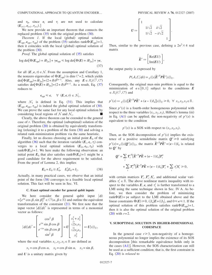
We here consider the general qubit input ���= �ei� cos � , sin ��T�C2�� ,��R� and outline the equivalenttransformation of the constraint �21�. We first note that theinput vector ������* is represented in terms of a monomialvector as follows:
������* = �cos2 �
ei� sin � cos �
e−i� sin � cos �
sin2 �� = U�
x12 + x2
2
�2x1x3
�2x2x3
x32
�¬ U�x��U,
where the real variables x1 ,x2 ,x3�R are defined as
x1 = cos � cos �, x2 = cos � sin �, x3 = sin � ,
and U is a unitary matrix given by
U ª �1
1/�2 i/�2
1/�2 − i/�2
1� .
Then, similar to the previous case, defining a 2n2�4 realmatrix
E� ª Re�EU�Im�EU� � ,
the output purity is expressed by
P�A,E, ���� = U��x�E�TPE��x��U.
Consequently, the original max-min problem is equal to theminimization of � �0,1� subject to the conditions E�X1�C2 ,Cn� and
Since p��x� is a fourth-order homogeneous polynomial withrespect to the three variables �x1 ,x2 ,x3�, Hilbert’s lemma �iii�in Eq. �A1� can be applied; the non-negativity of p��x� isequivalent to the condition
p��x� is a SOS with respect to �x1,x2,x3� .
Then, as the SOS decomposition of p��x� implies the exis-tence of a positive semidefinite matrix Q��0 satisfying
p��x�= U��x�Q��x��U, the matrix E�TPE�+ �−1�I4 is relatedto Q� by
Q� = �i
Ti�T�E�TPE + � − 1�I4�Ti�
+ �i
Ti�T�E�TPE + � − 1�I4�Ti� + �
i
i�Si� � 0,
with certain matrices Ti� ,Ti� ,Si�, and additional scalar vari-ables i��R. The above nonlinear matrix inequality with re-spect to the variables E ,, and i� is further transformed to aLMI using the same technique shown in Sec. IV A. As be-fore, we then consider the problem of minimizingrank��E�+� subject to the LMI obtained above and thelinear constraints ��E��0, ��In�E= ��I2�, and 0��1. If theoptimal solution of this problem satisfies rank��Eopt�=1,then it is also the optimal solution of the original problem�20� with r=2.
V. SUBOPTIMAL SOLUTION IN HIGHER-DIMENSIONALCODESPACE
In the general case r�3, non-negativity of a homoge-neous polynomial no longer implies the existence of its SOSdecomposition �this remarkable equivalence holds only inthe cases �A1��. However, the SOS characterization can stillbe used as a sufficient condition; that is, the first constraint inEq. �20� is relaxed to
COMPUTATIONAL APPROACH TO QUANTUM ENCODER… PHYSICAL REVIEW A 76, 012327 �2007�
012327-7
p��x� ª ��x��E�TPE� + � − 1�Ir2��x��
is an SOS with respect to �x1, . . . ,x2r−1� , �39�
where E��R2n2�r2is an appropriately defined real matrix
variable that is linear to E, and �x���Rr2is an appropriately
defined real monomial vector of x1 , . . . ,x2r−1. The SOS con-dition �39� equivalently leads to a LMI as seen before, andconsequently we have a problem of the form �30� that can betackled via the log det heuristic. Note again that Eq. �39� isonly a sufficient condition for the inequality p��x��0 to besatisfied for all �x1 , . . . ,x2r−1�. Thus, any feasible solution
�E� ,� satisfying Eq. �39� is included in the original set ofsolutions. Therefore, the suboptimal error computed from therelaxed problem, sub, is always bigger than or equal to theexact optimal error opt. This indicates that the suboptimaloutput purity, Psub�A�=1−sub, gives a lower bound of theoptimal purity:
P�A� = 1 − opt � 1 − sub = Psub�A� .
An important fact to be noticed is that, as pointed out in �24�,the gap between the set of non-negative polynomials and theset of polynomials with a SOS decomposition is consideredto be small in a practical situation. Hence, we expect thatPsub�A� is a good approximation to P�A�.
VI. EXAMPLES
A. The bit-flip channel
The quantum bit-flip channel with flipping probability p isgiven by
S�C2� � � → T1� = p�x��x + q� � S�C2� ,
where p+q=1 and �x= �0��1�+ �1��0�. We here consider thedouble bit-flip channel Abf=T1
�2:
S�C4� � � → �� = Abf� = �i=1
4
Ai�Ai† � S�C4� ,
A1 = p�x � �x, A2 = �pq�x � I2,
A3 = �pqI2 � �x, A4 = qI2 � I2.
The matrix form of the double bit-flip channel, Abf=�iAi� Ai
*�X�C4 ,C4�, is represented by
Abf = �qA4 �pqA3
�pqA2 pA1
�pqA3 qA4 pA1 �pqA2
�pqA2 pA1 qA4 �pqA3
pA1 �pqA2�pqA3 qA4
� .
In particular, we set p=0.1; then, for example, k=2 satisfiesthe condition �27�: kI32−P�0.
We here assume that the input is a real-valued qubit: ����R2. Then, an exact local or global optimal encoder Eopt�X1�R2 ,C4� is computed by the algorithm �36� under the
condition rank��Eopt�=1. A strong convergence property ofEi is observed when the SDP parameters are set to =0.01and �=15. We usually need 90 iterations of the SDP; hencewe denote the convergence point by �E90,90,90�. Noteagain that E90 must be of the form E90=E90 � E90
* due to therank condition rank��E90�=1. Regarding the initial point E0,we follow the idea mentioned in the last paragraph of Sec.IV B and examine some initial points of the form �38� to findthe global optimal solution.
First, we randomly choose two initial points as E0�j�=E0
�j�
� E0�j�*�j=1,2�, where the Kraus operators E0
�1� and E0�2� are
given by
E0�1� =
1�10�
2 0
�2 − �6
�3 1
1 �3�, E0
�2� =1
�10��2 0
�3 − �6
1 �2
2 �2� ,
respectively. Then, the corresponding convergence points arerespectively given by E90
�j�=E90�j�
� E90�j�* �j=1,2�, where
E90�1�,E90
�2�
= ��0.5308 − 0.4672
0.5308 − 0.4672
0.4672 0.5308
0.4672 0.5308�, �
0.5274 − 0.4710
0.5274 − 0.4710
0.4710 0.5274
0.4710 0.5274�� .
In both cases, the convergence value of the error is given by90=0.18. In view of the structure of E90
�1� and E90�2�, we expect
that the encoder E�a�:
E�a� = E�a�� E�a�*, E�a� =
1�2�
cos � − sin �
cos � − sin �
sin � cos �
sin � cos �� �40�
will be a local optimal solution and provide a local minimumof the error, �a�=0.18, for all �� �0,2��. In fact, for theinput ���= �x1 ,x2�T= �cos � , sin ��T and the encoder E�a�, theoutput purity �18� is reduced to
P�Abf,E�a�, ���� = 1 − 2pq�cos�2� + 2���2,
which takes the minimum value
Pmin�a� = min
�P�Abf,E�a�, ���� = 1 − 2pq = 0.82.
Hence, as expected above, the local minimum of the error is�a�=1−0.82=0.18. This result clarifies that the optimal en-coder depends on the worst-case input as �=−�worst+n� /2,where n is any integer. As a summary, the encoder
NAOKI YAMAMOTO AND MARYAM FAZEL PHYSICAL REVIEW A 76, 012327 �2007�
012327-8
E�a� : ��� = �x1,x2�T → ��c� = E�a����
=1�2�
x1 cos � − x2 sin �
x1 cos � − x2 sin �
x1 sin � + x2 cos �
x1 sin � + x2 cos ��
is locally optimal for all �� �0,2��.We next try following two initial points E0
�j�=E0�j�
� E0�j�*�j=3,4�, where
E0�3� =
1�10�
2 0
�2 �6
�3 − 1
− 1 �3�, E0
�4� =1
�10��3 − 1
�2 �6
2 0
1 − �3� .
Then, the corresponding convergence points are respectivelygiven by E90
�j�=E90�j�
� E90�j�*�j=3,4� where
E90�3�,E90
�4�
= ��0.6935 − 0.1377
0.1377 0.6935
0.6935 − 0.1377
0.1377 0.6935�, �
0.4636 − 0.5341
0.5341 0.4636
0.5341 0.4636
0.4636 − 0.5341�� .
Although they have a similar structure, there is a large gapbetween the corresponding convergence values of the error:
90�3� = 0.18, 90
�4� = 0.2952.
The structure of E90�3� and E90
�4� suggests that the encodersE���=E��� � E���*��=b,c� with
E�b�,E�c�
= � 1�2�
cos � − sin �
sin � cos �
cos � − sin �
sin � cos ��,
1�2�
cos � − sin �
sin � cos �
sin � cos �
cos � − sin ���
are locally optimal for all �� �0,2��. Actually, the outputpurity �18� with the above encoders and the input ���= �cos � , sin ��T are respectively calculated as
irrespective of �. The minima are attained when cos�2�+2��= ±1, as in the case of E�a�. We also see the followinginequality:
Pmin�b� − Pmin
�c� = 2pq�1 − 2p�2 � 0.
Therefore, the encoders E�a� and E�b� achieve the same localminimum of the error, whereas E�c� is inferior to those chan-nels for all p.
Combining the entire set of investigations presentedabove with other numerical results that were omitted forbrevity, we maintain that opt=0.18 is the global minimumand that the optimal purity is thus given by
P�Abf� = 1 − opt = 0.82.
The solutions E�a� and E�b� are typical optimal encoders thatyield the above optimal purity.
Remark 1. In the Kraus representation, the output state isgiven by ��=�iAiE������E†Ai
†. Intuitively, in order for thepurity of �� to have a large value, the encoder E should bechosen so that the vectors AiE��� are close to each other.Actually, if all of them are parallel, the output state is pure.In this sense, E�a� is a physically reasonable encoder becausethe vectors A1E�a���� and A3E�a���� are parallel to A2E�a����and A4E�a����, respectively. The encoders E�b� and E�c� alsosatisfy such relations. In contrast, if we choose E= �00��0 �+ �11��1� in Eq. �3�, the four vectors AiE��� �i=1, . . . ,4� dif-fer from each other and span a linear space of dimension 4.This is indeed a bad encoder since the minimum output pu-rity in this case is calculated as p����= �p2+q2�2�0.67,which is clearly less than the optimal purity P�Abf�=0.82.
Remark 2. We again maintain that E0 satisfyingrank��E0�=1 is a good initial point. Actually, within ourinvestigation, we have observed that such an initial pointalways converges to a rank-1 solution by appropriatelychoosing the SDP parameters and �. However, for initialpoints with rank more than 1, it is easy to find a bad exampleof E0 such that rank��E90�=1 is not achieved for any and�. For instance, if we choose ��E0�= �1/4�I8, then Ei alwaysconverges to a solution satisfying rank��E90�=2. Anotherreason for the emphasis is based on the following observa-tion. Once we obtain a rank-1 solution using an initial pointwith the rank more than 1, then we always have found arank-1 initial point that converges to the same solution. Inother words, it is considered that any rank-1 solution is avail-able by choosing a rank-1 initial point appropriately. Forexample, Ei starting from E0=0.5E0
�1�+0.3E0�2�+0.2E0
�3� con-verges into a rank-1 solution of the form �40�.
B. The amplitude damping channel
The amplitude damping channel describes the dissipationof a quantum state into equilibrium due to coupling with itsenvironment. The Kraus representation of the channel isgiven by
S�C2� � � → T2� = H1�H1† + H2�H2
† � S�C2� ,
where
COMPUTATIONAL APPROACH TO QUANTUM ENCODER… PHYSICAL REVIEW A 76, 012327 �2007�
012327-9
H1 = 1 0
0 �p�, H2 = 0 �1 − p
0 0� .
The parameter p� �0,1� represents the rate of dissipation.We consider the double amplitude damping channel Aad=T2
�2:
S�C4� � � → �� = Aad� = �i=1
4
Ai�Ai† � S�C4� ,
A1 = H1 � H1, A2 = H1 � H2,
A3 = H2 � H1, A4 = H2 � H2.
The matrix form of the channel, Aad=�iAi � Ai*�X�C4 ,C4�,
is given by
Aad = �A1 �1 − pA2
�1 − pA3 �1 − p�A4
O4 �pA1 O4 �p�1 − p�A3
O4 O4 �pA1�p�1 − p�A2
O4 O4 O4 pA1
� ,
where O4 denotes the 4�4 zero matrix. In particular, weconsider the case of p=0.1 and set k=4, which leads tokI32−P�0.
Our goal is to obtain the optimal encoder under the con-dition ����R2, in which case Eopt�X1�R2 ,C4�. The itera-tion variable Ei of the algorithm �36� is initialized to E0 ofthe form �38�, and the SDP parameters are set to =0.01 and�=6.1. In order to find a rank-1 convergence point, we usu-ally need 500 iterations of the SDP; we thus denote the con-vergence point by �E500,500,500�.
First, let us take the initial points E0�1� and E0
�3�, whichhave appeared in the bit-flip channel case. Then, the corre-sponding convergence points are respectively given by E500
�j�
=E500�j�
� E500�j�*�j=5,6� with the Kraus operators
E500�5� ,E500
�6�
= ��0.6555 0.2503
0.4174 − 0.9045
0.5741 0.2822
0.2583 0.1989�, �
0.5803 − 0.2273
0.4668 0.8745
0.5568 − 0.2843
0.3679 − 0.3209�� .
In both cases, the convergence value of the error is given by500=0.18. Unlike the case of the bit-flip channel, the abovesolutions do not have a simple structure of the matrix entries,which is highly important for a physical realization of encod-ing process. To obtain a simple solution, let us carry out thealgorithm with an initial point that has a specific matrix formitself. As a typical example, we consider the following initialpoint:
E0�d� = E0
�d�� E0
�d�*, E0�d� = �
cos � 0
0 cos �
sin � 0
0 sin �� .
Then, for any �� �0,2�� and �� �0,� /2�, Ei converges to
E500�d� = E500
�d�� E500
�d�*, E500�d� = �
cos � 0
0 1
sin � 0
0 0�
with 500�d� =0.18. This encoder is locally optimal for all �
� �0,2��. Actually, the output purity �18� for the encoder-error process AadE500
�d� with the input ���= �x1 ,x2�T is calcu-lated as
P�Aad,E500�d� , ���� = 1 − 2p�1 − p��x1
2 sin2 � + x22�2, �41�
and thus its minimum is Pmin�d� =1−2p�1− p�=0.82 when ���
= �0,1�T irrespective of �.We also observe the following similar convergence:
E0�e� = �
cos � 0
sin � 0
0 cos �
0 sin ��→ E500
�e� = �cos � 0
sin � 0
0 1
0 0� ,
with 500�e� =0.18 for all �� �0,2�� and �� �0,� /2�. The out-
put purity P�Aad ,E500�e� , ���� has the same form as Eq. �41�,
thus the encoder E500�e� is also locally optimal for all �
� �0,2��.Finally, let us choose an initial point of the form
E0�f� = E0
�f�� E0
�f�*, E0�f� = �
cos � 0
0 cos �
0 sin �
sin � 0� . �42�
We then observe a somewhat complicated convergence de-pending on �� ,�� as follows. When � takes a small number,e.g., �=0.2 �any � can be taken�, the algorithm does notcause a variation in Ei, and only i changes into 0.18. That is,we obtain the local optimal solution
E500�f1� = E500
�f1�� E500
�f1�*, E500�f1� = �
cos � 0
0 cos �
0 sin �
sin � 0� .
On the other hand, when ��� /2, another type of conver-gence occurs. For example when choosing �=1.3, Ei con-verges to
E500�f2� = E500
�f2�� E500
�f2�*, E500�f2� = �
0.6893 0
0 cos �
0 sin �
0.7245 0� ,
with 500�f2�=0.18. To further understand this complex structure
of the solution, we provide an analytical investigation of theoutput purity P�Aad ,E0
�f� , ���� in Appendix C. However, wereemphasize that a lucid advantage of our method to searchfor an optimal solution is that it does not require any analyticexamination of the max-min optimization problem of the
NAOKI YAMAMOTO AND MARYAM FAZEL PHYSICAL REVIEW A 76, 012327 �2007�
012327-10
output purity, which is in general extremely hard.Based on the above investigations, we maintain that opt
=0.18 is the global minimum and that E500��� ��=d,e , f1 , f2� are
the optimal encoders. Therefore, the optimal purity is givenby
P�Aad� = 1 − opt = 0.82.
VII. CONCLUSION
In this paper, we presented a tractable computational al-gorithm for designing a quantum encoder that maximizes theworst-case output purity of a given decohering channel overall possible pure inputs. We cast the problem as a max-minoptimization problem �minimization over all pure inputs, andmaximization over all pure-state-preserving encoders�. Al-though this problem is computationally very hard to solvedue to the nonconvexity property, our algorithm computesthe exact optimal solution for codespace of dimension 2.Moreover, we showed an extended version of the above al-gorithm that computes a lower bound of the optimal purityfor the general class of codespaces.
We believe that the proposed computational approach pro-vides a powerful method that is also applicable to other prob-lems in quantum encoding and fault-tolerant quantum-information transmissions. For example, following the sametechniques presented in this paper, we can prove that a quan-tum error-correction problem with the minimum fidelity cri-terion considered in �5,18� is transformed or relaxed to aconvex optimization problem systematically; we are thenable to obtain the optimal or suboptimal solution using SDP.This result will be reported soon.
ACKNOWLEDGMENTS
We wish to thank P. Parrilo for pointing out the SOScharacterization. N.Y. would like to acknowledge stimulatingdiscussions with S. Hara and H. Siahaan. M.F. thanks M.Yanagisawa for helpful discussions. This work was sup-ported in part by the JSPS Grant-in-Aid No. 06693.
APPENDIX A: PROOF OF EQ. (25)
Let us consider a real polynomial function p�x� in n vari-ables x= �x1 , . . . ,xn� of the form
p�x� = �k
ckx1k1¯ xn
kn, ck � R ,
where the sum is over n-tuples k= �k1 , . . . ,kn� satisfying�i=1
n ki=m. This function is called the homogeneous polyno-mial of degree m in n variables. A homogeneous polynomialsatisfies p��x1 , . . . ,�xn�=�mp�x1 , . . . ,xn�. We now state thefamous Hilbert theorem. Let Pn,m be the set of non-negativehomogeneous polynomials of degree m in n variables. Let�n,m be the set of homogeneous polynomials p�x� that has aSOS decomposition p�x�=�ihi�x�2, where hi�x� are homoge-neous polynomials of degree m /2. Then, Pn,m=�n,m holdsonly in the following cases:
�i� n = 2, �ii� m = 2, �iii� n = 3, m = 4. �A1�
For more detailed description of this problem, see �32�.Now, Eq. �24� has the following form:
p�x� = �x12 �2x1x2 x2
2�H� x12
�2x1x2
x22 � � 0, ∀ x1,x2 � R ,
�A2�
where H= �hij� is a real 3�3 symmetric matrix. The functionp�x� is a homogeneous polynomial with respect to two vari-ables x1 and x2 �and degree m=4�. Therefore, from the Hil-bert formula �i� in Eq. �A1�, the constraint �A2� is equivalentto the condition
p�x� is an SOS with respect to x1 and x2.
Moreover, it can be shown that the existence of a SOS de-composition is equivalent to the existence of a positivesemidefinite matrix Q= �qij��0 such that
p�x� = z�x�TQz�x� , �A3�
where z�x� is a vector of monomials of degree equal todeg�p� /2=2. Comparing Eq. �A3� with �A2�, we set z�x�= �x1
2 ,�2x1x2 ,x22�T. Then, the equality z�x�THz�x�
=z�x�TQz�x� yields
h11 = q11, h12 = q12, h13 + h22 = q13 + q22,
h23 = q23, h33 = q33,
which leads to
Q = �h11 h12 q13
h12 h22 + h13 − q13 h23
q13 h23 h33� � 0.
As a result, Eq. �A2� is equivalent to the following matrixinequality:
�h11 h12 0
h12 h22 + h13 h23
0 h23 h33� + �0 0 1
0 − 1 0
1 0 0� � 0,
where ªq13�R is an additional optimization variable. Theabove inequality can be expressed as
H + S1THS2 + S2
THS1 − S3THS4 − S4
THS3 + S � 0,
where
S1 = �0 1/�2 0
0 0 0
0 0 0�, S2 = �0 0 0
0 0 0
0 1/�2 0� ,
S3 = �1 0 0
0 0 0
0 0 0�, S4 = �0 0 0
0 0 0
0 0 1�, S = �0 0 1
0 − 1 0
1 0 0� .
From the above discussion, the constraint �24� is equiva-lently transformed to
COMPUTATIONAL APPROACH TO QUANTUM ENCODER… PHYSICAL REVIEW A 76, 012327 �2007�
where the matrices Ti �i=1, . . . ,4� are defined as
T1 ª BS1, T2 ª BS2, T3 ª BS3, T4 ª BS4.
APPENDIX B: THE SCHUR COMPLEMENT
The Schur complement is a powerful tool that transformsa convex but nonlinear constraint with respect to matrix vari-ables into an equivalent LMI. Its derivation is very easy;assuming A�0, we have a matrix equation of the form
I O
− B†A−1 I� A B
B† C� I − A−1B
O I� = A O
O C − B†A−1B� .
Hence, the following relation holds:
A B
B† C� � 0 ⇔ �A � 0,
C − B†A−1B � 0.�
This is termed the Schur complement. In order to see theusefulness, let us consider a nonlinear constraint of a matrixvariable X: I−X†X�0. The Schur complement states that theconstraint is equivalent to
I X
X† I� � 0,
which is obviously a LMI.
APPENDIX C: AN ANALYTIC INVESTIGATION OF THEPURITY-OPTIMIZATION PROBLEM
We here give an observation on the purity-optimizationproblem where the error channel is Aad and the encoder isE0
�f��=E0�f��E0
�f�* with E0�f� given in Eq. �42�. The output purity
P�Aad ,E0�f� , ����=Tr�AadE0
�f���������2� with the input ���= �x1 ,x2�T�R2 is then calculated to be
P��,�,x1� = 1 − 2pq��1 + sin 2� sin 2� − 2pq sin4 ��x14
− �1 + cos 2� + sin 2� sin 2��x12 + 1� .
First, let us consider the case where � is a small number. Inparticular, when �=0, P�0,� ,x1�=1−2pq�x1
2−1�2 is a con-cave function with respect to x1. Thus, the minimum is givenby Pmin= P�0,� ,0�=1−2pq at x1=0. This fact is still true for��0; the function P�� ,� ,x1� is concave and takes the mini-mum 1−2pq at x1=0 without respect to the values of � and�. This is the reason why � and � do not have specificoptimal values and the iterative SDP initialized with ��0does not renew these parameters. On the other hand, when�=� /2, the output purity becomes
P��/2,�,x1� = 1 − 2pq��p2 + q2�x14 + 1� ,
which obviously takes the minimum at x1=1. Moreover, for��� /2 the function P�� ,� ,x1� is still concave and takesthe minimum P�� ,� ,1�=1+4p2q2sin2 ��sin2 �−1/ pq�. Un-like the case of ��0, this function must be further maxi-mized with respect to �. For this reason, there is a specificoptimal value of �, whereas � does not affect the optimality.
�1� M. A. Nielsen and I. L. Chuang, Quantum Computation andQuantum Information �Cambridge University Press, Cam-bridge, U.K., 2000�.
�2� K. Kraus, States, Effects and Operations, Fundamental No-tions of Quantum Theory �Academic, Berlin, 1983�.
�3� P. W. Shor, Phys. Rev. A 52, R2493 �1995�.�4� A. M. Steane, Phys. Rev. Lett. 77, 793 �1996�.�5� E. Knill and R. Laflamme, Phys. Rev. A 55, 900 �1997�.�6� D. A. Lidar, I. L. Chuang, and K. B. Whaley, Phys. Rev. Lett.
81, 2594 �1998�.�7� D. A. Lidar, D. Bacon, and K. B. Whaley, Phys. Rev. Lett. 82,
4556 �1999�.�8� A. Shabani and D. A. Lidar, Phys. Rev. A 72, 042303 �2005�.�9� P. Zanardi and D. A. Lidar, Phys. Rev. A 70, 012315 �2004�.
�10� L. Vandenberghe and S. Boyd, SIAM Rev. 38, 49 �1996�.�11� S. Boyd, L. El Ghaoui, E. Feron, and V. Balakrishnan, Linear
Matrix Inequalities in Systems and Control Theory �SIAM,Philadelphia, 1994�.
�12� A. C. Doherty, P. A. Parrilo, and F. M. Spedalieri, Phys. Rev.Lett. 88, 187904 �2002�.
�13� A. C. Doherty, P. A. Parrilo, and F. M. Spedalieri, Phys. Rev. A69, 022308 �2004�.
�14� A. C. Doherty, P. A. Parrilo, and F. M. Spedalieri, Phys. Rev. A71, 032333 �2005�.
�15� J. Eisert, P. Hyllus, O. Guhne, and M. Curty, Phys. Rev. A 70,062317 �2004�.
�16� R. O. Vianna and A. C. Doherty, Phys. Rev. A 74, 052306�2006�.
�17� H. M. Wiseman and A. C. Doherty, Phys. Rev. Lett. 94,070405 �2005�.
�18� N. Yamamoto, S. Hara, and K. Tsumura, Phys. Rev. A 71,022322 �2005�.
�19� A. S. Fletcher, P. W. Shor, and M. Z. Win, Phys. Rev. A 75,012338 �2007�.
�20� R. L. Kosut and D. A. Lidar, e-print arXiv:quant-ph/0606078.�21� A. Jamiolkowski, Rep. Math. Phys. 3, 275 �1972�.�22� P. Parrilo, Ph.D. thesis, California Institute of Technology,
Pasadena, CA, 2000.�23� P. Parrilo, Math. Programming Ser. B 96, 293 �2003�.�24� S. Prajna, A. Papachristodoulou, P. Seiler, and P. Parrilo, Posi-
tive Polynomials in Control �Springer, Berlin, 2005�, pp. 273–292.
�25� M. Fazel, H. Hindi, and S. P. Boyd, in Proc. Amer. Contr.Conf., �IEEE, Denver, 2003�, p. 2156–2162.
NAOKI YAMAMOTO AND MARYAM FAZEL PHYSICAL REVIEW A 76, 012327 �2007�
012327-12
�26� M. Fazel, Ph.D. thesis, Stanford University, Stanford, CA,2002.
�27� M. Fazel, H. Hindi, and S. P. Boyd, in Proc. Amer. Contr.Conf., �IEEE, Arlington, 2001�, p. 4734–4739.
�28� M. D. Choi, Linear Algebr. Appl. 10, 285 �1975�.�29� A. Fujiwara and P. Algoet, Phys. Rev. A 59, 3290 �1999�.�30� G. M. D’Ariano and P. Lo Presti, Phys. Rev. A 64, 042308
�2001�.�31� In the absence of B, we will need extra real scalar variables
1 , . . . ,5 in addition to E and in order to obtain an equiva-lent LMI, whereas our LMI �29� requires only one additionalvariable �R.
�32� B. Reznick, Contemp. Math. 253, 251 �2000�.
COMPUTATIONAL APPROACH TO QUANTUM ENCODER… PHYSICAL REVIEW A 76, 012327 �2007�