IEEE TRANSACTIONS ON SYSTEMS, MAN, AND CYBERNETICS, VbL. SMC-10, NO. 2, FEBRUARY 1980 Computational Aspects of Overlapping Coordination Methodology for Linear Hierarchical Systems SUNDER R. MENDU, YACOV Y. HAIMES, FELLOW, IEEE, AND DONALD MACKO Abstract-Large hierarchical systems may have more than one potential decomposition, based on the interests of the many affected groups which interact to form the system. The technique of over- lapping coordination which optimizes such a system by decompos- ing it in two ways- has been proposed in the literature. This paper presents computational aspects of this technique as related to linear hierarchical structures with selected problems used as examples. The technique is shown to work well on the example problems. Complete convergence to the overall optimum solution, without decomposition, is obtained in the first two problems (which have a minimum level of subsystem couplings), and a close-to-complete level of convergence is achieved in the third problem. The conditions that guarantee convergence to the overall optimum solution impose limits on the class of overlapped problems to which the technique may be applied. The method, however, is useful in both assessing a system from different viewpoints and generating information which may lead to more acute decisionmaking and management. I. INTRODUCTION T HE REALISTIC modeling and optimization of large hierarchical systems systems with socioeconomic significance and inherent high dimensionality and couplings present a complex task in this age of rapid technological, economic, social, and environmental change. For a proper grasp of the ramifications of changes in the exogenous variables, it may be imperative to analyze the system from different aspects. Examples of such analyses include: 1) An industrial company which manufactures three products in two plants analyzed from the viewpoint of the three product managers (each of whom is interested in the profitability of his product), and from the perspective of the two plant managers (each of whom is interested in the economic operation of his plant). Note that the objective of the coordinator (the company's executive management) is to maximize the overall profitability of the company while minimizing friction among employees. Manuscript received January 2, 1979; revised September 24, 1979. This research was supported in part by the U.S. Department of Energy through a project on energy storage systems under Grant EC-77-S-01-2124. S. R. Mendu is with the Department of Management Sciences, Univer- sity of Minnesota, Minneapolis, MN 55455. Y. Y. Haimes is with the Departments of Systems and Civil Engineering, Case Institute of Technology, Case Western Reserve University, Cleveland, OH 44106. D. Macko is with the Department of Systems Engineering, Case Institute of Technology, Case Western Reserve University, Cleveland, OH 44106. HIGHER-LEVEL HIGHER-LEVEL COORDINATOR COORDINATOR 2nd LEVEL PLANT OR PLANT 1 PLANT i PLANT N REGIONAL DECOMPOSI- TION ist LEVEL D UECM PRODU .PRODUCT PRODUCT M TION Fig. 1. Plant--product overlapped hierarchy. PRODUCT M Fig. 2. Product-plant overlapped hierarchy 2) An economic system analyzed both by geographic regions and activity sectors. 3) A water resources management system studied according to the various functions ofthe system and to hydrologic or geographic regions. 4) A multinational company that is planning operations in different regions of the world, over a varied time scale analyzed in terms of the future prospects of different options. Four major decomposition structures are identified by Haimes and Macko [2] for water resources systems. These structures are based on 1) geographical, 2) hydrological, 3) temporal, and 4) functional considerations. The structure of the hierarchical system described in Example 1) may be illustrated in terms of either Fig. I or Fig. 2. Each plant manager and product manager is in charge of his own subsystem, but the actions of the plant managers affect those of the product managers and vice-versa. The objective of the system is to maximize some overall benefit measure, whereby each subsystem makes decisions indepen- dent of other subsystems. 0018-9472/80/0200-0068$00.75 C(5 1980 IEEE 68
Transcript
IEEE TRANSACTIONS ON SYSTEMS, MAN, AND CYBERNETICS, VbL. SMC-10, NO. 2, FEBRUARY 1980
Computational Aspects of Overlapping
Coordination Methodology for
Linear Hierarchical Systems
SUNDER R. MENDU, YACOV Y. HAIMES, FELLOW, IEEE, AND DONALD MACKO
Abstract-Large hierarchical systems may have more than onepotential decomposition, based on the interests of the many affectedgroups which interact to form the system. The technique of over-lapping coordination which optimizes such a system by decompos-ing it in two ways- has been proposed in the literature. This paperpresents computational aspects of this technique as related to linearhierarchical structures with selected problems used as examples.The technique is shown to work well on the example problems.Complete convergence to the overall optimum solution, withoutdecomposition, is obtained in the first two problems (which have aminimum level of subsystem couplings), and a close-to-completelevel of convergence is achieved in the third problem. The conditionsthat guarantee convergence to the overall optimum solution imposelimits on the class ofoverlapped problems to which the technique maybe applied. The method, however, is useful in both assessing a systemfrom different viewpoints and generating information which maylead to more acute decisionmaking and management.
I. INTRODUCTION
T HE REALISTIC modeling and optimization of largehierarchical systems systems with socioeconomic
significance and inherent high dimensionality andcouplings present a complex task in this age of rapidtechnological, economic, social, and environmental change.For a proper grasp of the ramifications of changes in theexogenous variables, it may be imperative to analyze thesystem from different aspects. Examples of such analysesinclude:
1) An industrial company which manufactures threeproducts in two plants analyzed from the viewpointof the three product managers (each of whom isinterested in the profitability of his product), and fromthe perspective of the two plant managers (each ofwhom is interested in the economic operation of hisplant). Note that the objective of the coordinator (thecompany's executive management) is to maximize theoverall profitability of the company while minimizingfriction among employees.
Manuscript received January 2, 1979; revised September 24, 1979. Thisresearch was supported in part by the U.S. Department of Energy througha project on energy storage systems under Grant EC-77-S-01-2124.
S. R. Mendu is with the Department of Management Sciences, Univer-sity of Minnesota, Minneapolis, MN 55455.
Y. Y. Haimes is with the Departments of Systems and Civil Engineering,Case Institute ofTechnology, Case Western Reserve University, Cleveland,OH 44106.
D. Macko is with the Department of Systems Engineering, Case Instituteof Technology, Case Western Reserve University, Cleveland, OH 44106.
HIGHER-LEVEL HIGHER-LEVELCOORDINATOR COORDINATOR
2nd LEVEL
PLANT OR PLANT 1 PLANT i PLANT NREGIONALDECOMPOSI-TION
ist LEVEL
D UECM PRODU .PRODUCT PRODUCT M
TION
Fig. 1. Plant--product overlapped hierarchy.
PRODUCT M
Fig. 2. Product-plant overlapped hierarchy
2) An economic system analyzed both by geographicregions and activity sectors.
3) A water resources management system studiedaccording to the various functions ofthe system and tohydrologic or geographic regions.
4) A multinational company that is planning operationsin different regions of the world, over a varied timescale analyzed in terms of the future prospects ofdifferent options.
Four major decomposition structures are identified byHaimes and Macko [2] for water resources systems. Thesestructures are based on 1) geographical, 2) hydrological, 3)temporal, and 4) functional considerations.The structure of the hierarchical system described in
Example 1) may be illustrated in terms of either Fig. I or Fig.2. Each plant manager and product manager is in charge ofhis own subsystem, but the actions of the plant managersaffect those of the product managers and vice-versa. Theobjective of the system is to maximize some overall benefitmeasure, whereby each subsystem makes decisions indepen-dent of other subsystems.
0018-9472/80/0200-0068$00.75 C(5 1980 IEEE
68
MENDU et al.: COMPUTATIONAL ASPECTS OF OVERLAPPING COORDINATION METHODOLOGY
A solution strategy for such overlapped systems, termedoverlapping coordination, has been proposed by Macko andHaimes [4]. Through information exchange among individ-ual subsystems, the solution process aims at achieving oneoptimal solution a solution that spurs a sequence ofindividually feasible decisions which, in turn, converge tothe optimal value.The objectives of this paper are to study the computa-
tional aspects of the overlapping coordination methodol-ogy, using selected example problems, and to documentsuch acquired experience so that it may serve as a basis forfurther research.
II. THE OVERLAPPING COORDINATION METHODOLOGY
The matrix A. is assumed to be decomposable as
Am = Ba +GQHcwhere B, and H. are block diagonal matrices compatiblewith the partitioning of the vectors by subsystems, and G<,denotes the set ofmatrices ofelements ofA 2which are not onthe block diagonal.
Equations (1) and (2) can be rewritten to explicitlyindicate the product subsystems as follows:
(6)n,
maxfJ(x., ya) = Z f1i(x,i,y, .. YarnJi = I
subject to
A summary of the overlapping coordination methology proposed in [4] is presented in this section.
A. Problem FormulationThe problem under consideration may be representec
maximize f(x)
subject to Ax= c
do-
I as
(1)
(2)where x is the vector of decision variables representing thesystem's inputs and outputs; f is a real-valued concavefunction which assigns a measure of benefit to each x; A isthe constraint matrix for the system, and c is a fixed (e.g.resources) vector.Suppose the system has two potential decompositions,
which for the purpose of illustration may be taken asproduct decomposition and plant decomposition. Let thesubscripts a and # denote items pertaining to the productand plant decompositions, respectively. Each decomposi-tion may imply a different grouping of variables, and hencethe system (2) may be equivalently represented as
Aaxa = c. (3a)and
Afxf =co (3b)for the product and plant decompositions, respectively,where the following transformations are definedx = P x, ca= Qac and xfl=Pf-x, co=Qpc, (4a)
A =QaAP-' and Aa.= QAPf'. (4b)P and Q are nonsingular matrices representing therearrangement of the vectors x and c.Assuming that the product decomposition has been ob-
tained, the vectors x. and c< are partitioned into n2 subvec-tors x,,j and cai of variables associated with the ith productsubsystem (i = 1, 2, , n2), i.e.,
xa= (Xal, Xa29 Xxn,)Ca= (c2l CX22 Camx) (5a)
and, similarly, a plant decomposition involves the followingpartitioning:
Haix2i= Yai (7)where n. is the number of product subsystems; x,,i is thedecision vector of the ith product manager; Yai is the"output" of the ith product subsystem affecting the otherproduct subsystems (interacting variables); and fa, isthe benefit function of the ith product subsystem.
Similarly, the problem for the plant decomposition maybe written as
na
maxf(xf, ya)-E=Z A# Yp', )7Ypn#)i=1
subject to
nf,Bpixpi + Z Gfijyj c=ci,
j-l
Hpix#i = Y#i.
(8)
i= 1, ,n1n
(9)There is only a coordinate change among the decision
vectors of the decompositions and among the fixed vectorsof the decompositions as shown in (3) and (4). The problemsresultant from product decomposition (6) and (7) and plantdecomposition (8) and (9) are equivalent to each other andto the original problems (1) and (2).B. Solution Procedure
Fixing the interaction levels in either decompositionreduces the overall problem into independent uncoupledsubproblems. In particular, fixing the interaction levels yareduces the problem of the ith product manager to
max fA,(xxi, y)Xit
subject to
n2Barxai + E Gxijyuxj = ci
j=l
HXiaix2= Yai
and this problem is uncoupled from the other productmanagers' problems. A similar decoupling results in theplant decomposition when the interaction levels y0are fixed.The interaction levels in one decomposition may be
69
i = 1, X na,
IEEE TRANSACTIONS ON SYSTEMS, MAN, AND CYBERNETICS, VOL. SMC-10, NO. 2, FEBRUARY 1980
determined by the decisions in the other decomposition.Letting Xa be the plant managers' decisions in the plantdecomposition, the interaction levels in the product man-agers' problems may be fixed by the equation
Ya = Hoxi= H1Paaxfi (10)
Similarly, the equation
Y# = H#P ax (1 1)may be used to fix the interaction levels in the plantmanagers' problems.The solution procedure is based on these relations be-
tween the interactions of one decomposition and the decis-ions of the other decomposition. The process starts with theselection of a feasible level yo of interactions between theproduct subsystems; that is, a level y' for which (6) and (7)have a solution. Each product manager solves his problemto arrive at optimal decision vector x° for the specifiedinteraction level y°.The optimal decisions x° of the product managers deter-
mine the interaction levels
y1 = HaPa xa
between the plant managers' problems. Each plant managersolves his problem to arrive at the optimal decision vector xlfor the specified interaction level Ya. The optimal decisionvector xl, in turn, determines the interaction level yebetween the product managers by the following relation:
y = H P X.With these interaction levels the product managers solvetheir problems by arriving at the optimal decision vector xI.
This procedure is repeated to generate a pair of decisionsequences {xn} and {xn} such that at the nth stage of theprocess the interactions yn and yn are defined by
yn = Ha P xn- 1 and yn = HxPpxn,
and the procedure terminates when the optimum is
achieved; that is, whenn= f,(xX, Yn) = ff(xn, Yn)= =1 = maxf (x) (12)
x
subject to
Ax = c
or when the improvement from one stage to the next is lessthan a prespecified small number r, i.e.,
nax , Ye ) nexa n) <and
f,(Xn , Yn ) faXanP .(1
This procedure has the following properties: 1) If the
original problem (1)-(2) is feasible, then at each stage of theprocess the product managers' problems and the plant
managers' problems are feasible, as are their decisions xnandx n. 2) The sequences {xn} and {xn} of decision vectors givesequences {ftn} and {tf} of overall benefit levels; thesesequences are nondecreasing, i.e.,
for<f +I f7 <f73 I and ftn <7nand converge to the same limit point J*. 3) A sufficientcondition for the limit point f* to converge to the overalloptimum benefit level fJ where f= max {f (x): Ax = c}, isgiven in (14):
N[A] = N |J NA (14)
where N[] denotes the null space of []. 4) A necessarycondition for (14) to hold is that the inequality
q±+ q4 < n- p (15)
holds where q2and qa are the ranks of Ha and Ha, which areq, x n and qa x n matrices; and p is the rank of A, whichis a p x n matrix.
Since q2 and qp also define the number of couplingvariables in the oc and the ,B decompositions, respectively, theabove condition places an upper bound on the total numberof coupling variables in the two decompositions.
III. COMPUTATIONAL RESULTS
In this section the overlapping coordination technique isapplied to three example problems, which are to be analyzedby two different decompositions. Results are documented.
A. Example Problem 1
The situation of an industrial company making sevensubproducts (which are grouped into two main productswith one common subproduct), and using manufacturingfacilities in two plants, is investigated.The system is analyzed from the viewpoints of two
product managers (product decomposition) and two plantmanagers (plant or geographical decomposition). Theobjective is to maximize overall company profits. Data forthe problem are presented in Table I.
Subproduct 7 uses facilities in both plants and, hence, actsas a coupling between the two plants. Subproducts 1, 2, 7,and 5 are assembled into one product and are under thejurisdiction of one product manager. Subproducts 3, 4, 6,and 5 are assembled into another product and are under thejurisdiction of another product manager. Since Subproduct5 occurs in both products, it acts as a coupling between thetwo products.
1) Formulation: Let xi, i = 1,2, 7, denote the numberof units to be produced of products i 1,, 7; and,fdenotethe resulting profit. In this way the overall problem can beformulated as a linear programming problem:
max f= 2x1 + 5x2 + 8x3 + 4x4 + 3x5 + 4x + 6x7(16)
70
MENDU et al.: COMPUTATIONAL ASPECTS OF OVERLAPPING COORDINATION METHODOLOGY
TABLE IDATA FOR EXAMPLE PROBLEM 1
Subproduct Capacity Used per Unit Production RateCapacity
Plant 1 2 3 4 5 6 7 Available
1 2 4 81 1 8
2 1 1 3 62 6 4 2 2 6
1 2 3
Unit Profit 2 5 8 4 3 4 6
Profit is indicated in thousands of dollars.
X1 + 2X2
X2
2X3 + X4 + X5 + 3X6
6X3 + 4X4 + 2X5 + 2X6
+ 4X7 < 8
<8
<6
<6
X5 ++2X7.3
xi > 0, i= 1, 2, , 7.
subject to
B0lx01 + G1ly1 < Cflwhere
and Ya = Hflx0
c#i= [8](17)
With the addition of slack variables, the inequalities areconverted into equalities; this formulation corresponds towhat is given in (1) and (2).The matrix A', corresponding to matrix A in Section II-A
without the slacks, and the constraint equations in matrixform are given by
A'x <c
10
0
0
0
Ho=[0 0 0 0 0 0 1]
X= [X1 X2 X3 X4 X5 X6 X7]T
where T denotes the transpose operation.
Subsystem 2 (Plant 2)
maxff2 = 8X3 + 4X4 + 3x5 + 4x6
subject to
BP2 x#2 + GP2 Y0 . C#2
210
0
0
0
0
260
0
0
140
0
0
1
2
1
0
0
320
40
0
0
2
X1
X2X3
X4
X5
X6-X7-
8]
181
<161. (18)
16]
The above system of equations is already in an orderamenable to plant-wise decomposition (,B decomposition,say) into two subsystems. Hence A' corresponds to A0 as
given in (3b), and x corresponds to x0. The transformationsP0 and Q0, as defined in (4a) are, therefore, identity matricesof order 7.
Equation (18) is now decomposed to explicitly indicatethe two plant subsystems and the couplings and is placed ina form similar to that of (8) and (9).
Plant Decomposition-Description of Subsystems:
Subsystem 1 (Plant 1)
maxff'l = 2x1 + 5X2
(19)
(20)
and Y,= H#x#where
I2 1 1 3B#2=6 4 2 2 X#2 = [X3 X4 X5 X6]T
O 0 1 0
Ga2= [0 0 2] T, c#2= [6 6 3]T
By assigning an initial value to the coupling variable x7 inthe plant decomposition, the two plant subsystems are
uncoupled and hence can be independently optimized.System (17) can also be analyzed by decomposing it into
two product subsystems (a decomposition, say). A re-
arrangement of the system of equations (18) (as in (3a))yields A_ x_ < c, given by
1 2
0 10
O OO O
4
0
20
0
0
0
0
26
0
0
0
14
0
0
0
32
0]
01
2]
Xi
X2X7
X3
X4
X6X5
<
[8]
8j
31. (21)61
s-6
subject to
that is
71
Yfl= [X7],
B1 2
xxi G =
4fl, ==
o i- , fli X2- 9 fli 0 -9
IEEE TRANSACTIONS ON SYSTEMS, MAN, AND CYBERNETICS, VOL. SMC-10, NO. 2, FEBRUARY 1980
The transformation P., as defined in (4a), is given by where
Ba2 = [6 4 '
G12 =[1 2]
XN2 [X 3 X4
c22= [6 6]'.
By specifying a value for the coupling variable x5, the twoproduct subsystems can be independently optimized.The coupling variable x5 in the product decomposition is
related to the decision variable x: of the plant decomposi-tion by the following transformation:
Ya= H1sP1pxq (as in (10))
[X5] = [O 0 0 0 0 0
-10
0
1] 0
0
0
O0
0
0
0
0
0
0
0
0
0
10
0
0
0
0
0
0
0
0
0
0
0
0
0
0
1
0
0
0
0
0
0
0 - xl-0 X2I X30 X4 (25)
0 X~0 X6° -_X7 -
A similar transformation Q,, which transforms c into cx,can be obtained.
Equation (21) is now decomposed to explicitly indicatethe two product subsystems and the coupling between them.The form is similar to the one outlined in (6) and (7).
100
[X7]= [0 0 0 0 0 0 1] 000
-O
Similarly, the coupling variable x7 in the plant decompo-sition is related to the decision variable x, of the productdecomposition by the following transformation:
(as in (l1))
0
0
0
0
0
0
0
0
0
0
0
o1
0
0
10
0
0
0
0
0
0
10
0
0
0
0
0
0
0
0
0 ~XI
0 X20 x7
0 x3 (26)
1 x4
0 X6
0~J x5J
Product Decomposition Description of Subsystems:
Subsystem 1 (Product 1)
maxfl = 2x1 + 5X2 + 6X7 (2
subject to
B., x21 + Gs1yYa c11 and ya = H x
where-1 2 4
Bal = 0 1 0 Xal = [X1 X2 X7]T
Gotl = [O 0 1], Ya =[x5], Cal = [8 8 3] 7
Ha= [° 0 0 0 0 0 1],
x1 =[X1 X2 X7 X3 X4 X6 X5] -
Subsystem 2 (Product 2)
maxA2 = 8X3 + 4X4 + 4X6
subject to
Ba2 X12 + Ga2Y1 < c.2 and ya = H1x1
2) Optimization: The total system (without decomposi-tion) is optimized first; the following optimal solution is,
thereby, obtained. (See Table II.)!3) Then optimization of the total system, using the over-
lapping coordination technique, is considered.Setting X7 (Subproduct 7), the coupling variable in the
plant decomposition, to a feasible inital value (the valuechosen is 1), the two plant subsystems are independently op-
timized. Next, taking the optimized value of x5 from the
plant decomposition and substituting into the product de-composition, the two product subsystems are independentlyoptimized. Now, substituting back the optimized value of X7into the plant decomposition, the plant subsystems are
independently optimized. This process is continued until theimprovement in the objective function value from one
iteration to the next is less than a prespecified small number.The results are documented in Table III and Table IV.
The left side of the tables relate to optimization of the plant!4) subsystems. Column 1 denotes the plant subsystems;
column 2 identifies the decision variables associated withthese subsystems; column 3 shows the optimal values ofthese decision variables; and column 4 gives the optimal
X = PIx
X1
X2X7
X3
X4
X6-X5-
1000000
0100000
0001U00
0000100
0000U01
0000U10
0010U00
X1X2X3
X4
X5
X6-X7-
(22)
72
x6] T-
Y'll = Hflpflotx7l
MENDU et al.: COMPUTATIONAL ASPECTS OF OVERLAPPING COORDINATION METHODOLOGY
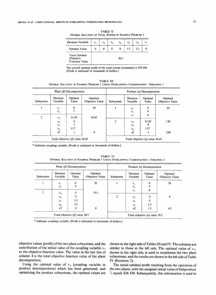
TABLE IIOPTIMAL SOLUTION OF TOTAL SYSTEM OF EXAMPLE PROBLEM 1
Decision Variable x1 X2 X3 X4 X5 x6 X7
Optimal Value 0 4 0 0 1.5 1.5 0
Total OptimalObjective 30.5Function Value
The overall optimal profit of the total system (company) is $30500.(Profit is indicated in thousands of dollars.)
TABLE IIIOPTIMAL SOLUTION OF EXAMPLE PROBLEM 1 USING OVERLAPPING COORDINATION-ITERATION 1
Decision Optimal Optimal Decision Optimal OptimalSubsystem Variable Value Objective Value Subsystem Variable Value Objective Value
I xi 0 20 1 0xi 20X24 X24
X702 0 10.5X40 2 X30 6
X5 1.5 X40X6 1.5 X61.5
X* 0 0 X* 1.5 4.5
Total objective (,B) value 30.5 Total objective (a) value 30.5
* Indicates coupling variable. (Profit is indicated in thousands of dollars.)
objective values (profit) ofthe two plant subsystems, and thecontribution of the initial value of the coupling variable X7to the objective function value. The value in the last line ofcolumn 4 is the total objective function value of the plantdecomposition.
Using the optimal value of x5 (coupling variable inproduct decomposition) which has been generated, andoptimizing the product subsystems, the optimal values are
shown in the right side ofTables III and IV. The columns aresimilar to those in the left side. The optimal value of x7,shown in the right side, is used to reoptimize the two plantsubsystems, and the results are shown in the left side ofTableIV (Iteration 2).The initial optimal profit resulting from the operation of
the two plants, with the assigned initial value ofSubproduct7, equals $26 430. Subsequently, this information is used in
73
IEEE TRANSACTIONS ON SYSTEMS, MAN, AND CYBERNETICS, VOL. SMC-10, NO. 2, FEBRUARY 1980
Prices represent dollars per thousand board feet. Sales are given as thousand board feet.
optimizing the profits from the products; the optimal profit,thus, increases to $30 430. The optimal values of the prod-ucts are then used in reoptimizing the operations of the twoplants, and the optimal profit, thus obtained, is $30 500. Thisamount is equal to the overall optimal profit ofthe company(Table II).
B. Example Problem 2
A second problem (formulation given below), similar inproblem structure to the one in Example Problem 1, is alsooptimized. Changes are made in the objective functioncoefficients, and right side; and negative coefficients are in-troduced in the constraint matrix. Complete convergence tothe overall optimal solution is obtained.The problem formulation is given by
maxf2 = 2x1 + x2 + 8x3 + 6x4 + 3x5 + 4x6 + 2x7
subject to
X- 2X2
X2
X3- 2x4 + 3x6
5x4- 4X5 - 2X6
+ 4X7 < 8
<5
<4
<6
X5 + 2X7< 3
xi>0, i=1,2,- ,7. (27)
Company management is convinced that scheduling ofpurchases and sales can be improved to increase profits.The purchase price and the selling price, as well as
maximum amounts that can be sold during each period, are
shown in Table V.The lumber and plywood are normally purchased at the
beginning of a period and sold throughout that period. Ifthelumber were stored for sale in a later period, a handling cost
of $17/1000 board ft is incurred, as well as a storage cost(including interest on invested capital) of $10/1000 board ftfor each period. The corresponding data for plywood are
$6/1000 board ft and $18/1000 board ft, respectively.A maximum of two million board ft can be stored in the
warehouse at one time (this figure includes lumber andplywood purchased for sale in the same period). Sincelumber and plywood should not age too long before sale,XYZ management wants it sold before the end of the thirdperiod.The problem can be analyzed in two ways: 1) by product
(a) decomposition, with each product presented as one
subsystem, and 2) by temporal (f,) decomposition, whereeach time period represents one subsystem.The decision variables are defined as follows.
Let x be the number of thousand board ft of lumberpurchased in period i;
y1 be the number of thousand board ft of lumbersold in period i;
zij be the number of thousand board ft of lumberstored in period i for sale in period j.
C. Example Problem 3
This example problem involves an industrial situation,analyzed by both product and temporal decomposition. Thesituation is based on a problem presented in [3].
1) Problem Statement and Formulation: The XYZ Com-pany operates a large warehouse that buys and sells lumberand plywood. Since the price of lumber and plywoodchanges during different periods of the year (three, in thiscase), the company sometimes builds up a large stock, whenprices are low, and later sells its product at higher prices.
Similar variables are defined for plywood. Let these be pi,
qi, and rij, respectively.Then the overall linear programming formulation for the
problem is
Maxf3 = -410x1 + 425y, - 430x2 + 440Y2
- 460x3 + 465Y3 - 690p + 705q1
- 715P2 + 730q2- 76Op3 + 760q3
- 17z12 -27z13 - 17Z23- 24rl 2
-42rl3- 24r23 (28)
Period
I
I i~~~~~i tf I
74
MENDU et al.: COMPUTATIONAL ASPECTS OF OVERLAPPING COORDINATION METHODOLOGY
subject toAx < c
couplingconstraints 1 1
1 1-1I -1I
1 1I I
1 -1
-1
1 -1-1I
1 11 1
1 -1
I -1
1 -
1 -1-1I
I1 -11 1
1 1
* Blanks indicate zero elements.
Equation (29) can be rearranged for product decomposition to yieldAax <Ca
coupling Iconstraints
1 1
1 1
-1 -1 1-
1 -1
1 1
1 1
1 11 1
1 -1-1I
I1 -1
-1II
-1 -1 1 -
1 -1 1 -1
1 1 1 -11 1 -1
Product 1 (lumber) Product 2 (plywood)* Indicates coupling variables in a decomposition.
This structure can be partitioned into two product subsystems (lumber and plywood). Similarly, it can also be rearrangedfor temporal decomposition to yield.
APXfi cp
1 -11 -1
L
Time period 1
* Indicates coupling variable!
-1-1
1 1 1 I1 -1 1
-1 1
1 -1-1
I1 1 1 1 1 1
1 -1 1 1
-1 1 1
1 -1 1 1
-1 1 1
_________________________________________II I
Time period 2 Time period 3
IIs.
75
Z12Z13Z23r12
r23
xIy1X2Y2X3
Y3P1q1P2q2P343
Z12Z13
Z23
3'1X2Y2
x3Y31l2r1 3r*23P1qlP2q2P3*
q3
K
K
<
K
K
<
K
K
K
200020002000
01000
00
140000
20000
80000
120000
1500
200020002000
01000
00
140000
20000
80000
120000
1500_j
(29)
(30)
x1
YlP1qlX2
Y2P2q2
12X3
Y3P3q3
7*z13z23r13r23
K<
KK
K
<K
K
K
200000
80010002000
00
140000
12002000
00
200000
15001
(31)
J L
I
I
III
I
I I
II
I-1I
I
I I
IEEE TRANSACTIONS ON SYSTEMS, MAN, AND CYBERNETICS, VOL. SMC-10, NO. 2, FEBRJUARY 1980
TABLE VIOVERALL OPTIMAL SOLUTION OF TOTAL SYSTEM OF EXAMPLE PROBLEM 3
Decision Variable z,2 Z13 z23 r2| r13 r23 xi Yi |x2 Y2 X3 Y3 PI q| P2 q2 P3 q3
Subsystem Variable Value Function Value Subsystem Variable Value Function Value
1 Z12 0 $2500 I xi 0 $-79600
:13 0 Yi 0
'23 0 PI 2000
xi 800 8000
P2 0 2 °0 $207000Y2 0 32 0
500 P2 800P3 1500 500
2 Toa0 $94400 3 (a 500 $1 157 5001
1 Al 5003r100 0
*2p 3200 1500
q, 800 *Z12 0 $-57600*p2 800 *r 2
*Z ~~023
3 *P3 0 j*rl 1200p3 1500 *r 300
Total objective for (a) value $96 900 Total objective for (13) value $96 900
*Indicates interacting variables.
This system can be partitioned into three subsystems,which relate to the three time periods.
2) Optimization: The total system (without decomposi-tion) is optimized first and yields the following optimalsolution (see Table VI).
Then, the total system using the overlapping coordinationtechnique is optimized.For the product or a decomposition, the decision vari-
ables r12, r13, r23, Pl. P2, p3 of Subsystem 2 are consideredinteracting (coupling) variables for that decomposition.This would uncouple the two product subsystems and allowindependent optimization. Note that in the present example,fixing the above decision variables has also fixed (due to theconstraint equations of Subsystem 2) the remaining decis-ion variables q1, q2, and q3 of Subsystem 2; hence, thesolution for Subsystem 2 is obtained directly. The optimal
solution (profit) for Subsystem 1 has been computed viathe simplex method.
In the temporal or ,B decomposition, the interactingvariables are Z12, Z13, Z23, r12, r13, and r23, and specifyingvalues for these variables would uncouple the three timeperiods for independent decisionmaking.The variables r12, r13, and r23 act as coupling variables in
both decompositions. Thus, selection of an initial value,different from the optimal value for these variables, wouldimply that convergence to the overall optimal solutioncannot be obtained unless there are multiple optima.To study the convergence pattern, optimization by over-
lapping coordination is performed using four different initialfeasible values for Ya y 2y 3,y3, and y4. The results aredocumented in Table VII.
Case I: y' = (0, 1200, 300, 2000, 800, O)T: Note that these
76
MENDU et al.: COMPUTATIONAL ASPECTS OF OVERLAPPING COORDINATION METHODOLOGY
TABLE VIIISUMMARY OF FINAL RESULTS-CASESES II, III, IV
Objective Function Objective FunctionValue-Iteration 1 Value-Iteration 2
Total OverallCase a-Decomposition #-Decomposition a-Decomposition Optimal Solution
II $78 002 $80 327 $80 327
III $79 659.40 $84 333.06 $84 336.06 $96 900
IV $89 966 $95 966 $95 966
values correspond to the optimal values in the total op-timized system. This case is checked to ensure that theoverlapping coordination technique does not lead to any"straying" from the optimal point.
Assigning an initial value to the coupling variables P1, P2,P3, r12, r13, r23 (i.e., amounts ofProduct 2 that can be boughtin one period, and amounts of Product 2 that are bought inone period and sold in another period) in the productdecomposition, and optimizing the two product subsystems,generate the optimal profit of $96 900. Using this informa-tion on the optimal valuesofZ12, r12, Z13, Z23, rl3, r23(whichare coupling variables in the temporal decomposition), thethree time periods are independently optimized; optimalprofit generated is $96 900 (see Table VII).The overall optimal profit and the optimal profit using
product decomposition and temporal decomposition are allequal. Thus the technique does not lead to any straying fromthe optimal point.
Note that in Case II and Case III the initial values of thecommon coupling variables in the two decompositions aredifferent from their optimal values; hence, convergence tothe overall optimal solution cannot be obtained. However,in Case IV the initial values are set at the optimal values,thereby including the possibility of convergence to theoverall optimal solution. The final results are summarized inTable VIII.The convergence levels in Case II and Case III are 84
percent and 87 percent, respectively. In Case IV, that level isabout 99 percent. Thus, with the initial values of thecommon coupling variables (r12, r13, r23) at their optimalvalue, convergence to the overall optimal solution in CaseIV is much better than in Cases II and III where an arbitraryinitial point is selected. The next section presents a morethorough discussion of such convergence.
In summary, for the example problems studied, conver-gence was either achieved by two iterations or not at all.
IV. DISCUSSION
Convergence to the overall optimum solution is obtainedin the first two example problems. In these examples the
coupling variables in the two decompositions are distinct,and they have the property that in one decomposition, oneof the coupling variables is being driven to its least possiblevalue (zero in this case), while in the other decomposition,the other coupling variable is being raised to its maximumpossible value.
In the third example problem convergence is not precisewhen the same variables (r12, r13, r2 3) are coupling variablesin both decompositions. The reason is that the variables arefixed initially and remain unchanged during the optimiza-tion process. Hence, fixing an initial value-different fromthe optimum value for these coupling variables would,unless there are multiple optima, imply that convergence tothe overall optimum cannot be obtained. In Case IV theinitial value of these coupling variables is fixed at theiroptimum value, and optimization is performed throughoverlapping coordination. Convergence is much better inthis case: the optimal objective value reaches 99 percent ofthe overall optimal objective value. Although such a levelindicates reasonably good convergence, the question re-mains: why has not complete convergence been obtained?The answer may rest with nonsatisfaction of the sufficientconditions for overall optimum convergence.The necessary condition (15), and the sufficient condition
(14) for convergence to the overall optimum may be in-terpreted in terms of a Venn diagram:
X set of all elements (matrices A, Hc,, H,) which satisfycondition (15),
Y set of all elements (matrices A, Hag PxI H,) whichsatisfy condition (14),
Z set of all problems for which convergence to theoverall optimum will be obtained.
The necessary condition (15) is checked for ExampleProblem 3 and is found to be satisfied.The sufficient condition (14) applies to a system with
equality constraints (as in Ax = c) and with variables thatare unrestricted in sign. For a system with nonnegativedecision variables, only the positive solutions of the null
77
IEEE TRANSACTIONS ON SYSTEMS, MAN, AND CYBERNETICS, VOL. SMC-10, NO. 2, FEBRUARY 1980
spaces are considered, and the condition implies that thecone formed by the total system is equal to the sum of thecones formed by the two decompositions.The next step, as mentioned above, is to check condition
(15). While not mandatory this step is advisable, as it givessome information on how strongly coupled the problem is.The sufficient condition may be checked, if the problem is aspecial type to which the condition may apply.
V. CONCLUSION
In the course of this research, the overlapping coordi-nation technique has been applied to selected exampleproblems and is shown to work well on them.
Despite some limitations imposed by the conditionswhich guarantee convergence to the overall optimum, theoverlapping coordination technique is an attractive methodfor examining a system from different viewpoints and gener-ating data for improved decisionmaking and management.
In Example Problem 1, given an initial value of thecoupling variable X7 (i.e., amount of Subproduct 7 to bemanufactured), information is generated on the profitrealized by each plant (over a changing product-mix) andeach subproduct. Such information is applicable to im-plementation of more efficient costing procedures and maylead to a more profitable mix of manufacturing facilities foreach product.Example Problem 2 slightly revises Example Problem 1.
The changes made in the coefficients of the objective func-tion, right side, and in their sign reflect the company'sdifferent operation practices over different regions. Conver-
gence is also achieved in this example problem. In ExampleProblem 3 information is generated on the profit con-tributed by each product and the profit during each timeperiod. This information may lead to better management offinances through proper budgeting.
Future research can be oriented toward the developmentof a simplified set of necessary and sufficient conditions (ifany) which would guarantee convergence to the overalloptimum.
ACKNOWLEDGMENTS
The authors thank Dr. M. R. Rao and Mr. K. Tarvainenfor their comments, Dr. M. A. H. Ruffner for her commentsand editorial assistance, and Dr. M. Buchner and Dr. KaiSung for their valuable suggestions.
REFERENCES[1] Y. Y. Haimes, Hierarchical Analyses ot Water Resources Systems:
Modeling and Optimization of Large-Scale Systems. New York:McGraw-Hill, 1977.
[2] Y. Y. Haimes and D. Macko, "Hierarchical structures in water re-sources systems management," IEEE, Trans. Syst., Man, and Cyhern.,vol. SMC-3, no. 4, pp. 396-402, 1973.
[3] F. S. Hillier and G. J. Lieberman, Introduction to Operations Research.2nd ed. San Francisco: Holden Day, 1974.
[4] D. Macko and Y. Y. Haimes, "Overlapping coordination of hierarchi-cal structures," IEEE Trans. Syst., Man, and Cvbern., vol. SMC-8, no.10, pp. 745-751, Oct. 1978.
[5] S. R. Mendu, "Applicability of overlapping coordination for linearhierarchical structures," M.S. thesis, Case Western Reserve University.Cleveland, OH, 1978.
[6] M. D. Mesarovic, D. Macko, and Y. Takahara, Theory of HierarchiculMultilevel Systems. New York: Academic, 1970.
A New Approach to Model
Structure DiscriminationMAHER S. MAKLAD AND S. T. NICHOLS, MEMBER, IEEE
Abstract In this paper a new characterization for the quality ofstochastic, linear-in-parameters, difference equations models isgiven. This requires a good model to have accurate parameterestimates and uncorrelated residues. A criterion based on thischaracterization is derived and compared with other criteria whichdepend on minimizing the mean square of model residues.
Manuscript received January 18, 1979; revised October 19, 1979. Thiswork was supported in part by Alberta Government Telephones throughan AGT Centennial Fellowship and in part by the National ResearchCouncil of Canada grant # A 7392.M. S. Maklad was with the Department of Electrical Engineering,
University of Calgary, Calgary, AB, Canada. He is now with the Depart-ment of Electrical Engineering, Queen's University, Kingston, ON, CanadaK7L 3N6.
S. T. Nichols is with the Department of Electrical Engineering, Univer-sity of Calgary, Calgary, AB, Canada T2N 1N4.
I. INTRODUCTION
M ODELING OF unknown systems and signals hasattracted a considerable deal of interest from re-
searchers with various interests. Automatic control theory,economics, biology, agriculture, and psychology aresamples of fields where models play a central role. The stateof the art has been dramatically advanced in the last decade.This is mainly due to the evolution of large digital comput-ing facilities, the advance of the state of the mathematicalsystem theory, and the appreciation of statisticalmethodology.The process of statistical model building from empirical
data consists of three stages [1]. First, select an appropriate