Computational Bodybuilding: Anatomically-based Modeling of Human Bodies Shunsuke Saito * University of Pennsylvania, Waseda University Zi-Ye Zhou † University of Pennsylvania Ladislav Kavan ‡ University of Pennsylvania Figure 1: Given an input 3D anatomy template, we propose a system to simulate the effects of muscle, fat, and bone growth. This allows us to create a wide range of human body shapes. Abstract We propose a method to create a wide range of human body shapes from a single input 3D anatomy template. Our approach is inspired by biological processes responsible for human body growth. In par- ticular, we simulate growth of skeletal muscles and subcutaneous fat using physics-based models which combine growth and elas- ticity. Together with a tool to edit proportions of the bones, our method allows us to achieve a desired shape of the human body by directly controlling hypertrophy (or atrophy) of every muscle and enlargement of fat tissues. We achieve near-interactive run times by utilizing a special quasi-statics solver (Projective Dynamics) and by crafting a volumetric discretization which results in accurate defor- mations without an excessive number of degrees of freedom. Our system is intuitive to use and the resulting human body models are ready for simulation using existing physics-based animation meth- ods, because we deform not only the surface, but also the entire volumetric model. CR Categories: I.3.7 [Computer Graphics]: Three-Dimensional Graphics—Animation Keywords: human body modeling, 3D anatomy, growth models, physics-based animation. * [email protected]† [email protected]‡ [email protected]1 Introduction Human bodies exhibit large variations in size and shape due to fac- tors such as height, muscularity, or adiposity. Although modern an- imations systems such as Weta Tissue can bring realistic digital hu- mans to life by combining physics-based simulation with detailed models of 3D anatomy, creating simulation-ready anatomical mod- els is expensive and typically involves a team of specialized digital artists experienced in 3D modeling, simulation, and anatomy. This de facto limits the applicability of realistic human body simulations to high-budget productions. In this paper, we propose a method to generate a wide range of human body shapes which are ready to be simulated using exist- ing physics-based methods. Our approach is intuitive even to inex- perienced users, because it is motivated by natural biological pro- cesses. Inspired by growth laws studied in biomechanics [Taber 1995; Taber 1998; Jones and Chapman 2012; Wisdom et al. 2015], we propose mathematical models of hypertrophy and atrophy of skeletal muscles. We devise another model for growth of fat tis- sues. Our growth models are tightly coupled with a physics-based simulation system, which accounts for elasticity of the individual organs, e.g., as the biceps muscle grows due to hypertrophy, it ex- erts forces on the adjacent tissues, pushing them out of the way. We combine our models of soft tissue growth with a geometric shape deformation technique to edit the rest pose of the body, allowing us to produce human bodies with varied anthropometry, such as heights and bone lengths. Our goal is fundamentally different from existing simulators [Lee et al. 2009] which focus on modeling the motion of the human body such as walking or lifting an object. Even though our method shares similar building blocks, e.g., volumetric elasticity and finite ele- ment methods, we simulate changes of the human body over the long term. Growth processes such as hypertrophy do not occur in- stantaneously and lead to quite different shapes than, e.g., muscle
Transcript
Computational Bodybuilding: Anatomically-based Modeling of Human Bodies
Shunsuke Saito*
University of Pennsylvania, Waseda UniversityZi-Ye Zhou†
University of PennsylvaniaLadislav Kavan‡
University of Pennsylvania
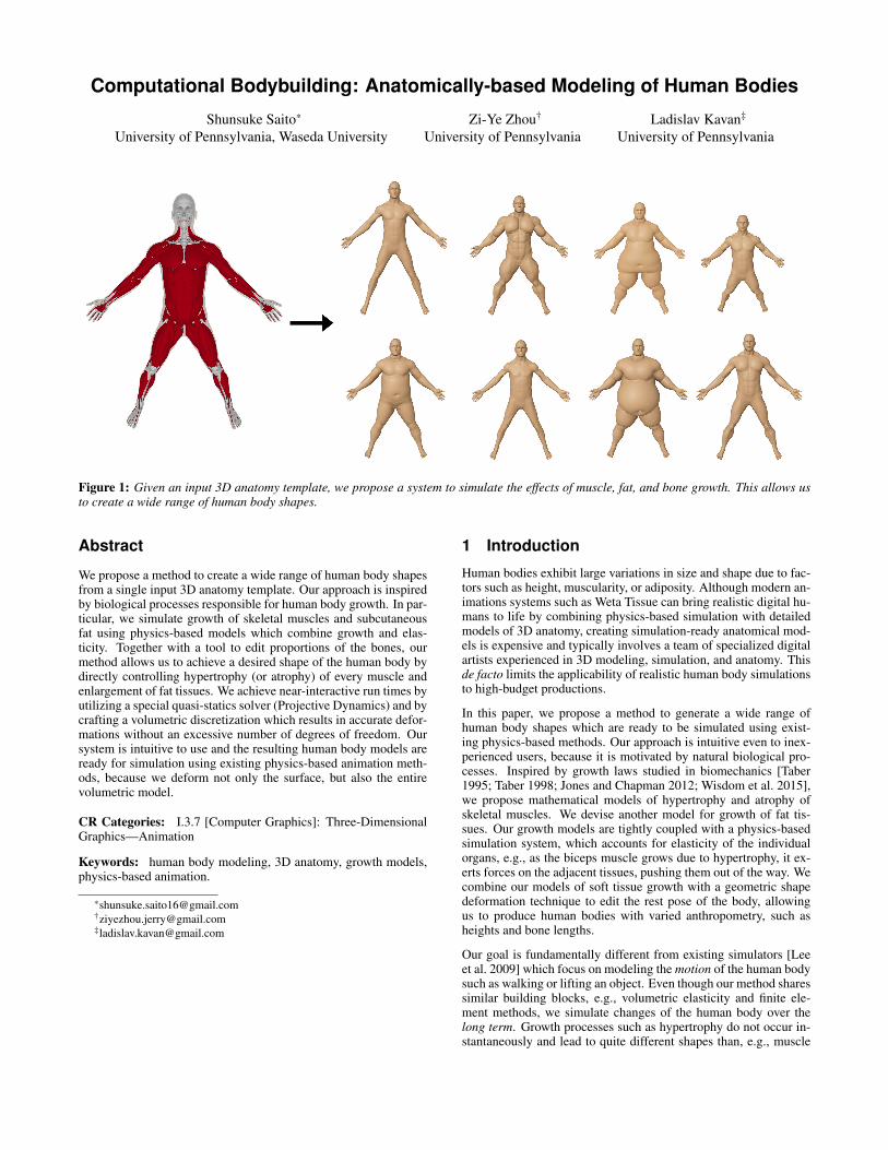
Figure 1: Given an input 3D anatomy template, we propose a system to simulate the effects of muscle, fat, and bone growth. This allows usto create a wide range of human body shapes.
Abstract
We propose a method to create a wide range of human body shapesfrom a single input 3D anatomy template. Our approach is inspiredby biological processes responsible for human body growth. In par-ticular, we simulate growth of skeletal muscles and subcutaneousfat using physics-based models which combine growth and elas-ticity. Together with a tool to edit proportions of the bones, ourmethod allows us to achieve a desired shape of the human body bydirectly controlling hypertrophy (or atrophy) of every muscle andenlargement of fat tissues. We achieve near-interactive run times byutilizing a special quasi-statics solver (Projective Dynamics) and bycrafting a volumetric discretization which results in accurate defor-mations without an excessive number of degrees of freedom. Oursystem is intuitive to use and the resulting human body models areready for simulation using existing physics-based animation meth-ods, because we deform not only the surface, but also the entirevolumetric model.
Human bodies exhibit large variations in size and shape due to fac-tors such as height, muscularity, or adiposity. Although modern an-imations systems such as Weta Tissue can bring realistic digital hu-mans to life by combining physics-based simulation with detailedmodels of 3D anatomy, creating simulation-ready anatomical mod-els is expensive and typically involves a team of specialized digitalartists experienced in 3D modeling, simulation, and anatomy. Thisde facto limits the applicability of realistic human body simulationsto high-budget productions.
In this paper, we propose a method to generate a wide range ofhuman body shapes which are ready to be simulated using exist-ing physics-based methods. Our approach is intuitive even to inex-perienced users, because it is motivated by natural biological pro-cesses. Inspired by growth laws studied in biomechanics [Taber1995; Taber 1998; Jones and Chapman 2012; Wisdom et al. 2015],we propose mathematical models of hypertrophy and atrophy ofskeletal muscles. We devise another model for growth of fat tis-sues. Our growth models are tightly coupled with a physics-basedsimulation system, which accounts for elasticity of the individualorgans, e.g., as the biceps muscle grows due to hypertrophy, it ex-erts forces on the adjacent tissues, pushing them out of the way. Wecombine our models of soft tissue growth with a geometric shapedeformation technique to edit the rest pose of the body, allowingus to produce human bodies with varied anthropometry, such asheights and bone lengths.
Our goal is fundamentally different from existing simulators [Leeet al. 2009] which focus on modeling the motion of the human bodysuch as walking or lifting an object. Even though our method sharessimilar building blocks, e.g., volumetric elasticity and finite ele-ment methods, we simulate changes of the human body over thelong term. Growth processes such as hypertrophy do not occur in-stantaneously and lead to quite different shapes than, e.g., muscle
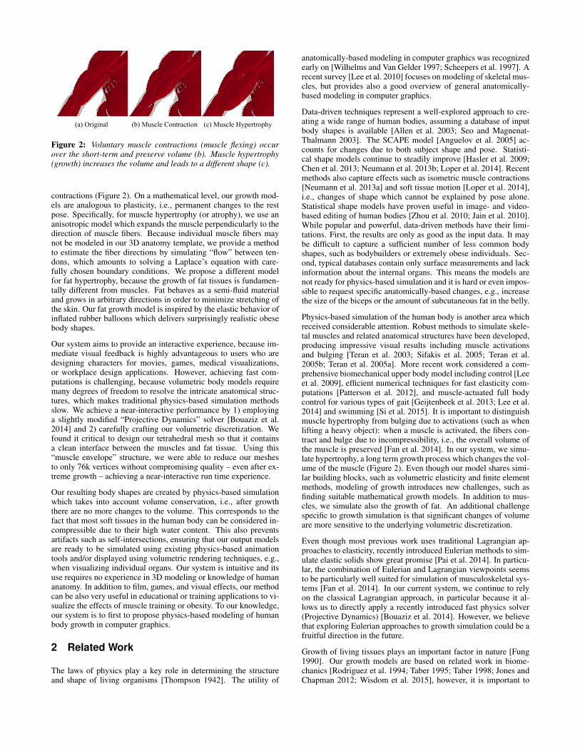
(a) Original (b) Muscle Contraction (c) Muscle Hypertrophy
Figure 2: Voluntary muscle contractions (muscle flexing) occurover the short-term and preserve volume (b). Muscle hypertrophy(growth) increases the volume and leads to a different shape (c).
contractions (Figure 2). On a mathematical level, our growth mod-els are analogous to plasticity, i.e., permanent changes to the restpose. Specifically, for muscle hypertrophy (or atrophy), we use ananisotropic model which expands the muscle perpendicularly to thedirection of muscle fibers. Because individual muscle fibers maynot be modeled in our 3D anatomy template, we provide a methodto estimate the fiber directions by simulating “flow” between ten-dons, which amounts to solving a Laplace’s equation with care-fully chosen boundary conditions. We propose a different modelfor fat hypertrophy, because the growth of fat tissues is fundamen-tally different from muscles. Fat behaves as a semi-fluid materialand grows in arbitrary directions in order to minimize stretching ofthe skin. Our fat growth model is inspired by the elastic behavior ofinflated rubber balloons which delivers surprisingly realistic obesebody shapes.
Our system aims to provide an interactive experience, because im-mediate visual feedback is highly advantageous to users who aredesigning characters for movies, games, medical visualizations,or workplace design applications. However, achieving fast com-putations is challenging, because volumetric body models requiremany degrees of freedom to resolve the intricate anatomical struc-tures, which makes traditional physics-based simulation methodsslow. We achieve a near-interactive performance by 1) employinga slightly modified “Projective Dynamics” solver [Bouaziz et al.2014] and 2) carefully crafting our volumetric discretization. Wefound it critical to design our tetrahedral mesh so that it containsa clean interface between the muscles and fat tissue. Using this“muscle envelope” structure, we were able to reduce our meshesto only 76k vertices without compromising quality – even after ex-treme growth – achieving a near-interactive run time experience.
Our resulting body shapes are created by physics-based simulationwhich takes into account volume conservation, i.e., after growththere are no more changes to the volume. This corresponds to thefact that most soft tissues in the human body can be considered in-compressible due to their high water content. This also preventsartifacts such as self-intersections, ensuring that our output modelsare ready to be simulated using existing physics-based animationtools and/or displayed using volumetric rendering techniques, e.g.,when visualizing individual organs. Our system is intuitive and itsuse requires no experience in 3D modeling or knowledge of humananatomy. In addition to film, games, and visual effects, our methodcan be also very useful in educational or training applications to vi-sualize the effects of muscle training or obesity. To our knowledge,our system is to first to propose physics-based modeling of humanbody growth in computer graphics.
2 Related Work
The laws of physics play a key role in determining the structureand shape of living organisms [Thompson 1942]. The utility of
anatomically-based modeling in computer graphics was recognizedearly on [Wilhelms and Van Gelder 1997; Scheepers et al. 1997]. Arecent survey [Lee et al. 2010] focuses on modeling of skeletal mus-cles, but provides also a good overview of general anatomically-based modeling in computer graphics.
Data-driven techniques represent a well-explored approach to cre-ating a wide range of human bodies, assuming a database of inputbody shapes is available [Allen et al. 2003; Seo and Magnenat-Thalmann 2003]. The SCAPE model [Anguelov et al. 2005] ac-counts for changes due to both subject shape and pose. Statisti-cal shape models continue to steadily improve [Hasler et al. 2009;Chen et al. 2013; Neumann et al. 2013b; Loper et al. 2014]. Recentmethods also capture effects such as isometric muscle contractions[Neumann et al. 2013a] and soft tissue motion [Loper et al. 2014],i.e., changes of shape which cannot be explained by pose alone.Statistical shape models have proven useful in image- and video-based editing of human bodies [Zhou et al. 2010; Jain et al. 2010].While popular and powerful, data-driven methods have their limi-tations. First, the results are only as good as the input data. It maybe difficult to capture a sufficient number of less common bodyshapes, such as bodybuilders or extremely obese individuals. Sec-ond, typical databases contain only surface measurements and lackinformation about the internal organs. This means the models arenot ready for physics-based simulation and it is hard or even impos-sible to request specific anatomically-based changes, e.g., increasethe size of the biceps or the amount of subcutaneous fat in the belly.
Physics-based simulation of the human body is another area whichreceived considerable attention. Robust methods to simulate skele-tal muscles and related anatomical structures have been developed,producing impressive visual results including muscle activationsand bulging [Teran et al. 2003; Sifakis et al. 2005; Teran et al.2005b; Teran et al. 2005a]. More recent work considered a com-prehensive biomechanical upper body model including control [Leeet al. 2009], efficient numerical techniques for fast elasticity com-putations [Patterson et al. 2012], and muscle-actuated full bodycontrol for various types of gait [Geijtenbeek et al. 2013; Lee et al.2014] and swimming [Si et al. 2015]. It is important to distinguishmuscle hypertrophy from bulging due to activations (such as whenlifting a heavy object): when a muscle is activated, the fibers con-tract and bulge due to incompressibility, i.e., the overall volume ofthe muscle is preserved [Fan et al. 2014]. In our system, we simu-late hypertrophy, a long term growth process which changes the vol-ume of the muscle (Figure 2). Even though our model shares simi-lar building blocks, such as volumetric elasticity and finite elementmethods, modeling of growth introduces new challenges, such asfinding suitable mathematical growth models. In addition to mus-cles, we simulate also the growth of fat. An additional challengespecific to growth simulation is that significant changes of volumeare more sensitive to the underlying volumetric discretization.
Even though most previous work uses traditional Lagrangian ap-proaches to elasticity, recently introduced Eulerian methods to sim-ulate elastic solids show great promise [Pai et al. 2014]. In particu-lar, the combination of Eulerian and Lagrangian viewpoints seemsto be particularly well suited for simulation of musculoskeletal sys-tems [Fan et al. 2014]. In our current system, we continue to relyon the classical Lagrangian approach, in particular because it al-lows us to directly apply a recently introduced fast physics solver(Projective Dynamics) [Bouaziz et al. 2014]. However, we believethat exploring Eulerian approaches to growth simulation could be afruitful direction in the future.
Growth of living tissues plays an important factor in nature [Fung1990]. Our growth models are based on related work in biome-chanics [Rodriguez et al. 1994; Taber 1995; Taber 1998; Jones andChapman 2012; Wisdom et al. 2015], however, it is important to
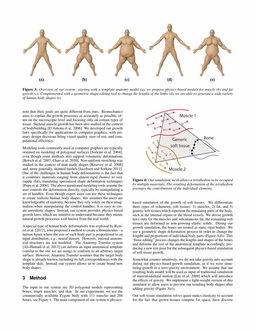
(a) (b) (c) (d) (e)
Figure 3: Overview of our system: starting with a template anatomy model (a), we propose physics-based models for muscle (b) and fatgrowth (c). Complemented with a geometric shape editing tool to change the lengths of the limbs (d), we are able to generate a wide varietyof human body shapes (e).
note that their goals are quite different from ours. Biomechanicsaims to explain the growth processes as accurately as possible, of-ten on the microscopic level and focusing only on certain types oftissue. Skeletal muscle growth has been also studied in the contextof bodybuilding [D’Antona et al. 2006]. We developed our growthlaws specifically for applications in computer graphics, with pri-mary design decisions being visual quality, ease of use, and com-putational efficiency.
Modeling tools commonly used in computer graphics are typicallyoriented on modeling of polygonal surfaces [Sorkine et al. 2004],even though some methods also support volumetric deformations[Botsch et al. 2007; Chao et al. 2010]. Non-uniform stretching wasstudied in the context of man-made shapes [Kraevoy et al. 2008]and, more generally, skinned models [Jacobson and Sorkine 2011].One of the challenges in human body deformations is the fact thatit combines materials ranging from almost rigid (bones) to verysupple (fat), mandating specialized shape deformation techniques[Popa et al. 2006]. The above mentioned modeling tools assume theuser controls the deformation directly, typically by manipulating aset of handles. Even though expert users can use these techniquesto create realistic human body shapes, this assumes the users areknowledgeable of anatomy, because they rely solely on their imag-ination when manipulating the control handles; it is easy to cre-ate unrealistic shapes. Instead, our system provides physics-basedgrowth laws, which are intuitive to understand because they mimicnatural growth processes well-known from the real world.
A special type of human body deformations was explored by Rein-ert et al. [2012], who proposed a method to create a Homunculus – ahuman figure where the size of each body part is proportional to aninput distribution, e.g., neural density. However, internal anatom-ical structures are not modeled. The Anatomy Transfer system[Ali-Hamadi et al. 2013] can deform an input anatomical template(similar to the one we are using) to conform to an arbitrary targetsurface. However, Anatomy Transfer assumes that the target bodyshape is already known, including its full correspondences with thetemplate skin. Instead, our system allows us to create brand newbody shapes.
3 Method
The input to our system are 3D polygonal models representingbones, major muscles, and skin. In our experiments we use thecommercially available Zygote body with 111 muscles and 204bones, see Figure 1. The main component of our system is physics-
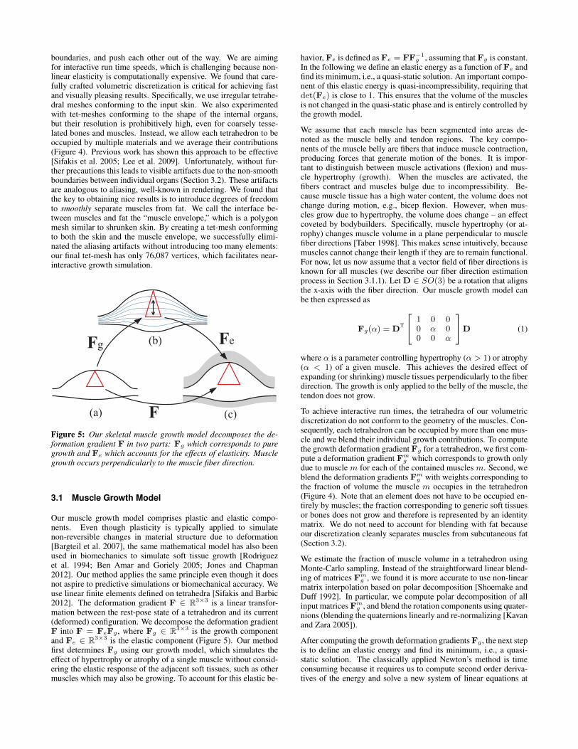
Muscle 2
Generic soft tissue
Muscle 1
Bone
Figure 4: Our simulation mesh allows a tetrahedron to be occupiedby multiple materials. The resulting deformation of the tetrahedronaverages the contributions of the individual elements.
based simulation of the growth of soft tissues. We differentiatethree types of volumetric soft tissues: 1) muscles, 2) fat, and 3)generic soft tissues which represent the remaining parts of the body,such as the internal organs or the blood vessels. We devise growthlaws only for the muscles and subcutaneous fat, the remaining softtissues are deformed as non-growing elastic solids. During ourgrowth simulation, the bones are treated as static rigid bodies. Weuse a geometric shape deformation process in order to change thelengths and proportions of individual body parts (Figure 3(d)). This“bone editing” process changes the lengths and shapes of the bonesand deforms the rest of the anatomical template accordingly, pro-ducing a new rest pose for the subsequent physics-based simulationof soft tissue growth.
Somewhat counter-intuitively, we do not take gravity into accountduring our physics-based growth simulation, as if we were simu-lating growth in a zero-gravity environment. We assume that ourresulting body model will be used as input of traditional simulationof musculoskeletal motion [Lee et al. 2009] which will introducethe effects of gravity. We implement a light-weight version of thissimulator to allow users to preview our resulting body shapes afteradding gravity (Figure 3(e)).
Our soft-tissue simulation solves quasi-statics elasticity to accountfor the fact that grown tissues compete for space, have discrete
boundaries, and push each other out of the way. We are aimingfor interactive run time speeds, which is challenging because non-linear elasticity is computationally expensive. We found that care-fully crafted volumetric discretization is critical for achieving fastand visually pleasing results. Specifically, we use irregular tetrahe-dral meshes conforming to the input skin. We also experimentedwith tet-meshes conforming to the shape of the internal organs,but their resolution is prohibitively high, even for coarsely tesse-lated bones and muscles. Instead, we allow each tetrahedron to beoccupied by multiple materials and we average their contributions(Figure 4). Previous work has shown this approach to be effective[Sifakis et al. 2005; Lee et al. 2009]. Unfortunately, without fur-ther precautions this leads to visible artifacts due to the non-smoothboundaries between individual organs (Section 3.2). These artifactsare analogous to aliasing, well-known in rendering. We found thatthe key to obtaining nice results is to introduce degrees of freedomto smoothly separate muscles from fat. We call the interface be-tween muscles and fat the “muscle envelope,” which is a polygonmesh similar to shrunken skin. By creating a tet-mesh conformingto both the skin and the muscle envelope, we successfully elimi-nated the aliasing artifacts without introducing too many elements:our final tet-mesh has only 76,087 vertices, which facilitates near-interactive growth simulation.
(b)
(a) (c)F
Fg Fe
Figure 5: Our skeletal muscle growth model decomposes the de-formation gradient F in two parts: Fg which corresponds to puregrowth and Fe which accounts for the effects of elasticity. Musclegrowth occurs perpendicularly to the muscle fiber direction.
3.1 Muscle Growth Model
Our muscle growth model comprises plastic and elastic compo-nents. Even though plasticity is typically applied to simulatenon-reversible changes in material structure due to deformation[Bargteil et al. 2007], the same mathematical model has also beenused in biomechanics to simulate soft tissue growth [Rodriguezet al. 1994; Ben Amar and Goriely 2005; Jones and Chapman2012]. Our method applies the same principle even though it doesnot aspire to predictive simulations or biomechanical accuracy. Weuse linear finite elements defined on tetrahedra [Sifakis and Barbic2012]. The deformation gradient F ∈ R3×3 is a linear transfor-mation between the rest-pose state of a tetrahedron and its current(deformed) configuration. We decompose the deformation gradientF into F = FeFg , where Fg ∈ R3×3 is the growth componentand Fe ∈ R3×3 is the elastic component (Figure 5). Our methodfirst determines Fg using our growth model, which simulates theeffect of hypertrophy or atrophy of a single muscle without consid-ering the elastic response of the adjacent soft tissues, such as othermuscles which may also be growing. To account for this elastic be-
havior, Fe is defined as Fe = FF−1g , assuming that Fg is constant.
In the following we define an elastic energy as a function of Fe andfind its minimum, i.e., a quasi-static solution. An important compo-nent of this elastic energy is quasi-incompressibility, requiring thatdet(Fe) is close to 1. This ensures that the volume of the musclesis not changed in the quasi-static phase and is entirely controlled bythe growth model.
We assume that each muscle has been segmented into areas de-noted as the muscle belly and tendon regions. The key compo-nents of the muscle belly are fibers that induce muscle contraction,producing forces that generate motion of the bones. It is impor-tant to distinguish between muscle activations (flexion) and mus-cle hypertrophy (growth). When the muscles are activated, thefibers contract and muscles bulge due to incompressibility. Be-cause muscle tissue has a high water content, the volume does notchange during motion, e.g., bicep flexion. However, when mus-cles grow due to hypertrophy, the volume does change – an effectcoveted by bodybuilders. Specifically, muscle hypertrophy (or at-rophy) changes muscle volume in a plane perpendicular to musclefiber directions [Taber 1998]. This makes sense intuitively, becausemuscles cannot change their length if they are to remain functional.For now, let us now assume that a vector field of fiber directions isknown for all muscles (we describe our fiber direction estimationprocess in Section 3.1.1). Let D ∈ SO(3) be a rotation that alignsthe x-axis with the fiber direction. Our muscle growth model canbe then expressed as
Fg(α) = DT
1 0 00 α 00 0 α
D (1)
where α is a parameter controlling hypertrophy (α > 1) or atrophy(α < 1) of a given muscle. This achieves the desired effect ofexpanding (or shrinking) muscle tissues perpendicularly to the fiberdirection. The growth is only applied to the belly of the muscle, thetendon does not grow.
To achieve interactive run times, the tetrahedra of our volumetricdiscretization do not conform to the geometry of the muscles. Con-sequently, each tetrahedron can be occupied by more than one mus-cle and we blend their individual growth contributions. To computethe growth deformation gradient Fg for a tetrahedron, we first com-pute a deformation gradient Fm
g which corresponds to growth onlydue to muscle m for each of the contained muscles m. Second, weblend the deformation gradients Fm
g with weights corresponding tothe fraction of volume the muscle m occupies in the tetrahedron(Figure 4). Note that an element does not have to be occupied en-tirely by muscles; the fraction corresponding to generic soft tissuesor bones does not grow and therefore is represented by an identitymatrix. We do not need to account for blending with fat becauseour discretization cleanly separates muscles from subcutaneous fat(Section 3.2).
We estimate the fraction of muscle volume in a tetrahedron usingMonte-Carlo sampling. Instead of the straightforward linear blend-ing of matrices Fm
g , we found it is more accurate to use non-linearmatrix interpolation based on polar decomposition [Shoemake andDuff 1992]. In particular, we compute polar decomposition of allinput matrices Fm
g , and blend the rotation components using quater-nions (blending the quaternions linearly and re-normalizing [Kavanand Zara 2005]).
After computing the growth deformation gradients Fg , the next stepis to define an elastic energy and find its minimum, i.e., a quasi-static solution. The classically applied Newton’s method is timeconsuming because it requires us to compute second order deriva-tives of the energy and solve a new system of linear equations at
(a) Without Volume Preservation (b) With Volume Preservation
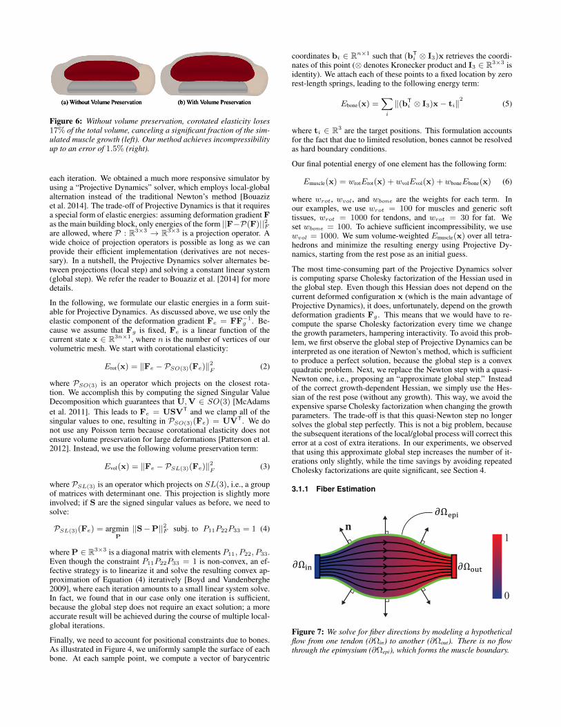
Figure 6: Without volume preservation, corotated elasticity loses17% of the total volume, canceling a significant fraction of the sim-ulated muscle growth (left). Our method achieves incompressibilityup to an error of 1.5% (right).
each iteration. We obtained a much more responsive simulator byusing a “Projective Dynamics” solver, which employs local-globalalternation instead of the traditional Newton’s method [Bouazizet al. 2014]. The trade-off of Projective Dynamics is that it requiresa special form of elastic energies: assuming deformation gradient Fas the main building block, only energies of the form ||F−P(F)||2Fare allowed, where P : R3×3 → R3×3 is a projection operator. Awide choice of projection operators is possible as long as we canprovide their efficient implementation (derivatives are not neces-sary). In a nutshell, the Projective Dynamics solver alternates be-tween projections (local step) and solving a constant linear system(global step). We refer the reader to Bouaziz et al. [2014] for moredetails.
In the following, we formulate our elastic energies in a form suit-able for Projective Dynamics. As discussed above, we use only theelastic component of the deformation gradient Fe = FF−1
g . Be-cause we assume that Fg is fixed, Fe is a linear function of thecurrent state x ∈ R3n×1, where n is the number of vertices of ourvolumetric mesh. We start with corotational elasticity:
Erot(x) = ‖Fe − PSO(3)(Fe)‖2F
(2)
where PSO(3) is an operator which projects on the closest rota-tion. We accomplish this by computing the signed Singular ValueDecomposition which guarantees that U,V ∈ SO(3) [McAdamset al. 2011]. This leads to Fe = USVT and we clamp all of thesingular values to one, resulting in PSO(3)(Fe) = UVT. We donot use any Poisson term because corotational elasticity does notensure volume preservation for large deformations [Patterson et al.2012]. Instead, we use the following volume preservation term:
Evol(x) = ‖Fe − PSL(3)(Fe)‖2F
(3)
where PSL(3) is an operator which projects on SL(3), i.e., a groupof matrices with determinant one. This projection is slightly moreinvolved; if S are the signed singular values as before, we need tosolve:
PSL(3)(Fe) = argminP
||S−P||2F subj. to P11P22P33 = 1 (4)
where P ∈ R3×3 is a diagonal matrix with elements P11, P22, P33.Even though the constraint P11P22P33 = 1 is non-convex, an ef-fective strategy is to linearize it and solve the resulting convex ap-proximation of Equation (4) iteratively [Boyd and Vandenberghe2009], where each iteration amounts to a small linear system solve.In fact, we found that in our case only one iteration is sufficient,because the global step does not require an exact solution; a moreaccurate result will be achieved during the course of multiple local-global iterations.
Finally, we need to account for positional constraints due to bones.As illustrated in Figure 4, we uniformly sample the surface of eachbone. At each sample point, we compute a vector of barycentric
coordinates bi ∈ Rn×1 such that (bTi ⊗ I3)x retrieves the coordi-
nates of this point (⊗ denotes Kronecker product and I3 ∈ R3×3 isidentity). We attach each of these points to a fixed location by zerorest-length springs, leading to the following energy term:
Ebone(x) =∑i
‖(bTi ⊗ I3)x− ti‖
2(5)
where ti ∈ R3 are the target positions. This formulation accountsfor the fact that due to limited resolution, bones cannot be resolvedas hard boundary conditions.
Our final potential energy of one element has the following form:
where wrot, wvol, and wbone are the weights for each term. Inour examples, we use wrot = 100 for muscles and generic softtissues, wrot = 1000 for tendons, and wrot = 30 for fat. Weset wbone = 100. To achieve sufficient incompressibility, we usewvol = 1000. We sum volume-weighted Emuscle(x) over all tetra-hedrons and minimize the resulting energy using Projective Dy-namics, starting from the rest pose as an initial guess.
The most time-consuming part of the Projective Dynamics solveris computing sparse Cholesky factorization of the Hessian used inthe global step. Even though this Hessian does not depend on thecurrent deformed configuration x (which is the main advantage ofProjective Dynamics), it does, unfortunately, depend on the growthdeformation gradients Fg . This means that we would have to re-compute the sparse Cholesky factorization every time we changethe growth parameters, hampering interactivity. To avoid this prob-lem, we first observe the global step of Projective Dynamics can beinterpreted as one iteration of Newton’s method, which is sufficientto produce a perfect solution, because the global step is a convexquadratic problem. Next, we replace the Newton step with a quasi-Newton one, i.e., proposing an “approximate global step.” Insteadof the correct growth-dependent Hessian, we simply use the Hes-sian of the rest pose (without any growth). This way, we avoid theexpensive sparse Cholesky factorization when changing the growthparameters. The trade-off is that this quasi-Newton step no longersolves the global step perfectly. This is not a big problem, becausethe subsequent iterations of the local/global process will correct thiserror at a cost of extra iterations. In our experiments, we observedthat using this approximate global step increases the number of it-erations only slightly, while the time savings by avoiding repeatedCholesky factorizations are quite significant, see Section 4.
3.1.1 Fiber Estimation
0
1
Ω Ω
nΩ
Figure 7: We solve for fiber directions by modeling a hypotheticalflow from one tendon (∂Ωin) to another (∂Ωout). There is no flowthrough the epimysium (∂Ωepi), which forms the muscle boundary.
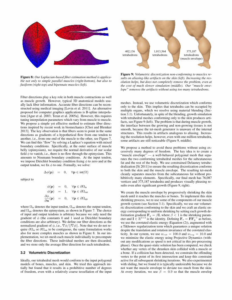
Figure 8: Our Laplacian-based fiber estimation method is applica-ble not only to simple parallel muscles (right-bottom), but also tofusiform (right-top) and bipennate muscles (left).
Fiber directions play a key role in both muscle contractions as wellas muscle growth. However, typical 3D anatomical models usu-ally lack fiber information. Accurate fiber directions can be recon-structed using medical imaging [Levin et al. 2011]. An alternativeproposed for computer graphics applications is B-spline interpola-tion [Agur et al. 2003; Teran et al. 2005a]. However, this requirestuning interpolation parameters which vary from muscle to muscle.We propose a simple yet effective method to estimate fiber direc-tions inspired by recent work in biomechanics [Choi and Blemker2013]. The key observation is that fibers seem to point in the samedirections as gradients of a hypothetical flow from one tendon toanother, i.e., from one end of the muscle to the other, see Figure 7.We can find this “flow” by solving a Laplace’s equation with mixedboundary conditions. Specifically, at the outer surface of musclebelly (epimysium), we require the normal derivative of our scalarfield φ to vanish, i.e., there is no flow through the epimysium. Thisamounts to Neumann boundary conditions. At the input tendon,we impose Dirichlet boundary condition fixing φ to zero and at theoutput tendon, we fix φ to one. Formally, we solve:
∆φ(p) = 0, ∀p ∈ int(Ω)
subject to
φ(p) = 0, ∀p ∈ ∂Ωin
φ(p) = 1, ∀p ∈ ∂Ωout
∂φ
∂n(p) = 0, ∀p ∈ ∂Ωepi
where Ωin denotes the input tendon, Ωout denotes the output tendon,and Ωepi denotes the epimysium, as shown in Figure 7. The choiceof input and output tendons is arbitrary because we only need thegradient of φ (the constants 0 and 1 used as Dirichlet boundaryconditions are also arbitrary). We define our fiber directions as thenormalized gradient of φ, i.e., ∇φ/||∇φ||. Note that we do not re-quire ∂Ωin or ∂Ωout to be contiguous, the same formulation worksalso for more complex muscles as shown in Figure 8. In our im-plementation, we tet-mesh each muscle individually to precomputethe fiber directions. These individual meshes are then discarded,and we store only the average fiber direction for each tetrahedron.
3.2 Volumetric Discretization
Ideally, our tetrahedral mesh would conform to the input polygonalmodels of bones, muscles, and skin. We tried this approach ini-tially but found that it results in a prohibitive number of degreesof freedom, even with a relatively coarse tessellation of the input
402,136tetrahedrons
1,013,564tetrahedrons
375,187tetrahedrons
(muscle envelope)
Figure 9: Volumetric discretization non-conforming to muscles re-sults on aliasing-like artifacts on the skin (left). Increasing the res-olution helps, but does not completely remove the problem, even atthe cost of much slower simulation (middle). Our “muscle enve-lope” removes the artifacts without using too many tetrahedrons.
meshes. Instead, we use volumetric discretization which conformsonly to the skin. This implies that tetrahedra can be occupied bymultiple organs, which we resolve using material blending (Sec-tion 3.1). Unfortunately, in spite of the blending, growth simulationwith tetrahedral meshes conforming only to the skin produces arti-facts, see Figure 9 (left). The problem is that during muscle growth,the interface between the growing and non-growing tissues is notsmooth, because the tet-mesh generator is unaware of the internalstructures. This results in artifacts analogous to aliasing. Increas-ing the resolution helps, however, even with one million tetrahedra,some artifacts are still noticeable (Figure 9, middle).
We propose a method to avoid these problems without using ex-cessively many degrees of freedom. The key idea is to create a“muscle envelope” — a well-behaved polygonal mesh that sepa-rates the two conforming tetrahedral meshes for the subcutaneousfat and the rest of the body. We use constrained Delauney tetrahe-dralization [Si 2011] to ensure the resulting discretization conformsto both the skin and the muscle envelope. The resulting tet-meshcleanly separates muscles from the subcutaneous fat without pro-hibitively many elements. Specifically, our final mesh has 76,087vertices and 375,187 tetrahedra and produces visually pleasing re-sults even after significant growth (Figure 9, right).
We create the muscle envelope by progressively shrinking the skinmesh until it reaches the muscles or bones. To implement this skinshrinking process, we re-use some of the components of our musclegrowth system (see Section 3.1). Specifically, we use our volumet-ric discretization conforming to the skin and we craft an elastic en-ergy corresponding to uniform shrinking by setting each growth de-formation gradient Fg = βI, where β < 1 is the shrinking param-eter and I ∈ R3×3 is the identity. Defining Fe = FF−1
g as before,we use the corotated elastic energy (Equation (2)), augmented witha Tikhonov regularization term which guarantees a unique solutiondespite the translation and rotation invariance of the corotated elas-ticity. In our system, we use wrot = 100.0 and wreg = 10.0 andwe minimize the elastic energy using Projective Dynamics (with-out any modifications as speed is not critical in this pre-processingphase). Once the quasi-static solution has been computed, we checkwhether any vertex of the shrunken skin collided with a muscle ora bone. If a collision has been detected, we constrain the offendingvertex to the point of its first intersection and keep this constraintactive for all subsequent shrinking iterations. We also experimentedwith sliding, but we found it is typically undesirable because we donot want the muscle envelope to deviate too much from the skin.At every iteration, we use β = 0.9 so that the muscle envelop
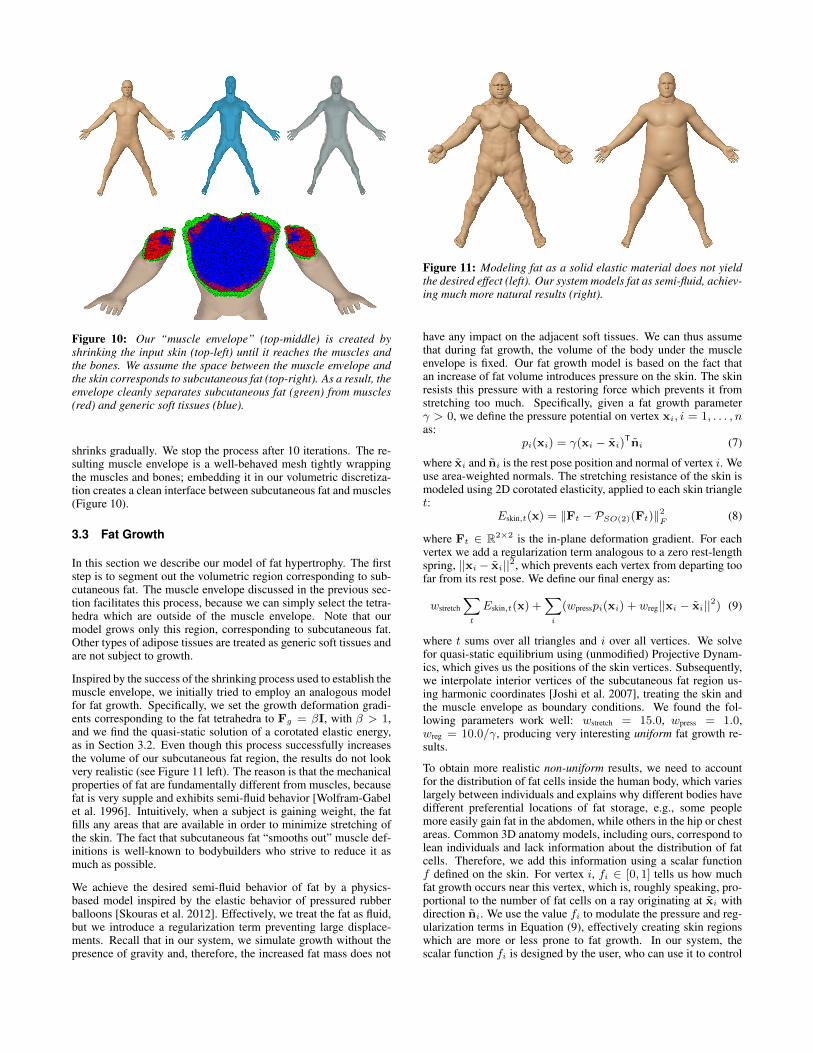
Figure 10: Our “muscle envelope” (top-middle) is created byshrinking the input skin (top-left) until it reaches the muscles andthe bones. We assume the space between the muscle envelope andthe skin corresponds to subcutaneous fat (top-right). As a result, theenvelope cleanly separates subcutaneous fat (green) from muscles(red) and generic soft tissues (blue).
shrinks gradually. We stop the process after 10 iterations. The re-sulting muscle envelope is a well-behaved mesh tightly wrappingthe muscles and bones; embedding it in our volumetric discretiza-tion creates a clean interface between subcutaneous fat and muscles(Figure 10).
3.3 Fat Growth
In this section we describe our model of fat hypertrophy. The firststep is to segment out the volumetric region corresponding to sub-cutaneous fat. The muscle envelope discussed in the previous sec-tion facilitates this process, because we can simply select the tetra-hedra which are outside of the muscle envelope. Note that ourmodel grows only this region, corresponding to subcutaneous fat.Other types of adipose tissues are treated as generic soft tissues andare not subject to growth.
Inspired by the success of the shrinking process used to establish themuscle envelope, we initially tried to employ an analogous modelfor fat growth. Specifically, we set the growth deformation gradi-ents corresponding to the fat tetrahedra to Fg = βI, with β > 1,and we find the quasi-static solution of a corotated elastic energy,as in Section 3.2. Even though this process successfully increasesthe volume of our subcutaneous fat region, the results do not lookvery realistic (see Figure 11 left). The reason is that the mechanicalproperties of fat are fundamentally different from muscles, becausefat is very supple and exhibits semi-fluid behavior [Wolfram-Gabelet al. 1996]. Intuitively, when a subject is gaining weight, the fatfills any areas that are available in order to minimize stretching ofthe skin. The fact that subcutaneous fat “smooths out” muscle def-initions is well-known to bodybuilders who strive to reduce it asmuch as possible.
We achieve the desired semi-fluid behavior of fat by a physics-based model inspired by the elastic behavior of pressured rubberballoons [Skouras et al. 2012]. Effectively, we treat the fat as fluid,but we introduce a regularization term preventing large displace-ments. Recall that in our system, we simulate growth without thepresence of gravity and, therefore, the increased fat mass does not
Figure 11: Modeling fat as a solid elastic material does not yieldthe desired effect (left). Our system models fat as semi-fluid, achiev-ing much more natural results (right).
have any impact on the adjacent soft tissues. We can thus assumethat during fat growth, the volume of the body under the muscleenvelope is fixed. Our fat growth model is based on the fact thatan increase of fat volume introduces pressure on the skin. The skinresists this pressure with a restoring force which prevents it fromstretching too much. Specifically, given a fat growth parameterγ > 0, we define the pressure potential on vertex xi, i = 1, . . . , nas:
pi(xi) = γ(xi − xi)Tni (7)
where xi and ni is the rest pose position and normal of vertex i. Weuse area-weighted normals. The stretching resistance of the skin ismodeled using 2D corotated elasticity, applied to each skin trianglet:
Eskin,t(x) = ‖Ft − PSO(2)(Ft)‖2F (8)
where Ft ∈ R2×2 is the in-plane deformation gradient. For eachvertex we add a regularization term analogous to a zero rest-lengthspring, ||xi − xi||2, which prevents each vertex from departing toofar from its rest pose. We define our final energy as:
wstretch
∑t
Eskin,t(x) +∑i
(wpresspi(xi) + wreg||xi − xi||2) (9)
where t sums over all triangles and i over all vertices. We solvefor quasi-static equilibrium using (unmodified) Projective Dynam-ics, which gives us the positions of the skin vertices. Subsequently,we interpolate interior vertices of the subcutaneous fat region us-ing harmonic coordinates [Joshi et al. 2007], treating the skin andthe muscle envelope as boundary conditions. We found the fol-lowing parameters work well: wstretch = 15.0, wpress = 1.0,wreg = 10.0/γ, producing very interesting uniform fat growth re-sults.
To obtain more realistic non-uniform results, we need to accountfor the distribution of fat cells inside the human body, which varieslargely between individuals and explains why different bodies havedifferent preferential locations of fat storage, e.g., some peoplemore easily gain fat in the abdomen, while others in the hip or chestareas. Common 3D anatomy models, including ours, correspond tolean individuals and lack information about the distribution of fatcells. Therefore, we add this information using a scalar functionf defined on the skin. For vertex i, fi ∈ [0, 1] tells us how muchfat growth occurs near this vertex, which is, roughly speaking, pro-portional to the number of fat cells on a ray originating at xi withdirection ni. We use the value fi to modulate the pressure and reg-ularization terms in Equation (9), effectively creating skin regionswhich are more or less prone to fat growth. In our system, thescalar function fi is designed by the user, who can use it to control
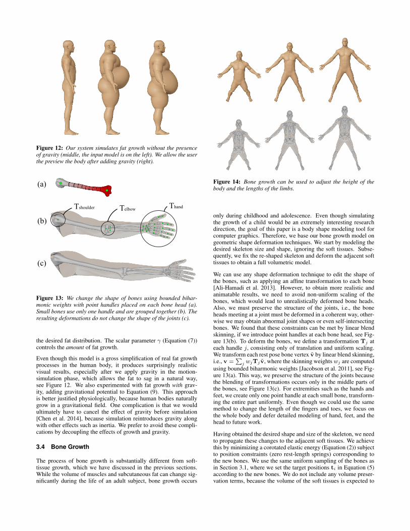
Figure 12: Our system simulates fat growth without the presenceof gravity (middle, the input model is on the left). We allow the userthe preview the body after adding gravity (right).
(a)
(b)
(c)
ThandTelbowTshoulder
Figure 13: We change the shape of bones using bounded bihar-monic weights with point handles placed on each bone head (a).Small bones use only one handle and are grouped together (b). Theresulting deformations do not change the shape of the joints (c).
the desired fat distribution. The scalar parameter γ (Equation (7))controls the amount of fat growth.
Even though this model is a gross simplification of real fat growthprocesses in the human body, it produces surprisingly realisticvisual results, especially after we apply gravity in the motion-simulation phase, which allows the fat to sag in a natural way,see Figure 12. We also experimented with fat growth with grav-ity, adding gravitational potential to Equation (9). This approachis better justified physiologically, because human bodies naturallygrow in a gravitational field. One complication is that we wouldultimately have to cancel the effect of gravity before simulation[Chen et al. 2014], because simulation reintroduces gravity alongwith other effects such as inertia. We prefer to avoid these compli-cations by decoupling the effects of growth and gravity.
3.4 Bone Growth
The process of bone growth is substantially different from soft-tissue growth, which we have discussed in the previous sections.While the volume of muscles and subcutaneous fat can change sig-nificantly during the life of an adult subject, bone growth occurs
Figure 14: Bone growth can be used to adjust the height of thebody and the lengths of the limbs.
only during childhood and adolescence. Even though simulatingthe growth of a child would be an extremely interesting researchdirection, the goal of this paper is a body shape modeling tool forcomputer graphics. Therefore, we base our bone growth model ongeometric shape deformation techniques. We start by modeling thedesired skeleton size and shape, ignoring the soft tissues. Subse-quently, we fix the re-shaped skeleton and deform the adjacent softtissues to obtain a full volumetric model.
We can use any shape deformation technique to edit the shape ofthe bones, such as applying an affine transformation to each bone[Ali-Hamadi et al. 2013]. However, to obtain more realistic andanimatable results, we need to avoid non-uniform scaling of thebones, which would lead to unrealistically deformed bone heads.Also, we must preserve the structure of the joints, i.e., the boneheads meeting at a joint must be deformed in a coherent way, other-wise we may obtain abnormal joint shapes or even self-intersectingbones. We found that these constraints can be met by linear blendskinning, if we introduce point handles at each bone head, see Fig-ure 13(b). To deform the bones, we define a transformation Tj ateach handle j, consisting only of translation and uniform scaling.We transform each rest pose bone vertex v by linear blend skinning,i.e., v =
∑j wjTj v, where the skinning weightswj are computed
using bounded biharmonic weights [Jacobson et al. 2011], see Fig-ure 13(a). This way, we preserve the structure of the joints becausethe blending of transformations occurs only in the middle parts ofthe bones, see Figure 13(c). For extremities such as the hands andfeet, we create only one point handle at each small bone, transform-ing the entire part uniformly. Even though we could use the samemethod to change the length of the fingers and toes, we focus onthe whole body and defer detailed modeling of hand, feet, and thehead to future work.
Having obtained the desired shape and size of the skeleton, we needto propagate these changes to the adjacent soft tissues. We achievethis by minimizing a corotated elastic energy (Equation (2)) subjectto position constraints (zero rest-length springs) corresponding tothe new bones. We use the same uniform sampling of the bones asin Section 3.1, where we set the target positions ti in Equation (5)according to the new bones. We do not include any volume preser-vation terms, because the volume of the soft tissues is expected to
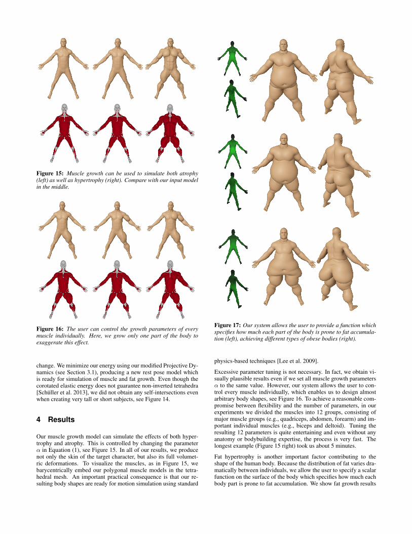
Figure 15: Muscle growth can be used to simulate both atrophy(left) as well as hypertrophy (right). Compare with our input modelin the middle.
Figure 16: The user can control the growth parameters of everymuscle individually. Here, we grow only one part of the body toexaggerate this effect.
change. We minimize our energy using our modified Projective Dy-namics (see Section 3.1), producing a new rest pose model whichis ready for simulation of muscle and fat growth. Even though thecorotated elastic energy does not guarantee non-inverted tetrahedra[Schüller et al. 2013], we did not obtain any self-intersections evenwhen creating very tall or short subjects, see Figure 14.
4 Results
Our muscle growth model can simulate the effects of both hyper-trophy and atrophy. This is controlled by changing the parameterα in Equation (1), see Figure 15. In all of our results, we producenot only the skin of the target character, but also its full volumet-ric deformations. To visualize the muscles, as in Figure 15, webarycentrically embed our polygonal muscle models in the tetra-hedral mesh. An important practical consequence is that our re-sulting body shapes are ready for motion simulation using standard
Figure 17: Our system allows the user to provide a function whichspecifies how much each part of the body is prone to fat accumula-tion (left), achieving different types of obese bodies (right).
physics-based techniques [Lee et al. 2009].
Excessive parameter tuning is not necessary. In fact, we obtain vi-sually plausible results even if we set all muscle growth parametersα to the same value. However, our system allows the user to con-trol every muscle individually, which enables us to design almostarbitrary body shapes, see Figure 16. To achieve a reasonable com-promise between flexibility and the number of parameters, in ourexperiments we divided the muscles into 12 groups, consisting ofmajor muscle groups (e.g., quadriceps, abdomen, forearm) and im-portant individual muscles (e.g., biceps and deltoid). Tuning theresulting 12 parameters is quite entertaining and even without anyanatomy or bodybuilding expertise, the process is very fast. Thelongest example (Figure 15 right) took us about 5 minutes.
Fat hypertrophy is another important factor contributing to theshape of the human body. Because the distribution of fat varies dra-matically between individuals, we allow the user to specify a scalarfunction on the surface of the body which specifies how much eachbody part is prone to fat accumulation. We show fat growth results
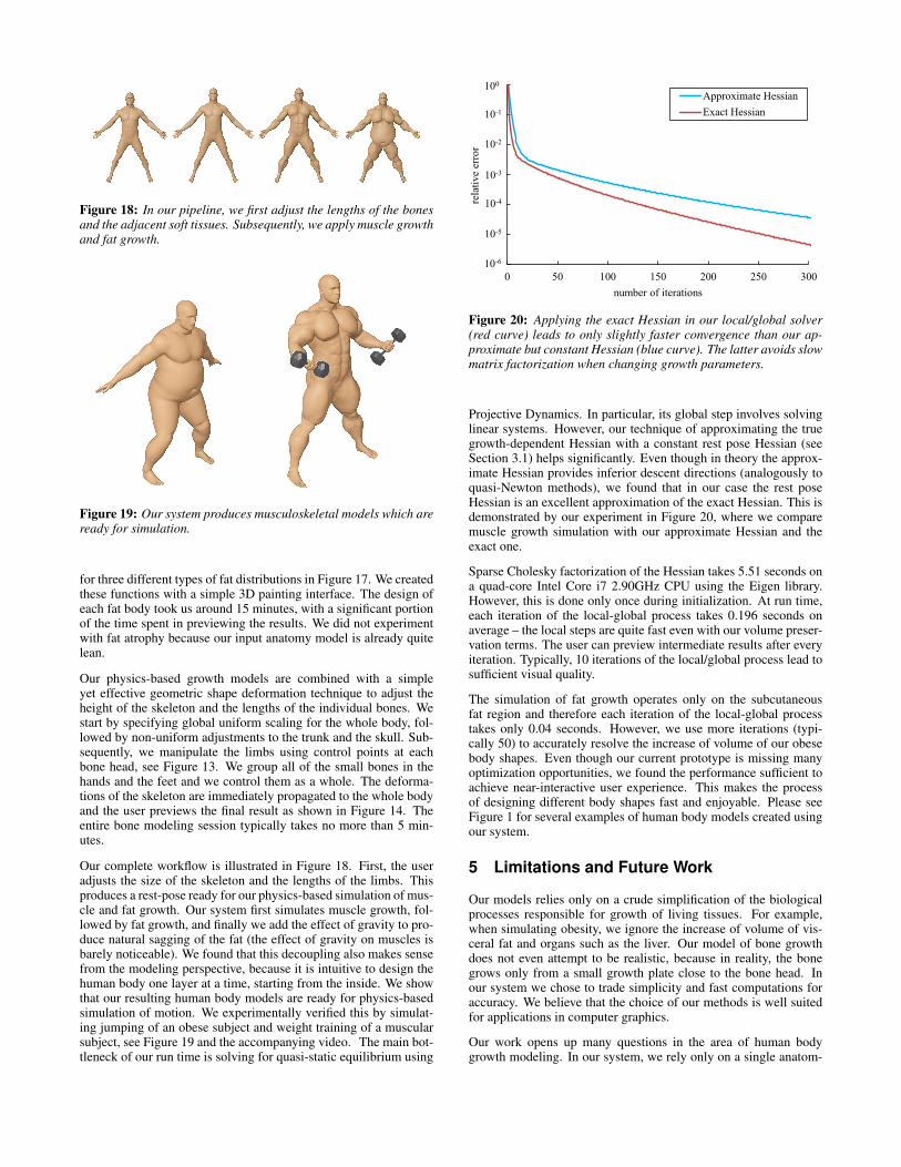
Figure 18: In our pipeline, we first adjust the lengths of the bonesand the adjacent soft tissues. Subsequently, we apply muscle growthand fat growth.
Figure 19: Our system produces musculoskeletal models which areready for simulation.
for three different types of fat distributions in Figure 17. We createdthese functions with a simple 3D painting interface. The design ofeach fat body took us around 15 minutes, with a significant portionof the time spent in previewing the results. We did not experimentwith fat atrophy because our input anatomy model is already quitelean.
Our physics-based growth models are combined with a simpleyet effective geometric shape deformation technique to adjust theheight of the skeleton and the lengths of the individual bones. Westart by specifying global uniform scaling for the whole body, fol-lowed by non-uniform adjustments to the trunk and the skull. Sub-sequently, we manipulate the limbs using control points at eachbone head, see Figure 13. We group all of the small bones in thehands and the feet and we control them as a whole. The deforma-tions of the skeleton are immediately propagated to the whole bodyand the user previews the final result as shown in Figure 14. Theentire bone modeling session typically takes no more than 5 min-utes.
Our complete workflow is illustrated in Figure 18. First, the useradjusts the size of the skeleton and the lengths of the limbs. Thisproduces a rest-pose ready for our physics-based simulation of mus-cle and fat growth. Our system first simulates muscle growth, fol-lowed by fat growth, and finally we add the effect of gravity to pro-duce natural sagging of the fat (the effect of gravity on muscles isbarely noticeable). We found that this decoupling also makes sensefrom the modeling perspective, because it is intuitive to design thehuman body one layer at a time, starting from the inside. We showthat our resulting human body models are ready for physics-basedsimulation of motion. We experimentally verified this by simulat-ing jumping of an obese subject and weight training of a muscularsubject, see Figure 19 and the accompanying video. The main bot-tleneck of our run time is solving for quasi-static equilibrium using
0 50 100 150 200 250 300
rela
tive
erro
r
number of iterations
Approximate HessianExact Hessian
100
10-1
10-2
10-3
10-4
10-5
10-6
Figure 20: Applying the exact Hessian in our local/global solver(red curve) leads to only slightly faster convergence than our ap-proximate but constant Hessian (blue curve). The latter avoids slowmatrix factorization when changing growth parameters.
Projective Dynamics. In particular, its global step involves solvinglinear systems. However, our technique of approximating the truegrowth-dependent Hessian with a constant rest pose Hessian (seeSection 3.1) helps significantly. Even though in theory the approx-imate Hessian provides inferior descent directions (analogously toquasi-Newton methods), we found that in our case the rest poseHessian is an excellent approximation of the exact Hessian. This isdemonstrated by our experiment in Figure 20, where we comparemuscle growth simulation with our approximate Hessian and theexact one.
Sparse Cholesky factorization of the Hessian takes 5.51 seconds ona quad-core Intel Core i7 2.90GHz CPU using the Eigen library.However, this is done only once during initialization. At run time,each iteration of the local-global process takes 0.196 seconds onaverage – the local steps are quite fast even with our volume preser-vation terms. The user can preview intermediate results after everyiteration. Typically, 10 iterations of the local/global process lead tosufficient visual quality.
The simulation of fat growth operates only on the subcutaneousfat region and therefore each iteration of the local-global processtakes only 0.04 seconds. However, we use more iterations (typi-cally 50) to accurately resolve the increase of volume of our obesebody shapes. Even though our current prototype is missing manyoptimization opportunities, we found the performance sufficient toachieve near-interactive user experience. This makes the processof designing different body shapes fast and enjoyable. Please seeFigure 1 for several examples of human body models created usingour system.
5 Limitations and Future Work
Our models relies only on a crude simplification of the biologicalprocesses responsible for growth of living tissues. For example,when simulating obesity, we ignore the increase of volume of vis-ceral fat and organs such as the liver. Our model of bone growthdoes not even attempt to be realistic, because in reality, the bonegrows only from a small growth plate close to the bone head. Inour system we chose to trade simplicity and fast computations foraccuracy. We believe that the choice of our methods is well suitedfor applications in computer graphics.
Our work opens up many questions in the area of human bodygrowth modeling. In our system, we rely only on a single anatom-
ical template with ad hoc material parameters. One avenue to im-prove both quality and accuracy of our models would be to use moredata acquired e.g. using MRI scanning [Fan et al. 2014]. Combin-ing our models with data-driven techniques would open a lot ofpossiblities. For example, statistical shape models of internal or-gans such as liver or kidneys could be incorporated to our modelsusing example-based materials [Martin et al. 2011]. Conversely,our model could be used to generate input for data-driven bodymodeling methods. Although we focus on growth starting from ourlean human body template, simulating weight loss of obese sub-jects would also be very interesting because skin typically does notshrink back. We did not develop detailed models for growth of theskull, hands, and feet. Growth modeling of the skull is a particu-larly important direction of future work because it could help us un-derstand and treat pathological conditions such as craniosynostosis.Even though we experimented only with a human body model, webelieve that our methods should be directly generalizable to othervertebrates and – with some modifications – to other animals. Themain hurdle in these experiments is the availability of 3D anatomi-cal models, even though recent methods such as Anatomy Transfer[Ali-Hamadi et al. 2013] aspire to alleviate this.
6 Conclusion
We presented a system to create a variety of human body shapesusing a single anatomical model as input. To our knowledge, ourwork is the first to simulate physics-based growth processes of hu-man tissues in computer graphics. We believe that our system willbe instrumental in reducing the often prohibitive costs of humanbody modeling and will find applications even beyond the tradi-tional realms of computer graphics, such as film, games, and visualeffects. For example, we envision visualization applications use-ful in bodybuilding, ergonomic analysis, or to illustrate the adverseeffects of obesity. At a higher level, we hope that our work willinspire new synergies between computer graphics and biomechan-ics.
Acknowledgements
Our special thanks belong to Sanchit Garg for designing the fatmaps and helping with rendering and video editing. We thank Mari-anne Augustine, Norm Badler, Benedict Brown, Scott Delp, JiatongHe, Xiaoyan Hu, Chuang Lan, Tiantian Liu, Shigeo Morishima,Saba Pascha, Eftychios Sifakis, Robin Tomcin, and Lifeng Zhu formany insightful discussions and the anonymous reviewers for theirvaluable comments. We also thank Harmony Li for narrating the ac-companying video. This research was supported by NSF CAREERAward IIS-1350330.
References
AGUR, A. M., NG-THOW-HING, V., BALL, K. A., FIUME,E., AND MCKEE, N. H. 2003. Documentation and three-dimensional modelling of human soleus muscle architecture.Clinical Anatomy 16, 4, 285–293.
ALLEN, B., CURLESS, B., AND POPOVIC, Z. 2003. The space ofhuman body shapes: reconstruction and parameterization fromrange scans. ACM Trans. Graph. 22, 3, 587–594.
ANGUELOV, D., SRINIVASAN, P., KOLLER, D., THRUN, S.,RODGERS, J., AND DAVIS, J. 2005. Scape: shape completionand animation of people. ACM Trans. Graph. 24, 3, 408–416.
BARGTEIL, A. W., WOJTAN, C., HODGINS, J. K., AND TURK,G. 2007. A finite element method for animating large viscoplas-tic flow. ACM Trans. Graph. 26, 3, 16.
BEN AMAR, M., AND GORIELY, A. 2005. Growth and instabilityin elastic tissues. Journal of the Mechanics and Physics of Solids53, 10, 2284–2319.
BOTSCH, M., PAULY, M., WICKE, M., AND GROSS, M. 2007.Adaptive space deformations based on rigid cells. Comput.Graph. Forum 26, 3, 339–347.
BOYD, S., AND VANDENBERGHE, L. 2009. Convex optimization.Cambridge university press.
CHAO, I., PINKALL, U., SANAN, P., AND SCHRÖDER, P. 2010.A simple geometric model for elastic deformations. ACM Trans.Graph. 29, 4, 38.
CHEN, Y., LIU, Z., AND ZHANG, Z. 2013. Tensor-based humanbody modeling. In Proc. CVPR, 105–112.
CHEN, X., ZHENG, C., XU, W., AND ZHOU, K. 2014. An asymp-totic numerical method for inverse elastic shape design. ACMTrans. Graph. 33, 4, 95.
CHOI, H. F., AND BLEMKER, S. S. 2013. Skeletal muscle fasciclearrangements can be reconstructed using a laplacian vector fieldsimulation. PloS one 8, 10, e77576.
D’ANTONA, G., LANFRANCONI, F., PELLEGRINO, M. A.,BROCCA, L., ADAMI, R., ROSSI, R., MORO, G., MIOTTI, D.,CANEPARI, M., AND BOTTINELLI, R. 2006. Skeletal musclehypertrophy and structure and function of skeletal muscle fibresin male body builders. The Journal of physiology 570, 3, 611–627.
FAN, Y., LITVEN, J., AND PAI, D. K. 2014. Active volumetricmusculoskeletal systems. ACM Trans. Graph. 33, 4, 152.
GEIJTENBEEK, T., VAN DE PANNE, M., AND VAN DER STAPPEN,A. F. 2013. Flexible muscle-based locomotion for bipedal crea-tures. ACM Trans. Graph. 32, 6, 206.
HASLER, N., STOLL, C., SUNKEL, M., ROSENHAHN, B., ANDSEIDEL, H.-P. 2009. A statistical model of human pose andbody shape. Comput. Graph. Forum 28, 2, 337–346.
JACOBSON, A., AND SORKINE, O. 2011. Stretchable andtwistable bones for skeletal shape deformation. ACM Trans.Graph. 30, 6, 165.
JACOBSON, A., BARAN, I., POPOVIC, J., AND SORKINE, O.2011. Bounded biharmonic weights for real-time deformation.ACM Trans. Graph. 30, 4, 78.
JAIN, A., THORMÄHLEN, T., SEIDEL, H.-P., AND THEOBALT,C. 2010. Moviereshape: Tracking and reshaping of humans invideos. ACM Trans. Graph. 29, 6, 148.
JONES, G. W., AND CHAPMAN, S. J. 2012. Modeling growth inbiological materials. SIAM Review 54, 1, 52–118.
JOSHI, P., MEYER, M., DEROSE, T., GREEN, B., ANDSANOCKI, T. 2007. Harmonic coordinates for character articu-lation. ACM Trans. Graph. 26, 3, 71.
KAVAN, L., AND ZARA, J. 2005. Spherical blend skinning: A real-time deformation of articulated models. In ACM SIGGRAPHSymposium on Interactive 3D Graphics and Games, 9–16.
KRAEVOY, V., SHEFFER, A., SHAMIR, A., AND COHEN-OR, D.2008. Non-homogeneous resizing of complex models. ACMTrans. Graph. 27, 5, 111.
LEE, S.-H., SIFAKIS, E., AND TERZOPOULOS, D. 2009. Com-prehensive biomechanical modeling and simulation of the upperbody. ACM Trans. Graph. 28, 4, 99.
LEE, D., GLUECK, M., KHAN, A., FIUME, E., AND JACKSON,K. 2010. A survey of modeling and simulation of skeletal mus-cle. ACM Trans. Graph. 28, 4.
LEE, Y., PARK, M. S., KWON, T., AND LEE, J. 2014. Locomotioncontrol for many-muscle humanoids. ACM Trans. Graph. 33, 6,218.
LEVIN, D. I., GILLES, B., MÄDLER, B., AND PAI, D. K. 2011.Extracting skeletal muscle fiber fields from noisy diffusion ten-sor data. Medical Image Analysis 15, 3, 340–353.
LOPER, M., MAHMOOD, N., AND BLACK, M. J. 2014. Mosh:motion and shape capture from sparse markers. ACM Trans.Graph. 33, 6, 220.
MARTIN, S., THOMASZEWSKI, B., GRINSPUN, E., AND GROSS,M. 2011. Example-based elastic materials. ACM Trans. Graph.30, 4, 72.
MCADAMS, A., ZHU, Y., SELLE, A., EMPEY, M., TAMSTORF,R., TERAN, J., AND SIFAKIS, E. 2011. Efficient elasticityfor character skinning with contact and collisions. ACM Trans.Graph. 30, 4, 37.
NEUMANN, T., VARANASI, K., HASLER, N., WACKER, M.,MAGNOR, M., AND THEOBALT, C. 2013. Capture and sta-tistical modeling of arm-muscle deformations. Comput. Graph.Forum 32, 2pt3, 285–294.
NEUMANN, T., VARANASI, K., WENGER, S., WACKER, M.,MAGNOR, M., AND THEOBALT, C. 2013. Sparse localizeddeformation components. ACM Trans. Graph. 32, 6, 179.
PAI, D. K., LEVIN, D. I. W., AND FAN, Y. 2014. Eulerian solidsfor soft tissue and more. In ACM SIGGRAPH 2014 Courses,22:1–22:151.
PATTERSON, T., MITCHELL, N., AND SIFAKIS, E. 2012. Simula-tion of complex nonlinear elastic bodies using lattice deformers.ACM Trans. Graph. 31, 6, 197.
POPA, T., JULIUS, D., AND SHEFFER, A. 2006. Material-awaremesh deformations. In Proc. of Shape Modeling International,22–22.
REINERT, B., RITSCHEL, T., AND SEIDEL, H.-P. 2012.Homunculus warping: Conveying importance using self-intersection-free non-homogeneous mesh deformation. Comput.Graph. Forum 31, 7, 2165–2171.
RODRIGUEZ, E. K., HOGER, A., AND MCCULLOCH, A. D.1994. Stress-dependent finite growth in soft elastic tissues. Jour-nal of biomechanics 27, 4, 455–467.
SCHEEPERS, F., PARENT, R. E., CARLSON, W. E., AND MAY,S. F. 1997. Anatomy-based modeling of the human musculature.In Proc. SIGGRAPH, 163–172.
SCHÜLLER, C., KAVAN, L., PANOZZO, D., AND SORKINE-HORNUNG, O. 2013. Locally injective mappings. Comput.Graph. Forum 32, 5, 125–135.
SEO, H., AND MAGNENAT-THALMANN, N. 2003. An automaticmodeling of human bodies from sizing parameters. In Proc. I3D,19–26.
SHOEMAKE, K., AND DUFF, T. 1992. Matrix animation and polardecomposition. In Proc. Graphics interface, vol. 92, 258–264.
SI, W., LEE, S.-H., SIFAKIS, E., AND TERZOPOULOS, D. 2015.Realistic biomechanical simulation and control of human swim-ming. ACM Trans. Graph. 34, 1, 10.
SI, H. 2011. A quality tetrahedral mesh generator and three-dimensional delaunay triangulator.
SIFAKIS, E., AND BARBIC, J. 2012. FEM simulation of 3D de-formable solids: a practitioner’s guide to theory, discretizationand model reduction. In ACM SIGGRAPH 2012 Courses, 20.
SIFAKIS, E., NEVEROV, I., AND FEDKIW, R. 2005. Automaticdetermination of facial muscle activations from sparse motioncapture marker data. ACM Trans. Graph. 24, 3, 417–425.
SKOURAS, M., THOMASZEWSKI, B., BICKEL, B., AND GROSS,M. 2012. Computational design of rubber balloons. Comput.Graph. Forum 31, 24.
SORKINE, O., COHEN-OR, D., LIPMAN, Y., ALEXA, M.,RÖSSL, C., AND SEIDEL, H.-P. 2004. Laplacian surface edit-ing. In Proc. SGP, 175–184.
TABER, L. A. 1995. Biomechanics of growth, remodeling, andmorphogenesis. Applied mechanics reviews 48, 8, 487–545.
TABER, L. A. 1998. Biomechanical growth laws for muscle tissue.Journal of theoretical biology 193, 2, 201–213.
TERAN, J., BLEMKER, S., HING, V., AND FEDKIW, R. 2003.Finite volume methods for the simulation of skeletal muscle. InProc. SCA, 68–74.
TERAN, J., SIFAKIS, E., BLEMKER, S. S., NG-THOW-HING, V.,LAU, C., AND FEDKIW, R. 2005. Creating and simulatingskeletal muscle from the visible human data set. IEEE Trans.Vis. Comput. Graphi. 11, 3, 317–328.
TERAN, J., SIFAKIS, E., IRVING, G., AND FEDKIW, R. 2005.Robust quasistatic finite elements and flesh simulation. In Proc.SCA, 181–190.
THOMPSON, D. W. 1942. On growth and form.
WILHELMS, J., AND VAN GELDER, A. 1997. Anatomically basedmodeling. In Proc. SIGGRAPH, 173–180.
WISDOM, K., DELP, S., AND KUHL, E. 2015. Use it or loseit: multiscale skeletal muscle adaptation to mechanical stimuli.Biomechanics and Modeling in Mechanobiology 14, 2, 195–215.
WOLFRAM-GABEL, R., BEAUJEUX, R., FABRE, M., KEHRLI,P., DIETEMANN, J., AND BOURJAT, P. 1996. Histologic char-acteristics of posterior lumbar epidural fatty tissue. Journal ofneuroradiology 23, 1, 19–25.
ZHOU, S., FU, H., LIU, L., COHEN-OR, D., AND HAN, X. 2010.Parametric reshaping of human bodies in images. ACM Trans.Graph. 29, 4, 126.


![Reconstructing Personalized Anatomical Models for Physics ...lgg.epfl.ch/publications/2016/BodyInvPhys/paper.pdf · building [Saito et al. 2015]. While Computational Bodybuilding](https://static.documents.pub/doc/80x56/5ebb6869cfbf7f23637d2d8c/reconstructing-personalized-anatomical-models-for-physics-lggepflchpublications2016bodyinvphyspaperpdf.jpg)


