COMPUTATIONAL COLOR CONSTANCY: TAKING THEORY INTO PRACTICE Kobus Barnard B.Sc. Computing Science Simon Fraser University 1990 A THESIS SUBMITTED IN PARTIAL FULFILLMENT OF THE REQUIREMENTS FOR THE DEGREE OF MASTER OF SCIENCE in the School of Computing Science @ Kobus Barnard 1995 SIMON FRASER UNIVERSITY August 1995 All rights reserved. This work may not be reproduced in whole or in part, by photocopy or other means, without the permission of the author.
Transcript
COMPUTATIONAL COLOR CONSTANCY: TAKING THEORY INTO PRACTICE
Kobus Barnard
B.Sc. Computing Science
Simon Fraser University 1990
A THESIS SUBMITTED IN PARTIAL FULFILLMENT
O F THE REQUIREMENTS FOR THE DEGREE OF
MASTER OF SCIENCE
in the School
of
Computing Science
@ Kobus Barnard 1995
SIMON FRASER UNIVERSITY
August 1995
All rights reserved. This work may not be
reproduced in whole or in part, by photocopy
or other means, without the permission of the author.
APPROVAL
Name: Kobus Barnard
Degree: Master of Science
Title of thesis: Computational Color Constancy: Taking Theory into Prac-
tice
Examining Committee: Dr. Robert F. Hadley
Chair
Dr. Stella Atkins, External Examiner
A s x i a t e Professor, Computing Science, SFU
Dr. Brian V. Funt, Senior Supervisor
Professor, cornputi&cience, SFU
bf ,G-n ian Li, Supervisor
Associate Professor, Computing Science, SFU
Date Approved:
SIMON FRASER UNIVERSITY
PARTIAL COPYRIGHT LICENSE
I hereby grant to Simon Fraser University the right to lend my thesis, project or extended essay (the title of which is shown below) to users of the Simon Fraser University Library, and to make partial or single copies only for such users or in response to a request from the library of any other university, or other educational institution, on its own behalf or for one of its users. I further agree that permission for multiple copying of this work for scholarly purposes may be granted by me or the Dean of Graduate Studies. It is understood that copying or publication of this work for financial gain shall not be allowed without my written permission.
Title of Thesis/Project/Extended Essay
Computational Color Constancy: Taking Theory into Practice
Author: (signature)
Kobus Barnard
(name)
August 16,1995
(date)
Abstract
The light recorded by a camera is a function of the scene illumination,
the reflective characteristics of the objects in the scene, and the camera
sensors. The goal of color constancy is to separate the effect of the
illumination from that of the reflectances. In this work, this takes the form of
mapping images taken under an unknown light into images which are
estimates of how the scene would appear under a fixed, known light.
The research into color constancy has yielded a number of disparate
theoretical results, but testing on image data is rare. The thrust of this work is
to move towards a comprehensive algorithm which is applicable to image
data.
Necessary preparatory steps include measuring the illumination and
reflectances expected in real scenes, and determining the camera response
function. Next, a number of color constancy algorithms are implemented,
with emphasis on the gamut mapping approach introduced by D. Forsyth and
recently extended by G. Finlayson. These algorithms all assume that the color
of the illumination does not vary across the scene. The results of these
algorithms running on a variety of images, as well as on generated data, are
presented. In addition, the possibility of using sensor sharpening to improve
algorithm performance is investigated.
The final part of this work deals with images of scenes where the
illumination is not necessarily constant. A recent promising result from
Finlayson, Funt, and Barnard demonstrates that if the illumination variation
can be identified, it can be used as a powerful constraint. However, in its
current form this algorithm requires human input and is limited to using a
single such constraint. In this thesis the algorithm is first modified so that it
provides conjunctive constraints with the other gamut mapping constraints
and utilizes all available constraints due to illumination variation. Then a
method to determine the variation in illumination from a properly
segmented image is introduced. Finally the comprehensive algorithm is
tested on simple images segmented with region growing. The results are very
encouraging.
Acknowledgments
It would have been impossible to complete this work without the help
of others. Certainly I thank my supervisor, Brian Funt, for encouraging me to
study color computer vision several years ago, and for allowing me to follow
my own interests once I started doing so. Thanks also go to all committee
members for taking the time to read yet another thesis at a busy time of year.
Most of this work follows directly from that of Graham Finlayson, and
I appreciate his patience in repeatedly explaining his contributions to me.
Mark Drew also proved to be a good resource for the mathematical parts of
computer vision. As excellent lab mates, Janet Dueck and Shubo Chatterjee
helped in many ways.
Special thanks go to Emily Butler for being supportive of my work
despite too many late night programming sessions, as well as for help with
the proof-reading.
Finally, since this work was supported by NSERC, thanks go the
Canadian tax payer.
Contents
Abstract
Acknowledgments
Contents
List of Tables
List of Figures
Introduction
Color Constancy Overview
1.1 Problem Definition
1.2 Linear Models
1.3 Chromaticity Spaces
1.4 Diagonal Transforms for Color Constancy 1.4.1 Simple Coefficient Rule Algorithms
1.4.2 The Gamut Mapping Approach
1.5 Other Algorithms
1.6 Varying Illumination Algorithms
1.6.1 The Retinex Algorithm 1.6.2 Gamut Mapping for Varying Illumination
1.7 Color Constancy on Image Data
Preliminary Measurements
2.1 Camera Calibration
2.2 Measurement of Illuminant Spectra
iii
viii
2.2 Measurement of Surface Reflectances
2.2.1 Previously Used Canonical Gamuts
Gamut Mapping Color Constancy 3.1 Overview
3.2 Implementation Details 3.2.1 Primitives
3.2.2 Gamut Mapping Implementation
3.2.3 Simple Color Constancy Algorithms
3.3 Sensor Sharpening
3.4 Results 3.4.1 Input Data
3.4.2 Format of Results
3.4.3 Sensor Sharpening Results
3.4.4 Color Constancy Simulation Results 3.4.5 Image Data Results
Color Constancy with Varying Illumination 4.1 The Varying Illumination Algorithm
4.2 Simulation Results 4.3 Finding the Illumination Map
4.4 Putting it all Together
Conclusion
Appendix A
Bibliography
vii
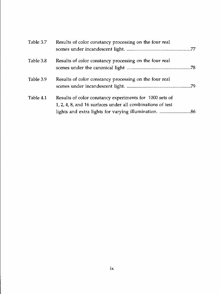
List of Tables
Table 3.1 Results of sensor sharpening tests for mapping all
responses that can be generated from the measured data
into the appropriate response for the canonical light .................... 56
Table 3.2 RGB results of sharpening experiments for 100 random
groups of 8 surfaces for each of the five test lights using
the carefully controlled image data .................................................... 58
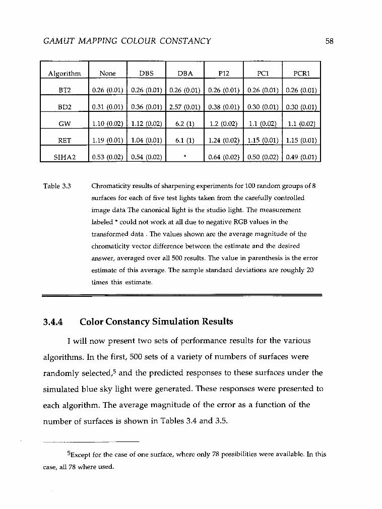
Table 3.3 Chromaticity results of sharpening experiments for 100
random groups of 8 surfaces for each of five test lights
taken from the carefully controlled image data The canonical light is the studio light ....................................................... 59
Table 3.4 Results of color constancy experiments for 500 sets of
1,2,4,6, and 8 surfaces as viewed under simulated blue
Table 3.5 Results of color constancy experiments for 500 sets of
12,16,20,24 , and 32 surfaces as viewed under simulated
blue sky light. ......................................................................................... 65
Table 3.6 Results of two-dimensional color constancy experiments
for 1000 sets of 1,2,4,8, and 16 surfaces for each of the five test lights. ........................................................................................ 66
viii
Table 3.7 Results of color constancy processing on the four real
scenes under incandescent light ........................................................ 77
Table 3.8 Results of color constancy processing on the four real
scenes under the canonical light ....................................................... 78
Table 3.9 Results of color constancy processing on the four real
scenes under incandescent light ........................................................ 79
Table 4.1 Results of color constancy experiments for 1000 sets of
1.2.4.8. and 16 surfaces under all combinations of test
lights and extra lights for varying illumination ............................ 86
List of Figures
Figure 1.1 Visualization of the first part of the gamut mapping
Figure 2.1 Camera response functions as determined by the methods
described in this section. ...................................................................... 31
Figure 2.2 Chromaticity gamut of all measured illumination. ...................... 33
Figure 2.3 Chromaticity gamuts of sets of measured surfaces under a
Philips CW fluorescent light as viewed by the Sony CCD ................................................................................................... camera. ..35
Figure 2.4 Chromaticity gamuts of the measured data together with
the gamuts for the published Krinov and Munsell data ............................................................................................................ sets. 36
Figure 2.5 Chromaticity gamut of the Munsell data set showing the
distribution of chromaticities .............................................................. 37
Figure 3.1 Illustration of multiple constraints on the mapping from
the unknown illuminant to the canonical. ..................................... 41
Figure 3.2 The illumination chromaticity gamut showing the data
points used to estimate the inverse hull .......................................... 43
Figure 3.3
Figure 3.4
Figure 3.5
Figure 3.6
Figure 3.7
Figure 3.8
Figure 4.1
Figure 4.2
Figure 4.3
Figure 4.4
Results of color constancy processing on the Macbeth color
checker viewed under the vision lab overhead light .................... 68
Illumination gamut mapping constraints for Macbeth color checker under the vision lab overhead light
algorithm [For90], and Finlayson's recent simplification and extension
[Fin95]. All these algorithms assume that the illumination does not vary
across the scene, except for Finlayson's which assumes that the chromaticity
of the illumination does not vary. Since coefficient rules are restricted cases
of linear transformations such that the corresponding post multiplication
matrix is diagonal, coefficient rules are equally referred to as diagonal
transforms.
It has been observed that the suitability of diagonal transforms is
partly a function of the sensors. Overlap, linear independence, and most
importantly, sharpness are considerations (see, for example, [BWSl, WB82,
For901). Intuitively, if the sensors are delta functions, then the diagonal
transform model follows directly from equation (1.1). Going further,
Finlayson et. al. [FDF94a, FDF94bl have shown that by applying the
appropriate linear transforms to the data, the coefficient rule can be made to
work better; in essence, the sensors are "sharpened". This original work was
based on published sensor functions which purport to model human cone
responses.
To explain further the nature of the computation, let T be a matrix (to
be determined) of the same dimension as the number of sensors. Let U be a
matrix whose rows are the pixel RGB values of the image under the
unknown illuminant. Then the transformed data is UT. (Using post
6 [ ~ ~ ~ 7 5 ] has an adjustment to the basic computation which makes Retinex a non-
coefficient rule. This adjustment was added in response to measurements of the human visual
system. It is not a reasonable way to implement Retinex in the case of linear camera.
COLOUR CONSTANCY OVERVIEW
multiplication for the mappings proves to be more natural). On the
assumption that a diagonal model is now more applicable, we apply a
coefficient rule algorithm with UT as input. The result of a coefficient rule
algorithm is a diagonal matrix D (with the coefficients along the diagonal).
Once we are done, our estimate C, for the pixel RGB values under the
canonical illuminant is given by:
c = UTDT-I (1.6)
It should be noted that applying sharpening leads to an non-coefficient
rule algorithm, since TDT-' is not normally diagonal. Thus one way to look
at sharpening is that it allows one to use a more powerful mapping function,
but apply well motivated coefficient rule based algorithms. We must be able
to do better using this approach, simply because the identity matrix is a
possible candidate for T. Some of the available methods for calculating T are
discussed in 53.3.
The majority of the algorithms explored in this thesis are coefficient
rules. As part of this research I verified that the camera sensors are already
quite sharp in the sense that the best possible diagonal result is within 1O0/0 of
that which can be obtained with sharpening. Thus good results should be
obtainable without sharpening. Nonetheless, sharpening the camera sensors
was explored as part of this research. The initial goal was simply to maximize
the performance of the algorithms, and the assumption was that sharpening
sensors that were already quite sharp would either have negligible effect, or a
small beneficial effect. Instead it was found that applying sharpening to this
domain was complicated, with the effect being a function of the algorithms,
the sharpening method, and the particular data used to derive the transform
COLOUR CONSTANCY OVERVIEW 11
(see s3.4.3). Hence the unambiguous success with the human cones did not
immediately carry over to the camera sensors, and more work is required to
reap any benefits that may be possible.
1.4.1 Simple Coefficient Rule Algorithms
Several coefficient rule algorithms can be classified as simply
normalizing the three channels by some method. The algorithm of Brill and
West [BW81] normalizes by a patch determined to be white. The grey world
algorithm assumes that the average reflectivity of the scene is that of middle
grey. This is the hypothesis used by Buchsbaum [Buc80] in the context of
linear models.7 Assuming that diagonal models are adequate, the coefficients
of each channel are normalized by twice the average of all the pixel values of
that channel. Finally, if the Retinex algorithm is applied to a scene with no
illumination variation, then each channel is normalized by the maximum
in each channel. All these algorithms can easily be shown to be inadequate.
They all fail, for example, if the scene is completely red. It could be argued
that this is a bleak situation for any color constancy algorithm to face, but
these algorithms simply do not recognize when it is better to do nothing, and
thus can give anomalous results.
1.4.2 The Gamut Mapping Approach
The gamut mapping approach was introduced by Forsyth [For90], and
has recently being modified and extended by Finlayson [Fin95]. The gamuts
7~uchsbaum was restricted to the same number of dimensions as sensors. The
inaccuracies incurred doing this are larger than assuming a diagonal model, in the case of our
camera sensors. In addition, the small dimensional model is assumed to hold for two consecutive
calculations, increasing the error even more.
COLOUR CONSTANCY OVERVIEW 12
that are mapped are the set of all sensor responses that are physically possible
under a given light. The gamut mapping approach views coefficient color
constancy as saying that changes in illumination correspond to diagonal
mappings between the gamuts. In other words, the sensor responses possible
under an unknown light are transformed to the sensor responses possible
under the canonical light by an independent scaling of each component. The
sensor responses observed under the unknown light restrict the mappings
which are possible. Since the sensor response for a light can be defined as the
sensor response of a perfect white surface as seen under that light, the
diagonal mappings between gamuts will equally be mappings between lights.
Thus a compact statement of the idea is to constrain the possible mappings
taking the unknown illuminant to the canonical illuminant. Once this
mapping is determined, we simply apply it to the unknown image to
produce the sensor response for the scene under the canonical light. A few
more details are given below.
First, it is important that the gamuts are convex. A single pixel sensor
may sample light from more than one surface. If we assume that the
response is the sum of the responses of the two contributing pieces, and that
the response due to each of these is proportional to their area, then it is
possible to have any convex combination of the responses. Thus the gamut
of all possible sensor responses to a given light must be convex.
Since the gamuts are convex, they will be represented by their convex
hulls. Now consider the RGBfs in the image taken under an unknown light.
These must be in the entire gamut for the unknown illuminant. Since we
are modeling illumination changes by diagonal transforms, each of these
measured RGBfs must be mapped into the canonical gamut by the
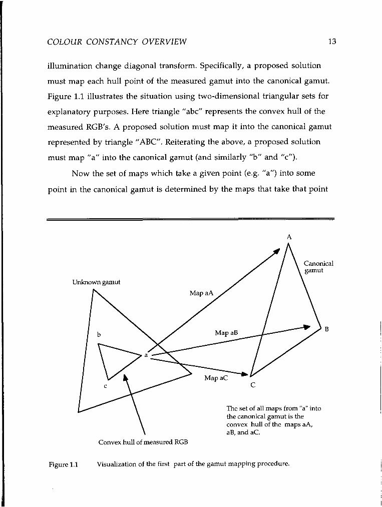
COLOUR CONSTANCY OVERVIEW 13
illumination change diagonal transform. Specifically, a proposed solution
must map each hull point of the measured gamut into the canonical gamut.
Figure 1.1 illustrates the situation using two-dimensional triangular sets for
explanatory purposes. Here triangle "abc" represents the convex hull of the
measured RGBfs. A proposed solution must map it into the canonical gamut
represented by triangle "ABC". Reiterating the above, a proposed solution
must map "a" into the canonical gamut (and similarly "b" and "c").
Now the set of maps which take a given point (e.g. "a") into some
point in the canonical gamut is determined by the maps that take that point
Unknown gamut
The set of all maps from "a" into the canonical gamut is the convex hull of the maps aA, aB, and aC.
Convex hull of measured RGB
Figure 1.1 Visualization of the first part of the gamut mapping procedure.
COLOUR CONSTANCY OVERVIEW
All maps taking "b" into the / canonical gamut.
All maps taking "c" into the
All maps taking "a" into the canonical gamut.
The intersection of the three sets of mappings is the set of mappings taking the entire unknown into the canonical gamut.
Figure 1.2 Visualization of the second part of the gamut mapping procedure.
into the hull points of the canonical gamut. If we use vectors to represent the
mappings from the given point to the various canonical hull points, then
we seek the convex hull of these vectors. It is critical to realize that we have
introduced a level of abstraction here. We are now dealing with geometric
properties of the mappings, not the gamuts. It is easy to verify that it is
sufficient to consider the mappings to the hull points (as opposed to the
entire set), by showing that any convex combination of the maps takes a
given point into a similar convex combination of the canonical hull points.
COLOUR CONSTANCY OVERVIEW 15
The final piece of the logical structure is straightforward. Based on a
given point ("a" in our example), we know that the mapping we seek is in a
specific convex set. The other points lead to similar constraints. Thus we
intersect the sets to obtain a final constraint set for the mappings. Figure 1.2
illustrates the process.
Recently Finlayson proposed using the gamut mapping approach in
chromaticity space, reducing the dimensional complexity of the problem
from three to two in the case of trichromats [Fin95]. Not all chromaticity
spaces will work. However, Finlayson showed that if the chromaticity space
was obtained by dividing each of two sensor responses by a third, as in the
case of (red/blue, greedblue), then convexity is maintained where required.
One advantage to working in a chromaticity space is that the algorithm is
immediately robust with respect to illumination intensity variation. Such
variation is present in almost every image, as it originates from the
ubiquitous effects of shading and nearby, extended light sources.
Furthermore, highlights due to specular reflection do not present trouble in
chromaticity space, because here they behave as very white surfaces (this
assumes that they do not saturate the camera sensors).
In addition to using chromaticity space, Finlayson added an important
new constraint. Not all theoretically possible lights are commonly
encountered. From this observation, Finlayson introduced a constraint on
the illumination. The convex hull of the chromaticities of the expected
lights makes up an illumination gamut. Unfortunately, the corresponding
set of allowable mappings from the unknown gamut to the canonical gamut
is not convex (it is obtained from taking the component-wise reciprocals of
COLOUR CONSTANCY OVERVIEW 16
the points in the above convex set). Nonetheless, Finlayson was able to apply
the constraints in the two dimensional case. In the work that follows the
convex hull of the non-convex set was simply taken, as it was found to be a
satisfactory approximation both for the two-dimensional and three-
dimensional case.
Other Algorithms
A few approaches to color constancy only peripherally related to this
work should be at least mentioned to provide some balance. Foremost, at
least historically, is the Maloney-Wandell algorithm [MW86, Wan871. This
approach is based on the small dimensional linear models defined in s1.2.
They found that one could solve for the components of the light vector
provided that the surface dimensionality is less than the number of the
sensors. In the case of three sensors, this forces us to assume that the
reflectances are two dimensional. Assuming two dimensional reflectances,
the sensor responses under a fixed, unknown light will fall in a plane. The
orientation of this plane indicates the illumination. Despite its significance,
the Maloney-Wandell algorithm does not work very well [FF94, FFB951. The
first reason is simple: the dimensionality of surfaces is greater than two. The
algorithm is also not very robust with insufficient data. For example, if there
is essentially one color in the scene, then the sought after plane is entirely
free in one of its two degrees of freedom (the plane is anchored at the origin).
Gershon et. al. [GJT86] were able to use an additional dimension for
surfaces by incorporating an average scene reflectance assumption similar to
the grey world assumption. Here the average reflectance of the scene is
COLOUR CONSTANCY OVERVIEW 17
determined by averaging the RGB's of distinct regions. This overcomes the
weakness of the grey world assumption when applied to a scene
predominantly one (non-grey) color, provided that other colors are available
in smaller proportions. The expected scene reflectivity is determined by
averaging published reflectance data. This algorithm relies on several
optimistic assumptions. First, in the usual trichromatic case, it is assumed
that surfaces can be described by three basis functions. Second, the average
reflectance of the scene is that given by averaging the published data set.
Although this is a step beyond the simple grey world hypothesis, no
mention is made of any attempts to verify this assumption.
Another interesting approach involves modeling the specular and
diffuse parts of scene reflectance [Sha85]. For most practical situations, this
cannot be used as one's sole method of color constancy processing. However,
this idea will likely be very useful for a complete color constancy system. For
now it has to be left as a tantalizing possibility for future work.
Finally, in the course of this research, I studied the probabilistic
approaches initiated by Vhrel and Trussel [VT91], and researched extensively
by Brainard and Freeman [BF94, FB951. The thrust of the work is estimating
the reflectance and illumination factors from their observed product, in the
face of measurement error, with access to a priori estimates of reflectance and
illumination likelihoods. The problem of obtaining these likelihoods is not
addressed, and therefore a large part of the color constancy problem is
ignored. They provide the results of simulations where they compare their
algorithm to others, but the data is generated with a method favorable to
their algorithm. Their model assumes that the components of a small
COLOUR CONSTANCY OVERVIEW
dimensional model for surfaces and illumination will follow a Gaussian
distribution, and they test the algorithm against such input. Although it is
common to generate data for simulations, it is a problem here because there
is no additional justification for the key assumption. Nonetheless, it would
be interesting to see this algorithm tested against real data.
Varying Illumination Algorithms
The preceding algorithms assume that the illumination, or at least its
chromaticity, is constant over the scene. Only a few algorithms try to deal
with the reality that this is often not the case. An important part of this thesis
deals with the varying illumination problem, and the relevant algorithms
are introduced here to provide some context.
1.6.1 The Retinex Algorithm
In theory, Land's Retinex algorithm [LM71, MMT75, Lan77, Lan861 can
deal with varying illumination. The Retinex algorithm emerged from work
on the human visual system, and treating it as a computational color
constancy algorithm takes some care. On the basis of psychophysical
experiments showing that perceived lightness is influenced by edges, Land
and his colleagues proposed a simple scheme in which illumination
variation is removed from lightness computation. Thus the motivation was
not to extend an algorithm to deal with an additional challenge, but to
model human vision. This may explain the anomaly that despite the
implicit promise of dealing with varying illumination, the test of Retinex
which is most comparable to tests of computational color constancy
COLOUR CONSTANCY OVERVIEW
algorithms was done on scenes where the illumination variation was
carefully minimized.8
In the Retinex algorithm, the basic idea is that changes in
illumination can be distinguished from changes in surface reflectance by the
assumption that reflectance changes are spatially abrupt, whereas
illumination changes will occur gradually. Thus reflectance changes can be
determined simply by identifying jumps larger than some threshold value.
In Retinex the reflectivity of a given location is determined relative to a
bright spot by taking a random path from the location in question. This path
must not intersect itself. With luck (or with a complex enough path), a patch
for each channel which is close to the maximum, brightness possible for that
channel will be crossed. The results for a number of these paths are averaged
to reduce the error.
An algorithm based on these random walks is arguably inelegant. For
one, the results are irreproducible. Horn [Hor74] realized that the essence of
the matter was differentiation (to identify the jumps), followed by
thresholding (to separate reflectance from illumination), followed by
integration (to recover lightness). It should be noted that this method uses
the logarithm of the pixel values. This can also be implemented by using . The difficulty with this method is that the two-dimensional integral does
not necessarily exist. Funt et. al. [FDB92] developed a method to insure the
8This is best explained in [MMT75]. The same experiment is also referred to in [Lan77],
but some details relevant to this work are omitted. The scenes were illuminated indirectly
through the walls of an integrating cube. Using this method, the illumination variation would
be far less than that in the real scenes used in this thesis.
COLOUR CONSTANCY OVERVIEW
existence of the integral in a slightly different context. The problem can also
be approach using homomorphic filtering. [GW87] Another approach to the
problem will be introduced as part of this work.
1.6.2 Gamut Mapping for Varying Illumination
Recently Finlayson et. al. [FFB95] introduced a new approach to the
problem of varying illumination. Rather than accepting illumination
variation as a hindrance to be removed, it was found that it could provide a
powerful constraint. Certainly the information provided by seeing the same
surface under different illumination has been studied, but primarily only in
the context of seeing the entire scene under two different illuminants at
different times; the illumination for each such view is assumed uniform
(see [T090, ZI93, Fin941). One method available for using varying
illumination without multiple views is in the case of chromaticity shifts at a
shadow boundary [FF94]. This method requires shadows in the scene, and
more critically, some external method to identify them.
In [FFB95] it is observed that in chromaticity space the mappings from
unknown illumination to a canonical illuminant fall nearly on a straight
line. This corresponds to the illuminant chromaticities lying on a curve,
since they are inverted to produce the mappings. This is congruent with the
observation the chromaticities of the 10 illuminants used lie approximately
on the Planckian locus. This set of mappings produces a set of chromaticities
defining possibilities for the sensor responses of the surface under the
canonical illuminant. Since the computation is simply a scaling, the mapped
set is also a line. A second view produces a second line. Provided the
illuminations are indeed different in chromaticity, and the system's sensors
COLOUR CONSTANCY OVERVIEW
are adequate, these lines will intersect, providing a single estimate of the
surface chromaticity under the canonical light.
As promising as this method is, there is still much to be done. First,
the problem of identifying the appropriate surface is not dealt with. Second,
since we are concerned with scenes where the illumination varies
substantially, it is not safe to assume that the solution for one appropriate
surface (a wall, for example), propagates without modification to other parts
of the scene (a bookshelf, for example). Also it is quite optimistic to assume
that every part of a scene will be close enough to an appropriate surface. On a
similar track, if there is little variation in the illumination chromaticity,
then the algorithm will fail. Third, the lines obtained are justified on the
assumption that the chromaticities of the lights lie roughly on a particular
curve. This leaves open the question of how to handle a wider illumination
set. In short, we have a kernel of a solution that must be integrated into a
more comprehensive system.
Chapter four of this thesis deals with this integration. The algorithm
is modified to work together with the gamut mapping algorithms based on
surface and illumination constraints described in 51.4.2. In this extension,
the entire illumination gamut is used, overcoming the commitment to one
approximation for the expected illumination. Then the problem of
identifying the illumination variation is solved in the case of easy to
segment images. The results obtained are very encouraging.
COLOUR CONSTANCY OVERVIEW
Color Constancy on Image Data
The eventual goal of computational color constancy is effective and
robust color constancy processing on image data. Experiments on generated
data are necessary to evaluate ideas, but the eventual goal implies that
testing should be done on real data as soon as possible. If this is not done,
algorithms suitable only for generated data may be favored. Furthermore, it
seems natural to point the camera at some part of the world and test one's
algorithms on that input, and it is a little surprising how few results of this
sort are available. This may be due, in part, to the brittleness of computer
vision algorithms when run on arbitrary data.
Although they do not use a camera, some of the work of Land and his
associates qualifies as being tested on "real" datag. There is human
interaction, but all the steps that are not automated could easily be
automated. The system must deal with noise and other varieties of bad data,
as well as non-conformance to theoretical models. It should be noted,
however, that all the work is with well behaved images with lots of color
(very carefully illuminated patchworks of rectangular pieces of matte paper
dubbed "Mondrians").
David Forsyth tested his algorithm on a number of color Mondrians
[For90]. He also writes about the absence of tests on real data, coming up with
a few instances of single tests (page 16). Since the algorithms he
9~ince their research focus is on human vision, they estimate cone responses for the
image locations and use this for input to a computer program [MMT75].
COLOUR CONSTANCY OVERVIEW 23
implemented will work using each pixel as a surface patch, I assume this was
done. He does not, however, provide this information.
Finally, Tominaga reports results from image data from a camera with
six sensors implemented by using a monochrome CCD in conjunction with
six narrow band filters [Tom94]. In addition, the dynamic range was extended
by taking pictures at various shutter speeds. A combination of the Maloney-
Wandell approach with the dichromatic modeling of Shafer was
implemented. The results reported were for cylinders covered with colored
paper as well as plastic ones.
If we accept the philosophy put forth at the beginning of this section,
then the current lack of carefully controlled results on image data suggests
that such results should be desirable. In this thesis, results on image data are
provided for four scenes (included one which can be described as arbitrary)
viewed under three different illuminants. The algorithms tested under the
same conditions include two simple coefficient rules and eight variations of
gamut mapping algorithms. Results are also provided for image data under
varying illumination, but here the results are presented graphically and
visually, since algorithms that could compete under the same conditions
have not been implemented.10 In conclusion, the results presented in this
thesis are a healthy contribution to the embarrassingly small set of careful
tests on image data.
1 • ‹~he only candidate would be the Retinex algorithm.
Chapter Two
Preliminary Measurements
In order to address the issues of color constancy on real images, the
nature of the input to the RGB values as defined by (1.1) must be investigated.
To this end, real world lighting and surface reflectances, as well as the camera
sensor functions, were measured.
2.1 Camera Calibration
In theory it is possible to implement all the algorithms tested as part of
this work without knowing the camera response functions (assuming that
they are modeled by (1.1)), but in practice it is exceedingly convenient if they
are known. Once the model has been verified, and the sensor functions
determined, it is possible to generate the canonical gamuts and test data with
far less effort than doing so directly. This is due in part to the fact that it is
easier to obtain high quality measurements with a modern spectraradiometer
than with the camera. In a sense, camera calibration is a process where the
PRELIMINARY MEASUREMENTS 25
camera is used very carefully once, and then the results are used to predict the
responses.
If we let C(A) = S(A)E(A), and restrict our consideration to only one
channel, then (1 .l) becomes:
The goal is to determine R(A) from a number of p and C(A) pairs. If we could
produce nicely spaced color signals which were very sharp, then the response
function would be sampled exactly at the peak locations, and a smooth curve
could be fit through the result. This approach is not used because it is difficult
to produce such color signals with enough energy, and such that the signal is
uniform over a sufficient number of pixels.1 Instead a method inspired by
Sharma and Trussel's approach [ST941 is used.
To begin, we represent the continuous functions by vectors whose
components are the sampling of the functions at equally spaced intervals.
Since the spectraradiometer measures from 380nm to 780nm in steps of 4nm,
these vectors will have 101 components, with the first component being the
value at 380nm, the second component being the value at 384nm, and so on.
Using R for the reflectance vector, and C for the color signal vector, equation
(2.1) becomes:
p = R O C
l1f this method is to be used, then the best approach is to use a set of interference
filters. This was used by Tominaga [Tom941 with reasonable success. Nonetheless, a better use of
such filters would be to use them in conjunction with the method explained shortly.
PRELIMINARY MEASUREMENTS 26
The strategy in camera calibration is to probe the camera with a
number of different C , to get a number of different responses, and to use this
to estimate R. Thus we have a number of equations:
p ( k ) = R. ~ ( k ) (2.3)
Due to the large dimensionality of the vectors (101), and the small
dimensionality of the signals, the system of equations in (2.3) is severely
under-constrained. It is part of the challenge of calibrating the camera to
produce unnatural illuminants to increase the dimensionality of the space of
the c ' ~ ) . Even so, the set of equations is expected to be under-constrained.
Sharma and Trussel introduce additional constraints. First they insist that the
response functions are non-negative. Second, they introduce smoothness
constraints. These take the form of bounds on a discrete estimation of the
second derivative:
* - - R 5 6 (Except for first and last Ri) (2.4)
Next they constrain the maximum error:
Ip(*) - R ~ " ' 1 5
Finally, they constrain the sum of squares error:
Sharma and Trussel then observe that the constraint sets are all convex, and
propose that the method of projection onto convex sets (POCS) be used to
characterize the result. They use their method to obtain a good estimate for
the sensitivity of a color scanner.
PRELIMINARY MEASUREMENTS
However, we can do a little better with less effort, given that
implementing POCS would be an involved process, as an external program
for this method could not be found. First, it is convenient to rewrite (2.5) as:
2*Ri - Ri-, - Ri+, I 6, (Except for first and last Ri)
Ri-I - Ri+, - 2*Ri I 6, (Except for first and last Ri) (2.8)
Here I have introduced separate constraints on the lower and upper limits on
the second derivative. Since we expect the sensors to be positive, uni-peaked
functions, the absolute value of an acceptable upper limit is more than that
for the lower limit. Next it would seem preferable to minimize the left hand
side of (2.5), rather than constrain the error interval. In fact, for our purposes,
it is better to minimize the sum of squares relative error:
This amounts to finding the best least squares solution to MR=l, where
the rows of M are the vectors c'~' scaled by P'~', subject to the above
constraints. At this stage, we have a least squares fit problem with linear
constraints. For this problem, implementations of standard numerical
solution methods are readily available.2 If it is preferred, implementing the
minimization of absolute error is even easier, and minimizing a weighted
sum of both is also simple.
21 used the DBOCLS routine in the SLATEC math library available by anonymous FTP
from netlib2.cs.utk.edu.
PRELIMINARY MEASUREMENTS 28
The experimental set up consisted of a Sony DXC-930 CCD camera with
a Canon zoom lens, a Photoresearch 650 spectraradiometer, and a number of
lights, surfaces, and filters used to craft a set of C with as high a dimension as
possible. The camera settings were chosen to be as neutral as possible. Most
importantly, the gamma adjustment was turned off. It is necessary to have
the camera sensor gains set either for daylight (color balanced to 5400K) or
indoor light (color balanced to 3200K), and the choice was made to use the
latter (3200K). It was discovered that the camera-digitizer system has an offset
of roughly 13 RGB units. In other words, if there is absolutely no light
reaching the camera, it records RGB vectors with mean (11.1, 13.2, 12.9) and
standard deviations of the order of 2.5. Values well outside the standard error
do occur, but it was found that the mean and standard errors are consistent
over a period of months. It is critical to subtract such an offset from camera
RGBfs for practically all color constancy processing (whenever equation (1.1) is
assumed to hold). The standard deviation of the offset is taken to be
indicative of the sensor error due to noise.
Preliminary measurements verified that the camera is linear within
5%. These were done by increasing the intensity of light reaching the camera
by moving a bright light closer to a standard white reflectance seen both by the
camera and the spectraradiometer (at essentially the same angle). The camera
response was found to increase linearly with the incident light energy, as
measured by the spectraradiometer. Preliminary measurements also verified
that there are small, but not entirely negligible effects on the chromaticity
recorded by the camera under extreme changes in the optics. The magnitude
of the camera sensor functions will, of course, change with the aperture, but
PRELIMINARY MEASUREMENTS 29
there are also slight changes in the chromaticity with both aperture changes
and focal length changes. These effects differ across the viewing field, and are
mostly confined to the outer half of the field of view. The results provided
are for an aperture setting of 2.8, a focal length of 25, and the central 10% of
the field of view. The aperture control is too coarse for good reproducibility.
Thus the camera sensor curves will predict camera responses for an aperture
that is only estimated by 2.8. For our research, this slight uncertainty is not a
problem. It would be a problem if the aperture changed during the calibration.
For this reason, the aperture ring was taped firmly in place during the
measurements.
The procedure was to measure alternately the light coming from some
combination of lights, surfaces, and filters, with both the camera and the
spectraradiometer. In order that the geometry was kept constant, the
spectraradiometer was mounted on top of the camera, which itself was on a
tripod. Switching between the two sampling devices was achieved by raising
and lowering the tripod head. Based on several dry runs, and the
examination of many spectra, a collection of light-surface-filter combinations
was chosen which provided close to the most variation possible with the
equipment at hand. The lights include an incandescent light, a Philips CW
fluorescent light, a slide projector, and a black light (a strong source of
ultraviolet light close to the visible spectrum). The surfaces consisted of the
Macbeth color checker patches and 19 paint chips. The filters were Kodak
gelatin filters 29 (red), 58 (green), 47A (light-blue), and 47B (blue). Again due
to previous experience, not all possible light-surface-filter combinations were
PRELIMINARY MEASUREMENTS
used, as there is much redundancy in them. In the final run 58 combinations
were used.
In order to determine the final camera response, a number of pixels in
the area of interest were averaged. The size of the area used is a compromise.
The larger the area, the more illumination variation and optical problems
there will be. In addition, the pixels will correspond, on average, to points
further from the small sampling region of the spectraradiometer. On the
other hand, as the area is decreased, more noise and other error is introduced,
and it is possible that the sampling region of the spectraradiometer could be
missed entirely. For this work, a region which was roughly five times the size
of the sampling area of the spectraradiometer was used. This produced image
sections of a few hundred pixels.
Computing the sensor functions by the method above is somewhat of
an art. We do not know what the functions are, but on the other hand, we
assume that we know roughly what they look like. Basically we assume that
they start at zero, rise smoothly to a peak, fall smdothly back to zero, and stay
there. By imposing these constraints, we hope to better model the actual
sensors, and thus gain power in predicting the response to spectra quite
different from the test set. If we were only interested in spectra close to the test
set, a straight minimization of the error would suffice (the curves produced
doing this are very jagged). By adjusting the balance between smoothness and
minimum error, a set of smooth curves which predict the camera response
over the test set to within 3% RMS relative error were found. The RMS
absolute error is 3.5 pixel values. Since the minimum error possible with the
non-negativity constraints is about 2%, this is a good fit. The sensor curves
are shown in Figure 2.1.
PRELIMINARY MEASUREMENTS
Sonv CCD Camera Sensors Estimate
Red sensor - Green sensor
Blue sensor - - - - -
fit: minimum rms relative error second derivative min: -15.0 -16.0 -20.0 second derivative max: 150.0 200.0 150.0 max value outside range: 0.10 0.10 0.10 allowed red range: 500-700 allowed green range: 456-620 allowed blue range: 380-780 camera offset: 11 . I 13.2 12.9
400 500 600 700 800 Wavelength (nanometers)
Figure 2.1 Camera response functions as determined by the methods described in this
section. The functions are only valid for an aperture setting of 2.8 and camera
settings of 3200K, no gain adjustment, and no gamma correction.
Measurement of Illurninant Spectra
As described in g1.5.2, restricting the set of expected illuminations is a
powerful constraint. This leads to the problem of what constitutes an
appropriate restriction on the illumination. Finlayson [Fin951 used the
published data for the 6 phases of daylight UMG641 (D48, D55, D65, D75, D100,
and D220), the standard CIE illuminants A, B, and C, a 2000K Planckian black
body radiator, and uniform white. Thus it was established that a reasonably
large set of illuminants is still small enough to be a good constraint.
PRELIMINARY MEASUREMENTS
However, to have confidence that the algorithm will work on real images,
one needs to know if the illumination set includes all lights deemed
''typical". In addition, it may be possible to make the constraint set smaller. If
this was the case, knowing real world lighting would improve the
performance of some of the algorithms.3
It is possible through the use of filters, or by bouncing light off deeply
colored objects, to construct a set of "lights" which is so large as to be useless
as a constraint. But the set of lights must include all lights expected in the
application domain; otherwise, the constraint will work artificially well when
tested on included lights, and may fail when tested on the excluded ones.
Despite the lack of a good definition of "typical" illumination, I set out
to measure it. The lighting was measured at various places in and around the
SFU campus, at various times of the day, and in a variety of weather
conditions. Unusual lighting, such as that beside neon advertising lights, was
excluded. However, care was taken to include some reflected light. It seems
fair to include lighting which has some component reflected from a concrete
building, but not if the building was painted pink. Similarly, the light
underneath trees was included. Altogether, roughly 100 different spectra were
measured. The chromaticities of the measured spectra are shown in
Figure 2.2.
31n some sense this turned out to be the case. Although including a wide range of
illuminants expanded Finlayson's gamut in some directions, no light as red as 2000K was
encountered, and hence the measured gamut was more restrictive in the red.
PRELIMINARY MEASUREMENTS
Chromaticity Gamuts 1.2 , , I I I 1 I I I I I
,*? Chromaticities 0 I I ,' I
Convex Hull , . 1
Figure 2.2 Chromaticity gamut of all measured illumination.
Measurement Surface Reflectances
In spite of a wealth of published surface reflectance data, surface
reflectances were also measured for several reasons. First, one important set
of data, the Krinov data set [Kri47], only includes reflectances for wavelengths
from 400nm to 650nm. The other data sets are restricted to the range of 400nm
to 700nm. Figure 2.1 shows that the camera sensors respond to wavelengths
outside these ranges. Second, in the case of the Macbeth color checker which
was used for many experiments, it makes sense to use the reflectances of our
copy, rather than assume that they are as published. By far the most
important impetus for measuring reflectances was that the color of some
PRELIMINARY MEASUREMENTS 34
objects in our lab did not fall inside the gamut of the published data. An
underlying assumption of the gamut mapping algorithms is that the
canonical gamuts include responses for all surfaces. If this assumption does
not hold, then the algorithms can perform poorly (as was the case). In
summary, spectra were measured for essentially the same reason that
illumination was measured-to ensure that the properties of the real world
were accounted for.
To measure reflectances, the spectra of light reflected from a surface
was divided by the spectra of light reflected from a barium oxide standard
white surface purchased from Photoresearch. The incident light angle was
45", and measurements were taken at an angle of 90". Since it was found that
it was virtually impossible to illuminate even a relatively small area evenly,
it was critical to make sure that the standard reflectance and the test
reflectance were in the same place.
The goal was not to produce a complete set of measurements, but
simply to validate the use of the published data, and to extend it where
necessary. Thus most surfaces were chosen based on how different they were
from ones already measured. In addition, a few surfaces that were suspected
of causing problems for our color constancy algorithms were measured. The
surfaces measured included the Macbeth color checker patches, some paint
chips, the covers of some books used in our test scenes, some brightly colored
shirts, and a number of pieces of construction paper. In total, 78 surfaces were
measured. The chromaticity gamuts of these sets of surfaces as viewed under
a Philips CW fluorescent bulb are shown in Figure 2.3.
PRELIMINARY MEASUREMENTS
Figure 2.3 Chromaticity gamuts of sets of measured surfaces under a Philips CW
fluorescent light as viewed by the Sony CCD camera.
Chromaticity Gamuts
In Figure 2.4 the measured gamuts are combined into one gamut, which is
4.5
4
3.5
compared to the published data sets. The interesting point is that the
I I I I I I 4
Gamut due to 7 books - /I. Gamut due to 22 colored pa ers - - .,' t, Gamut due to 7 samples of cToth -I:' -
, ' .... :: Gamut due to Macbeth Colour Checker ------.--. i ,.....,"
,.:T ; Gamut due to 19 paint chips ... . . - ,...- , i
/ I ' .... ...' , )
,' ..'. ! i
measured gamut does extend outside what is available in the published data
I' ....
3 -
e M
(in the lower right). Furthermore, extension of the gamut in this direction
cannot be explained by the lack of data for wavelengths less than 400nm. A
second point of interest is the great extent to which the Munsell chip gamut
exceeds the measured gamut in the blue direction. This anomaly is primarily
due to a small number of points. In other words, the great majority of the 462
PRELIMINARY MEASUREMENTS
Chrornatiaty Gamuts I I I 1 I I
Gamut due to measured reflectances - Gamut due to published Krinov data
Gamu! due to published Munsell data - - - - - , .
Figure 2.4 Chromaticity gamuts of the measured data together with the gamuts for the
published Krinov and Munsell data sets.
surfaces are inside the measured gamut, and a few are far outside it.4 This can
be seen in Figure 2.5 which shows the distribution of the chromaticities in the
Munsell chip gamut. Since these surfaces have a very small amount of blue,
this could be explained by the cutoff in the measurement range, but the
spectral characteristics of the surface would be odd. Other explanations that
should be ruled out include a problem with the Munsell measurements, or
other standard sources of error. Still, the likeliest explanation is that these
4 ~ h e Munsell chip data used is the set of 462 spectra measured by Nickerson [Nic57].
Spectra 131 and 428 were far outside the measured gamut. Spectra 91, 129, 130,458 were a little
outside, and 6 other spectra were slightly outside.
PRELIMINARY MEASUREMENTS
Chromaticity Gamuts 8 t I I I I I 1
Chromaticities o Convex Hull I
Figure 2.5 Chromaticity gamut of the Munsell data set showing the distribution of
chromaticities.
colors do exist in paint chips. Although it technically goes against the
philosophy of my approach, the rarity of the offending colors both in the data
set, and in the lab, justifies using the measured gamut for convenience. On
the other hand, the large extra piece of the gamut due to the Munsell chips
does indicate that additional effort spent building (and checking) the
reflectance databases is warranted.
2.2.1 Previously Used Canonical Gamuts
Having established the source of the gamuts used in this research, the
gamuts used in previous work should be mentioned. In contrast to our
approach of generating the gamuts from measured spectra and calibrated
PRELIMINARY MEASUREMENTS 38
camera sensors, Forsyth determined his gamut by taking pictures under a real,
physical, canonical light [For90]. For surfaces he used a collection of 180
colored pieces of paper. Finlayson, on the other hand, generated his gamut
from the reflectances of the Macbeth color checker, and then expanded the
gamut by 5% to account for the possibility out of gamut chromaticities [Fin95].
Chapter Three
Gamut Mapping Color Constancy
The focus of this part of the research is the implementation of a
number of color constancy algorithms in the same framework, in order that
meaningful comparisons and observations can be made. Essentially all
published algorithms are correct in the sense that if the author's model holds,
the expected results will be forthcoming. The problem in going from
theoretical to practical situations is that the assumptions, many of which are
implicit, often do not hold. But if we compare algorithms (or dare to rank
them), then we are saying that we can define a fair input set. Nonetheless, an
important first step is to test the algorithms in the same context, and attempt
to evaluate the relevant features of the results as they pertain to our
necessarily biased input.
Of specific interest in this chapter is the relationship between the three-
dimensional approach and the two-dimensional approach, the methods for
GAMUT MAPPING COLOUR CONSTANCY 40
choosing a solution from the constraint set, and the usefulness of sensor
sharpening.
Overview
The general idea of the gamut mapping approach is to constrain the set
of solutions. We can apply constraints determined from the sensor responses,
henceforth referred to as surface or S constraints, and intersect them for a
solution set. In three dimensions this is Forsyth's method [For90]. We can
additionally intersect this solution set with the illumination constraint, as
done by Finlayson in two dimensions. Figure 3.1 illustrates the utilization of
multiple constraints in the two-dimensional case. Some specific solutions are
also plotted.
Implementation Details
3.2.1 Primitives
In order to discuss the details of the algorithms, it is helpful to be able
to refer to a few primitive operations. The foremost of these is finding the
convex hull of a set of points. This was achieved by using the program qhull
modified so that the hull computation was callable from C pr0grams.l
Fortuitously, qhull provides the facet normals as well as the hull points.
Second, it was necessary to compute hull intersections in 2 and 3 dimensions,
and for this, a simple approximation was used. First the bounds in all
l ~ h u l l is available by anonymous FTP from geom.umn.edu
GAMUT MAPPING COLOUR CONSTANCY
Two Dimensional Dtagonal Gamut Mappings I 1 1 - - 1 I 1 --7
S constraint b..- S Cppstfiint 7
.S.Constraint 8 ---.- .... I Constraint ..........
lntersdiibn of S Conswaint(s) - Inrerbction I and S Constraint(s) -
This final equation is at the heart of the method. Here we have conditions on
the map component for two of the regions. Other boundary points produce
additional equations. In order to have a robust method, one would like long
boundaries to have more weight in the process than short ones, since the
latter may due to a small region consisting entirely of noise. But this is exactly
what we will get if we enter one equation for each boundary pair, and solve
the resulting system of equations in the least squares sense. Furthermore,
some boundary pairs can be identified as being of high quality, and these are
weighted even more by scaling the equation by a number greater than one
(typically five). In addition, some boundary pairs should contribute less, and
COLOR CONSTANCY WITH VARYING ILLUMINATION 89
their equations are scaled by a number less than unity. These lesser quality
pairs arise dealing with the pitfall described next.
In order to have a solution to the set of equations, it must be ensured
that all segments connect to each other through the boundary pairs. This can
be accomplished by simply assigning a region to every point, and using each
break in both the horizontal and vertical directions to produce a boundary
pair. This is usually not an option because normally some parts of the image
should not be used. For example, the area may be too dark. Therefore
connectedness was enforced in the following manner. Boundary pairs were
assigned at each horizontal and vertical change of region. If one of the regions
was to be ignored, a good region was sought in the same direction, taking as
many pixels as required. The resulting equation was weighted inversely to the
distance taken to find a good region. Thus such a boundary would contribute
little to the solution, but connectivity was not a problem.2
As mentioned above, there is some variation in boundary pair quality.
It was found to be better to use pixels one unit towards the insides of the
respective regions, if these were available. This way the pixels would tend to
have contributions that were solely due to a single surface, as opposed to the
possibility that they sampled over more than one surface. These boundary
pairs were weighted by a factor of five compared to ones where it was
necessary to use pixels exactly on the boundary.
2 ~ s i n g this method, it is still possible to have an unconnected image. However, these
are well defined and are not likely to occur in practice. Thus this possibility was ignored. For
the image to still be unconnected, it would need a cross of unassigned pixels extending from side
to side, and top to bottom, dividing it into four sections.
COLOR CONSTANCY WITH VARYING ILLUMINATION
Putting it all Together
The methods of the preceding sections were tested on three real
images. In all cases the scenes were illuminated by an incandescent desk light
on the left, and simulated blue sky on the right. Thus the test covered a
common real world situation-an office with a window. All scenes were
chosen to produce images which were easy to segment, as the segmentation
method used cannot handle complex images. Figure 4.1 shows the first scene
illuminated as described above. Figure 4.2 shows the segmentation and all
points that contribute to the boundary pairs (in red). The boundary areas are
quite wide for two reasons. First 20% resolution was used for computation.
Second, as described in s4.3, whenever possible boundary pairs were taken
one unit inside the regions. Figure 4.3 shows the image with the illumination
chromaticity variation removed, and Figure 4.4 shows the illumination map
deduced. The input for color constancy processing is this image (for the
surface constraints), and the illumination map (for the varying illumination
constraints). Figure 4.5 shows the result of color constancy processing. The
input is reproduced in the upper left corner. Unlike the images in s3.4, the
upper right corner is the result of applying surface and illumination
constraints. The lower left corner is the result of applying these constraints
and the varying illumination constraints, and the lower right is the same
scene under the canonical illuminant (Phillips CW fluorescent). Due to a
fortuitous selection of colors, the varying illumination constraints are almost
superfluous in this case, as both algorithms do well. It is important to note
that even if the varying illumination constraints are not needed, the
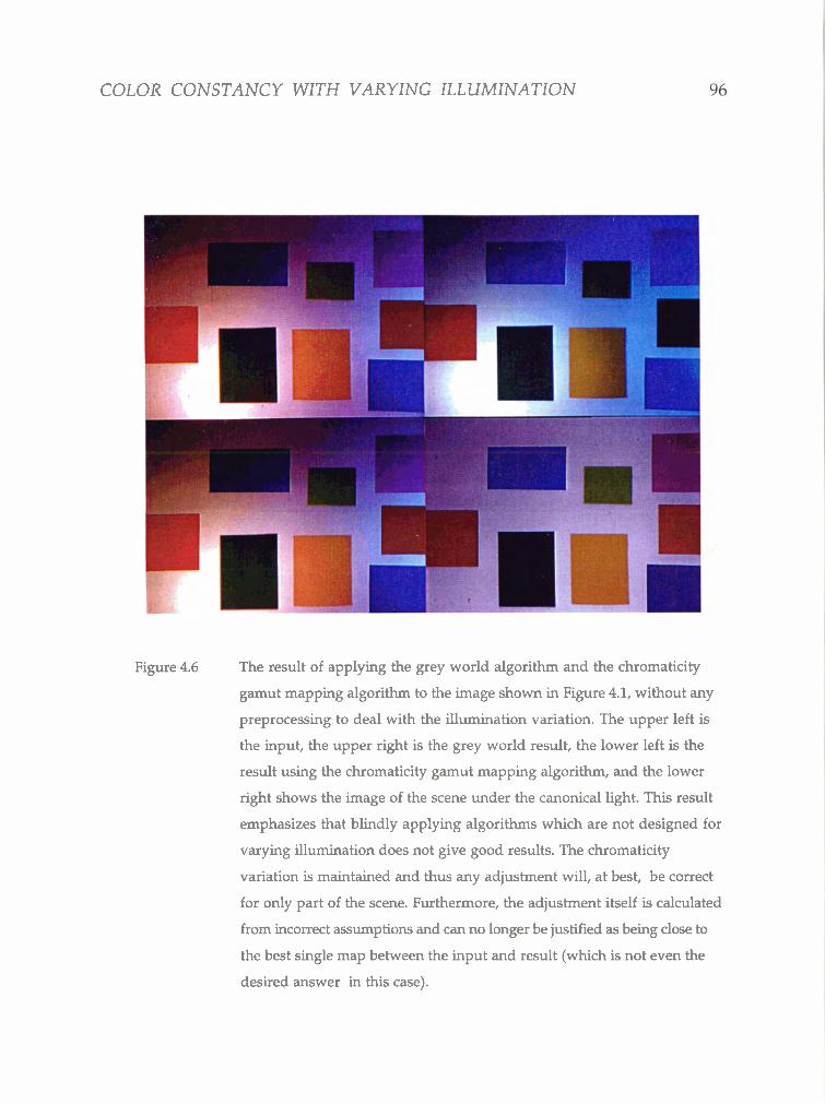
processing to remove the variation is still required. The result of blindly
COLOR CONSTANCY WITH VARYING ILLUMINATION
applying the non-varying illumination algorithms to the image with varying
illumination is shown in Figure 4.6. Figure 4.7 shows the mapping
constraints for this image. It is clear that the varying illumination constraints
are very strong here, and alone would be sufficient to give a good answer.
Figure 4.1 Image of a wall with colored paper illuminated on the left by
incandescent light, and on the right by simulated daylight.
COLOR CONSTANCY WITH VARYING ILLUMINATION
Figure 4.2 The results of segmenting the image shown in Figure 4.1, with all points
contributing to the equations used to solve for the varying illumination
map shown in red.
COLOR CONSTANCY WITH VARYING ILLUMINATION
Figure 4.3 The results of removing the illumination chromaticity variation from the
image shown in Figure 4.1. The image is adjusted so that the estimated
chromaticity of the light is the same as that for the center of the original
image.
COLOR CONSTANCY WITH VARYING ILLUMINATION
Figure 4.4 The illumination chromaticity variation map for the image shown in
Figure 4.1.
COLOR CONSTANCY WITH VARYING ILLUMINATION
Figure 4.5 The result of color constancy processing for the image shown in Figure 4.1,
and reproduced in the upper left. The upper right is the result of applying
surface and illumination constraints to the image with illumination color
variation removed (see Figure 4.3). The lower left is the result of including
the varying illumination constraints. It is very much the same due to the
fortuitous selection of paper colors. The desired colors are shown in the
lower right, which is the same scene taken under the Philips CW
fluorescent light used as the canonical. It should be pointed out that
illumination intensity could be dealt with by the methods used for
chromaticities, but for these experiments only chromaticity was corrected
for. Hence the algorithm results show variation in intensity which is not
present in the target image.
COLOR CONSTANCY WITH VARYING 1LLUMlNATlON
Figure 4.6 The result of applying the grey world algorithm and the chromaticity
gamut mapping algorithm to the image shown in Figure 4.1, without any
preprocessing to deal with the illumination variation. The upper left is
the input, the upper right is the grey world result, the lower left is the
result using the chromaticity gamut mapping algorithm, and the lower
right shows the image of the scene under the canonical light. This result
emphasizes that blindly applying algorithms which are not designed for
varying illumination does not give good results. The chromaticity
variation is maintained and thus any adjustment will, at best, be correct
for only part of the scene. Furthermore, the adjustment itself is calculated
from incorrect assumptions and can no longer be justified as being close to
the best single map between the input and result (which is not even the
desired answer in this case).
COLOR CONSTANCY WITH VARYING ILLUMINATION
I
IConstraint - Intersection of V Constraint(s) ---- Intersection of S Constraint(~) - --.-
Best 2D D-Ma o HUU ~ v e , g +
Hull Ave, S and I Hull Ave, S, I, and V x
1 2 3 4 5 6 7 First Componant of Diagonal Transform
Figure 4.7 The constraints on the mappings to the canonical illurninant determined from
the image with the illumination color removed, and including the varying
illumination constraints. Note that the best fit (Best 2D D-Map) is for mapping
the image with the illumination chromaticity removed to the image taken
with the canonical light.
COLOR CONSTANCY WITH VARYING ILLUMINATION
a c 8 0.~2 0 0 0.2 First Componant 0.4 of Diagonal 0.6 Transform 0.8 1
Two Dimensional Diagonal Gamut Mappings
Figure 4.8 Figure 4.7 magnified to show the intersections in more detail.
1.2
6 I 1 r= - I 0.8
* 0
0.6
g s 0.4
I
I Constraint - -
- Hull Ave, S, I, and V x
____-----
- -
-
_ _ _ _ _ - - - - - - _ _ _ . - I - - - -
COLOR CONSTANCY WITH VARYING ILLUMINATION
The image analyzed in the preceding text had enough fortuitous colors
that once the variation in the illumination chromaticity was removed,
excellent color constancy was possible even without using the illumination
variation. However, illumination variation can constrain the desired
solution even when there are few colors in the scene. Figure 4.9 shows the
results obtained by applying the algorithm to an image of a single green card
taken under similar circumstances to the previous image. Figure 4.10 shows
the constraints obtained, and it is clear that the varying illumination alone
provides a significant restrictions on the possible mappings.
The varying illumination was also tested on the Mondrian image
illuminated under similar conditions to the previous two images. The results
are shown in Figure 4.11. Again, the results are good, and indicate that this is
a very promising method.
COLOR CONSTANCY WITH VARYING ILLUMINATION
Figure 4.9 The results of the comprehensive algorithm applied to a single green card
illuminated on the left by a regular incandescent light, and on the right by
simulated blue sky. The upper left is the input. The upper right is the result of
blindly using the grey world algorithm. The lower left is the result of using the
varying illumination algorithm described in this chapter. The lower right is
the image taken under the canonical illuminant (Phillips CW fluorescent).
COLOR CONSTANCY WITH VARYING ILLUMINATION
T
I I I L
5 10 15 20 First Componant of Diagonal Transform
Two Dimensional Diagonal Gamut Mappings I I 1
I Constraint - Intersection of V Constraint(s)
..................... Intersection of S Constraint(~) - - - - - Best 2DDMap o
Gre World + I - I u i ~ v e , ~
Hull Ave, S and I x Hull Ave, S, I, and V A
X
0
Figure 4.10 The constraints on the illumination mappings for the image shown in Figure 4.9.
As one would expect, the single surface constraint does not help much. However,
the varying illumination yields a reasonable solution. It should be noted that
the best fit shown on the plot is the best fit between the image with the
illumination chromaticity variation removed and the image under the
canonical illuminant.
COLOR CONSTANCY WITH VARYING ILLUMINATION
Figure 4.11 The results of the comprehensive algorithm applied to the Mondrian
illuminated on the left by a regular incandescent light, and on the right by
simulated blue sky. The upper left is the input. The upper right is the result of
using the illumination and surface constraints on the image with the
illumination chromaticity removed. The lower left is the result of using the
illumination variation constraints as well. Again, in the case of sufficient color,
it does not make much difference. The obviously incorrect region on the middle
right of these two images is due to insufficient information to solve for the
variation in illumination due saturation in the original image. This problem
could be dealt with. The lower right is the image taken under the canonical
illuminant (Phillips CW fluorescent).
Conclusion
The goal of this work was to investigate the application of color
constancy algorithms to image data. This proved to be possible in the case of
chromatically uniform illumination under arbitrary conditions. In addition,
it was possible to extend the results of a recent algorithm for color constancy
under varying illumination so that it worked very well in the case of simple
images.
The journey began with a series of measurements to explore the nature
of the lights, surfaces, and camera sensors which contribute to the images that
need to be analyzed. It was found that published data was not sufficient to
cover the surfaces in our laboratory. Specifically, success with the book scene
presented in chapter 3 required adding measured data to the canonical gamut.
An additional contribution was a simple implementation of a camera
calibration technique based on that of Vhrel and Trussel [VT92].
Then some current ideas in color constancy were investigated. First,
sensor sharpening was considered as a method for improving the
performance of the algorithms. Here it proved difficult to identify a
CONCLUSIONS 104
sharpening transform for a wide range of illuminants which unambiguously
improved the algorithms. The search was made difficult by the complicating
factor that the negative sensor values that may be produced by sharpening can
lead to problems with the gamut mapping algorithms. It seems that insisting
on the best solution for all algorithms with all illuminants (as is the case with
overall optimization proposed in s3.2) leads to poor performance for some of
the algorithms under the test illuminants. Thus it is suggested that sensor
sharpening must be further investigated with respect to specific algorithms in
the context of a wider illumination set.
Fortunately the problems found with sharpening can be ignored
because the camera sensors are already quite sharp (as verified in Table 3.1).
Working with unmodified sensors, a number of color constancy algorithms
were tested on generated data. It was found that the gamut mapping approach
performed better than more naive methods, but it was necessary to include
the illumination constraint proposed by Finlayson [Fin95]. Furthermore,
using the hull average as suggested in this work, as opposed to the
maximum-volume-mapping heuristic used previously, increased the
number of cases where the gamut mapping algorithms performed better.
Although the results were not completely unanimous, given its relative
efficacy, combined with the esthetics of constraining rather than guessing a
solution, the gamut mapping approach is the current method of choice. This
is heavily supported by the results of the experiments on image data. In these
experiments, the grey world algorithm was preferred only once out of 12
combinations of unknown illuminant and image scene.
CONCLUSIONS
In the final leg of the journey, a different challenge for color constancy
research was confronted, namely dealing with scenes with varying
illumination. First a very promising algorithm [FFB95] was modified so that
it could be used as part of a comprehensive color constancy algorithm. Then
experiments on generated data verified that all three classes of constraints,
specifically those due to surfaces, illumination, and varying illumination,
worked together to give better color constancy. At this point, we were still
without a method for identifying the varying illumination, and thus a robust
method for doing this was proposed. This method requires segmenting the
image, which is a difficult problem especially if the illumination may vary.
Nonetheless, simple images were successfully segmented by region growing
using small jumps in both chromaticity and RGB as the condition for
inclusion into a region. This segmentation method allowed the
comprehensive color constancy algorithm to be tested on image data, and the
results were excellent.
Thus to a reasonable extent, the original goal has been achieved. It is
worth pointing out that no color constancy processing on real image data
with a non-negligible amount of varying illumination has been reported in
the literature. Along similar lines, even for the common assumption of
uniform illumination, results in the literature for image data are very sparse.
Certainly there are no published results for color constancy processing on
images as general as our book scenes. Hence the work in this thesis
significantly extends the quality and quantity of practical color constancy
results.
Appendix A
Selecting Solutions by Centroid
In this work the preferred method to select solutions was to use the
centroid of the solution set. Intuitively, this is a good choice, but it can also be
justified formally without too much effort. To do this, we make two simple
assumptions. First, we assume that all candidate solutions are equally likely
Second, we accept the definition of the error to be the vector magnitude
difference between the estimate and the actual value.
The assumption that all candidate solutions are equally likely means
that the probability density function, P(X), is a constant over the solution set:
P(X)=C ( A 4
Although the value of C is not required, it is easily specified. Since we must
have:
P ( X ) dv = 1 Solution Set
C is given by:
APPENDIX A
Now suppose that X* is a proposed solution. Given that all solutions
are equally likely, the expected value of the error squared is given by:
2
E 2 = 1 C 11 x * -x 11 dv Solution
(A.3) Set
Working with the components we have:
Set
Now consider varying X* to minimize the error. To minimize the error, we
can minimize the error squared. To find the best value of X* we set the
partial derivative with respect to each component to zero. Using "I" to
designate a specific choice of component:
2 4 j C x (x i -x ; ) dv = 0 ax1 solution i
Set
j(x, - x,*) dv = 0 Solution Set
jx , dv = jx,* dv Solution Solution Set Set
(Ignoring a factor of -2C)
APPENDIX A
X I * I d v = I x , d v Solution Solution Set Set
Finally, for each component x,* of the minimum error solution we get:
solition Set x,* =
Solution Set
This final equation defines the components of the centroid, and so we are
done.
Bibliography
D.H. Brainard and W.T. Freeman, "Bayesian method for recovering surface and illuminant properties from photosensor responses", Human Vision, Visual Processing, and Digital Display V, pp. 364-376, (1994)
G. Buchsbaum, "A spatial processor model for object colour perception", Journal of the Franklin Institute, 310, pp. 1-26, (1980)
M.H. Brill and G. West, "Contributions to the Theory of Invariance of Color Under the Condition of Varying Illumination", Journal of Mathematical Biology, 11, pp, 337-350, 1981
J. Cohen, "Dependency of The Spectral Reflectance Curves of The Munsell Color Chips", Psychon. Sci., 1, pp. 369-370, (1964)
E.R. Dixon, "Spectral distribution of Australian daylight", Journal of the Optical Society of America, 68, pp. 437-450, (1978)
W. Freeman and David Brainard, "Baysian Desion Theory, the Maximum Local Mass Estimate, and Color Constancy", in Proceedings: Fifth International Conference on Computer Vision, pp 210-21 7, (IEEE Computer Society Press, 1995)
BIBLIOGRAPHY 110
B. V. Funt, M. S. Drew, M. Brockington, "Recovering Shading from Color Images", in Proceedings: Second European Conference on Computer Vision, G.Sandini, ed., 1992.
G.D. Finlayson and M.S. Drew and B.V. Funt, "Spectral Sharpening: Sensor Transformations for Improved Color Constancy", Journal of the Optical Society of America A, 11, 5, pp. 1553-1563, (1994)
G.D. Finlayson and M.S. Drew and B.V. Funt, "Color Constancy: Generalized Diagonal Transforms Suffice", Journal of the Optical Society of America A, 11, pp. 3011-3020, (1994)
G.D. Finlayson and B.V. Funt, "Color Constancy with Shadows", Perception, 23, (Special issue on the 17th European Conference on Visual Perception, Eindhoven), pp. 89-90, (1994)
G. D. Finlayson, B. V. Funt, and K. Barnard, "Color Constancy Under Varying Illumination", in Proceedings: Fifth International Conference on Computer Vision, pp 720-725, 1995.
G.D. Finlayson, "Color Constancy and a Changing Illumination", In Human Vision, Visual Processing, and Digital Display V, pp. 353-363, (1994)
G. D. Finlayson, "Color Constancy in Diagonal Chromaticity Space", in Proceedings: Fifth International Conference on Computer Vision, pp 218-223, (IEEE Computer Society Press, 1995).
D. Forsyth, "A novel algorithm for color constancy", Int. J. Computer. Vision, 5, pp. 5-36, (1990)
R. Gershon and A.D. Jepson and J.K. Tsotsos, "Ambient illumination and the determination of material changes", Journal of the Optical Society of America A, 3, pp. 1700-1707, (1986)
R. C. Gonzalez and P. Wintz, Digital Image Processing, Second Edition, (Addison-Wesley 1987)
B.K.P. Horn, "Determining lightness from an image, Computer Vision, Graphics, and Image Processing, 3, pp. 277-299, (1974)
BIBLIOGRAPHY 111
D.B. Judd and D.L. MacAdam and G. Wyszecki, "Spectral Distribution of Typical Daylight as a Function of Correlated Color Temperature", Journal of the Optical Society of America, 54, pp. 1031-1040, (August 1964)
E.L. Krinov, "Spectral Reflectance Properties of Natural Formations", Technical Translation TT-439, National Research Council of Canada, (1947)
E.H. Land, "The Retinex theory of Color Vision", Scientific American, 108-129, (1977)
E.H. Land, "Recent advances in Retinex theory", Vision Res., 26, pp. 7-21, (1986)
E. H. Land and J. J. McCann, "Lightness and Retinex Theory", Journal of the Optical Society of America, 61, 1, pp. 1-11, (1971).
John J. McCann, Suzanne P. McKee, and Thomas H. Taylor, "Quantitative Studies in Retinex Theory", Vision Research, 16, pp. 445-458, (1976)
L.T. Maloney and B.A. Wandell, "Color constancy: a method for recovering surface spectral reflectance", Journal of the Optical Society of America A, 3, pp. 29-33, (1986)
D.H. Marimont and B.A. Wandell, "Linear models of surface and illuminant spectra", Journal of the Optical Society of America A, 9, 11, pp. 1905-1913, (1992)
D. Nickerson, Spectrophotometric Data for a Collection of Munsell Samples, U.S. Department of Agriculture. Wahsington D.C., (1957)
J. P. S. Parkkinen and J. Hallikanen and T. Jaaskelainen, "Characteristic spectra of Munsell Colors", Journal of the Optical Society of America A, 6, pp. 318-322, (1989)
S.A. Shafer, "Using color to separate reflection components", Color Res. Appl., 10, pp. 210-218, (1985)
BIBLIOGRAPHY 112
G. Sharma and H.J. Trussel, "Characterization of Scanner Sensitivity", In IS6T and SID's Color Imaging Conference: Transforms 6 Transportability of Color, pp. 103-107, (1993)
M. Tsukada and Y. Ohta, "An Approach to Color Constancy Using Multiple Images", in Proceedings Third International Conference on Computer Vision, (IEEE Computer Society, 1990)
S. Tominaga, "Realization of Color Constancy Using the Dichromatic Reflection Model", in The second IS6T and SID's Color Imaging Conference, pp. 37-40, (1994)
M.J. Vrhel and H.J. Trussel, "Physical Device Illumination Correction", in Device-Independent Color Imaging and Imaging Systems Integration, Vol. 1909, pp. 84-91, (1993),
B.A. Wandell, "The synthesis and analysis of color images", IEEE Trans. Putt. Anal. and Mach. Intell., 9, pp. 2-13, (1987)
G. West and M.H. Brill, "Necessary and sufficient conditions for von Kries chromatic adaption to give colour constancy", J. Math. Biol., 15, pp. 249-258, (1982)
G. Wyszecki and W.S. Stiles, Color Science: Concepts and Methods, Quantitative Data and Formulas, 2nd edition, (Wiley, New York, 1982)
M. D'Zmura and G. Iverson, "Color constancy. I. Basic theory of two-stage linear recovery of spectral descriptions for lights and surfaces", Journal of the Optical Society of America A, 10, pp. 2148-2165, (1993)