Computational Fluid Dynamic (CFD) Analysis of a Generic Missile With Grid Fins by James DeSpirito, Harris L. Edge,Paul Weinacht, Jubaraj Sahu, and Surya Dinavahi ARL,-‘R-23 18 L . September 2000 Approved for public release; distribution is unlimited.
Transcript
Computational Fluid Dynamic (CFD) Analysis of a Generic Missile
With Grid Fins
by James DeSpirito, Harris L. Edge, Paul Weinacht, Jubaraj Sahu, and Surya Dinavahi
ARL,-‘R-23 18
L
.
September 2000
Approved for public release; distribution is unlimited.
The findings in this report are not to be construed as an official Department of the Army position unless so designated by other authorized documents.
Citation of manufacturer’s or tradenames does not constitute an official endorsement or approval of the use thereof.
Destroy this report when it is no longer needed. Do not return it to the originator.
I
,
Abstract
ii
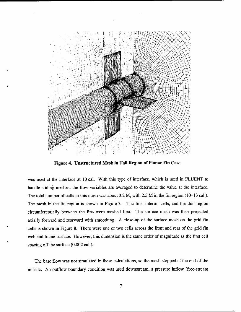
This report presents the results of a study demonstrating an approach for using viscous computational fluid dynamic simulations to calculate the flow field and aerodynamic coefficients for a missile with grid fins. A grid fm is an unconventional lifting and control surface that consists of an outer frame supporting an inner grid of intersecting planar surfaces of small chord. The calculations were made at a Mach number of 2.5 and several angles of attack for a missile without fins, with planar fins, and with grid fins. The results were validated by comparing the computed aerodynamic coefficients for the missile and individual grid fins against wind tunnel measurement data. Very good agreement with the measured data was observed for all configurations investigated. For the grid fm case, the aerodynamic coefficients were within 2.8- 6.5% of the wind tunnel data. The normal force coefficients on the individual grid fins were within 11% of the test data. The simulations were also successful in calculating the flow structure around the fin in the separated-flow region at the higher angles of attack. This was evident in the successful calculation of the nonlinear behavior for that fin, which showed negative normal force at the higher angles of attack. The effective angle of attack is negative on either part of or all of the top grid fm for the higher angles of attack.
L
Acknowledgments
The authors would like to thank Graham Simpson and Anthony Sadler of the Defence
Evaluation and Research Agency, United Kingdom, for providing the comprehensive database of
wind tunnel test data. Thanks are also due to support engineers at Fluent, Inc., for insight on
approaches for mesh generation of the grid fm configuration.
This work was supported in part by a grant of high performance computing time from the
Department of Defense High Performance Computing Center at Aberdeen Proving Ground,
3.1 Aerodynamic Coefficients ................................................................................... 11 3.1.1 Body Alone Case (BIA) ................................................................................. 11 3.1.2 Planar Fin Case (BlAC2R) ........................................................................... 12 3.1.3 Grid Fin Case (BIAL2R) ............................................................................... 15 3.1.4 Forces on Fins ............................................................................................... 18 3.2 Grid Fin Flow Field ............................................................................................. 20
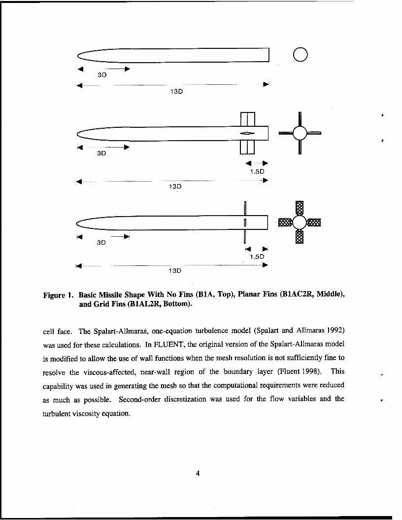
1. Basic Missile Shape With No Fins (BlA, Top), Planar Fins (BlAC2R, Middle), and Grid Fins (B lAL2R, Bottom) .............................................................................
Unstructured Mesh for Basic Missile Shape Without Fins .......................................
Unstructured Mesh for Basic Missile Shape With Planar Fins .................................
Unstructured Mesh in Tail Region of Planar Fin Case ..............................................
Geometry for Grid Fin Case (B lAL2R) ....................................................................
Unstructured Mesh for Basic Missile Shape With Grid Fins ....................................
Unstructured Mesh in Tail Region of Grid Fin Case .................................................
Surface Mesh on Grid Fin Cells ................................................................................
Axes and Sign Convention for Force and Moment Coefficients ...............................
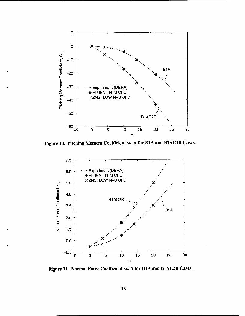
Pitching Moment Coefficient vs. a for B 1 A and B 1 AC2R Cases ............................
Normal Force Coefficient vs. a for B 1A and B lAC2R Cases ..................................
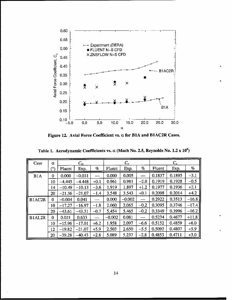
Axial Force Coefficient vs. a for BlA and B lAC2R Cases .....................................
Pitching Moment Coefficient vs. a for B lAL2R Case .............................................
Normal Force Coefficient vs. a for B lAL2R Case ...................................................
Axial Force Coefficient vs. a for B 1 AL2R Case ......................................................
Normal Force Coefficient on Individual Grid Fins vs. a ..........................................
Mach Contours on Symmetry Plane for Grid Fin Case, a = 10” ..............................
Mach Contours on Symmetry Plane for Grid Fin Case, a = 20” ..............................
Pressure Coefficient Contours on Symmetry Plane Through Bottom Fin (Fin 2) ....
vii
4
6
6
7
8
8
9
9
12
13
13
14
16
16
17
19
20
21
22
Figure
20.
21.
Pressure Coefficient Contours on Symmetry Plane Through Top Fin (Fin 4) . . . . . . . . . .
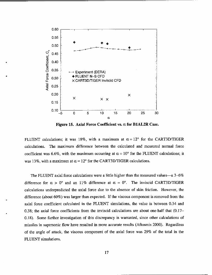
Figure 15. Axial Force Coefficient vs. a for BlAL2R Case.
FLUENT calculations; it was 18%, with a maximum at a = 12” for the CART3D/TIGER
calculations. The maximum difference between the calculated and measured normal force
coefficient was 6.6%, with the maximum occurring at a = 10” for the FLUENT calculations; it
was 13%, with a maximum at a = 12” for the CART3D/TIGER calculations.
The FLUENT axial force calculations were a little higher than the measured values-a 3-6%
difference for a > 0” and an 11% difference at a = 0”. The inviscid CART3D/TIGER
calculations underpredicted the axial force due to the absence of skin friction. However, the
difference (about 60%) was larger than expected. If the viscous component is removed from the
axial force coefficient calculated in the FLUENT simulations, the value is between 0.34 and
0.38; the axial force coefficients from the inviscid calculations are about one-half that (0.17-
0.18). Some further investigation of this discrepancy is warranted, since other calculations of
missiles in supersonic flow have resulted in more accurate results (Aftosmis 2000). Regardless
of the angle of attack, the viscous component of the axial force was 29% of the total in the
FLUENT simulations.
17
The inviscid calculations show that the total normal force and pitching moment data can be
predicted to within 18% of the experimental data. If accurate axial force or drag information is
not required, then the inviscid calculations may provide the information needed to check out
multiple design approaches. Whether using CART3D/TIGER or an inviscid solution with
FLUENT, the reduction in computing time is substantial.
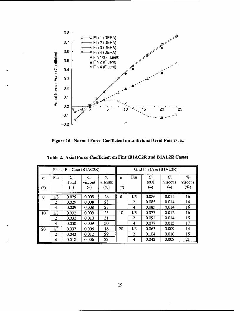
3.1.4 Forces on Fins. The normal force coefficients on the individual grid fins from the
FLUENT calculations are shown in Figure 16, along with the measured wind tunnel data
(Simpson 1997) as a function of a. The fins are numbered 1-4, with fin 1 in the 3 o’clock
position and fm 4 in the 12 o’clock position if looking forward from the rear of the missile in the
“+” configuration. In the simulations, fins 1 and 3 are the same due to symmetry. The normal
force on the fins was predicted very well, with the largest difference at about 11%. As expected,
the normal force is greatest on the horizontal fins. The windward fin (fin 2, bottom) also
provides a substantial normal force. The leeward fm (fin 4, top) provides a similar normal force
as fin 2 up to about a 4” angle of attack, but then goes nonlinear and negative at higher angles of
attack. As described by Simpson (1997), the nonlinear shape of the normal force vs. a curve for
the leeward fm is caused by its location in the separated flow region at higher angles of attack.
As shown later in plots of the flow field, the local angle of attack varies over the leeward grid
fin. Some parts of the fin will be at an effective negative angle of attack, while other parts are at
an effective positive angle of attack.
.
The axial force coefficients on individual grid fins were about 2-3 times greater than those
on the planar fins. The viscous component of the axial force on the grid fm was about 1.5 times
greater than on the planar fin. These values are presented in Table 2. Although it was
speculated that the smaller chord of the grid fm might impart fewer viscous effects than a planar
fin (Sun and Khalid 1998), the summation of the viscous effects of all the lattice surfaces of the
grid fm leads to higher viscous forces. The likely reason inviscid calculations of the
aerodynamic coefficients on a missile with grid fins were more accurate than those for a missile
with planar fins (Sun and Khalid 1998) is that the viscous component, as a percentage of the total
18
0.8
0.7
0.6
0.5
0.4
0.3
0.2
0.1
0.0
-0.1
-0.2
M Fin 1 (DERA) M Fin 2 (DERA) +-o Fin 3 (DERA) w Fin 4 (DERA)
+ Fin l/3 (Fluent) A Fin 2 (Fluent) V Fin 4 (Fluent)
Figure 16. Normal Force Coeffkient on Individual Grid Fins vs. a.
Table 2. Axial Force Coefficient on Fins (BlAC2R and BlAL2R Cases)
19
t
1.63e+OO
t 1.36e+OO
i l.O9e+OO
8.15e-01
I 543e-01
2.72e-01 L X
O.OOe+OO
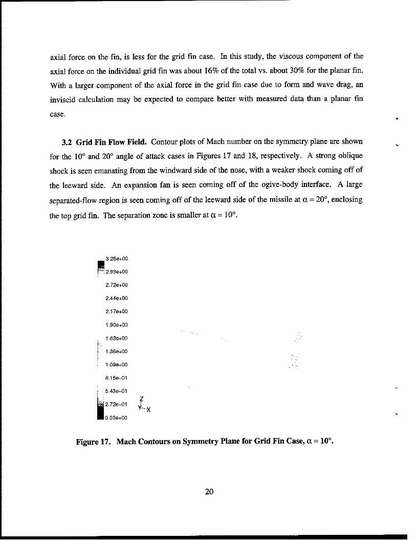
Figure 17. Mach Contours on Symmetry Plane for Grid Fin Case, a = 10”.
20
axial force on the fin, is less for the grid fm case. In this study, the viscous component of the
axial force on the individual grid fm was about 16% of the total vs. about 30% for the planar fin.
With a larger component of the axial force in the grid fin case due to form and wave drag, an
inviscid calculation may be expected to compare better with measured data than a planar fm
case.
3.2 Grid Fin Flow Field. Contour plots of Mach number on the symmetry plane are shown
for the 10” and 20” angle of attack cases in Figures 17 and 18, respectively. A strong oblique
shock is seen emanating from the windward side of the nose, with a weaker shock coming off of
the leeward side. An expansion fan is seen coming off of the ogive-body interface. A large
separated-flow region is seen coming off of the leeward side of the missile at a = 20”, enclosing
the top grid fin. The separation zone is smaller at a = 10”.
3.26e+OO
2.99e+OO
2.72e+OO
2.44e+OO
2.17e+OO
1.90e+OO
3.00e+oo
2.67ecOO
2.33e+OO
2.00e+oo
I i; 1.67e+OO
1.330+00
1 .ooe+oo
6.67e-01
3.33e-01 45 X
O.OOe+OO
Figure 18. Mach Contours on Symmetry Plane for Grid Fin Case, a = 20”.
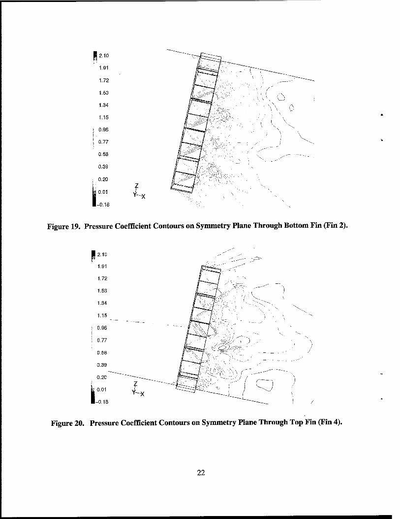
There is a complex, three-dimensional shock structure emanating off of the grid fins.
Figures 19 and 20 show pressure contours on the symmetry plane through the bottom and top
fins, respectively, at a = 12”. The outline of the grid fin frame is shown in the figures, with the
shocks emanating off of the intersection of several grid fm cells (see Figures 7 and 8). At this
Mach number, the shock and expansion waves do not reflect off of the interior walls of the grid
fm cells (Washington and Miller 1998). Instead, they first reflect off of one another inside the
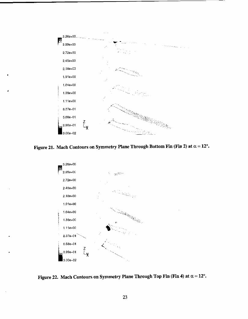
grid fin cell, setting up several more reflections in the wake of the fin. In Figures 21 and 22,
contours of Mach number are shown on the bottom and top fins for a = 12”. For the bottom fm
(Figure 21), the entire fin is at a positive relative angle of attack so that there is an expansion fan
emanating from the lower part of each cell and a shock wave emanating off of the upper part of
each cell. Part of the top fm (Figure 22) is at a negative relative angle of attack with respect to
the incident flow; this is due to the vortices in the separation zone on the leeward side of the
missile. The top cell is at a positive angle of attack, with the shock wave emanating from the top
of the cell. The cell second from the top is nearly at a 0” angle of attack, with shock waves
21
R 2.10 i
1.91
1.72
1.53
1.34
1.15
j 0.96
; 0.77
0.58
! 0.20
0.01
-0.18
L X
-A : : ‘\: “,
1
,, ‘..:. ‘,. ,, ; :, ;:.; ,‘, :
i ;:
-_ ‘;,:,.;T 8, I , :.,’ .’
.::’ ,.; _\ ,.. t, .-.: ‘, \. ‘\. \ iJ I
Figure 19. Pressure Coefficient Contours on Symmetry Plane Through Bottom Fin (Fin 2).
a 2.10 _'
1.91
1.72
1.53
I 0.96
0.58
Figure 20. Pressure Coefficient Contours on Symmetry Plane Through Top Fin (Fin 4).
22
.
3.26e+00. --. . I,, .,
I ,. 2,72e+OO 0
2.45e+OO
2.1&3+00
1.91e+OO
t 1.64e+OO
! 1,38e+OO
1.11e+OO
2.99e-01
3,00e-02
b. . ”
“ , I , , , “’ “ ,
: _:
Figure 21. Mach Contours on Symmetry Plane Through Bottom Fin (Fin 2) at a = 12’.
3.268+00
2,99e+OO
2,72e+OO
._ ,.- :. * ;-
2,45e+OO
2.18e+OO
1.910+00
1.64e+OO
! i 1,38e+OO / : l.lle+OO
8,37e-01 \'~'y,~
; 568e-01
2.99e-01
3.00e-02
Figure 22. Mach Contours on Symmetry Plane Through Top Fin (Fin 4) at a = 12”.
23
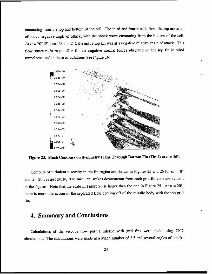
emanating from the top and bottom of the cell. The third and fourth cells from the top are at an
effective negative angle of attack, with the shock wave emanating from the bottom of the cell.
At a = 20” (Figures 23 and 24), the entire top fm was at a negative relative angle of attack. This
flow structure is responsible for the negative normal forces observed on the top fm in wind
tunnel tests and in these calculations (see Figure 16).
3.98e+OO ‘.-
3,32e+OO‘
2.990+00
2.66e+OO
2.33e+OO
2.00e+oo
1"..'1.67e+OO 1
1.34e+OO
l.O2e+OO
[ .6.85&01
3.568-01
2.57e-02
.
Figure 23. Mach Contours on Symmetry Plane Through Bottom Fin (Fin 2) at a = 20°.
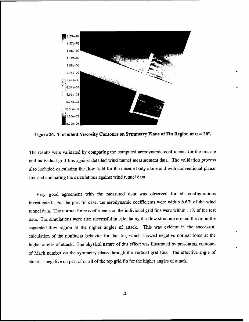
Contours of turbulent viscosity in the fm region are shown in Figures 25 and 26 for a = 10”
and a = 20”, respectively. The turbulent wakes downstream from each grid fm vane are evident
in the figures. Note that the scale in Figure 26 is larger than the one in Figure 25. At a = 20”,
there is more interaction of the separated flow coming off of the missile body with the top grid
fin.
4. Summary and Conclusions
Calculations of the viscous flow past a missile with grid fins were made using CFD
simulations. The calculations were made at a Mach number of 2.5 and several angles of attack.
24
3.98e+OO
3.651~00 "'̂ ,.
3.328+00 '> 'i
.,
, '2 2.990+00
:..w '$C
2.66e+OO
2,33e+OO
1; 2.00e+oo ‘L,
t
'., -*i
l 1.67e+OO Y..
-.._ . . . .
/ ~ 1.34e+OO
1.02e+OO
j 6.85e-01
3.56e-01 k
2.57e-02
‘.
Figure 24. Mach Contours on Symmetry Plane Through Top Fin (Fin 4) at a = 20”.
4.80e-03
4.40e-03
4.00e-03
3,60e-03
3.20e-03
2.80e-03
2.40e-03
1: 2.00e-0:
! 1,60e-0,
1.20e-0,
i 8.00e-0
Figure 25. Turbulent Viscosity Contours on Symmetry Plane of Fin Region at a = 10”.
1.37~~02'
1.25e-02
1.12e-02 h
9.98e-03
8.74e-03 k
1: j 7.49e-03
f+.j 6.24e-03 [ i
I 4.990-03
3.74e-03
! 2.50e-03
1.25e-03
O.OOe+OO
Figure 26. Turbulent Viscosity Contours on Symmetry Plane of Fin Region at a = 20”.
The results were validated by comparing the computed aerodynamic coefficients for the missile
and individual grid fins against detailed wind tunnel measurement data. The validation process
also included calculating the flow field for the missile body alone and with conventional planar
fins and comparing the calculations against wind tunnel data.
Very good agreement with the measured data was observed for all configurations
investigated. For the grid fin case, the aerodynamic coefficients were within 6.6% of the wind
tunnel data. The normal force coefficients on the individual grid fins were within 11% of the test
data. The simulations were also successful in calculating the flow structure around the fin in the
separated-flow region at the higher angles of attack. This was evident in the successful
calculation of the nonlinear behavior for that fin, which showed negative normal force at the
higher angles of attack. The physical nature of this effect was illustrated by presenting contours
of Mach number on the symmetry plane through the vertical grid fins. The effective angle of
attack is negative on part of or all of the top grid fin for the higher angles of attack.
26
The viscous component of the axial force on the grid fin was about 1.5 times greater than that
on the planar fin. This contrasts previous speculation that the smaller chord of the grid fin would
result in less viscous force than a planar fin. The total axial force on grid fin was about 2-3
times greater than that on the planar fin. As a percentage of the total force, the viscous
component was about 16% for the grid fin and about 30% for the planar fin.
Results for inviscid calculations of the grid fin case were also presented. The normal force
and pitching moment coefficients were calculated to within 18% of the experimental data. If
axial force or drag information is not required, then inviscid calculations may provide reasonable
design data in less time than viscous calculations.
The investigation detailed in this report demonstrated an approach for using viscous CFD
simulations to calculate the flow field and aerodynamic coefficients for a missile with grid fins.
Nevertheless, even when an unstructured mesh and wall functions were used to reduce the mesh
size and computational requirements, substantial computing resources were required. An
alternative approach would be to use the chimera overset grid technique to generate a structured
mesh; however, the nature of the grid fm design makes the required resources large, regardless
of the approach used. Inviscid calculations showed that the normal force and pitching moment
coefficients could be calculated with reasonable accuracy.
27
.
I~E~I~NALLY Lwr BLANK.
28
5. References
Abate, G., R. P. Duckerschein, and W. Hathaway. “Subsonic/Transonic Free-Flight Tests of a Generic Missile with Grid Fins.” AIAA Paper 2000-0937, January 2000.
Abate, G., R. P. Duckerschein, and G. Winchenbach. “Free-Flight Testing of Missiles with Grid Fins.” Proceedings of the 50th Aeroballistic Range Association Meeting, Pleasanton, CA, November 1999.
Aftosmis, M. J., Personal communication. NASA Ames Research Center, Moffett Field, CA, January 2000.
Aftosmis, M. J., M. J. Berger, and J. E. Melton. “Robust and Efficient Cartesian Mesh Generation for Component-Based Geometry.” AZAA Journal, vol. 36, no. 6, pp. 952-960, 1998.
Aftosmis, M. J. “Solution Adaptive Cartesian Grid Methods for Aerodynamic Flows with Complex Geometries.” Computational Fluid Dynamics VKI Lectures Series 1997-05, von Karman Institute for Fluid Dynamics, Belgium, 1997.
Burkhalter, J. E. “Grid Fins for Missile Applications in Supersonic Flow.” AIAA Paper 96-0194, January 1996.
Burkhalter, J. E., and H. M. Frank. “Grid Fin Aerodynamics for Missile Applications in Subsonic Flow.” J. Spacecraft and Rockets, vol. 33, no. 1, pp. 38-44, 1996.
Burkhalter, J. E., R. J. Hartfield, and T. M. Leleux. “Nonlinear Aerodynamic Analysis of Grid Fin Configurations.” J. ofAircraft, vol. 32, no. 3, pp. 547-554, 1995.
Chen, S., M. Khalid, H. Xu, and F. Lesage. “A Comprehensive CFD Investigation of Grid Fins as Efficient Control Surface Devices.” AIAA Paper 2000-0987, January 2000.
Edge, H. L., J. Sahu, W. B. Sturek, D. M. Pressel, K. R. Heavey, P. Weinacht, C. K. Zoltani, C. J. Nietubicz, J. Clarke, M. Behr, and P. Collins. “Common High Performance Computing Software Support Initiative (CHSSI) Computational Fluid Dynamics (CFD)-6 Project Final Report: ARL Block-Structured Gridding Zonal Navier-Stokes Flow (ZNSFLOW) Solver Software.” U. S. Army Research Laboratory, ARL-TR-2084, Aberdeen Proving Ground, MD, February 2000.
Khalid, M., Y. Sun, and II. Xu. “Computation of Flows Past Grid Fin Missiles.” Proceedings of the NATO RTO-MP-5, Missile Aerodynamics, NATO Research and Technology Organization, November 1998.
Kretzschmar, R. W., and J. E. Burkhalter. “Aerodynamic Prediction Methodology for Grid Fins.” Proceedings of the NATO RTO-MP-5, Missile Aerodynamics, NATO Research and Technology Organization, November 1998.
Lesage, F. “Numerical Investigation of the Supersonic Flow Inside a Grid Fin Cell.” Proceedings of the 17*h International Symposium on Ballistics, vol. 1, American Defense Preparedness Association, Arlington, VA, pp. 209-216, 1998.
Melton, J. E. “Automated Three-Dimensional Cartesian Grid Generation and Euler Flow Solutions for Arbitrary Geometries.” Ph.D. dissertation, University of California Davis, June 1996.
Melton, J. E., M. J. Berger, M. J. Aftosmis, and M. D. Wong. “3-D Applications of a Cartesian Grid Euler Method.” AIAA Paper 950853, January 1995.
Miller, M. S., and W. D. Washington. “An Experimental Investigation of Grid Fin Drag Reduction Techniques.” AIAA Paper 94-1914-CP, June 1994.
Simpson, G. M., and A. J. Sadler. “Lattice Controls: A Comparison with Conventional, Planar Fins.” Proceedings of the NATO RTO-MP-5, Missile Aerodynamics, NATO Research and Technology Organization, November 1998.
Simpson, G. “A Preliminary Analysis of the DERA Lattice Controls Database.” Defense Research Agency, DERA/AS/HWA/WP97 196/ 1 .O, Famborough, UK, July 1997.
Spalart, P. R., and S. R. Allmaras. “A One-Equation Turbulence Model for Aerodynamic Flows.” AIAA Paper 92-0439, January 1992.
Steger, J. L., F. C. Dougherty, and J. A. Benek. “A Chimera Grid Scheme.” Advances in Grid Generation, edited by K. N. Ghia and U. Ghia, American Society of Mechanical Engineers, ASME FED-5, New York, June 1983.
Sun, Y., and M. Khalid. “A CFD Investigation of Grid Fin Missiles.” AIAA Paper 98-3571, July 1998.
Tong, Z., 2. Lu, and X. Shen. “Calculation and Analysis of Grid Fin Configurations.” Advances in Astronautical Sciences, AAS 95-647, 1996.
30
Washington, W. D., and M. S. Miller. “Experimental Investigations of Grid Fin Aerodynamics: A Synopsis of Nine Wind Tunnel and Three Flight Tests. ” Proceedings of the NATO RTO- MP-5, Missile Aerodynamics, NATO Research and Technology Organization, November 1998.
Washington, W. D., and M. S. Miller. “Grid Fins - A New Concept for Missile Stability and Control.” AIAA Paper 93-0035, January 1993.
31
,
I~ENTI~NALLY mm BLANK.
32
NO. OF NO. OF ORGANIZATION COPIES ORGANIZATION COPIES
2
1
1
DEFENSE TECHNICAL 1 INFORMATION CENTER DTIC DDA 8725 JOHN J KINGMAN RD STE 0944 FT BELVOIR VA 22060-62 18
HQDA DAMOFDT 400 ARMY PENTAGON WASHINGTON DC 203 104460
1
OSD OUSD(A&T)/ODDDR&E(R) RJTREW THE PENTAGON WASHINGTON DC 20301-7100
1
DPTY CG FOR RDA us ARMYMATERLEL CMD 3 AMCRDA 5001 EISENHOWER AVE ALEXANDRIA VA 22333-0001
JNST FOR ADVNCD TCHNLGY THE UNIV OF TEXAS AT AUSTIN 1 PO BOX 202797 AUSTJN TX 78720-2797
DARPA B KASPAR 3701 N FAIRFAX DR ARLINGTON VA 22203-1714
US MILITARY ACADEMY MATH SC1 CTR OF EXCELLENCE MADNMATH MAJ HUBER THAYERHALL WEST POINT NY 109%-1786
DIRECTOR US ARMY RESEARCH LAB AMSRL D DRSMJTH 2800 POWDER MILL RD ADELPHJ MD 20783-l 197
DIRECTOR US ARMY RESEARCH LAB AMSRL DD 2800 POWDER MILL RD ADELPHJ MD 20783-l 197
DIRECTOR US ARMY RESEARCH LAB AMSRL CI AI R (RECORDS MGMT) 2800 POWDER MILL RD ADELPHJ MD 20783-l 145
DIRECTOR US ARMY RESEARCH LAB AMSRL CI LL 2800 POWDER MILL RD ADELPHJ MD 20783-l 145
DIRECTOR US ARMY RESEARCH LAB AMSRL CI AP 2800 POWDER MILL RD ADELPHJ MD 20783-l 197
ABERDEEN PROVING GROUND
DIR USARL AMSRL CI LP (BLDG 305)
33
NO. OF COPIES ORGANIZATION
7 CDR US ARMY ARDEC AMSTE AET A R DEKLEINE CNG R BO’I-I’ICELLI H HUDGINS J GRAU SKAHN W KOENIG PICATJNNY ARSENAL NJ 07806-5001
1 CDR US ARMY ARDEC AMSTE CCH V P VALENTI PICATINNY ARSENAL NJ 07806-5001
1 CDR US ARMY ARDEC SFAE FAS SD M DEVJNE PICATINNY ARSENAL NJ 07806-5001
2 USAF WRIGHT AERONAUTICAL LABS AFWALFIMG DR J SHANG N E SCAGGS WPAFB OH 45433-6553
3 AIR FORCE ARMAMENT LAB AFATJ&XA SCKORN B SIMPSON D BELK EGLIN AFB FL 32542-5434
1 AFRUMNAV G ABATE 101 W EGLIN BLVD, STE 219 EGLJN AFB FL 32542
1 CDR NSWC CODE B40 DR W YANTA DAHLGREN VA 22448-5 100
1 CDR NSWC CODE 420 DR A WARDLAW INDIAN HEAD MD 20640-5035
1 CDR NSWC DR F MOORE DAHLGREN VA 22448
NO. OF COPIES ORGANIZATION
1 NAVAL AIR WARFARE CENTER D FJNDLAY MS 3 BLDG 2187 PATUXENT RIVER MD 20670
1 DEFENSE JNTELLJGENCE AGENCY MISSILE AND SPACE INT. CENTER MSA- 1 A NICHOLSON BLDG 4545 FOWLER ROAD REDSTONE ARSENAL AL 35898-5500
4 DIR NASA LANGLEY RESEARCH CENTER TECH LJBRARY D M BUSHNELL DR M J HEMSCH DR J SOUTH LANGLEY STATION HAMPTON VA 23665
2 DARPA DR P KEMMEY DR J RICHARDSON 3701 NORTH FAIRFAX DR ARLINGTON VA 22203-1714
8 DIR NASA AMES RESEARCH CENTER T 27B-1 L SCHIFF T 27B-1 T HOLST MS 237-2 D CHAUSSEE MS 269-l M RAI MS 200-6 P KUTLER MS 258 1 B MEAKIN MS T27B-2 M AFTOSMIS MS T27B-2 J MELTON MOFFETT FIELD CA 94035
1 DIR NASA LANGLEY RESEARCH CENTER MS 499 P BUNING HAMPTON VA 2368 1
2 USMA DEPT OF MECHANICS LTC A L DULL M COSTELLO WEST POINT NY 10996
NO. OF COPIES ORGANIZATION
5 CDR USAAMCOM AMSAM RD SS AT E KREEGER G LANDINGHAM C D MIKKELSON E VAUGHN W D WASHINGTON REDSTONE ARSENAL AL 35898-5252
1 COMMANDER US ARMY TACOM-ARDEC BLDG 162s AMCPM DS MO PJBURKE PICATINNY ARSENAL NJ 07806-5000
2 UNIV OF CALIFORNIA DAVIS DEPT OF MECHANICAL ENGRG HADWYER MHAFEZ DAVIS CA 95616
1 AEROJET ELECTRONICS PLANT D W PILLASCH B170 DEPT 5311 PO BOX 296 1100 WEST HOLLYVALE STREET AZUSA CA 91702
1 TECH LIBRARY 77 MASSACHUSETTS AVE CAMBRIDGE MA 02139
1 GRUMANN AEROSPACE CORP AEROPHYSICS RESEARCH DEPT DRREMELNIK BETHPAGE NY 11714
1 MICRO CRAFT INC DR J BENEK 207 BIG SPRINGS AVE TULLAHOMA TN 37388-0370
1 B HOGAN MS G770 LOS ALAMOS NM 87545
NO. OF COPIES ORGANIZATION
1 METACOMP TECHNOLOGIES INC S R CHAKRAVARTHY 650 HAMPSHIRE ROAD SUITE 200 WESTLAKE VILLAGE CA 91361-2510
2 ROCKWELL SCIENCE CENTER S V RAMAKRISHNAN V V SHANKAR 1049 CAMINO DOS RIOS THOUSAND OAKS CA 91360
1 ADVANCED TECHNOLOGY CTR ARVlN/CALSPAN AERODYNAMICS RESEARCH DEPT DR M S HOLDEN PO BOX 400 BUFFALO NY 14225
1 UNIV OF ILLINOIS AT URBANA CHAMPAIGN DEPT OF MECH AND IND ENGRG DR J C DU?TON URBANA IL61801
1 UNIVERSITY OF MARYLAND DEPT OF AEROSPACE ENGRG DR J D ANDERSON JR COLLEGE PARK MD 20742
1 UNIVERSITY OF NOTRE DAME DEPT OF AERONAUTICAL AND MECH ENGINEERING TJMUELLER NOTRE DAME IN 46556
1 UNIVERSITY OF TEXAS DEPT OF AEROSPACE ENGRG MECH DR D S DOLLING AUSTIN TX 78712-1055
1 UNIVERSITY OF DELAWARE DEPT OF MECH ENGINEERING DR J MEAKIN NEWARK DE 19716
2 LOCKHEED MARTIN VOUGHT SYS PO BOX 65003 M/S EM 55 P WOODEN W B BROOKS DALLAS TX 75265-0003
35
NO. OF COPIES ORGANIZATION
2 FLUENT INC G STUCKERT 10 CAVENDISH COURT CENTERRA RESOURCE PARK LEBANON NH 03766-1442
ABERDEEN PROVING GROUND
3 CDR US ARMY ARDEC FIRING TABLES BRANCH R LIESKE R EITMILLER FMIRABELLE BLDG 120
29 DIR USARL AMSRLCI
N RADI-IAKRISHNAN AMSRL CI H
C NIETUBICZ D HISLEY AMARK W STUREK
AMSRL CI LP TECH LIBRARY (2 CPS)
AMSRL WM E SCHMIDT T ROSENBERGER
AMSRLWMB A W HORST JR w CJEPIELLA
AMSRL WM BA W D’AMJCO T BROWN LBURKE J CONDON B DAVIS M HOLLIS
AMSRLWM BC P PLOsTINs M BUNDY G COOPER H EDGE J GARNER B GUIDOS KHEAVEY D LYON AMIKHAIL v OSKAY JSAHU K SOENCKSEN
NO. OF COPIES ORGANIZATION
ABERDEEN PROVING GROUND
14 DIR USARL AMSRL WM BC
D WEBB P WEINACHT S WILKERSON AZJELINSKI
AMSRL WM BD B FORCH
AMSRL WM BE GWREN M NUSCA J DESPJRITO (5 CPS)
AMSRL WM BF J LACETERA
AMSRL WM TB RLO’ITERO
36
NO. OF ORGANIZATION COPIES
2 DEFENCE EVALUATION AN’D RESEARCH AGENCY A J SADLER G SIMPSON BEDFORD MK416AE UNITED KINGDOM
3 DEF RESEARCH ESTABLISHMENT VALCARTIER F LESAGE E FOURNIER A DUPUIS 2459 PIE-XI BLVD NORTH VALrBELAIR (QC) G3J 1X5 CANADA
37
38
REPORT DOCUMENTATION PAGE Form Approved OMB No. 0704-0188
Public ra~wtlng burden ,orth,a eollactlon o,lnfo”-“.tlon Is estlmtisd ,o ,vqe 1 hour per r-“se, lncludlng the time lor ravlewlng In8truCtlonS, wrching Otistlng data SOUP==, gMwhtg l d maintalnlng the data nondad, and eompletlng and revlwtng the collection 01 Inlomwtlon. Send cornmanta regarding this burden estimate or any other aspset Of this collecllon of Inlorm,tlon, Including suggestIons lor reducing thl8 burden, to Washington “eadqu,“aa Sewlees, Dlrectonte lor InlormtilOn Opatilons and Reports. 1216 Jsttemon
1 Fluid Dynamic (CFD) Analysis of a Generic Missile With Grid Fins
PR: lL162618AH80
pirito, Harris L. Edge, Paul Weinacht, Jubaraj Sahu, and Dinavahi*
9. SPONSORING/MONITORING AGENCY NAMES(S) AND ADDRESS 1O.SPONSORING/MONlTORlNG AGENCY REPORT NUMBER
11. SUPPLEMENTARY NOTES
*Mississippi State University
12e. DISTRIBUTION/AVAILABILITY STATEMENT Approved for public release; distribution is unlimited.
12b. DISTRIBUTION CODE
13. ABSTRACT(hlaxlmum 200 words)
This report presents the results of a study demonstrating an approach for using viscous computational fluid dynamic simulations to calculate the flow field and aerodynamic coefficients for a missile with grid fins. A grid fin is an unconventional lifting and control surface that consists of an outer frame supporting an inner grid of intersecting planar surfaces of small chord. The calculations were made at a Mach number of 2.5 and several angles of attack for a missile without fins, with planar fins, and with grid fins. The results were validated by comparing the computed aerodynamic coefficients for the missile and individual grid fins against wind tunnel measurement data. Very good agreement with the measured data was observed for all configurations investigated. For the grid fin case, the aerodynamic coefficients were within 2.8-6.5% of the wind tunnel data. The normal force coefficients on the individual grid fins were within 11% of the test data. The simulations were also successful in calculating the flow structure around the fin in the separated-flow region at the higher angles of attack. This was evident in the successful calculation of the nonlinear behavior for that fin, which showed negative normal force at the higher angles of attack. The effective angle of attack is negative on either part of or all of the top grid fin for the higher angles of attack.
17. SECURITY CLASSIFICATION 18. SECURITY CLASSIFICATION 19. SECURITY CLASSIFICATION 20. LIMITATION OF ABSTRACT OF REPORT OF THIS PAGE OF ABSTRACT
UNCLASSIFIED UNCLASSIFIED UNCLASSIFIED UL b.IChl -?CAl-Ln-OLll--CCC-m CI”..A,..A C1.r.. on0 ,P^.. c) on\
39 “La,I I ”PI” r”llll La” \ “cw. C-OJ,
Prescribed by ANSI Std. 239-18 299-l 02
hTENTIO&ULY LEFT BLANK.
40
USER EVALUATION SHEET/CHANGE OF ADDRESS
This Laboratory undertakes a continuing effort to improve the quality of the reports it publishes. Your comments/answers to the items/questions below will aid us in our efforts.
1. ARL Report Number/Author ARL-TR-23 18 (Desnirito) Date of Report Sentember 2000
2. Date Report Received
3. Does this report satis@ a need? (Comment on purpose, related project, or other area of interest for which the report will be used.)
9 4. Specifically, how is the report being used? (Information source, design data, procedure, source of ideas, etc.)
5. Has the information in this report led to any quantitative savings as far as man-hours or dollars saved, operating costs avoided, or efficiencies achieved, etc? If so, please elaborate.
6. General Comments. What do you think should be changed to improve future reports? (Indicate changes to organization, technical content, format, etc.)
CURRENT ADDRESS
Organization
Name E-mail Name
Street or P.O. Box No.
City, State, Zip Code
c 7. If indicating a Change of Address or Address Correction, please provide the Current or Correct address above and the Old or Incorrect address below.
E
OLD ADDRESS
Organization
Name
Street or P.O. Box No.
City, State, Zip Code
(Remove this sheet, fold as indicated, tape closed, and mail.) (DO NOT STAPLE)