COMPUTATIONAL FLUID DYNAMIC MODELING OF · PDF fileCOMPUTATIONAL FLUID DYNAMIC MODELING OF...

COMPUTATIONAL FLUID DYNAMIC MODELING OF ELECTROSTATIC PRECIPITATORS Presented at the Electric Power 2003 Conference

05 March 2003

Brian J. Dumont, P.E. Project Engineer

Robert G. Mudry, P.E.

Technical Director

Airflow Sciences Corporation 37501 Schoolcraft Road

Livonia, Michigan 48150 USA 734-464-8900

Abstract

The application of Computational Fluid Dynamic (CFD) modeling techniques to electrostatic precipitators (ESPs) is discussed. Modeling methodology is reviewed. A range of ESP fluid flow characteristics that can be evaluated using CFD techniques is explored. These include the analysis of velocity distribution, temperature stratification, chemical injection, particulate deposition, and pressure loss.

The accuracy of CFD models of electrostatic precipitators is examined in detail. Flow simulation results from ten distinct precipitator CFD models are compared with actual field measurements of velocity patterns. In five of these cases, data from a physical scale modeling effort for the same ESP are available and are also compared to the field measurements. Three of these cases are discussed in detail.

The comparisons indicate that the CFD and physical scale models provide velocity predictions of similar accuracy in the five case studies where both CFD and physical scale models exist. The velocity distribution predicted by the CFD and physical models within the ESP collection regions are accurate to within 28 and 33% of actual test data, respectively. If all ten cases are examined for CFD model correlation to test data, this accuracy improves to 24%.

Introduction

The gas velocity characteristics within an electrostatic precipitator (ESP) play an important role in overall ESP performance. If local gas velocities are too high, then the aerodynamic forces upon the particles can overwhelm the electrostatic forces generated by the collecting surfaces and electrodes. This leads to degradation in collection efficiency. Similarly, if local velocities are too low, then the collecting surface is not being adequately utilized and the potential of particulate build-up in the ESP inlet and outlet ductwork increases.

For these reasons, proper design of flow control devices within ESPs is critical. Typically, this design is performed utilizing a flow model of the ESP to optimize the geometry of turning vanes,

Computational Fluid Dynamic Modeling of Electrostatic Precipitators 05 March 2003

baffles, and perforated plates. Until about 1985 the engineering tool of choice to analyze ESP flow characteristics was a physical scale model. Since that time, the application of computational fluid dynamics (CFD) modeling to ESPs has proven successful. Both modeling methods are currently utilized for various ESP design activities.

This paper examines the accuracy of CFD models for ten historical cases in which actual field measurements of velocities within an ESP exist. In five of these cases, data from a physical scale modeling effort for the same ESP are available and are compared to the field measurements as well.

Modeling Methods

A fluid dynamic model of an ESP is a basic engineering tool used to examine the three-dimensional flow characteristics through the collection region and associated ductwork. The main reason for using a model is that it offers a cost-effective, controlled environment to evaluate various design elements. To attempt trial-and-error implementation of flow control devices in an actual ESP can be cost prohibitive unless plant outage schedules are highly flexible. Thus, a model is utilized to examine a wide range of design possibilities and the optimal design based on the model analysis is implemented into the actual ESP.

There are certain assumptions and simplifications inherent in any modeling process that result in deviations between model results and observed performance in the field. The experienced modeler attempts to minimize these shortcomings while understanding the limitations of the modeling process.

For ESPs, there are two main modeling methods employed to examine flow characteristics: CFD modeling and physical scale modeling. Each is described in detail below.

Computational Fluid Dynamics Modeling

The basic equations that govern the motion of fluids have been known for over a century. These coupled, non-linear, differential equations express and relate the laws of conservation of mass, momentum, and energy. Unfortunately, closed form solutions of these equations prove impossible to find for most real-world configurations. However, the advent of high-speed computing and advances in numerical methods allow researchers to develop highly accurate approximations to such a solution, even for extremely complex geometries.

One such numerical method is the Control Volume formulation. In this approach, the domain of interest is divided into a number of small control volumes, or cells. Assuming fixed fluid properties over each cell, the computer creates a set of linear equations that express the requirement of conservation over each cell. This set of equations is then solved and the fluid properties—velocity, pressure, temperature, and chemical species concentration—are updated. This process is continued iteratively until all conservation equations are satisfied simultaneously and all fluid properties are stable for every cell [1, 2].

It is not uncommon for a CFD model of an ESP to have 400,000 to 1,000,000 control volumes. This results in a highly detailed analysis of the flow within the ESP since the velocity, pressure, temperature and chemical species concentration are known at every cell. This amount of data is economically unattainable through testing of an actual ESP or via physical scale modeling.


Figure 1 shows a CFD model of an ESP that contains 450,000 computational cells. The model is fully three-dimensional and represents the full-scale geometry and operating temperature. Thus, no scale or density correction factors need be applied to the results to obtain an accurate flow characterization. All important internal geometry features (duct walls, vanes, perforated plates, baffles, etc.) are included in the model in full scale. This allows very intricate geometries, including details such as rigid electrodes or collection plates, to be properly represented.

Figure 1: Typical CFD Model Computational Mesh of an ESP

A CFD model will typically begin at the air heater or economizer outlet (depending on ESP type), or at a plane where actual test data from the plant exists. Flow inlet conditions are set at the select model inlet to define total flow rate and velocity/temperature profiles.

When the computer iteration and calculation process is complete, the solution to the conservation equations can be displayed in a number of ways. Typical is the use of color contour plots, which show two-dimensional slices of the three-dimensional model. Velocity vectors can be depicted in order to provide a visualization of flow directionality. Examples are shown in Figure 2. If the analysis includes assessment of thermal characteristics, gas temperature profiles are calculated as indicated in Figure 3. The process of water injection and droplet evaporation may also be simulated; droplet streamlines are presented in Figure 3 as well. Additional phenomena which may be modeled include particulate tracking, chemical reaction, radiative heat transfer, and combustion. It may be possible in the future to model electrostatic particulate capture.

Physical Scale Modeling

Physical modeling methods have been utilized for over a century to understand fluid flow characteristics. A small wind tunnel and scale model of an airfoil helped the Wright brothers develop the first airplane. Physical models are basically laboratory renditions of an actual device, often in a smaller scale. An ESP is typically modeled in 1/8th to 1/16th scale. These models are constructed from clear acrylic to enhance flow visualization potential. An example is shown in Figure 4.


Figure 2. Example CFD Results – Velocity Profiles – Plan View and Side View

Figure 3. Example CFD model results – Temperature Profiles and Water Droplet Streamlines

Figure 4. Typical physical scale model of an ESP

The primary principal behind physical scale modeling is Fluid Dynamic Similarity. Lindeburg describes similarity well in The Mechanical Engineering Reference Manual [3]:


“Similarity between a model and a full-sized object implies that the model can be used to predict the performance of the full sized object. Such a model is said to be mechanically similar to the full-sized object. Complete mechanical similarity requires geometric and dynamic similarity. Geometric similarity means that the model is true to scale in length, area, and volume. Dynamic similarity means that the ratios of all types of forces are equal. These forces result form inertia, gravity, viscosity, elasticity, surface tension, and pressure.”

Thus, geometric similarity is of primary importance for a physical model of an ESP. Typically, all ductwork and ESP elements are constructed to be accurate to within a 1/16” tolerance. Structural elements larger than about 4” full-scale are generally included and smaller elements are ignored, including electrodes. Collection plates are typically modeled as smooth walls, with no structural ribs or other flow-influencing elements. One geometry feature that often is not modeled precisely is the number of collection plates. This is discussed further below.

For a system such as an ESP, dynamic similarity is ensured if the fluid Reynolds Number is matched between the model and the actual ESP. Reynolds Number is the ratio of inertial forces to viscous forces and is defined by the following equation:

Re = µ

ρ hvD

where = fluid density v = fluid velocity Dh = duct hydraulic diameter = fluid viscosity

Rarely does an ESP model match Reynolds Number precisely. As Gretta and Grieco note [4], the flow rate through the scale model is typically set such that the same velocity is achieved in the model as in the operating ESP. This reduces the fan requirements and also allows particulate drop-out tests to be performed. This procedure typically provides a Reynolds Number within the model that is a fraction of the full scale but still in the same turbulent flow regime (Re greater than 3200). Many fluid dynamicists agree that this simplification will still provide reasonable predictions from the model.

One consideration with reducing the Reynolds Number through the model is that within closely-spaced collection plates, the Reynolds number may actually fall into the laminar or transitional flow regime (Re less than 3200). This is because the hydraulic diameter would be based on the plate spacing, not the full ESP inlet plane. In order to avoid this potential issue, most ESP models do not include all collection plates. More typically, every other plate is incorporated into the model.

To measure flow characteristics, ambient temperature air is run through the physical model at the required flow rate. Various measurements are then made including velocity and pressure at select planes. Velocities are typically measured with a pitot tube or a hot wire anemometer. Static pressures are measured using water or electronic manometers. Flow visualization can be


performed using smoke generators, string tufts, or other means. Particle streamlines and drop-out potential are examined by injecting a fine dust into the flow stream.

Pressure measurements require correction calculations to predict the actual pressure losses. This compensates for the fact that the full-scale system operates at a much higher temperature (and thus lower density) than the model. There is generally no correction or accurate method to simulate ESP temperature gradients within the physical model.

Field Testing Methods

The ESP velocity distribution tests are conducted with the unit offline and the fans operating. Test personnel are located inside the ESPs, either above the collection plates or on catwalks between the collection fields. A vane anemometer is generally utilized for the measurements.

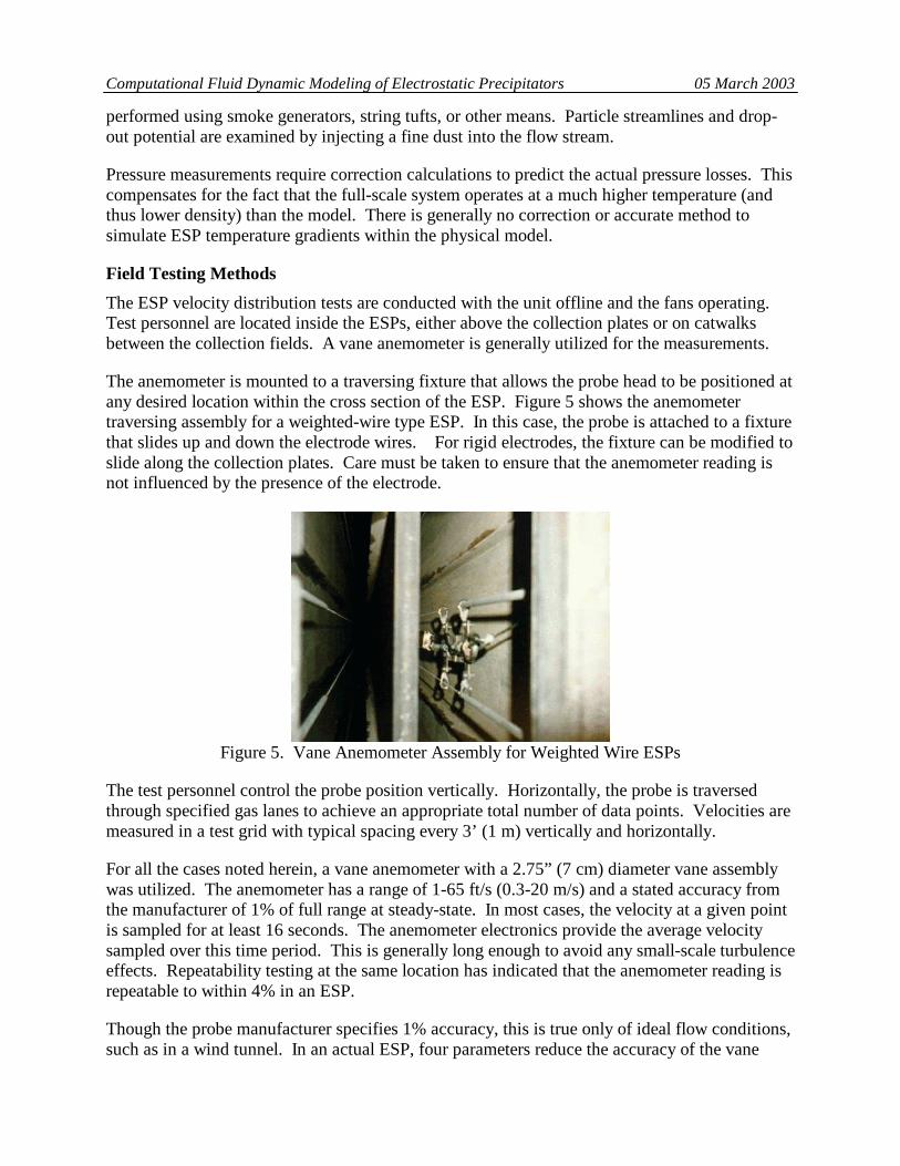
The anemometer is mounted to a traversing fixture that allows the probe head to be positioned at any desired location within the cross section of the ESP. Figure 5 shows the anemometer traversing assembly for a weighted-wire type ESP. In this case, the probe is attached to a fixture that slides up and down the electrode wires. For rigid electrodes, the fixture can be modified to slide along the collection plates. Care must be taken to ensure that the anemometer reading is not influenced by the presence of the electrode.

Figure 5. Vane Anemometer Assembly for Weighted Wire ESPs

The test personnel control the probe position vertically. Horizontally, the probe is traversed through specified gas lanes to achieve an appropriate total number of data points. Velocities are measured in a test grid with typical spacing every 3’ (1 m) vertically and horizontally.

For all the cases noted herein, a vane anemometer with a 2.75” (7 cm) diameter vane assembly was utilized. The anemometer has a range of 1-65 ft/s (0.3-20 m/s) and a stated accuracy from the manufacturer of 1% of full range at steady-state. In most cases, the velocity at a given point is sampled for at least 16 seconds. The anemometer electronics provide the average velocity sampled over this time period. This is generally long enough to avoid any small-scale turbulence effects. Repeatability testing at the same location has indicated that the anemometer reading is repeatable to within 4% in an ESP.

Though the probe manufacturer specifies 1% accuracy, this is true only of ideal flow conditions, such as in a wind tunnel. In an actual ESP, four parameters reduce the accuracy of the vane


anemometer measurement: flow unsteadiness, velocity stratification, flow angularity, and particulate deposition. The velocity fluctuations are generally minimized by time-averaging over an extended sampling period, but low-frequency unsteadiness can still disturb the measurements. As mentioned above, using a 16-second average usually provides 4% repeatability, but in some instances longer sampling times have been necessary.

Velocity stratification causes a problem because the probe design is such that it requires a constant velocity over its measurement region. This region is the diameter of the vane assembly. If the probe is located in a region where a velocity gradient exists, it does not accurately provide an indication of the average velocity within that region. Velocity stratification can be an issue when measuring ESPs with rigid electrodes, large structural ribs or elements on the collection plates, or other obstacles upstream of the measurement location. In addition, measuring too close to a perforated plate or other flow control device can result in velocity stratification.

Flow angularity is another issue that influences the accuracy of the vane anemometer reading. The vane anemometer does not provide an accurate means of measuring a particular component of velocity. Thus, when the flow travels at any angle other than parallel to the vane rotational axis, a measurement error can result. Test personnel must take this into consideration when selecting measurement locations, particularly near the inlet of the ESP where angularity is generally highest.

In some cases due to outage schedules, testing must occur with the ESP in a dirty condition. This may include particulate deposits on collection plates, electrodes, and flow control devices. Sometimes these deposits can influence the local flow characteristics. Airborne particulate can degrade the performance of the vane anemometer.

Despite these detractions, a vane anemometer is still the probe of choice for ESP velocity distribution tests. Hot wire or hot mandrel probes, another option, can suffer from the same issues mentioned above but with greater sensitivity. They are generally much more susceptible to damage and fouling in the dirty environment of the ESP. Katz has mentioned concerns over use of the hot wire as well [5].

Data Comparisons

A direct comparison of field test data to CFD model results is made for ten ESPs. Three specific case studies are discussed in detail to relate the general comparison process; then all cases are summarized.

There are several statistical methods available to compare the data. Four specific quantitative comparisons are made:

1. Contour plots. The test and model data at the available locations are plotted as color contour plots indicating velocity magnitude in the axial (primary) flow direction. The model and test data are normalized by dividing by the appropriate average velocity. This allows the velocity distributions to be compared on an equivalent color scale.


2. Comparison of flow distribution statistics. The velocity deviation from a target flow distribution is a typical statistic desired by ESP designers and owners. This is generally quantified at both the ESP inlet and outlet plane in one of two ways:

a. Standards set by the Institute of Clean Air Companies (ICAC). The ICAC guidelines of Publication EP-7 [6] require that “Within the treatment zone near the inlet and outlet faces of the precipitator collection chamber, the velocity pattern shall have a minimum of 85% of the velocities not more than 1.15 times the average velocity and 99% of the not more than 1.40 times the average velocity.”

b. Percent RMS deviation of the measured/modeled velocity versus the average velocity. The percent RMS is calculated by the following formula:

%RMS = ( )( ) 1

1002

−−

∑∑

i

vv

vavgi

avg

where vi = velocity at select grid point vavg = average velocity over entire plane i = grid point counter

Thus, the percent RMS quantifies what percent of the flow area is outside of one standard deviation of all velocities that exist at that plane. The typical goal in industry is to achieve a Percent RMS of less than 15% at the ESP inlet and outlet planes. Some ESP personnel target an even tighter tolerance of 10% at the ESP outlet plane. Percent RMS is a useful statistic for two reasons. First, it includes low velocities (e.g., below 0.85 times the average velocity) whereas the ICAC standards focus on only the high velocities. Second, it allows comparisons to velocity distribution targets other than perfectly uniform flow. The local target velocity is simply inserted into the summation above in place of the average velocity.

3. Point-by-point data deviations. This is the most rigorous evaluation, as every single data point is compared spatially. The results of this comparison are plotted in a histogram form, indicating the quantity of points that match between test data and model for a given accuracy tolerance. The deviation as plotted is calculated as follows:

Deviation = testavg

ielitest

v

fvv

−

−− ∗− mod

where vmodel-i = model predicted velocity at select grid point vtest-i = measured velocity at select grid point f = vavg-test / vavg-model

vavg-test = average velocity over entire plane from test data i = grid point counter

4. Overall Correlation Factor. This is basically a single number that allows comparison of all ESP cases regardless of geometry. The Correlation Factor is defined as follows:


Correlation Factor = ( )

( ) 1

1002

mod

−∗−

∑∑ −−

− i

fvv

vielitest

testavg

where vmodel-i = model predicted velocity at select grid point vtest-i = measured velocity at select grid point f = vavg-test / vavg-model

vavg-test = average velocity over entire plane from test data i = grid point counter

Thus, the Correlation Factor is the Percent RMS between the test data and the model results on a point-by-point basis. A Correlation Factor of 15% implies that in a rigorous spatial comparison of all data points at a given plane, 66% (one standard deviation) of the model velocities match the data to within 15%.

One detail should be noted regarding the plots and calculations described above. The CFD results and measurements in the physical models generally have a much finer test grid than the field test data. A typical CFD model has over 3000 grid points where velocity values are available for each measurement plane. The physical scale models have on the order of 450 grid points while the test data generally has less than 100 grid points. Since the models provide finer detail than the field data, the model results are interpolated from their original grid onto the coarser grid of the field test data. This allows the plots and data comparisons to be most representative. The differences in the grid density are shown graphically in Figure 6.

Figure 6. Comparison of Velocity Data Grid Points.

Case Study 1 – Southeastern U.S. Coal-fired Power Station

A particular 440 MW coal-fired unit in the Southeastern U.S. (utility name withheld) includes a large, single chamber electrostatic precipitator. Field testing and CFD modeling efforts were performed to assess ESP flow characteristics. A physical scale model was utilized to design the original ESP flow control devices in the early 1970s. Thus, data exists to compare both model types to the test data for the baseline ESP configuration. The CFD model was then utilized to develop modifications to the flow control devices. The test data were recorded at two planes in the flow direction: 1) At the beginning of the first collection field (“Inlet Plane”) and 2) At the end of the last collection field (“Outlet Plane”).

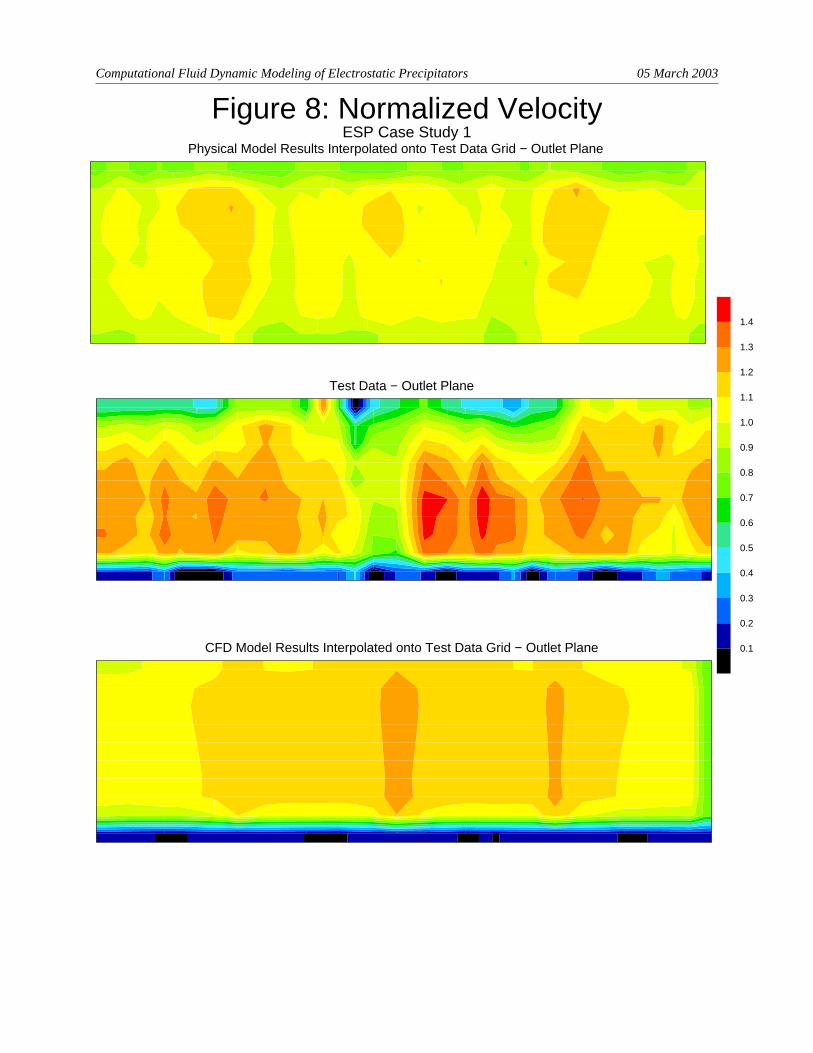
Color contour plots for each of these cases are shown in Figures 7 and 8. These plots indicate the velocity magnitude in the primary (axial) flow direction at the two test planes, respectively. In each figure, the measured test data are plotted in the center; the physical model results are at the top and the CFD model results are at the bottom. Examining the test data for both planes, it is apparent that the model results are much smoother than the test data. This is due to the

Test Data − Inlet Plane

Physical Model Results Interpolated onto Test Data Grid − Inlet Plane

CFD Model Results Interpolated onto Test Data Grid − Inlet Plane 0.1

0.2

0.3

Figure 7: Normalized Velocity

0.4

0.5

0.6

0.7

0.8

0.9

1.0

1.1

1.2

1.3

1.4

ESP Case Study 1


CFD Model Results Interpolated onto Test Data Grid − Outlet Plane

Test Data − Outlet Plane

Physical Model Results Interpolated onto Test Data Grid − Outlet Plane

0.1

0.2

0.3


0.4

0.5

0.6

0.7

0.8

0.9

1.0

1.1

1.2

1.3

1.4

ESP Case Study 1



coarseness of the test grid and the fact that the field measurements have a higher sensitivity to local structural features.

There are some noticeable trends in the velocity patterns of the measured test data. Very high velocities (greater than 1.4 times the average) exist along the lower half of the Inlet Plane. At the very bottom, a row of near-zero velocities is measured, and a low velocity region exists along the right wall. The physical model results do not match these trends at all, while the CFD model only captures some of the trends. This includes the region of high velocity in the lower half of the plane, but the CFD model does not match the magnitude of these high velocity regions. It does predict, however, a zero velocity region in the bottom row of measurement points.

At the Outlet Plane, the test data seem to indicate a higher velocity region in the middle of the plane all the way across the ESP. A repeating pattern exists of the highest velocities. Similar to the Inlet Plane, a row of near-zero velocities exists at the bottom. The models also indicate higher velocities in the middle of the ESP, including some appearance of the repeating high-velocity columns, but not to the same magnitude as the test data. The CFD model also predicts the low velocity region at the bottom.

In examining these plots, one might conclude that correlation is not strong for either model, but the CFD model provides a closer match than the physical model.

Tables 1 through 3 provide a comparison of flow distribution statistics for the ESP for the Inlet Plane and Outlet Plane for this ESP.

% RMS from goal Configuration Test Data CFD Model Physical Model

Inlet Plane 34.5 37.0 14.2 Outlet Plane 35.1 30.8 11.9

Table 1. Case Study 1 Flow Distribution Statistics - %RMS

ICAC Standards: % Less Than 115% of Average Configuration Test Data CFD Model Physical Model


Table 2. Case Study 1 Flow Distribution Statistics – ICAC 115%

ICAC Standards: % Less than 140% of Average Configuration Test Data CFD Model Physical Model

Inlet Plane 91.9 100 100 Outlet Plane 97.5 100 100

Table 3. Case Study 1 Flow Distribution Statistics – ICAC 140%

It is evident for both planes that the CFD model provides a much better prediction of the %RMS and the ICAC 115% conditions than the physical scale model. The physical model appears to over-predict the flow uniformity indicated by these flow distribution statistics in all cases, while the CFD model over-predicts ICAC conditions, most notably for the 140% requirement. As shown, the physical model predicted ICAC compliance. Due to the large differences between


the physical model and the test data, a closer inspection of the physical model was deemed necessary. Although the physical modeling report indicates that it was run in the turbulent regime, the poor agreement with test data flow statistics leaves questions about whether the Reynolds Number was calculated based on the correct hydraulic diameter.

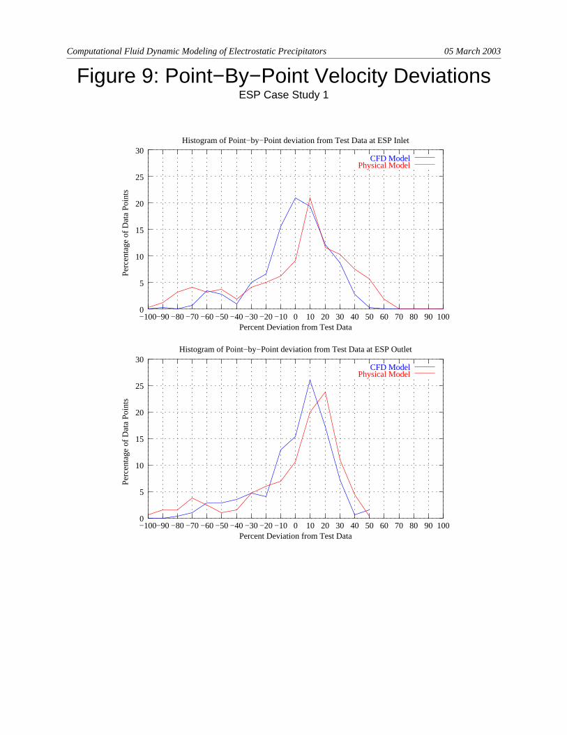
Point-by-point deviations between the model results and the test data are plotted in the histograms of Figure 9. These plots present the number of data points which are within a given percentage deviation from the test data. For instance, the first histogram shows a peak near (0,21) for the CFD model. This indicates that about 21% of the data points from the CFD model had a deviation from the test data of between –5% and 5%. Similarly, the physical model curve shows a peak near (10,21), which indicates that about 21% of the data points had a deviation from the test data of between 5% and 15%. Visually, these plots show similar correlation for both models, although there are some points noted for both the CFD model and physical scale model that are greater than 50% off from the test data. Most of these points are found on the bottom row of data (which shows very low velocities in the test data), and along the right side of the Inlet Plane (where test data is also quite low). It is possible that the region of low flow velocities is a result of test data inaccuracy. That being said, the histogram curves for the CFD model seem to be more centrally located around 0% deviation.

For the CFD model, approximately 75% of the model predictions fall within a +/-25% error band from the test data at the Inlet Plane. For the physical model, 52.8% of values are within +/-25% at the same plane. At the Outlet Plane, 75% of the CFD model predictions fall within a +/-25% error band, as compared to 66% for the physical model.

The Correlation Factor for this ESP is shown in Table 4. As indicated, the CFD model features an average Correlation Factor of 24.3% and the physical model provides a Correlation Factor of 34.2%. This implies much better correlation for the CFD model.

Correlation Factor Configuration CFD Model Physical Model

Inlet Plane 24.3 37.2 Outlet Plane 24.3 31.2

Table 4. Case Study 1 ESP Correlation Factor

The color contour plots seem to indicate better correlation of the CFD model to the test data at the Inlet Plane, but similar correlation of both models at the Outlet Plane. The flow distribution statistics, the point-by-point data comparisons, and Correlation Factor indicate better correlation of the CFD model at both planes. Although it is believed that future efforts will drive correlation factors lower, this level of correlation has proved to be enough to promote the CFD model as a useful engineering tool. In the case of this ESP, the correlation of the CFD model was deemed quite adequate to develop design recommendations. Results of flow conditions after the design phase are not yet available.

Case Study 2 – Western U.S. Coal-fired Power Station

ESP field testing and physical modeling were performed for a 326 MW coal fired power station in 1999. The unit has two precipitators with two chambers each. A CFD modeling study was completed in 2000. The test data were compared to results of each model study for the baseline

Figure 9: Point−By−Point Velocity DeviationsESP Case Study 1

0

5

10

15

20

25

30

−100−90 −80 −70 −60 −50 −40 −30 −20 −10 0 10 20 30 40 50 60 70 80 90 100

Perc

enta

ge o

f D

ata

Poin

ts

Percent Deviation from Test Data

Histogram of Point−by−Point deviation from Test Data at ESP Outlet

CFD ModelPhysical Model

0

5

10

15

20

25

30

−100−90 −80 −70 −60 −50 −40 −30 −20 −10 0 10 20 30 40 50 60 70 80 90 100

Perc

enta

ge o

f D

ata

Poin

ts


Histogram of Point−by−Point deviation from Test Data at ESP Inlet




configuration. The CFD model was then utilized to develop modifications to the flow control devices. The test data were recorded at two planes in the flow direction: 1) At the beginning of the first collection field (“Inlet Plane”) and 2) At the end of the last collection field (“Outlet Plane”).

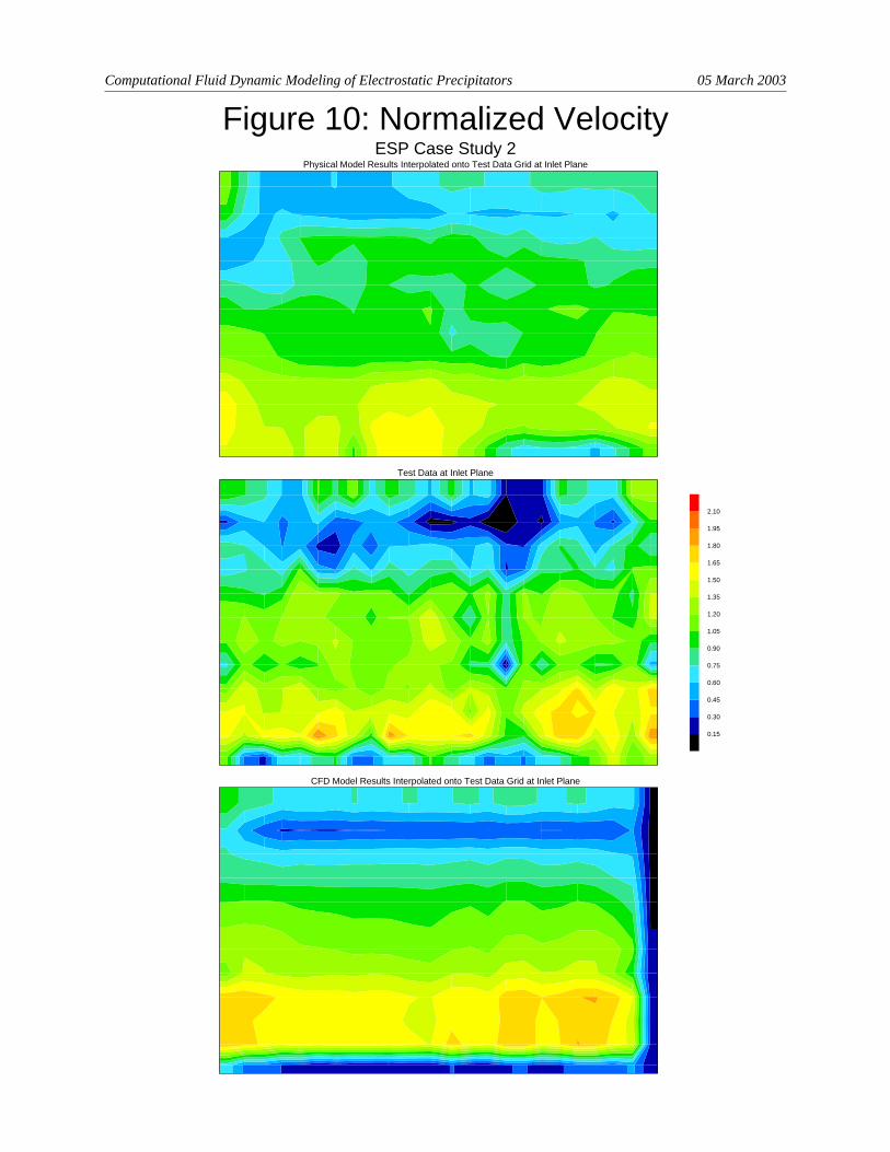
Color contour plots for each of these cases are shown in Figures 10 and 11. It is evident in these plots that the intent is not to meet standard ICAC uniformity standards. Instead, a specified velocity profile was targeted based on Skewed Gas Flow TechnologyTM principles of Stothert Engineering, Ltd [7].

These plots present the velocity magnitude in the primary (axial) flow direction at the two test planes. They indicate that both the CFD and physical models capture the trends at both the Inlet Plane and the Outlet Plane. As can easily be seen, regions of higher flow velocity exist at the bottom of the Inlet Plane and the top of the Outlet Plane. At both planes, the physical model shows a lesser degree of velocity “skew” than do either the CFD model or the test data.

Tables 5 through 7 provide a comparison of flow distribution statistics for this ESP for the Inlet and Outlet Planes. Note that the %RMS and comparisons to ICAC standards have been modified, since the target velocity is non-uniform. Instead, %RMS and the percent of area with flow velocities less than 115% and 140% of the local target velocity is calculated.



Table 5. Case Study 2 ESP Flow Distribution Statistics - %RMS

% Less than 115% of Goal Velocity Configuration Test Data CFD Model Physical Model


Table 6. Case Study 2 ESP Flow Distribution Statistics – 115%

% Less than 140% of Goal Velocity Configuration Test Data CFD Model Physical Model


Table 7. Case Study 2 ESP Flow Distribution Statistics – 140%

At the Inlet Plane, the CFD model under-predicts the flow uniformity indicated by the %RMS and 115% conditions, while the physical model significantly over-predicts the uniformity as seen by the same figures. As can be seen on Figure 10, the physical model does not capture the highest velocities measured near the bottom of the inlet. While the CFD model predicts a fairly accurate peak velocity, it predicts a larger area of high velocities than measured. For this reason, the CFD model slightly under-predicts the 140% condition, while the physical model over-predicts the same value.

Physical Model Results Interpolated onto Test Data Grid at Inlet Plane

Test Data at Inlet Plane

CFD Model Results Interpolated onto Test Data Grid at Inlet Plane

0.15

0.30

0.45

Figure 10: Normalized VelocityESP Case Study 2

0.60

0.75

0.90

1.05

1.20

1.35

1.50

1.65

1.80

1.95

2.10


Physical Model Results Interpolated onto Test Data Grid at Outlet Plane

Test Data at Outlet Plane

CFD Model Results Interpolated onto Test Data Grid at Outlet Plane

0.17

0.33

0.50

Figure 11: Normalized VelocityESP Case Study 2

0.67

0.83

1.00

1.17

1.33

1.50

1.67

1.83

2.00

2.17

2.33



At the Outlet Plane, the CFD model slightly under-predicts the %RMS, while the physical model falls far short. This is due to the fact that the physical model does not capture the high velocities near the top of the Outlet Plane (Figure 11). Both models do a good job at predicting the ICAC 115% condition, although the physical model does so in a non-intuitive manner. The region of the flow field which is highest above the target velocity in the physical model is in the lower half of the Outlet Plane. This is a result of the fact that the physical model predicts a skew level smaller than either the target or the measured skew level at the Outlet Plane.

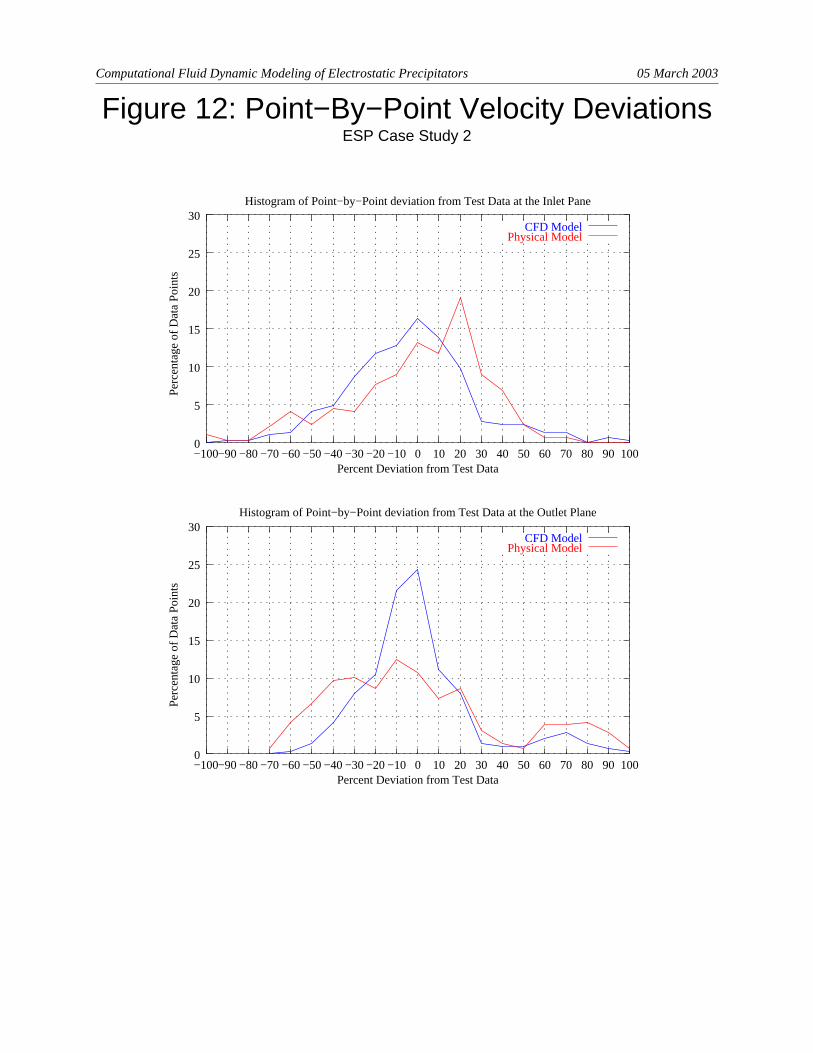
For the ESP baseline configuration, point-by-point deviations between the model results and the test data are plotted in the histograms of Figure 12. These plots show that 65% of the CFD model predictions fall within a +/-25% error band from the test data at the inlet, compared to 61% for the physical model. The same analysis at the Outlet Plane shows 75% of the CFD model predictions fall within the +/-25% error band, compared to 48% for the physical model.

The Correlation Factor for the baseline case is shown in Table 8. As indicated, the CFD model features an average Correlation Factor of 32.1% and the physical model provides a Correlation Factor of 36.6%. The physical model correlates somewhat better at the Inlet Plane and the CFD model better at the Outlet Plane.


Inlet Plane 37.0 32.4 Outlet Plane 27.2 40.8


The flow distribution statistics, the color contour plots, point-by-point data comparisons and the Correlation Factor generally indicate a similar correlation at the Inlet Plane (with the physical model correlating slightly better), but a better correlation of the CFD model at the Outlet Plane. All four data comparisons have to be taken into consideration and evaluated based on the goals of the modeling project. In this particular case, since SGFTTM was involved, the local velocity patterns at the ESP Outlet Plane were quite important. The CFD model was thus utilized to optimize the design of the outlet perforated plate in order to achieve the desired effects. After installation of the modifications developed through use of the CFD model, a reduction in particulate emissions was noted over the baseline case which was designed with the physical model.

Case Study 3 – Canadian Coal-fired Power Station

The ESP analyzed in this case is for a 385 MW unit with two precipitators having four chambers each. The flow control devices were designed using a physical model in 1979. In 1998, field testing was performed to assess ESP flow characteristics. A CFD model baseline study was performed in 1999 and the test data were compared to physical scale model and CFD model results. The CFD model was then utilized to develop modifications to the flow control devices. The test data were recorded at three planes in the flow direction: 1) At the beginning of the first collection field (“Inlet Plane”), 2) Between the first and second collection fields (“A/B Plane”), and 3) At the end of the last collection field (“Outlet Plane”).


0

5

10

15

20

25

30

−100−90 −80 −70 −60 −50 −40 −30 −20 −10 0 10 20 30 40 50 60 70 80 90 100

Perc

enta

ge o

f D

ata

Poin

ts


Histogram of Point−by−Point deviation from Test Data at the Outlet Plane


0

5

10

15

20

25

30

−100−90 −80 −70 −60 −50 −40 −30 −20 −10 0 10 20 30 40 50 60 70 80 90 100

Perc

enta

ge o

f D

ata

Poin

ts


Histogram of Point−by−Point deviation from Test Data at the Inlet Pane




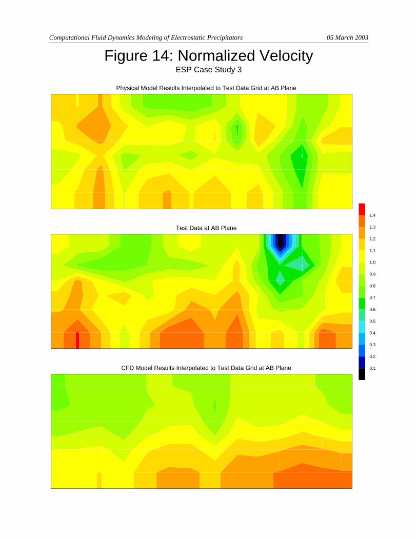
Color contour plots for each of these cases are shown in Figures 13 through 15. These plots present the velocity magnitude in the primary (axial) flow direction at the three test planes. These plots indicate that both the CFD and physical models capture the trends at the A-B Plane and the Outlet Plane. Neither compares very well to the test data from the Inlet Plane. This has been traced to the fact that severe flow angularity exists in the upper and lower portions of the Inlet Plane. Thus, the velocity measurements at this plane do not actually represent the magnitude in the axial direction.

Tables 9 through 11 provide a comparison of flow distribution statistics for the ESP for the Inlet Plane, A-B Plane and Outlet Plane.


Inlet Plane 44.2 33.9 40.3 A-B Plane 22.5 14.7 24.7

Outlet Plane 38.0 18.7 25.0

Table 9. Case Study 3 ESP Flow Distribution Statistics - %RMS



Outlet Plane 55.1 73.5 81.6

Table 10. Case Study 3 ESP Flow Distribution Statistics – ICAC 115%



Outlet Plane 98.0 100.0 100.0

Table 11. Case Study 3 ESP Flow Distribution Statistics – ICAC 140%

The high %RMS for the Inlet Plane is another indication that flow angularity is affecting the interpretation of the test data. It is evident for the A-B Plane and Outlet Plane, however, that the CFD model under-predicts the %RMS considerably. The physical model under-predicts for only the Outlet Plane and to a slightly lesser degree than the CFD model. The CFD model, however, shows better agreement with the test data in ICAC conditions than does the physical model.

For the baseline configuration, point-by-point deviations between the model results and the test data are plotted in the histograms of Figure 16. These plots show how poor the correlation is for the Inlet Plane where flow angularity is prevalent. The correlation for the A-B and Outlet Planes appear very similar for both the CFD and physical scale models. These histograms indicate that 43.8% of the CFD model predictions fall within a +/-25% error band from the test data at the Inlet Plane, compared to 37.5% for the physical model. At the A-B Plane, the same analysis yields 82.1% of the CFD model predictions falling within a +/-25% error band, compared with 70.2% for the physical model. Lastly, at the Outlet Plane, the same analysis yields 83.7% of the

Test Data at Inlet Plane

CFD Model Results Interpolated to Test Data Grid at Inlet Plane

Physical Model Results Interpolated to Test Data Grid at Inlet Plane

0.12

0.24

0.36


0.48

ESP Case Study 3

0.60

0.72

0.84

0.96

1.08

1.20

1.32

1.44

1.56

1.68

Computational Fluid Dynamics Modeling of Electrostatic Precipitators 05 March 2003

Physical Model Results Interpolated to Test Data Grid at AB Plane

Test Data at AB Plane

CFD Model Results Interpolated to Test Data Grid at AB Plane 0.1

0.2

0.3


0.4

ESP Case Study 3

0.5

0.6

0.7

0.8

0.9

1.0

1.1

1.2

1.3

1.4

Computational Fluid Dynamics Modeling of Electrostatic Precipitators 05 March 2003

CFD Model Results Interpolated to Test Data Grid at Outlet Plane

Test Data at Outlet Plane

Physical Model Results Interpolated to Test Data Grid at Outlet Plane

0.1

0.2

0.3


0.4

ESP Case Study 3

0.5

0.6

0.7

0.8

0.9

1.0

1.1

1.2

1.3

1.4



0

5

10

15

20

25

30

−100−90 −80 −70 −60 −50 −40 −30 −20 −10 0 10 20 30 40 50 60 70 80 90 100

Perc

enta

ge o

f D

ata

Poin

ts


Histogram of Point−by−Point deviation from Test Data at the Inlet Plane


0

5

10

15

20

25

30

−100−90 −80 −70 −60 −50 −40 −30 −20 −10 0 10 20 30 40 50 60 70 80 90 100

Perc

enta

ge o

f D

ata

Poin

ts


Histogram of Point−by−Point deviation from Test Data at the AB Plane


0

5

10

15

20

25

30

−100−90 −80 −70 −60 −50 −40 −30 −20 −10 0 10 20 30 40 50 60 70 80 90 100

Perc

enta

ge o

f D

ata

Poin

ts


Histogram of Point−by−Point deviation from Test Data at the Outlet Plane




CFD model predictions falling within a +/-25% error band, compared with 72.4% for the physical model.

There are some points noted for both the CFD model and physical scale model that are greater than 50% off from the test data. The specific points where this occurs are near the bottom of the ESP. As can be observed in the color contour plots, several zero velocity readings were obtained (black test data points). This indicates that the presence of some structural element is affecting the test probe. It appears that this structure is not included geometrically in either model.

The Correlation Factor for the baseline case is shown in Table 12. The Inlet Plane is not included due to the flow angularity issues. As indicated, the CFD model features an average Correlation Factor of 24.5% and the physical model provides a Correlation Factor of 28.4%. The physical model average is higher at the Outlet Plane, where there are some points greater than 80% off of the test data as noted in the histograms. In general, both models provide similar accuracy when all data points are compared directly, with the CFD model correlating slightly better.


A-B Plane 21.2 24.8 Outlet Plane 27.8 31.9


The flow distribution statistics and the color contour plots seem to indicate better correlation of the physical scale model to the test data, but the point-by-point data comparisons and Correlation Factor indicate better correlation of the CFD model.

In the case of this ESP, the correlation of the CFD model was deemed quite adequate to develop design recommendations. The design objective was to incorporate SGFTTM per Stothert Engineering specifications. After installation of the modifications developed through use of the CFD model, a significant reduction in particulate emissions over the baseline case was recorded.

Summary – All Case Studies

All case studies are for coal-fired power stations in North America. An indication of plant size and location is provided in Table 13. Contour plots and histograms from all 10 case studies are not included for brevity. Flow statistics and Correlation Factors for each case are presented numerically in Tables 14 through 16 and graphically in Figures 17 through 20.

Case Study Plant Size Location Case Study Plant Size Location 1 440 MW Southeast U.S. 6 893 MW Midwest U.S. 2 326 MW Western U.S. 7 893 MW Midwest U.S. 3 385 MW Canada 8 952 MW Southeast U.S. 4 441 MW Southeast U.S. 9 952 MW Southeast U.S. 5 446 MW Southeast U.S. 10 385 MW Canada

Table 13. All Case Studies - Plant Descriptions


% RMS from goal

Case Study

Data Plane

Location

Test Data

CFD

Model

Physical Model

1 Inlet 34.5 37.0 14.2 Outlet 35.1 30.8 11.9 2 Inlet 33.4 42.0 20.1 Outlet 34.7 27.8 17.8 3 Inlet 44.2 33.9 40.3 AB 22.5 14.7 24.7 Outlet 38.0 18.7 25.0 4 AB 28.5 32.1 15.2 5 Outlet 32.9 24.3 29.7 6 Inlet 11.2 4.3 n/a Outlet 8.9 4.5 n/a 7 Inlet 8.6 3.4 n/a Outlet 8.3 4.6 n/a 8 Inlet 39.6 22.3 n/a Outlet 11.2 10.3 n/a 9 Inlet 28.7 22.8 n/a Outlet 12.7 11.2 n/a

10 AB 48.1 37.9 n/a Outlet 32.2 20.1 n/a

Table 14. All Case Studies Figure 17. All Case Studies Flow Distribution Statistics - %RMS Flow Distribution Statistics - %RMS

ICAC Standards: % Less

than 115% of Goal ICAC Standards: % Less

than 140% of Goal Case Study

Data Plane Location

Test Data

CFD Model

Physical Model

Test Data

CFD Model

Physical Model

1 Inlet 63.5 61.5 86.5 91.9 100 100 Outlet 78.8 76.7 72.6 97.5 100 100 2 Inlet 63.5 61.5 86.5 93.7 91.0 99.7 Outlet 78.8 76.7 72.6 86.8 90.6 92.0 3 Inlet 60.7 61.6 69.6 78.6 86.6 96.4 AB 75.0 80.9 84.5 98.8 100.0 100.0 Outlet 55.1 73.5 81.6 98.0 100.0 100.0 4 AB 68.5 74.3 95.2 93.1 86.5 100 5 Outlet 66.9 67.5 90.6 96.9 100 100 6 Inlet 96.5 100 n/a 100 100 n/a Outlet 100 97.9 n/a 100 100 n/a 7 Inlet 94.4 100 n/a 100 100 n/a Outlet 98.6 97.9 n/a 100 100 n/a 8 Inlet 66.9 75.0 n/a 84.4 97.2 n/a Outlet 90.0 94.4 n/a 100 100 n/a 9 Inlet 71.9 82.8 n/a 92.5 97.8 n/a Outlet 88.9 91.9 n/a 100 100 n/a

10 AB 58.7 61.9 n/a 79.4 89.7 n/a Outlet 88.1 100 n/a 94.0 100 n/a

Table 15. All Case Studies - Flow Distribution Statistics – ICAC Conditions

%RMS Correlation

0

10

20

30

40

50

60

1I 1O 2I 2O 3I 3AB 3O 4AB 5O 6I 6O 7I 7O 8I 8O 9I 9O 10AB 10O

Case

% R

MS

Test Data CFD Model Physical Model


Figure 18. All Case Studies Figure 19. All Case Studies Flow Distribution Statistics – ICAC 115% Flow Distribution Statistics – ICAC 140%

Correlation Factor

Case Stud

y

Data Plane

Location

CFD

Model

Physic

al Model

1 Inlet 24.3 37.2 Outlet 24.3 31.2

2 Inlet 37.0 32.4 Outlet 27.2 40.8

3 AB 21.2 24.8 Outlet 27.8 31.9

4 AB 35.0 31.2 5 Outlet 25.9 31.3 6 Inlet 10.3 n/a Outlet 10.6 n/a

7 Inlet 8.4 n/a Outlet 10.8 n/a



10 AB 33.4 n/a Outlet 21.8 n/a

Table 16. All Case Studies Figure 20. All Case Studies - Correlation Factor Correlation Factor

Analyzing the flow statistics, it appears that both model types have similar accuracy when compared to the test data. On average using all 10 case studies, the Correlation Factor for the

Correlation Factor Summary

0

5

10

15

20

25

30

35

40

45

1I 1O 2I 2O 3I 3AB 3O 4AB 5O 6I 6O 7I 7O 8I 8O 9I 9O 10AB

Case

Co

rrel

atio

n F

acto

r

CFD Model Physical Model

ICAC 115% Condition Correlation

0

20

40

60

80

100

120

1I 1O 2I 2O 3I3A

B 3O 4AB 5O 6I 6O 7I 7O 8I 8O 9I 9O

10AB

10O

Case

% L

ess

than

115

% o

f G

oal


ICAC 140% Condition Correlation

0

20

40

60

80

100

120

1I 1O 2I 2O 3I3A

B 3O 4AB 5O 6I 6O 7I 7O 8I 8O 9I 9O

10AB

10O

Case

% L

ess

than

140

% o

f G

oal



CFD models is 23.5 (27.8 using only studies where the physical model also existed) and for the physical models 32.6, as indicated in Table 17.

Correlation Factor Configuration CFD Model Physical

Model Inlet Plane – All Models 27.2 34.7 AB Plane – All Models 29.9 28.0

Outlet Plane – All Models 18.6 33.8

Inlet Plane where both Models Exist 30.6 34.7 AB Plane where both Models Exist 28.1 28.0

Outlet Plane where both Models Exist 26.3 33.8

All Planes 23.5 32.6 All Planes where both Models Exist 27.8 32.6

Table 17. Average Correlation Factor For All Case Studies

Summary / Conclusions

The comparisons of CFD and physical model results presented herein indicate that both modeling types provide similar accuracy with respect to gas flow velocity patterns within an ESP. On average using all 10 case studies, the Correlation Factor for the CFD models is 23.5 (27.8 using only studies where the physical model also existed) and for the physical models 32.6. This has been shown to be a high enough degree of correlation to allow modeling to be a useful engineering tool.

It is believed that increased correlation to test data may be accomplished through careful attention to modeling methods, as well as through careful attention to methods of comparison. Specifically in the case of CFD modeling, smaller structural elements must be built into the model as computer power allows. Details of the mounting structure associated with flow control devices should be considered. Whenever possible, detailed inspections should document as-installed geometry of flow control devices. These measurements should be used to confirm the ESP drawings that are used to build the model. When comparing test data to model data, care should be taken to precisely identify each test data point location within the model. Model data should be interpolated to the same grid as the test data in order to make an appropriate comparison.

Acknowledgements

The authors wish to thank all contributing ESP owners and manufacturers for providing facilities, data, and/or information this paper.

References

Nelson, R., VISCOUS Users Guide, Airflow Sciences Corporation, 1993.

Patankar, S., Numerical Heat Transfer and Fluid Flow, Hemisphere Publishing, 1980.


Lindeburg, M., Mechanical Engineering Reference Manual, Professional Publications, Inc., Belmont, CA, 1995, p. 3-33.

Gretta, W.J., and Grieco, G.J., “Consideration of Scale in Physical Flow Modeling of Air Pollution Control Equipment,” International Joint Power Generation Conference, 1995.

Katz, J., The Art of Electrostatic Precipitation, Precipitator Technology Inc., 1979.

Institute of Clean Air Companies, “Electrostatic Precipitator Gas Flow Model Studies,” Publication EP-7, January 1997.

Hein, A., “A New Concept in Electrostatic Precipitator Gas Distribution,” American Power Conference, 1988.

Date post:	08-Feb-2018
Category:	Documents
Upload:	vonguyet
View:	221 times
Download:	0 times

COMPUTATIONAL FLUID DYNAMIC MODELING OF · PDF fileCOMPUTATIONAL FLUID DYNAMIC MODELING OF...

Documents