Page 1
COMPUTATIONAL FLUID DYNAMICS AND POPULATION BALANCE MODELING
OF PARTICULATE SYSTEMS
BY
MICHAEL LAWRENCE RASCHE
THESIS
Submitted in partial fulfillment of the requirements
for the degree of Master of Science in Chemical Engineering
in the Graduate College of the
University of Illinois at Urbana-Champaign, 2010
Urbana, Illinois
Adviser:
Professor Richard D. Braatz
Page 2
ii
Abstract
Computational models are developed in an effort to aid in the design of process equipment for
the crystallization of pharmaceutical compounds. The models focus on the combination of
population balance equations and computational fluid dynamics software. For the simulation of
antisolvent crystallization, knowledge of kinetics at high supersaturation are necessary. Chapter
2 describes the concentration profile within a high-throughput evaporation platform that can be
used to create conditions of high supersaturation for the study of crystal polymorphs as well as
nucleation and growth kinetics. An equation is derived for the maximum concentration
difference within an evaporating droplet. Chapter 3 models the secondary nucleation phenomena
of breakage due to ultrasonic irradiation of crystals dispersed in a fluid. The simulation model is
used to estimate optimal kinetic parameters for the breakage kernel by comparison to
experimental data. Chapter 4 implements fouling along the walls in the simulation of cooling
crystallization of seeds in an agitated tank. Future goals include adding breakage and
aggregation/agglomeration to the model described in Chapter 4 and using the increasing
computational power of modern supercomputers to simulate the multiphase system.
Page 3
iii
Table of Contents
1 Introduction ........................................................................................................................................... 1 2 Transport Phenomena within a High-Throughput Evaporation Platform ............................................. 5
2.1 Introduction ................................................................................................................................... 5 2.2 Analysis ......................................................................................................................................... 7
3 Ultrasound-Induced Breakage ............................................................................................................. 12 3.1 Introduction ................................................................................................................................. 12 3.2 Methods ....................................................................................................................................... 13 3.3 Results ......................................................................................................................................... 19
4 Fouling in Cooling Crystallization ...................................................................................................... 24 4.1 Introduction ................................................................................................................................. 24 4.2 Methods ....................................................................................................................................... 27
5 Future Work ........................................................................................................................................ 32 6 Acknowledgments ............................................................................................................................... 34 7 References ........................................................................................................................................... 35
Page 4
1
1 Introduction
Nearly all pharmaceutical compounds are delivered in crystalline form, and those that are not
are nearly always purified by a series of crystallizations from solution. It is well-known that
crystal nucleation, growth, and aggregation can be sensitive to non-ideal mixing. This is
especially true for the antisolvent crystallizations that are used in the pharmaceutical industry to
crystallize thermally sensitive pharmaceuticals.i,ii
Most pharmaceutical compounds can
crystallize in multiple crystal forms known as polymorphs (each polymorph contains the same
molecules, but with the molecules stacked or oriented differently in the crystalline lattice). Each
polymorph can have different properties such as dissolution rate, solubility, and bioavailability,
and for that reason it is important for a pharmaceutical company to produce a single polymorph
reliably. The size and shape of the crystals are also important to be able to properly wash, filter,
and dry the crystals when they leave the crystallization process; that is, the control of the crystal
size and shape distribution (typically referred to as the “CSD”) is also important for the
production of crystals of high consistency. These crystallizations from solution usually occur in
agitated vessels.
Numerous experimental studies of antisolvent crystallization in an agitated vessel indicate
that the CSD and polymorphic form can depend strongly on the operating conditions, such as
agitation rate, mode of addition, addition rate, solvent composition, and size of the
crystallizer.iii,iv
Most variations in the operating conditions have a direct influence on the mixing,
which affects the localized supersaturation and thus the crystal product (the supersaturation is
the effective driving force for the nucleation and growth of crystals, related to the difference in
chemical potential between the solute concentration and its value at equilibrium conditions).
Because the dependence of nucleation and growth rates on supersaturation is highly system
Page 5
2
specific, determining the optimal process conditions that produce the desirable crystal product
can require numerous bench-scale laboratory experiments, which might not be optimal after the
scale-up of the crystallizer, as the mixing effects and spatial distribution of supersaturation can
be vastly different. A pressing issue for the pharmaceutical industry is the regulatory requirement
of consistency in the various chemical and physical properties of the crystals.v Such concerns
motivate the development of a computational model to simulate the antisolvent crystallization
process to quantify the effects of mixing on the product crystal characteristics such as the CSD,
which determines the bioavailability of the drug and efficiency of downstream processes (e.g.,
filtration and drying).
In recent years there have been significant advances in the simulation of the effects of non-
ideal mixing on crystal nucleation and growth.xxiii,vii
The most accurate of the currently available
methods couple three types of models:
1.) A macromixing model for simulating the fluid flow between cells in a computational
fluid dynamics (CFD) code (for industrial-scale agitated vessels, the Reynolds-averaged
Navier-Stokes equations are simulated),
2.) A micromixing model for the subgrid scale (for industrial-scale agitated vessels, this is
typically a multi-environment probability density function model), and
3.) A population balance model for the evolution of the crystal size distribution under
nucleation and growth.
Models 2 and 3 can be formulated in the form of reaction-diffusion-convection equations which
can be run simultaneously with the turbulent macromixing fluid dynamics equations by a general
CFD-solver. In the past this approach has been applied to simulate the effects of agitation speed
and antisolvent addition mode, rate, and position during scale-up on the crystal size distribution
Page 6
3
in an agitated semibatch vessel and the effects of varying inlet velocity in impinging jet
crystallization. The numerical algorithms and software have some limitations:
1.) Only crystallization kinetics that do not involve integrals were modeled, limiting the
kinetic processes to primary nucleation, growth, and dissolution, with no modeling of
secondary nucleation (that is, nucleation of crystals when crystals are already present in
the system), aggregation/agglomeration, and breakage/attrition. This limited the
simulations of the agitated tank to the early stages of antisolvent crystallization.
2.) The presence of solids was addressed by treating the suspension as a pseudo-
homogeneous phase with a spatial variation in the effective viscosity, limiting the
simulations to conditions in which the crystals are small enough to follow streamlines.
This thesis describes steps towards making such crystallization simulations more generally
useful in applications . Chapter 2 deals with determination of the mixedness within droplets in a
high-throughput crystallization platform that operates at high supersaturation to identify
polymorphs and determine crystallization kinetics. Such systems have the potential to determine
true crystallization nucleation and growth kinetic parameters needed in the aforementioned high-
fidelity impinging jet crystallizations. Chapter 3 explains an efficient numerical model of
breakage/attrition when crystals are exposed to ultrasonic waves. This work provides a
computationally efficient algorithm for including integrals in the population balance equations,
and extends past work model crystallization simulations in which ultrasonic waves are used to
influence the crystal size distribution. Chapter 4 describes a CFD-PBE model of crystal growth
and fouling during the cooling stage of crystallization in an agitated tank. The main extension of
this work is to model the effects of fouling, which can become an operational concern in the
continuous-flow crystallizers that are started to be investigated in the pharmaceutical industry.
Page 7
4
Finally, Chapter 5 discusses the next steps wherein the ideas in the previous three chapters will
be combined into a single model.
Page 8
5
2 Transport Phenomena within a High-Throughput Evaporation Platform
2.1 Introduction
The Food and Drug Administration (FDA) has pressured the crystallization industry to
adhere to “Quality by Design” through the use of process modeling tools in order to reduce
experimentation and obtain the desired product the first time.v In crystallization, this commonly
means creating product crystals with a narrow distribution with a desired mean size. One
effective method for creating crystals with a narrow size distribution is through the use of dual
impinging jet (DIJ) crystallizers. A high supersaturation environment is created by intersecting
high-velocity streams of saturated solution and antisolvent. The crystals produced in this manner
can then be efficiently grown to the desired size.vi
Downstream processes such as grinding and
milling, which cause reduction in crystal product size, are avoided completely, while separations
are made simpler due to particle size uniformity. DIJ crystallizers can be modeled provided that
the necessary high-supersaturation kinetics are available.vii
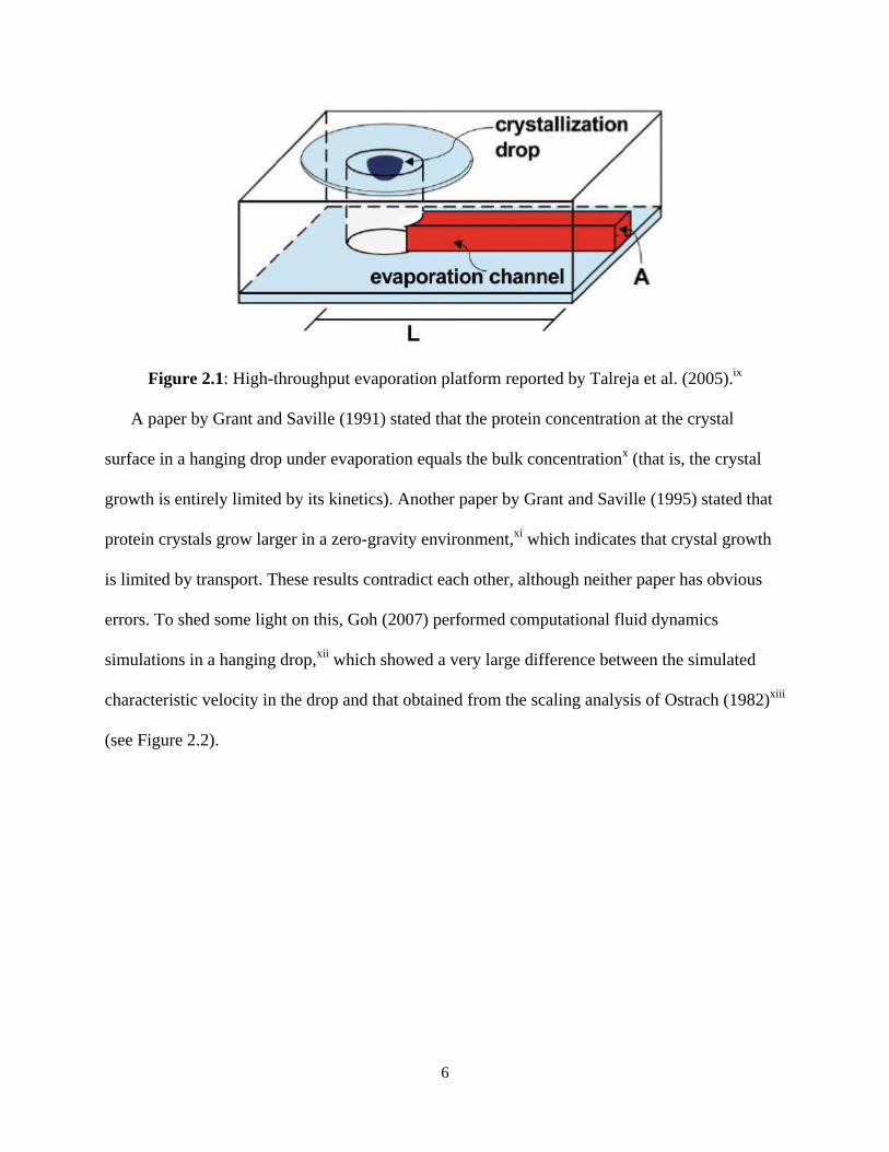
High-throughput evaporation platforms can be used to obtain high-supersaturation kinetics as
well as screen for polymorphs and effective solvents.viii
Many of these platforms, such as shown
in Figure 2.1 below, are based on the classic hanging drop experiment. The particular platform in
Figure 2.1 is made of a PDMS layer about 7 mm thick with a cylindrical evaporation chamber of
5 mm in diameter and an evaporation channel that is 5-10 mm long with a 250 250 to 1000
1000 micron cross section. A drop of saturated solution is placed on a glass substrate that is then
fused to the PDMS layer. The evaporation rate is determined by the length and cross-sectional
area of the evaporation channel.
Page 9
6
Figure 2.1: High-throughput evaporation platform reported by Talreja et al. (2005).ix
A paper by Grant and Saville (1991) stated that the protein concentration at the crystal
surface in a hanging drop under evaporation equals the bulk concentrationx (that is, the crystal
growth is entirely limited by its kinetics). Another paper by Grant and Saville (1995) stated that
protein crystals grow larger in a zero-gravity environment,xi
which indicates that crystal growth
is limited by transport. These results contradict each other, although neither paper has obvious
errors. To shed some light on this, Goh (2007) performed computational fluid dynamics
simulations in a hanging drop,xii
which showed a very large difference between the simulated
characteristic velocity in the drop and that obtained from the scaling analysis of Ostrach (1982)xiii
(see Figure 2.2).
Page 10
7
Figure 2.2: Differences in the characteristic velocity obtained by scaling analysis vs. simulation,
as reported by Goh (2007).xii
This chapter estimates the maximum protein concentration difference within the evaporating
drop as the solvent evaporates by developing analytical expressions that can be applied easily to
new systems.
2.2 Analysis
The pure diffusion case is expected to provide an upper bound on this maximum protein
concentration difference, since natural convection would create increased mixing with the
evaporating drop. As the solvent evaporates, a concentration gradient develops resulting in
diffusive transport toward the center of the droplet (see Figure 2.3).
Page 11
8
Figure 2.3: Half of a hemispherical cross-section of an evaporating droplet. Evaporation causes
the outer edge of the droplet to become more concentrated than the center.
Assuming an isothermal droplet undergoing a constant evaporation flux and retention of
the hemispherical shape, the partial differential equation, initial condition, and boundary
conditions for the concentration of water within the drop can be written as
2
2
0
0
( , 0)
( , )
( 0, ) 0
C D Cr
t r r r
C r t C
CD r R t F
r
Cr t
r
(2.1)
The assumption of a hemispherical shape is an approximation. The real drop would be flatter
than a hemisphere due to adhesion of the water to the glass slip. While the drop could be made
more hemispherical by chemical and physical manipulation of the surface of the glass slip, some
deviation from a hemispherical shape would still occur. This deviation would result in a reduced
diffusion length scale compared to a perfectly hemispherical drop, so that the assumption of a
perfect hemisphere will still provide an upper bound on the maximum protein concentration
Page 12
9
difference in an evaporating drop. The concentration of water is used in the above equation
instead of the protein concentration. Use of the protein concentration leads to a robin boundary
condition at the surface when considering the protein concentration and a constant evaporation
flux, that makes the analytical solution much more difficult. By using the concentration of water,
only a constant flux condition results. The analytical solution for this system, for evaporation
rates that are slow enough that the change in radius is negligible compared to the diffusion is
given by Crank (1975) as
2
200 2 2 2
1
sin( )3 3 2exp( )
2 10 sin( )
nn
n n n
F R rDt r RC C D t
D R R r R R
(2.2)
where the coefficients αn are the solutions toxiv
cot( ) 1n nR R (2.3)
For large times, the equation simplifies to
2
00 2 2
3 3
2 10
F R Dt rC C
D R R
(2.4)
The maximum concentration difference is then
0max ( 0, 1) ( , 1)
2
F RC C r t C r R t
D (2.5)
The solution from Crank agrees with the COMSOL (COMSOL Multiphysics v3.4.0.248, 2007)
solution for the hanging drop with no moving boundaries, constant evaporation flux, constant
density, and a uniform initial concentration of water (see Table 2.1).
Page 13
10
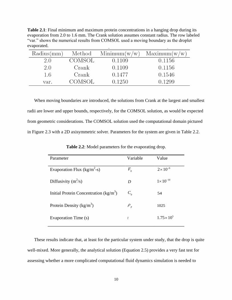
Table 2.1: Final minimum and maximum protein concentrations in a hanging drop during its
evaporation from 2.0 to 1.6 mm. The Crank solution assumes constant radius. The row labeled
“var.” shows the numerical results from COMSOL used a moving boundary as the droplet
evaporated.
When moving boundaries are introduced, the solutions from Crank at the largest and smallest
radii are lower and upper bounds, respectively, for the COMSOL solution, as would be expected
from geometric considerations. The COMSOL solution used the computational domain pictured
in Figure 2.3 with a 2D axisymmetric solver. Parameters for the system are given in Table 2.2.
Table 2.2: Model parameters for the evaporating drop.
Parameter Variable Value
Evaporation Flux (kg/m2-s) 0
F
62 10
Diffusivity (m2/s) D
101 10
Initial Protein Concentration (kg/m3) 0
C 54
Protein Density (kg/m3) p
1025
Evaporation Time (s) t 51.75 10
These results indicate that, at least for the particular system under study, that the drop is quite
well-mixed. More generally, the analytical solution (Equation 2.5) provides a very fast test for
assessing whether a more complicated computational fluid dynamics simulation is needed to
Page 14
11
determine whether the drop is well-mixed. The estimation of nucleation and growth kinetics
within drops is greatly simplified when the drop is well-mixed, and Equation 2.5 can be used to
redesign the operations to ensure well-mixedness. In particular, Equation 2.5 is affine in both the
flux and the drop radius. If it was desired to reduce the maximum concentration difference in the
drop by a factor of four, for example, this could be achieved by reducing the radius or the flux by
a factor 4, or by reducing both the radius and flux by a factor of 2.
Page 15
12
3 Ultrasound-Induced Breakage
3.1 Introduction
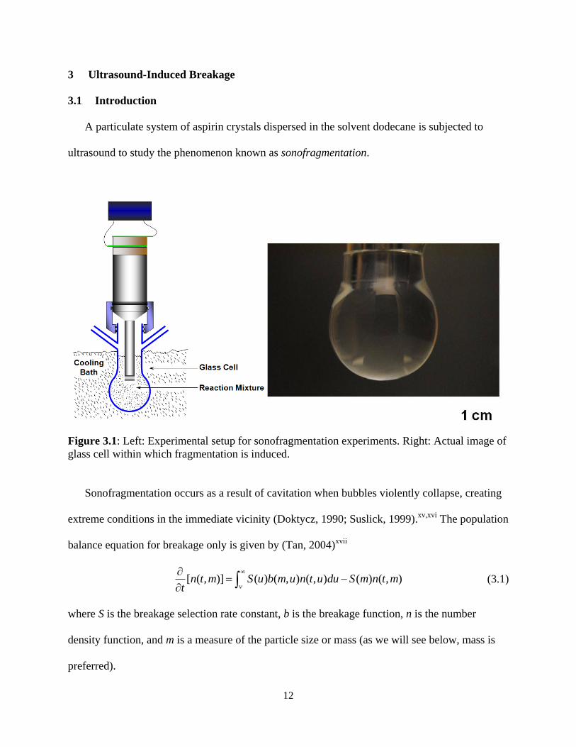
A particulate system of aspirin crystals dispersed in the solvent dodecane is subjected to
ultrasound to study the phenomenon known as sonofragmentation.
Figure 3.1: Left: Experimental setup for sonofragmentation experiments. Right: Actual image of
glass cell within which fragmentation is induced.
Sonofragmentation occurs as a result of cavitation when bubbles violently collapse, creating
extreme conditions in the immediate vicinity (Doktycz, 1990; Suslick, 1999).xv,xvi
The population
balance equation for breakage only is given by (Tan, 2004)xvii
[ ( , )] ( ) ( , ) ( , ) ( ) ( , )v
n t m S u b m u n t u du S m n t mt
(3.1)
where S is the breakage selection rate constant, b is the breakage function, n is the number
density function, and m is a measure of the particle size or mass (as we will see below, mass is
preferred).
Page 16
13
The selection rate constant S in Equation 3.1 is written as a function of particle mass as
1( ) , 0qS m S m q (3.2)
where S1 and q are parameters fitted to the experimental data. The exponent q is restricted to
non-negative values; large particles are more likely to come in contact with cavitation sites.
3.2 Methodsxviii
Intuitively, the selection rate constant is related to the cavitation rate by an efficiency factor.
Colussi et al. (1999)xix
and Son et al. (2009)xx
have reported that the rate of cavitation is
proportional to applied power (over the ranges discussed here). Experimentally, cavitation rate is
exponentially related to fluid viscosity.
Figure 3.2: Experimental data and model relationship for the effect of viscosity on cavitation.
The experimental data can therefore be combined using the following relationship.
1 0 exp( 0.0069 )S S (3.3)
0 200 400 6000
10
20
30
40
Viscosity (cSt)
Cavitation E
vents
model fit
experimental data
y=31.47exp(-0.006926x)
Page 17
14
Data from the above system are provided in the form of the measure of circularity and surface
area for a representative set of aspirin crystals. Circularity, c, is defined as
24c a p (3.4)
where a is the surface area and p is the perimeter of the 2D image of the particle (Figure 3.3).
Figure 3.3: SEM image of aspirin crystals synthesized in dodecane.
The crystal depth, d, (defined as the shortest dimension) is estimated from the surface area and
perimeter using a proportionality constant obtained from the SEM images assuming the particles
have a similar shape:
2.06
ad
p (3.5)
Finally, the mass for each particle can be calculated using the density, .
m ad (3.6)
Now a procedure is described that greatly reduces the computational cost in solving the
population balance for breakage. A minimum particle size, mmin, is chosen, and the data are
Page 18
15
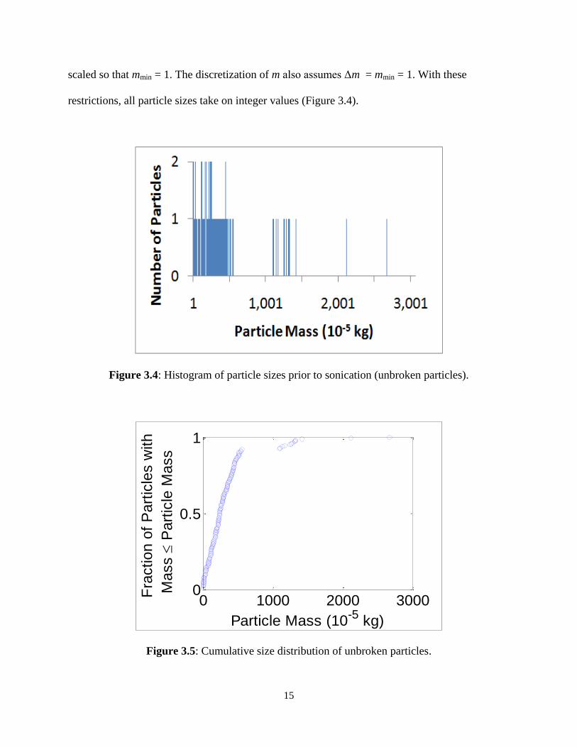
scaled so that mmin = 1. The discretization of m also assumes Δm = mmin = 1. With these
restrictions, all particle sizes take on integer values (Figure 3.4).
Figure 3.4: Histogram of particle sizes prior to sonication (unbroken particles).
Figure 3.5: Cumulative size distribution of unbroken particles.
0 1000 2000 30000
0.5
1
Particle Mass (10-5
kg)
Fra
ctio
n o
f P
art
icle
s w
ith
Ma
ss
Pa
rtic
le M
ass
Page 19
16
Figure 3.6: An equal, binary breakage model when particle sizes are restricted to integer values.
Assuming that particles break into two equally sized pieces for even integer sizes and one of
each for odd integer sizes (e.g., size 4 breaks into 2 and 2; size 5 breaks into 2 and 3), the
breakage function, b, in Equation 3.1 can be written as
2, 2
1, 2 1( , )
1, 2 1
0,
u m
u mb m u
u m
otherwise
(3.7)
Discretizing the population balance equation (Equation 3.1) spatially leads to
1 1
1 1
max
1 1
1 1
max
1
2 (2 ) ( , 2 ) (2 1) ( , 2 1), 1
2 (2 ) ( , 2 ) 2 1 ( ,2 1)1 /2
(2 1) ( , 2 1) ( ) ( , ),[ ( , )]
2 (2 ) ( , 2 ) (2 1) ( , 2 1)
( ) ( , ),
q q
i i i i
qq
i i i i
q q
i i i ii
q q
i i i i
q
i i
S m n t m S m n t m i
S m n t m S m n t mi i i
S m n t m S m n t mn t m
t S m n t m S m n t mi i
S m n t m
1 max max
/2
( ) ( , ), /2q
i iS m n t m i i i
(3.8)
The time derivative is replaced with the first-order forward-difference approximation
1( , ) ( , )
[ ( , )]j i j i
i
n t m n t mn t m
t t
(3.9)
with the initial condition determined by the „unbroken particles‟ CSD given by experimental
data. The combination of Equations 3.8 and 3.9 can produce negative values of mass for
Page 20
17
sufficiently high values of 0S and q. In order to prevent this error, a minimum function is
included with each coefficient for ( , )in t m . For example, in the case of 1i , the function takes
the form
1 1
1
( , ) ( , ) 2min 1,( ) (2 ) ( ,2 )
min 1,( ) (2 1) ( ,2 1)
q
j i j i i j i
q
i j i
n t m n t m t S m n t m
t S m n t m
(3.10)
The discretized population balance equations can be solved most quickly in Matlab by
writing the right-hand side of the expressions in Equation 3.8 as the multiplication of a sparse
matrix and a vector as shown in Equation 3.11.
1( ) ( )j jn t n t A (3.11)
where ( )jn t is a row vector of length maxi as defined above and A is a square matrix with an
interesting form. The 10 10 example of A is given below.
2 2
3 3 3
4 4
5 5 5
6 6
7 7 7
8 8
9 9 9
10 10
1 0 0 0 0 0 0 0 0 0
2 1 0 0 0 0 0 0 0 0
1 0 0 0 0 0 0 0
0 2 0 1 0 0 0 0 0 0
0 0 1 0 0 0 0 0
0 0 2 0 0 1 0 0 0 0
0 0 0 0 1 0 0 0
0 0 0 2 0 0 0 1 0 0
0 0 0 0 0 0 1 0
0 0 0 0 2 0 0 0 0 1
A
(3.12)
The values of i are the coefficients for ( , )in t m given in Equation 3.10. The matrix A consists of
entries along the main diagonal (slope = –1) and a diagonal band, 3 entries wide, with a slope of
–2. The matrix can be defined as sparse in order to provide computation speedup and decrease
the memory requirement.
Page 21
18
An alternative breakage model is now introduced, whereby instead of an equal, binary
breakage event, each particle breaks into a uniform distribution (by number) of each particle size
smaller than the parent particle. The matrix analogous to A described above is
2 2 2
3 3 3 3 3
4 4 4 4 4 4 4
5 5 5 5 5 5 5 5 5
6 6 6 6 6 6 6 6 6 6 6
7 7 7 7 7 7 7 7 7 7 7 7 7
8 8 8 8 8 8 8 8 8 8 8 8 8 8 8
9 9 9 9
1 0 0 0 0 0 0 0 0 0
2 1 0 0 0 0 0 0 0 0
1 0 0 0 0 0 0 0
2 1 0 0 0 0 0 0
1 0 0 0 0 0
2 1 0 0 0 0
1 0 0 0
2 1 0 0
B
9 9 9 9 9 9 9 9 9 9 9 9 9
10 10 10 10 10 10 10 10 10 10 10 10 10 10 10 10 10 10 10
1 0
2 1
(3.13)
In matrix B, the values i are the same as defined above. Assuming each integer breakage is
equally probable, the parameter i ensures an overall conservation of mass.
2, even
1
2, odd
i
ii
ii
(3.14)
Either model provides a solution for given values of the two parameters, S0 and q, which can be
compared to the experimental data by converting the results into cumulative size distributions,
Fmodel and Fexp (the use of cumulative distributions avoids the binning errors that arise when
histograms are used to approximate distributions). Under the assumption of additive independent
measurement errors, the maximum-likelihood and minimum-variance parameters based on
Riemann-sum approximation of the integral-form for the squared error satisfy the expression
2
2 model exp
1min , ; ,
j i j i j ii j ij
F t m F t m t m
(3.15)
Page 22
19
Assuming the σij are all the same, the Δtj are all the same, and setting Δmi = 1 which weighs
masses more heavily where more data points have been collected, and E equal to the difference
between the model and experimental cumulative distributions, the expression can be simplified
to
2min min T
ij iji j i j
R E E E
(3.16)
Matlab is inherently slow when dealing with loops and fast when using matrix-vector arithmetic.
The above objective can be computed in Matlab as a single function call to the Frobenius norm
of the matrix E, or the elements of the matrix E can be stacked as a long vector and the objective
computed using the vector 2-norm or vector-vector multiply commands.
Beck and Arnold present one method for constructing a confidence interval for the
parameters using the F distribution:xxi
1 ( , )/( )
S RF p n p
R n p (3.17)
(S , the sum-of-squared error, is the objective function of the optimization in Equation 3.16, n
is the number of data points, p is the number of parameters, and 1 is the confidence level for
the region.
3.3 Results
The parameters (assuming equal, binary breakage) were estimated from the experimental
data from 1-minute trials using aspirin in dodecane for 6 different levels of ultrasonic power (3,
5, 10, 20, 30, and 40 W).
Page 23
20
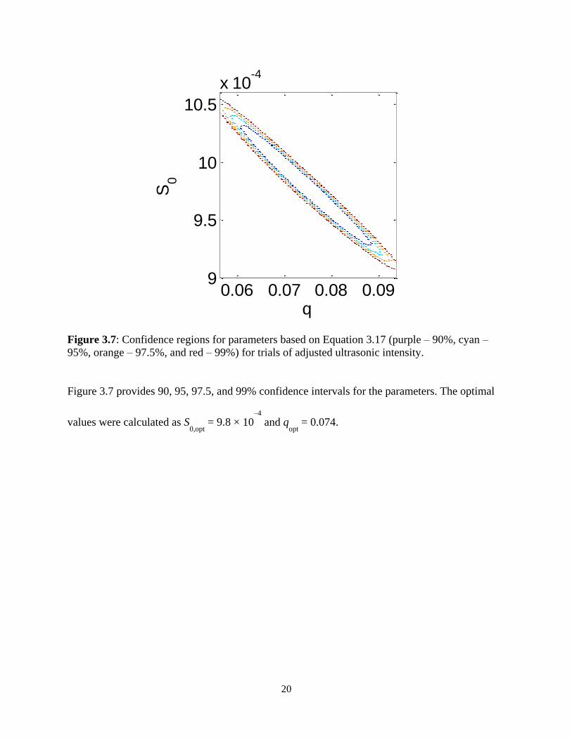
Figure 3.7: Confidence regions for parameters based on Equation 3.17 (purple – 90%, cyan –
95%, orange – 97.5%, and red – 99%) for trials of adjusted ultrasonic intensity.
Figure 3.7 provides 90, 95, 97.5, and 99% confidence intervals for the parameters. The optimal
values were calculated as S0,opt
= 9.8 × 10⁻⁴
and q
opt = 0.074.
q
S0
0.06 0.07 0.08 0.099
9.5
10
10.5
x 10-4
Page 24
21
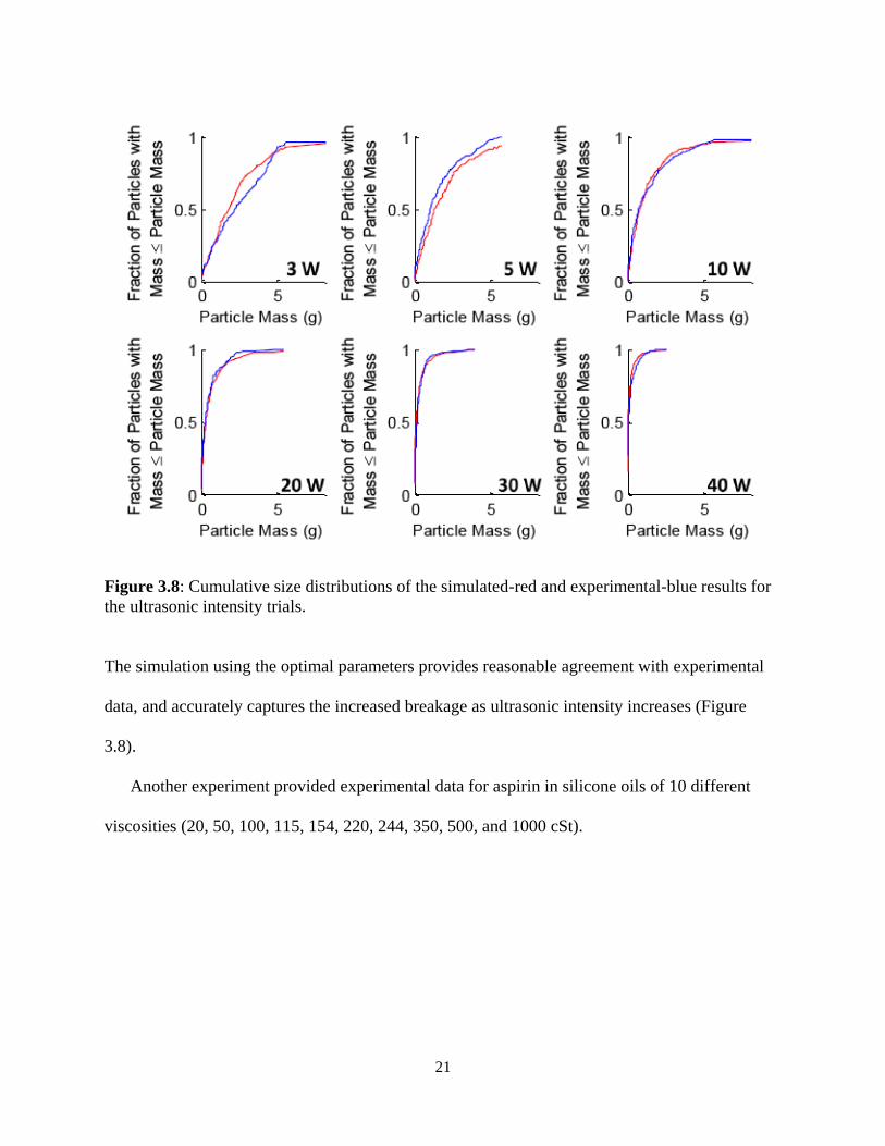
Figure 3.8: Cumulative size distributions of the simulated-red and experimental-blue results for
the ultrasonic intensity trials.
The simulation using the optimal parameters provides reasonable agreement with experimental
data, and accurately captures the increased breakage as ultrasonic intensity increases (Figure
3.8).
Another experiment provided experimental data for aspirin in silicone oils of 10 different
viscosities (20, 50, 100, 115, 154, 220, 244, 350, 500, and 1000 cSt).
Page 25
22
Figure 3.9: Confidence regions for parameters based on Equation 1.17 (purple – 90%, cyan –
95%, orange – 97.5%, and red – 99%) for trials of adjusted fluid viscosity.
Figure 3.9 provides 90, 95, 97.5, and 99 % confidence intervals for the parameters. The optimal
values were calculated as S0,opt
= 8.8 × 10⁻³
and qopt
= 5.6 × 10⁻⁶
. As seen in the figure, for this
experiment, the value of q = 0 falls within the confidence regions indicating that the breakage
rate of 1D particles in viscous fluids is not size dependent for the given assumptions.
q
S0
0 0.5 1 1.5
x 10-3
8.6
8.795
8.99x 10
-4
Page 26
23
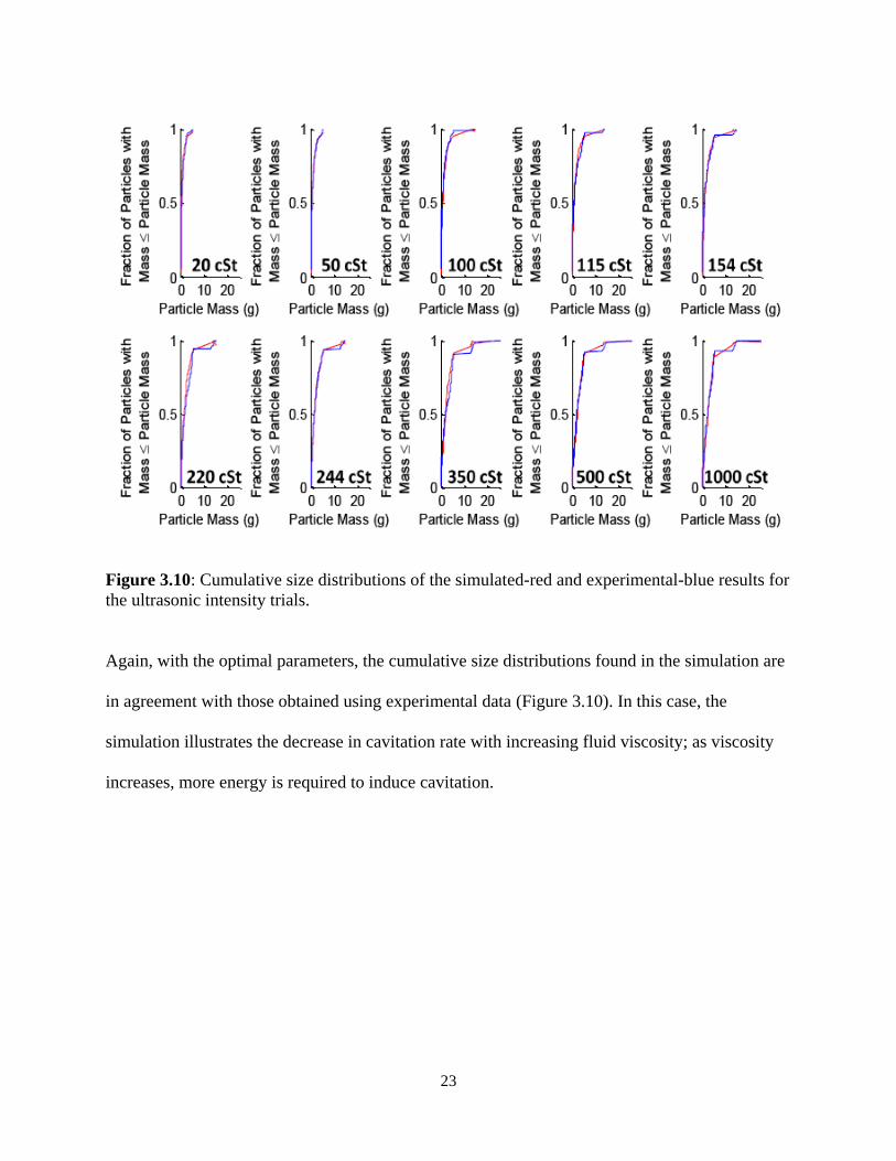
Figure 3.10: Cumulative size distributions of the simulated-red and experimental-blue results for
the ultrasonic intensity trials.
Again, with the optimal parameters, the cumulative size distributions found in the simulation are
in agreement with those obtained using experimental data (Figure 3.10). In this case, the
simulation illustrates the decrease in cavitation rate with increasing fluid viscosity; as viscosity
increases, more energy is required to induce cavitation.
Page 27
24
4 Fouling in Cooling Crystallization
4.1 Introduction
A well-known method to induce crystallization of most substances is cooling a liquid
solution in a jacketed reactor. The increased driving force for cooling at the reactor wall can
cause a buildup of unusable product due to heterogeneous crystallization with the wall. This
phenomenon is known as fouling, and over time, it can cause significant loss of product and
decreased cooling efficiency by creating additional resistance to heat transfer. Fouling has
become of relevance recently in the pharmaceuticals industry, as engineers have been working to
develop continuous-flow crystallizers that are able to address all of the key issues that commonly
arise when crystallizing organic molecules (e.g., polymorphism). An example in which fouling
prevented a continuous-flow crystallizer design from being effective was published rather
recently (Euhus, 2003).xxii
This paper builds on that of Woo et al. (2006) and Woo et al. (2009) who developed an anti-
solvent crystallizer model that combined computational fluid dynamics (CFD) with the full
solution to the population balance equation and a probability density function-based
micromixing model.xxiii, vii
The paper also builds on that of Brahim et al. (2003) who presented a
model for the fouling of surfaces during industrial heat transfer processes.xxiv
This simulation
investigates the effects of fouling on the crystallization yield and crystal size distribution (CSD)
of the product in a mixed crystallizer. Using the method presented by Brahim and the references
therein, fouling effects were added to a simplified version of the Woo model – the micromixing
model is not necessary for cooling crystallization – for the simulation of paracetamol
crystallizing in a mixture of acetic acid and water.
A population balance equation for spatially inhomogeneous crystallization is
Page 28
25
0
( , , ) ( )( , , ) ) ( , , )
i i it i i
i i ii i i i
G r c T f v ff fD B f c T r r h f c T
t r x x x
(4.1)
where f is the number distribution of crystal sizes,iG is the growth in the internal coordinate,
ir ,
c is the concentration, and T is the temperature. The spatial inhomogeneity results in the second
summation where the velocity,iv , is a change in the external coordinate,
ix , andtD is the
turbulent diffusivity. Generation and consumption terms are included as primary nucleation, B ,
and secondary nucleation/attrition, h . is the Dirac delta function. Discretization with respect to
the internal coordinate and expressing on a mass basis givesxxiii
3. ,
.
4 4
1/2 1/2 1/2 1/2 1 1 ( 0)
( )
( ) ( ) ( ) ( )4 2 2
i w j w j
w j t
i i i i
c vj j j j r j j j r j j
v f fdf D
dt x x x
k r rr r G f f G f f B
r
(4.2)
where ,w jf is the cell-averaged crystal mass in a cell centered at rj, jf is the corresponding cell-
averaged number density, and ( )r jf are the minmod approximated derivatives of the number
density. The crystal density,c , and shape factor,
vk , relate the number and mass distributions.
The equation can be solved simultaneously with the equations of momentum, energy, continuity,
and turbulence.
The nucleation rate, B , is given in units of (number of nuclei)/(m3s) by Granberg et al.
(1999):xxv
3
8 3
2
ln
8.56080 10 exp 1.22850 10 , 0
ln
c
v
m
m
cB c
c
c
(4.3)
Page 29
26
where c is the crystal density in kg/m3,
mc is the supersaturated solute concentration in units of
(kg solute)/(kg solvent), and m mc c c is the degree of supersaturation (note: 0B for
0c ). The solubility, x, in terms mass fraction of solute is given as a function of temperature
by Grant et al. (1984):xxvi
0 1log( ) log( ) log( )
2.3
pcHx T C A B T C
RT R T
(4.4)
For paracetamol in water, A = −12200, B = 49.69, and C = −330.4. The solubilities, mc, in terms
of (kg solute)/(kg solvent), and vc, in terms of (kg solute)/m
3, can be found by the relationships:
1
pa
m
w
MWxc
x MW
(4.5)
55.61
v pa
xc MW
x
(4.6)
The paracetamol growth rate, G (m/s) isxxiii
2 2 4
1 16
a d i iv v
v c i d d
k k k kG c c
k k k k
(4.7)
where ki and kd are kinetic rate constants for the solute incorporation into and diffusion to the
crystal surface, ka and kv are area and volume shape factors, and v v vc c c is the degree of
supersaturation of paracetamol on a volume basis (kg solute/m3).
The heterogeneous crystallization can be described as the growth of a fouling layer along the
walls of the reactor.xxiv
The thickness of the fouling layer is given by
f
f
mx
(4.8)
where f is the density of the fouling layer ( f c ) and m is the total mass deposited:
Page 30
27
,d r
mm m
t
(4.9)
The mass deposition rate, dm , is defined in terms of the growth rate above.
d cm G (4.10)
The mass removal rate, rm , is given by Bohnet (1987)xxvii
2 1/3 2(1 ) ( )r f p f
Km T d g x v
P (4.11)
where T is the temperature difference across the fouling layer, is the coefficient of linear
expansion for the fouling layer, dp is the mean crystal diameter, and are the density and
viscosity of the solution, respectively, and v is the velocity of the flowing solution at the surface
of the fouling layer. The cohesion coefficient P/K given by Krause (1993):xxviii
4.2 Methods
The simulation was performed using the Fluent software (Fluent 6.3.26) to solve the
equations given above for the cylindrical agitated tank shown below (Figure 4.1).
Page 31
28
Figure 4.1: Computational domain for cylindrical agitated tank (rotated 90 degrees clockwise).
The segment AK is the axis of symmetry, segment GS is a computational border only (not a
physical border), and the region F4 represents the impeller blade. The points are given in units of
meters.
The evolution of the particle size distribution is shown in Figure 4.2. The PSD rapidly
changes when the seeds are first placed in the supersaturated solution. After one minute, rapid
growth has slowed, and the crystals growth decreases further as the degree of supersaturation
decreases. The velocity profile in the tank reaches a steady state within one minute (Figure 4.3).
The temperature profile within the tank continues to evolve as scales grow along the reactor
interior surfaces.
Page 32
29
Figure 4.2: The evolution particle size distribution observed in simulation of an
agitated tank with fouling along the reactor walls.
Figure 4.3: Velocity profiles simulated in the agitated tank for 1, 10, 60, and 1800 seconds).
0.00E+00
5.00E+07
1.00E+08
1.50E+08
2.00E+08
2.50E+08
3.00E+08
0 100 200 300 400
nu
mb
er/m
icro
n-L
iter
size (microns)
10 seconds
1 minute
5 minutes
30 minutes
Page 33
30
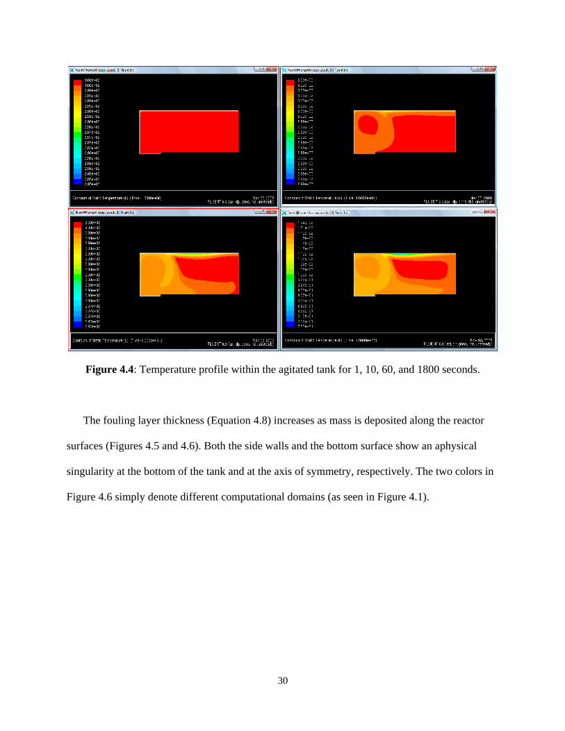
Figure 4.4: Temperature profile within the agitated tank for 1, 10, 60, and 1800 seconds.
The fouling layer thickness (Equation 4.8) increases as mass is deposited along the reactor
surfaces (Figures 4.5 and 4.6). Both the side walls and the bottom surface show an aphysical
singularity at the bottom of the tank and at the axis of symmetry, respectively. The two colors in
Figure 4.6 simply denote different computational domains (as seen in Figure 4.1).
Page 34
31
Figure 4.5: Fouling layer thickness (m) along the bottom of the tank after 10 and 60 seconds.
Figure 4.6: Fouling layer thickness (m) along the tank side walls after 10 and 60 seconds.
Page 35
32
5 Future Work
The eventual goal of my research is to combine the ideas developed during the projects
discussed in the previous chapters to create simulations for the modeling of the crystallization
phenomena and interactions with the fluid dynamics to the level of computational efficiency and
model fidelity so that the simulations can be used in the design of industrial-scale crystallizers. I
will integrate first-principles models for secondary nucleation, aggregation/agglomeration, and
breakage and will replace the pseudo-homogeneous assumption of Woo (2006)xxiii
with a
multiphase model.
While very detailed first-principles models of the individual phenomena can be developed,
the simulation of the most sophisticated models of such phenomena is too computationally
expensive to solve within each grid cell of a computational fluid dynamics
macromixing/micromixing simulation. So hypotheses will be made as to which simplifying
assumptions will reduce computational cost while minimizing the loss in numerical accuracy for
all critical variables in the overall simulation. These hypotheses will be tested both by scaling
analysis and by comparing the corresponding simulations to detailed simulations of each
individual phenomenon (such as aggregation) in isolation. This will enable me to rule out
hypotheses that lack sufficient fidelity. The simulation equations for each phenomenon with the
best trade-off between computational efficiency and numerical accuracy will be incorporated
into the overall simulation of macromixing and micromixing to simulate all of the crystallization
phenomena and the fluid dynamics simultaneously.
The expected results are a set of simulation codes that have an order-of-magnitude higher
fidelity than existing codes for simultaneously simulating crystallization phenomena and fluid
Page 36
33
dynamics in agitated vessels, while being computationally efficient enough for applications in
design of crystallization processes with improved product quality and consistency.
Page 37
34
6 Acknowledgments
First and foremost, I would like to thank my advisor Dr. Richard D. Braatz for his insights
and encouragement. Additionally, thanks to Brad Zeiger and Dr. Ken S. Suslick for providing the
experimental data in the ultrasonic breakage chapter and advice toward modeling. Thanks to the
rest of the Braatz group and my roommates for listening, giving suggestions, and asking the right
questions. Finally, thanks to my parents, siblings, and fiancée for their love and support.
Page 38
35
7 References i Mullin, J.W. Crystallization, 4
th ed., 2001, Elsevier, Oxford.
ii Wey, J.S., P.H. Karpinski, Handbook of Industrial Crystallization, 2
nd ed., Myerson, A.S.,
Editor, 2002, Boston, pp. 231-248.
iii Kitamura, M., Y. Hayashi, T. Hara, Effect of Solvent and Molecular Structure on the
Crystallization of Polymorphs of BPT esters, Journal of Crystal Growth, 2008, 310(12),
pp. 3067-71.
iv Kitamura, M. Crystallization and Transformation Mechanism of Calcium Carbonate
Polymorphs and the Effect of Magnesium Ion, Journal of Colloid and Interface Science,
2001, 236(2), pp. 318-27.
v U.S. Food and Drug Administration, Pharmaceutical cGMPs for the 21
st Century – A Risk
Based Approach, September 2004.
vi Woo X.Y, Modeling and Simulation of Anti-Solvent Crystallization: Mixing and Control,
Ph.D. Thesis, 2007, University of Illinois at Urbana-Champaign.
vii Woo X.Y., R.B.H. Tan, R.D. Braatz, Modeling and Computational Fluid Dynamics –
Population Balance Equation – Micromixing Simulation of Impinging Jet Crystallizers,
Crystal Growth & Design, 2009, 9(1), pp 156-164.
viii Goh, L.M., K. Chen, V. Bhamidi, G. He, N.C.S. Kee, P.J.A. Kenis, C.F. Zukoski, R.D.
Braatz, A Stochastic Model for Nucleation Kinetics Determination in Droplet-Based
Microfluidic Systems, Crystal Growth & Design, 2010, 10(6) pp. 2515-21.
ix Talreja, S., D.Y. Kim, A.Y. Mirarefi, C.F. Zukoski, P.J.A. Kenis, Screening and
Optimization of Protein Crystallization Conditions through Gradual Evaporation Using
a Novel
Page 39
36
Crystallization Platform, Journal of Applied Crystallography, 2005, 21(23), pp. 10537-
44.
x Grant, M.L., D.A. Saville, The Role of Transport Phenomena in Protein Crystal Growth,
Journal of Crystal Growth, 1991, 108, pp. 8-18.
xi Grant, M.L., D.A. Saville, Long-Term Studies on Tetragonal Lysozyme Crystals Grown
in Quiescent and Forced Convection Environments, Journal of Crystal Growth, 1995,
153, pp. 42-54.
xii Goh, L.M., Dynamic Analysis of Pharmaceutical and Biological Systems from the Nano-
to Microscale, M.S. Thesis, University of Illinois at Urbana-Champaign, 2007.
xiii Ostrach, S., Low Gravity Fluid Flows, Annual Review of Fluid Mechanics, 1982, 14, pp.
313-345.
xiv Crank, J., The Mathematics of Diffusion – 2
nd Edition, 1975, Oxford University Press,
NewYork.
xv Doktycz, S.J., K.S. Suslick, Interparticle Collisions Driven by Ultrasound, Science, 1990, 247,
pp. 1067-69.
xvi Suslick, K.S., Y. Didenko, M.M. Fang, T. Hyeon, K.J. Kolbeck, W.B. McNamara III, M.M.
Mdleleni, M. Wong, Acoustic Cavitation and Its Chemical Consequences, Philosophical
Transactions of the Royal Society of London A, 1999, 357, pp. 335-53.
xvii Tan, H.S., A.D. Salman, M.J. Hounslow, Kinetics of Fluidised Bed Melt Granulation IV.
Selecting the Breakage Model, Powder Technology, 2004, 143-144, pp. 65-83.
xviii All experimental data was provided by Brad Zieger and Dr. Ken S. Suslick in the Department
of Chemistry at the University of Illinois.
xix Colussi, A.J., H.M. Hung, M.R. Hoffmann, Sonochemical Degradation Rates of Volatile
Page 40
37
Solutes, Journal of Physical Chemistry A, 1999, 103, pp. 2696-99.
xx Son Y., M. Lim, J. Kim, Investigation of Acoustic Cavitation Energy in a Large-Scale
Sonoreactor, Ultrasonics Sonochemistry, 2009, 16, pp. 552-556.
xxi Beck J.V., K.J. Arnold, Parameter Estimation in Engineering and Science, 1977, Wiley.
xxii Euhus, D.D., Nucleation in Bulk Solutions and Crystal Growth on Heat-Transfer Surfaces
During Evaporative Crystallization of Salts Composed of Na2CO3 and Na2SO4, Ph.D.
Thesis, 2003, Georgia Institute of Technology.
xxiii Woo, X.Y., R.B.H. Tan, P.S. Chow, R.D. Braatz, Simulation of Mixing Effects in
Antisolvent Crystallization Using a Coupled CFD-PDF-PBE Approach, Crystal Growth
& Design,
2006, 6(6), 1291-1303.
xxiv Brahim, F., W. Augustin, M. Bohnet, Numerical Simulation of the Fouling Process,
International Journal of Thermal Sciences, 2003, 42, 323-334.
xxv Granberg, R.A., D.G. Cook, A.C. Rasmuson, Crystallization of Paracetamol in Acetone
Water Mixtures, Journal of Crystal Growth, 1999, 198/199, 1287-1293.
xxvi Grant, D.J.W., M. Mehdizadeh, A.H.-L. Chow, J.E. Fairbrother, Non-Linear van‟t Hoff
Solubility – Temperature Plots and Their Pharmaceutical Interpretation, International
Journal of Pharmaceutics, 1984, 18, 25-38.
xxvii Bohnet, M., Fouling of Heat Transfer Surfaces, Chemical Engineering Technology, 1987,
10(2), 113-125.
xxviii Krause, S., Fouling of Heat Transfer Surfaces by Crystallization and Sedimentation,
International Chemical Engineering, 1993, 33, 355-401.