Computational Fluid Dynamics and Process Co-simulation ...

Computational Fluid Dynamics and Process Co-simulation Applied to Carbon Capture

Technologies

Yang Fei

Submitted in accordance with the requirements for the degree of

Doctor of Philosophy

The University of Leeds

Energy Technology Innovation Initiative

School of Chemical and Process Engineering

September, 2015

http://www.google.co.uk/url?sa=t&rct=j&q=&esrc=s&frm=1&source=web&cd=1&cad=rja&uact=8&ved=0CCAQFjAA&url=http%3A%2F%2Fetii.leeds.ac.uk%2F&ei=ovL1U5qvEKLo7AaG9oFY&usg=AFQjCNGezxuoRRLH9dyvDicfLGTC8MdWiA&sig2=gVtYlpnWsRsfzq74LYIcUQ&bvm=bv.73231344,d.d2s

https://www.google.co.uk/url?sa=t&rct=j&q=&esrc=s&frm=1&source=web&cd=1&cad=rja&uact=8&sqi=2&ved=0CCAQFjAA&url=https%3A%2F%2Fwww.engineering.leeds.ac.uk%2Fchemical%2F&ei=fPL1U5m5GI7japLxgKgG&usg=AFQjCNFQegg28mOSB_KHETuueElXZtzpKg&sig2=tIf9MXvgF1IJMcxQ8Xk4Pg&bvm=bv.73231344,d.d2s

- i -

The candidate confirms that the work submitted is his own, except where

work which has formed part of jointly authored publications has been

included. The contribution of the candidate and the other authors to this

work has been explicitly indicated below. The candidate confirms that

appropriate credit has been given within the thesis where reference has

been made to the work of others.

The work performed in Chapter 6 of this thesis has been published in the

following publication:

Y. Fei, S. Black, J. Szuhánszki, L. Ma, D.B. Ingham, P.J. Stanger, M.

Pourkashanian, Evaluation of the potential of retrofitting a coal power plant

to oxy-firing using CFD and process co-simulation, Fuel Processing

Technology, 131 (2015) 45-58.

I developed the reduced order models in order to link the CFD predictions to

the process modelling and also developed the oxy-coal power plant process

model. Sandy Black and Janos Szuhanszki provided valuable assistance in

setting up the CFD models. Penelope Stange gave meaningful suggestions

on the process power plant. Lin Ma, Derek Ingham and Mohammed

Pourkashanian are supervisors who provided helpful guidance on the overall

direction and innovation for the research.

This copy has been supplied on the understanding that it is copyright

material and that no quotation from the thesis may be published without

proper acknowledgement.

The right of Yang Fei to be identified as Author of this work has been

asserted by him in accordance with the Copyright, Designs and Patents Act

1988.

© 2015 The University of Leeds and Yang Fei

- ii -

Acknowledgements

I would like to pass my thanks to Dr. Lin Ma for leading me the right way to

learn and understand the background of chemical engineering; you always

discussed with me so patiently on every academic or daily issue and helped

me find the right way to work out problems. I would like to express my

gratitude to Prof. Derek Ingham whose profound knowledge and kind

personality continuously inspired me and he was always ready to help me

with professional advices and experience. My sincere thanks should also go

to Dr. Kevin Hughes, who helped me with so many academic and software

issues. Thank you Prof. Mohamed Pourkashanian for always encouraging

me with a big smile and providing professional suggestions when I was

worried about the simulation results or the research progress. Thank you

Prof. Gale, for spending so much time and energy to offer me strong support

after the ETII team’s move to Sheffield. Also I would like to thank Sandy

Black and Alastair Clements for helping me with CFD simulations. Thank

Janos Szuhánszki for providing me the experimental data for the 250 kWth

combustion test facility in Chapter 4.

My best friend Wen-lei Luo in Leeds, I remember the first day when I came

to Leeds and it was you that picked me up at the train station in the midnight.

I would like to acknowledge the China Scholarship Council and ETII,

University of Leeds, for providing me with the financial support to perform

this research work. RWE npower is acknowledged for the MOPEDS

validation data. EPSRC is acknowledged for the meaningful support.

- iii -

Abstract

In the energy supply sector, coal will still remain as a dominate role in the

foreseeable future because: it is comparatively cheap and widely distributed

around the world and more importantly, carbon capture and storage (CCS)

technologies make it possible to depend on coal with almost zero emission

of carbon dioxide (CO2). CCS involves capturing and purifying CO2 from the

emission source and then sequestering it safely and securely to avoid

emission to the atmosphere. Both the post-combustion and the oxy-fuel

technologies can be applied to existing power plants for CCS retrofit.

Accurate prediction of the performance of a CCS plant plays an important

role in reducing the technical risk of future integration of CCS with existing

power plants. This research combines the fundamental computational fluid

dynamics (CFD) and system process simulation technologies so that an

efficient co-simulation strategy can be achieved.

A 250 kWth coal combustion facility combined with a CO2 post capture plant

is taken to test the conception of the CFD and process co-simulation

approach. The CFD models are employed to account for the combustion

facility and the predicted results on the outlet gas compositions,

temperatures and mass flow rates are used to generate reduced order

models to linked to the model for the PACT CO2 post capture plant so that a

pilot scale whole plant model is achieved and validations have been made

where it is possible.

Afterwards, the a large scale conventional air-coal firing power plant is taken

into investigation: the CFD models for the boiler and the process models for

the whole plant have been developed. Further, the potential of retrofitting

this power plant to oxy-firing is evaluated using a CFD and process co-

simulation approach. The CFD techniques are employed to simulate the coal

combustion and heat transfer to the furnace water walls and heat

exchangers under air-firing and oxy-firing conditions. A set of reduced order

models has been developed to link the CFD predictions to the whole plant

- iv -

process model in order to simulate the performance of the power plant under

different load and oxygen enrichment conditions in an efficient manner.

Simulation results of this 500 MWe power plant indicate that it is possible to

retrofit it to oxy-firing without affecting its overall performance. Further, the

feasible range of oxygen enrichment for different power loads is identified to

be between 25% and 27%. However, the peak temperature on the

superheater platen 2 may increase in the oxy-coal mode at a high power

load beyond 450 MWe.

- v -

Table of content

Acknowledgements ..................................................................................... ii

Abstract ....................................................................................................... iii

Table of content........................................................................................... v

List of Tables ............................................................................................ viii

List of Figures ............................................................................................ xi

Nomenclature ............................................................................................ xv

Chapter 1. Introduction and Motivation ............................................... 1

1.1 Energy consumption and the role of coal ...................................... 1

1.2 Coal combustion and its impacts on the environment ................... 4

1.2.1 Coal combustion in conventional power stations................... 4

1.2.2 Impacts on the environment .................................................. 6

1.3 Carbon capture technologies ........................................................ 8

1.3.1 Pre-combustion ..................................................................... 9

1.3.2 Post-combustion ................................................................. 10

1.3.3 Oxy-fuel combustion ........................................................... 11

1.4 Power generation system modelling ........................................... 12

1.5 Research aims, novelties and scope of the thesis ...................... 14

1.5.1 Research aims and novelties .............................................. 14

1.5.1 Scope of the thesis .............................................................. 15

Chapter 2. Literature Review .............................................................. 17

2.1 Coal combustion process modelling ............................................ 17

2.1.1 Evaporation and devolatilisation .......................................... 18

2.1.2 Volatile combustion ............................................................. 20

2.1.3 Char combustion ................................................................. 22

2.1.4 Pollutant formation .............................................................. 24

2.2 Heat transfer and turbulence ....................................................... 26

2.2.1 Heat transfer ....................................................................... 27

2.2.2 Turbulence .......................................................................... 30

2.3 Carbon capture process modelling .............................................. 34

2.3.1 Chemical absorption process modelling .............................. 35

2.3.2 Oxy-coal combustion process modelling ............................. 41

2.3.3 CFD and process co-modelling activities ............................ 42

- vi -

2.4 Summary ..................................................................................... 44

Chapter 3. Experimental Facilities and Data ..................................... 45

3.1 The 250 kWth Combustion Test Facility (CTF) ............................ 45

3.1.1 Facility introduction ............................................................. 45

3.1.2 Burner description ............................................................... 46

3.1.3 Measurements .................................................................... 47

3.1.4 Fuel specification ................................................................ 48

3.1.5 Experimental settings .......................................................... 50

3.2 The PACT amine capture plant ................................................... 52

3.3 Didcot-A power plant ................................................................... 54

3.3.1 Configurations of the power plant ........................................ 54

3.3.2 Fuel specification ................................................................ 55

3.3.3 Boiler description ................................................................. 56

3.3.4 Boundary conditions and available data for the boiler ......... 57

3.4 Summary ..................................................................................... 60

Chapter 4. Modelling and Simulation of a Pilot Scale CO2 Capture System ................................................................................. 61

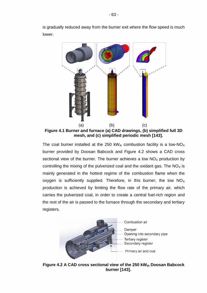
4.1 CFD modelling of the 250 kWth air-coal combustion test facility .......................................................................................... 62

4.1.1 Numerical set-up ................................................................. 62

4.1.2 Model validation .................................................................. 66

4.1.3 Simulation results and reduced order models ..................... 69

4.2 Integrated CFD and process modelling of the PACT facility........ 72

4.2.1 The gCCS system modelling environment .......................... 72

4.2.2 Model validation .................................................................. 74

4.2.3 The integration of the reduced order models into the process modelling and model settings ................................ 82

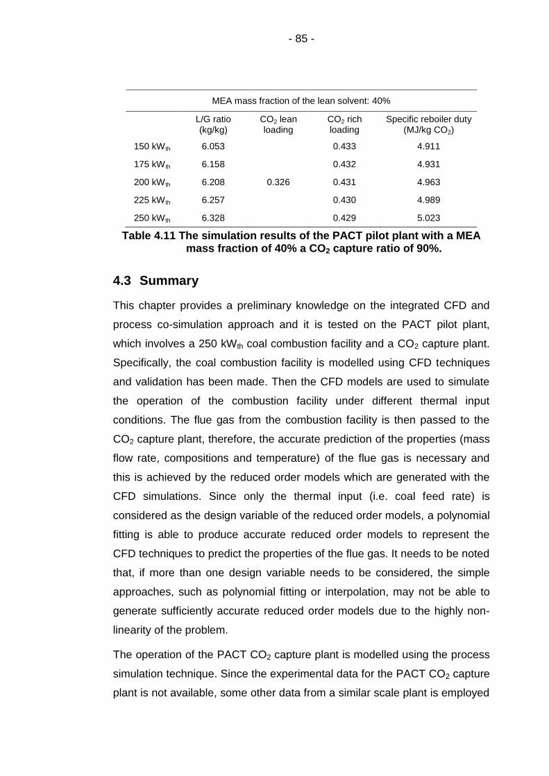
4.2.4 Simulation results of the PACT facility ................................ 82

4.3 Summary ..................................................................................... 85

Chapter 5. Modelling and Simulation of a Large-scale Power Plant ................................................................................................... 87

5.1 CFD modelling of the full-scale coal fired boiler .......................... 87

5.1.1 Model settings ..................................................................... 87

5.1.2 Coal data and boundary conditions ..................................... 90

5.1.3 Air-coal results and validation ............................................. 93

5.1.4 Air-coal and oxy-coal results analysis ................................. 94

5.1.5 Summary ............................................................................. 98

- vii -

5.2 The power plant simulations ........................................................ 98

5.2.1 Full plant description ........................................................... 99

5.2.2 Model components for the power plant ............................. 102

5.2.3 Air-coal firing results and validation ................................... 112

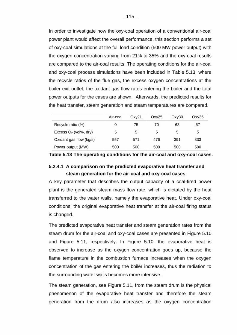
5.2.4 Air-coal and oxy-coal firing results analysis ...................... 114

5.3 Conclusions and limitations ....................................................... 119

Chapter 6. Evaluation of the Potential of Retrofitting a Coal Power Plant to Oxy-firing Using CFD and Process Co-Simulation ........................................................................................ 122

6.1 Research background ............................................................... 122

6.2 Essential component models for the co-simulation of the whole plant ................................................................................ 124

6.2.1 The natural circulation model ............................................ 125

6.2.2 The radiative heat exchanger model ................................. 126

6.2.3 The furnace model ............................................................ 127

6.3 The ROM development ............................................................. 128

6.3.1 Kriging interpolation .......................................................... 128

6.3.2 Design of experiments (DOE) for the ROM development . 130

6.3.3 The obtained ROMs .......................................................... 137

6.3.4 Validation of the ROMs ..................................................... 140

6.4 Model validation and discussions on the whole plant co-simulations ................................................................................ 141

6.4.1 Validation of the integrated CFD/process full plant model ................................................................................ 141

6.4.2 Results and discussions .................................................... 142

6.5 Conclusions ............................................................................... 149

Chapter 7. Summary and the recommended work for f ................. 150

7.1 Summary ................................................................................... 150

7.2 Future work ............................................................................... 154

List of References ................................................................................... 156

- viii -

List of Tables

Table 3.1 The El-Cerrejon coal analysis. ................................................. 49

Table 3.2 Parameters for Rosin-Rammler distribution. .......................... 49

Table 3.3 Operating conditions for the air-coal experiments. ............... 50

Table 3.4 The parameters for the absorber and the stripper columns. ............................................................................................ 52

Table 3.5 Essential components and instructions for the full plant. .... 55

Table 3.6 The Pittsburgh 8 coal analysis ................................................ 55

Table 3.7 Coal combustion properties of Pittsburgh 8. ......................... 56

Table 3.8 Flow split fractions and swirl angels of the burners. ............ 57

Table 3.9 Swirl directions of the burners. ............................................... 57

Table 3.10 Air-coal boundary conditions for the boiler at full load condition. ........................................................................................... 58

Table 3.11 Heat transfer to different heat exchangers of the boiler at full load condition for the air-coal case obtained from MOPEDS. ........................................................................................... 58

Table 3.12 The gas and steam temperatures of the main heat exchangers obtained by MOPEDS. .................................................. 59

Table 3.13 The steam generation rate, pressure and steam pressure of the steam drum obtained by MOPEDS. ...................... 59

Table 3.14 The steam flows, pressures, temperatures and power outputs from the steam turbines obtained by MOPEDS. ............... 59

Table 4.1 Sub-models used in the CFD modelling of the 250 kWth coal combustion facility. .................................................................. 65

Table 4.2 The predicted outlet mass fractions, temperatures and the mass flow rates of the flue gas at different thermal inputs. .... 70

Table 4.3 The components and mass fractions assumed in the flue gas. ............................................................................................. 71

Table 4.4 The test conditions of the absorber column in the tests 32 and 47. (The values in the brackets have been adjusted.)........ 75

Table 4.5 The validation results for the test 32. (The values in the brackets have been adjusted.) ......................................................... 76

Table 4.6 The validation results for the test 47. (The values in the brackets have been adjusted.) ......................................................... 77

Table 4.7 The input conditions of the stripper column in the tests 32 and 47. ........................................................................................... 78

Table 4.8 The considered thermal inputs and the corresponding mass flow rate and temperature of the flue gas. ............................ 83

- ix -

Table 4.9 The simulation results of the PACT pilot plant with a MEA mass fraction of 30% and a CO2 capture ratio of 90%. ......... 84

Table 4.10 The simulation results of the PACT pilot plant with a MEA mass fraction of 35% and a CO2 capture ratio of 90%. ......... 84

Table 4.11 The simulation results of the PACT pilot plant with a MEA mass fraction of 40% a CO2 capture ratio of 90%.................. 85

Table 5.1 Sub-models used in the CFD modelling of the boiler. ........... 89

Table 5.2 Pittsburgh 8 coal analysis. ....................................................... 91

Table 5.3 Operating parameters for the air and oxy-coal cases. .......... 91

Table 5.4 Average steam temperatures in the tube banks. ................... 92

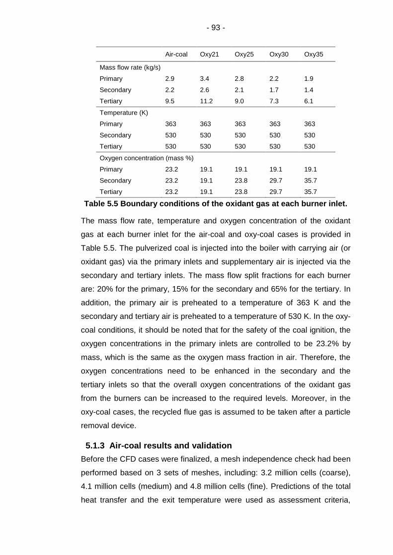
Table 5.5 Boundary conditions of the oxidant gas at each burner inlet. .................................................................................................... 93

Table 5.6 Heat transfer from the in-house code and the prediction from CFD for the air-coal case in the full-scale utility boiler. ........ 94

Table 5.7 Essential components and simple instructions for the full plant model. ............................................................................... 100

Table 5.8 PI/PID controllers used in the full plant model. .................... 101

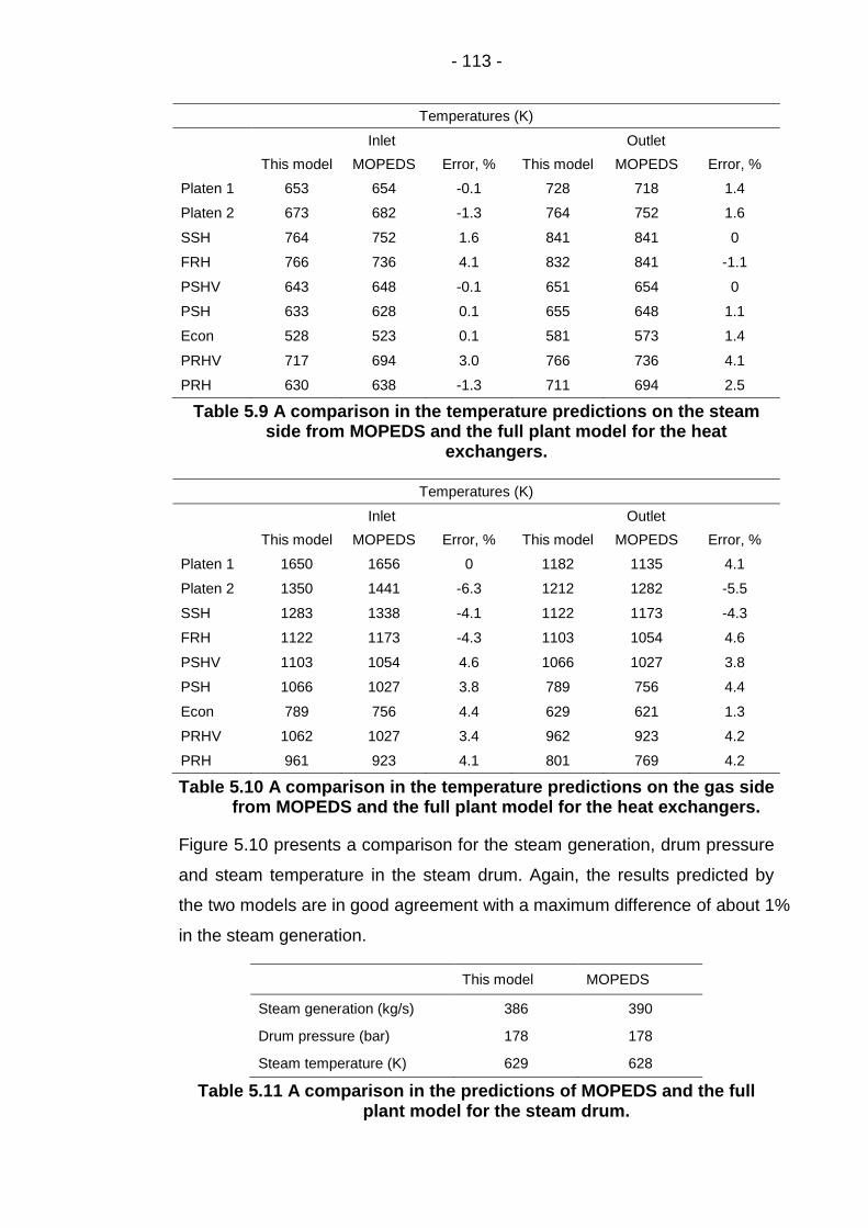
Table 5.9 A comparison in the temperature predictions on the steam side from MOPEDS and the full plant model for the heat exchangers. ............................................................................. 113

Table 5.10 A comparison in the temperature predictions on the gas side from MOPEDS and the full plant model for the heat exchangers. ..................................................................................... 113

Table 5.11 A comparison in the predictions of MOPEDS and the full plant model for the steam drum. ............................................. 113

Table 5.12 A comparison in the temperature and pressure predictions of MOPEDS and the full plant model for steam turbines (values in brackets are the MOPEDS results). ............... 114

Table 5.13 The operating conditions for the air-coal and oxy-coal cases. ............................................................................................... 115

Table 6.1 Operating conditions of the sampling points for the CFD simulations of the furnace. ............................................................ 132

Table 6.2 Boundary settings for the operating burners at 31.7kg/s coal input rate. ................................................................................. 132




- x -


Table 6.7 Heat transfer and furnace exit temperature predictions from the boiler CFD simulations. ................................................... 136

Table 6.8 Coal feed rates and oxygen concentrations of the validation cases. ............................................................................. 140

Table 6.9 Comparisons of heat transfer and temperature predictions between the CFD and ROMs. ..................................... 140

Table 6.10 A comparison in the temperature predictions on the steam side from MOPEDS and the full plant model for the heat exchangers. ............................................................................. 141

Table 6.11 A comparison in the temperature predictions on the gas side from MOPEDS and the full plant model for the heat exchangers. ..................................................................................... 142

Table 6.12 A comparison in the predictions of MOPEDS and the full plant model for the steam drum. ....................................... 142

- xi -

List of Figures

Figure 1.1 World energy consumption by fuel [3]. ................................... 2

Figure 1.2 Fuel used in electricity generation in the UK over the last 15 years [1]. .................................................................................. 2

Figure 1.3 Schematic of a coal fired sub-critical power plant. ................ 4

Figure 1.4 Coal burner in a furnace in a power station [6]. ..................... 5

Figure 1.5 Global CO2 emissions since 1900 [7]. ..................................... 7

Figure 1.6 Average atmospheric CO2 concentration since 1900 [7]....... 7

Figure 1.7 Sea level rise over the last 100 years [8]. ................................ 7

Figure 1.8 A simplified diagram for the pre-combustion process [16]. ....................................................................................................... 9

Figure 1.9 A simplified block diagram for the post-combustion process [16]. ...................................................................................... 10

Figure 1.10 A simplified block diagram for the oxy-fuel combustion process [16]. ................................................................. 12

Figure 2.1 Schematic of the combustion process of a coal particle [32]. ..................................................................................................... 17

Figure 2.2 A process flow diagram for CO2 capture using chemical absorption approach [117]. .............................................. 36

Figure 2.3 Descriptions of reactive absorption models with different abilities to describe the mass transfer and reaction kinetics [125]. .................................................................................... 38

Figure 3.1 Layout of the 250 kWth CTF and a CAD image of the furnace [143]. ..................................................................................... 45

Figure 3.2 Images of the Doosan Babcock 250 kWth coal burner [143]. (a) burner with the quarl; (b) disassembled view showing from top to bottom: damper for tertiary and secondary split, tertiary inner pipe, secondary inner pipe,

primary inner pipe, gas pipe; (c) assembled burner before installation and (d) burner installed in the CTF. ............................. 46

Figure 3.3 Sketch of the near burner region of the combustion rig. ..... 47

Figure 3.4 Images of the IFRF suction pyrometer showing the (a) rear view, and (b) front vi, showing radiation shield [143]. ........... 48

Figure 3.5 Images of a Medtherm GTW-50-24-21 584 heat probe [143]. ................................................................................................... 48

Figure 3.6 The fitted Rosin-Rammler curve [143]. .................................. 50

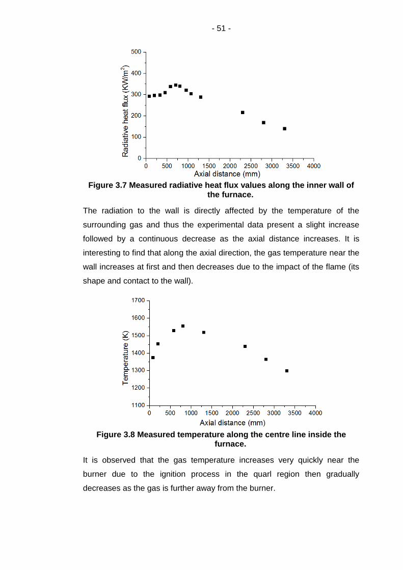
Figure 3.7 Measured radiative heat flux values along the inner wall of the furnace. ................................................................................... 51

- xii -

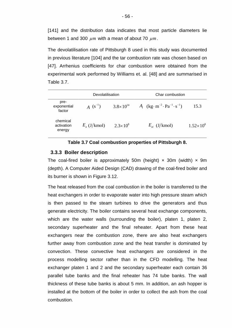
Figure 3.8 Measured temperature along the centre line inside the furnace. .............................................................................................. 51

Figure 3.9 Process flow diagram of the PACT amine capture plant [146]. ................................................................................................... 53

Figure 3.10 Configurations of the packing inside the absorber and stripper columns. .............................................................................. 53

Figure 3.11 Layout of the Didcot-A power plant. .................................... 54

Figure 3.12 A CAD drawing of the boiler and its burner. ....................... 57

Figure 4.1 Burner and furnace (a) CAD drawings, (b) simplified full 3D mesh, and (c) simplified periodic mesh [143]. .......................... 63

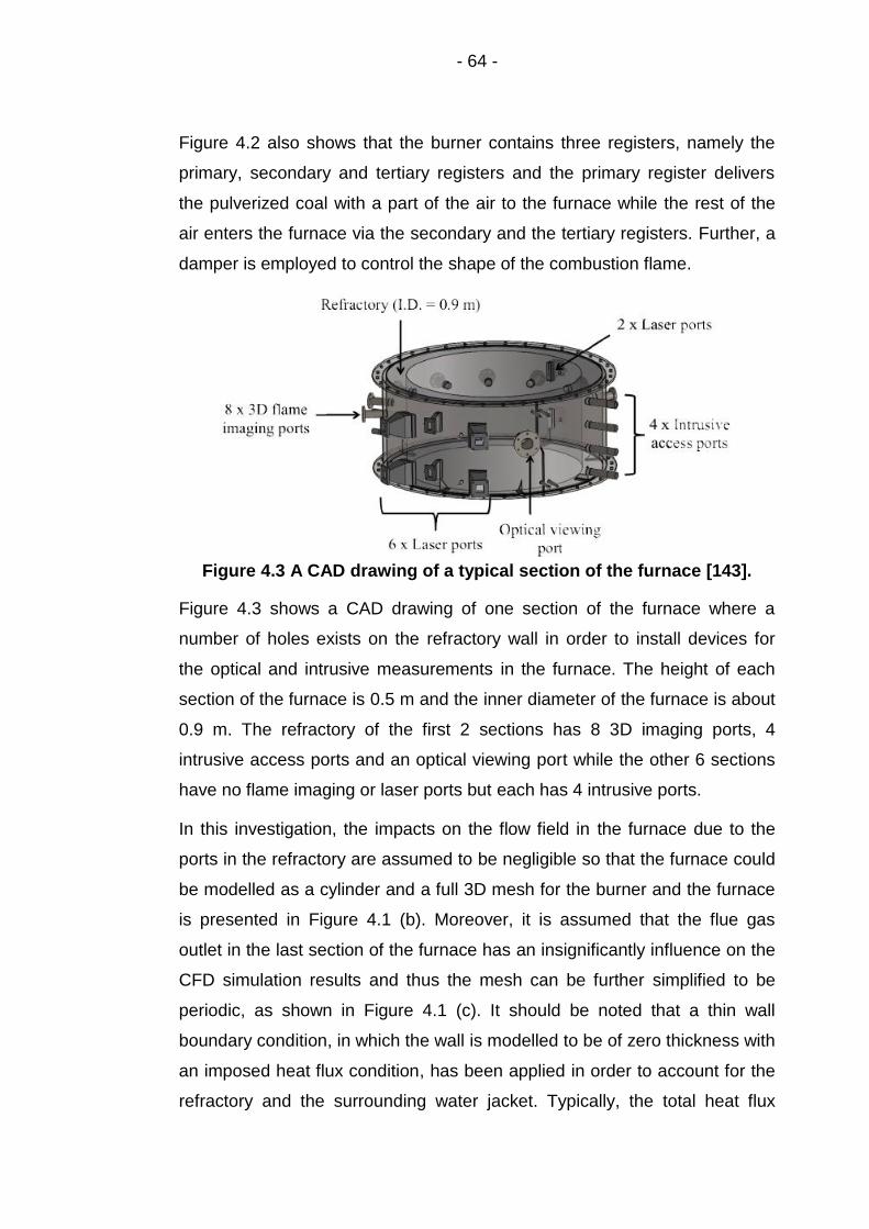
Figure 4.2 A CAD cross sectional view of the 250 kWth Doosan Babcock burner [143]. ...................................................................... 63

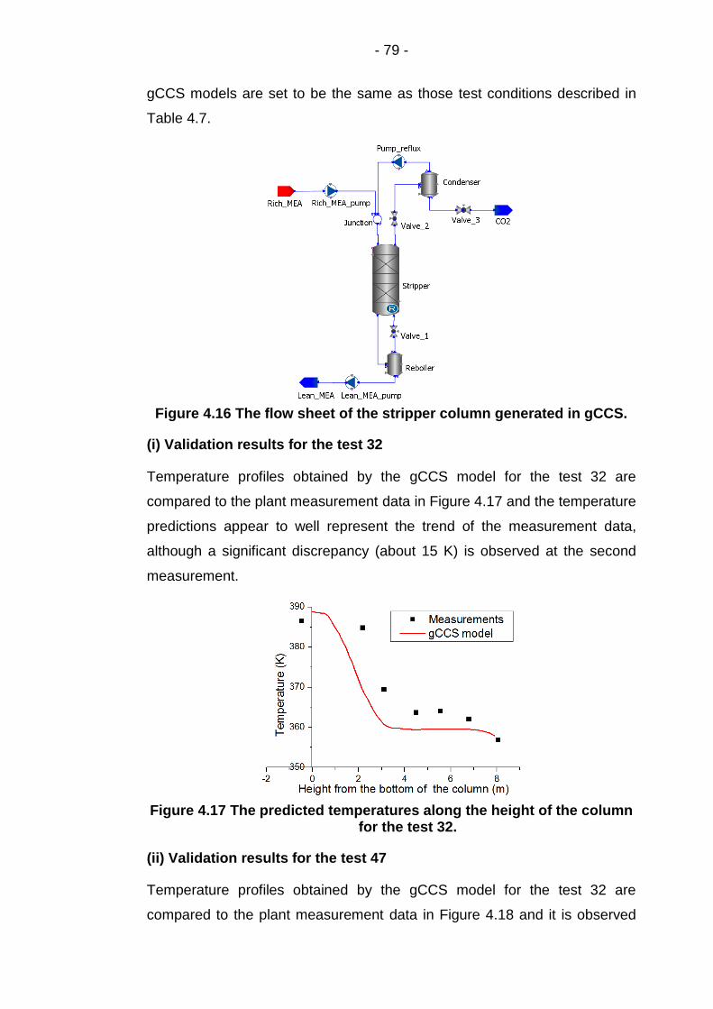
Figure 4.3 A CAD drawing of a typical section of the furnace [143]. .... 64

Figure 4.4 A predicted temperature distribution inside the furnace. .... 67

Figure 4.5 A plot of the temperatures along the centreline. .................. 68

Figure 4.6 A plot of the surface incident radiation along the wall. ....... 68

Figure 4.7 The predicted temperature profiles in the furnace with different thermal inputs. ................................................................... 70

Figure 4.8 The predicted velocity profiles in the furnace with different thermal inputs. ................................................................... 70

Figure 4.9 Temperature of the flue gas as a function of thermal input. .................................................................................................. 72

Figure 4.10 Mass flow rate of the flue gas as a function of thermal input. .................................................................................................. 72

Figure 4.11 Schematic representation of the two-film theory [158]. ..... 73

Figure 4.12 Absorber temperature measurement locations [167]......... 74

Figure 4.13 The flow sheet of the absorber column generated in gCCS. ................................................................................................. 76

Figure 4.14 The predicted temperatures along the height of the column for the test 32. ...................................................................... 77


Figure 4.16 The flow sheet of the stripper column generated in gCCS. ................................................................................................. 79



Figure 4.19 A flowsheet for the whole CO2 capture process in gCCS. ................................................................................................. 80

- xiii -

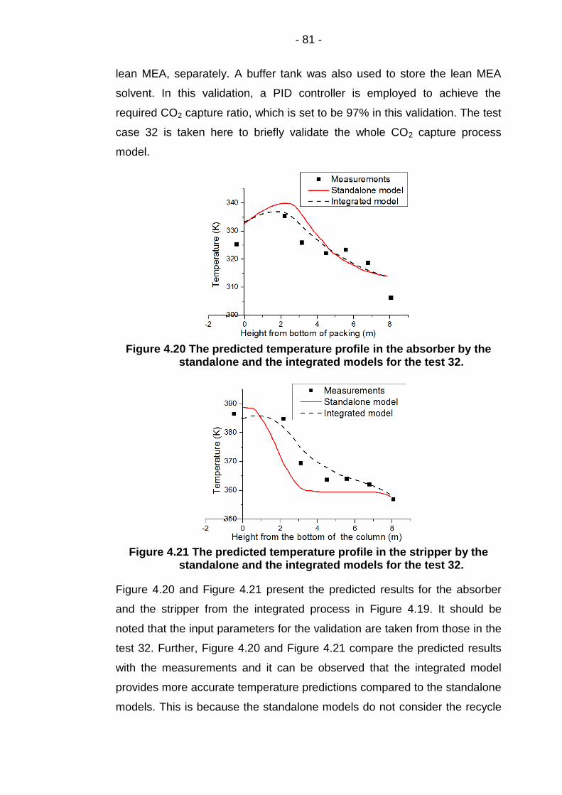
Figure 4.20 The predicted temperature profile in the absorber by the standalone and the integrated models for the test 32. ............ 81

Figure 4.21 The predicted temperature profile in the stripper by the standalone and the integrated models for the test 32. ............ 81

Figure 4.22 A flowsheet for the PACT amine plant generated in gCCS. ................................................................................................. 82

Figure 5.1 CFD mesh of the boiler (left) and its burner (right). ............. 88

Figure 5.2 Predicted temperature contours inside the boiler under air-coal and oxy-coal conditions. .................................................... 95

Figure 5.3 Predicted velocity contours inside the boiler under air-coal and oxy-coal conditions. .......................................................... 96

Figure 5.4 Predicted CO2 mole fraction profiles inside the boiler under air-coal and oxy-coal conditions. ......................................... 96

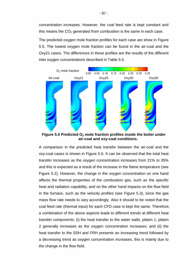
Figure 5.5 Predicted O2 mole fraction profiles inside the boiler under air-coal and oxy-coal conditions. ......................................... 97

Figure 5.6 Predicted heat transfer to different components under air-coal and oxy-coal conditions. .................................................... 98

Figure 5.7 A flowsheet of the virtually extended Didcot-A power plant, including the original Didcot-A power generating unit, an air separation unit and a CO2 compression unit. ..................... 99

Figure 5.8 A simplified thermal stage of a distillation column. ........... 104

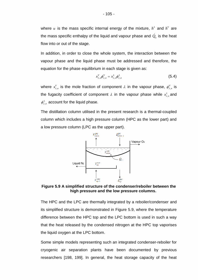
Figure 5.9 A simplified structure of the condenser/reboiler between the high pressure and the low pressure columns. ....... 105

Figure 5.10 Predicted evaporative heat transfer for the air-coal and oxy-coal cases. ........................................................................ 116

Figure 5.11 Predicted steam generation for the air-coal and oxy-coal cases. ....................................................................................... 116

Figure 5.12 Predicted total steam generation for the air-coal and oxy-coal cases................................................................................. 117

Figure 5.13 Predicted radiative heat transfer for the air-coal and oxy-coal cases. ................................................................................ 118

Figure 5.14 Predicted convective heat transfer for the air-coal and oxy-coal cases. ................................................................................ 118

Figure 5.15 Predicted steam temperatures at the inlet/outlet of the heat exchangers. ............................................................................. 119

Figure 6.1 Part of the predicted temperature contours inside the boiler. ............................................................................................... 136

Figure 6.2 ROMs for oxy-coal combustion of the boiler. ..................... 139

Figure 6.3 ROMs for the air-coal combustion of the boiler. ................ 139

Figure 6.4 The predicted evaporative heat as a function of oxygen concentration. ................................................................................. 143

- xiv -

Figure 6.5 The predicted steam generation as a function of the oxygen concentration. .................................................................... 144

Figure 6.6 The predicted steam generation as a function of the oxygen concentration. .................................................................... 144

Figure 6.7 The predicted radiative heat transfer as a function of the oxygen concentration. ............................................................. 145

Figure 6.8 The predicted convective heat transfer to the water/steam cycle as a function of oxygen concentration. ......... 146

Figure 6.9 Predicted steam temperatures at the inlet/outlet of the super heat components at 500MWe operation. ............................. 147

Figure 6.10 Predicted steam temperatures at the inlet/outlet of the super heat components at 400MWe operation. ............................. 147

Figure 6.11 Predicted peak temperatures on the tube wall. ................ 148

- xv -

Nomenclature

Abbreviations

ASU air separation unit

CAD computer-aided design

CBK carbon burnout kinetics

CCS carbon capture and storage

CFD computational fluid dynamics

Cov covariance

CPD chemical percolation devolatilisation

CPU CO2 compression and purification unit

CPU central processing unit

CTF combustion test facility

DNS direct numerical simulation

DOE design of experiments

DOM discrete ordinates method

DTM discrete transfer method

EDM eddy dissipation concept model

Eq equation

EDCM eddy dissipation concept model

ESP electrostatic precipitator

FG-DVC functional group-depolymerisation vaporization cross-linking

FGC flue gas condensation

FGD flue gas desulphurisation

FGR flue gas recycle

FRH final reheater

- xvi -

FSCK full spectrum correlated-k

HPC high pressure column

IGCC integrated gasification combined cycle

LBL line-by-line

LES large eddy simulation

LPC low pressure column

MEA monoethanolamine

MHT main heat exchanger

Mtoe million tonnes of oil equivalent

PACT pilot-scale advanced capture technology

PDF probability density function

Plat1 superheater platen 1

Plat2 superheater platen 2

PRH primary reheater

PSA pressure swing adsorption

RANS reynolds-averaged navier-stokes

PCA principal component analysis

ROM reduced order model

RSM reynolds stress model

RTE radiation transfer equation

SCR selective catalytic reduction

SGS sub-grid-scale

SNB statistical narrow band

SSH secondary superheater

SST shear stress transport

UDF user defined function

UKCCSRC United Kingdom carbon capture and storage research centre

- xvii -

WSGG weighted sum of gray gas

Latin alphabet

A effective heat transfer area 2m

a absorption coefficient 1 m

b dimensional scaling coefficients -

pC heat capacity J kg

F mass flow rate of the feed stream kg s

f number of degrees of freedom of the gas molecules -

f kernel function vector -

F response vector -

g gravity constant N kg

h mass specific enthalpy J kg

I radiation intensity 2W m

k turbulent kinetic energy in Section 2.2.2 2 2m s

k chemical reaction rate in Section 2.3.1 mol s

XRK an empirical constant describing the pressure drop -

L mass flow rate of the liquid kg s

m mass fraction -

M mass holdup kg

n refractive index -

p pressure Pa

Q heat, energy J

Q total heat flow J s

r position vector m

http://en.wikipedia.org/wiki/Degrees_of_freedom_(physics_and_chemistry)

- xviii -

r CO2 absorption rate mol s

R the correlation matrix -

s direction vector -

t time s

T temperature K

u velocity of the fluid in Chapter 2 m s

u mass specific internal energy in Chapter 5 J kg

V mass flow rate of the vapour in Section 5.2.2.1 kg s

V volume flow rate in Section 5.2.2.2 3m s

V volume in Sections 5.2.2.3, 5.2.2.4, 5.2.2.4 and 6.2.2 3m

W adiabatic power J s

x mole fraction in Section 5.2.2.2 -

y height of the riser m

Greek alphabet

geometry coefficient of the furnace -

β regression coefficient vector -

Kronecker delta

correlation parameter -

wavelength in Chapter 2 m

index of the components in Chapter 5 -

rate of dissipation of turbulent kinetic energy 2 2m s

adiabatic index of the gas -

Stefan-Boltzmann constant, 5.669X10-8 2 4/W m K in

Section 2.2.1

- xix -

square root of the process variance in Section 6.3.1 -

solid angle -

scattering phase function -

fugacity coefficient Pa

dynamic viscosity kg m s

density 3kg m

specific dissipation rate = k in Chapter 2 1 s

mass fraction in Chapter 6

mixed convection/radiation coefficient -

Subscripts

ad adiabatic flame

av average

circ circulation

d steam drum

eff effective

evap evaporative

gen electricity generator

dc downcomer

in inlet

liq liquid

mix mixture

out outlet

ox oxygen

R riser

ref reference

- xx -

s steam

sat saturation

tfr heat transfer

vap vapour

WDC water in the downcomer

w wall of the heat exchanger

XR water/steam mixture

- 1 -

Chapter 1. Introduction and Motivation

In this chapter, the motivation for this investigation is introduced. The

challenge of global warming and the necessity of using coal in the world

energy mix are discussed in Section 1.1 and the use of coal and its impacts

on the environment are analysed in Section 1.2. The solution for the

continuous use of coal while achieving a low carbon emission, namely, the

carbon capture and sequestration (CCS) technologies, are introduced in

Section 1.3. A brief introduction on power generation system modelling

techniques is presented in Section 1.4. Finally, the aims, novelties and the

scope of this thesis are outlined in Section 1.5.

1.1 Energy consumption and the role of coal

Investment shows that the world energy consumption will drastically

increase from 8,769 million tonnes of oil equivalent (Mtoe) in 1992 to 16,534

Mtoe in 2030 [1]. Further, there has been a worldwide upward in the demand

of energy, with Brazil, Russia, India and China being the most likely biggest

four economies in terms of energy consumption and demand over the next 2

decades, whose consumption levels of primary energy are even predicted as

surpassing the OECD by 2030 [1]. Population growth has always been, and

will remain, one of the key drivers of energy demand, along with economic

and social development. The world population is expected to reach 8.1

billion in 2025 and 9.6 billion in 2050 [2], which leads to a more extensive

demand on energy. Therefore, in order to maintain and improve people’s

living standards, an increase in energy production is required.

Various types of fuels are used in the power producing industries to

generate electricity: fossil fuels (coal, oil and natural gas), hydro, nuclear and

renewables and Figure 1.1 describes the increasing trend of the demand on

different fuels from 1988 to 2013. Figure 1.1 also reveals that the fossil fuels

are the most depended energy sources and a more significant increase in

the amount of consumption of coal is witnessed for the past two decades.

Meanwhile, the use of coal always takes a remarkable role, which

approximately occupies 30% of the total amount, in the whole mix.

- 2 -

Figure 1.1 World energy consumption by fuel [3].

Due to environmental policies, prices and technology developments, the

demand on different fuels is always changing and Figure 1.2 shows the fuel

use in the electricity supply in the UK from 1998 to 2013. It can be seen that

the coal and gas contributions to electricity are significantly higher than

those of other fuels. Moreover, since 2008, the use of gas has dropped

gradually while the demand on coal has become relatively stable and even

shown a mild rise.

Figure 1.2 Fuel used in electricity generation in the UK over the last 15

years [1].

198888

10000

7000

4000

1000

13000

1993 1998 2003 2008 2013

World consumption Million Tonnes oil

equivalent

Mil

lio

n T

on

ne

s o

il

eq

uiv

ale

nt

80

60

40

20

0 198888

2001 2004 2007 2010 2013

100

- 3 -

Currently, fossil fuels are the most widely used sources for the electricity

production. Considering the safety, economy, and abundance of the fossil

fuels, coal comes first in accommodating human society’s demand. The

reason is that the security, stability and capacity of supply are important

actual issues that need to be considered:

(i) Although the Middle East countries have large amounts of oil reserve, the

severe political and security environment of this region may become a

barrier for the stable and continuous oil output; on the other hand, for some

major developing countries (e.g. China and India) which are short of oil and

gas but have considerably large amounts of coal reserve on which they can

depend on and even export.

(ii) The clean energies, such as wind, solar and hydro, are environmental

friendly and renewable. However, their capacities are too limited to meet all

the demands and the stability of supply cannot be guaranteed since the

weather and atmospheric conditions which they depend on always change.

(iii) Nuclear power is an attractive alternative since it is considered the only

kind of energy that has the potential to replace the fossil fuels for its high

electricity producing capability. In addition, nuclear power is clean and does

not bring in any unwanted gas emissions, such as CO2, SOX or NOX.

However, the disastrous nuclear accidents (Chernobyl 1986 [2] and

Fukushima, Daiichi’s 2011 [4] nuclear disasters) have warned people about

the safety issues of the nuclear power. Following the Fukushima nuclear

disaster, many countries have reshaped their nuclear development policies

[5], e.g. Germany has decided to close all of its nuclear power stations by

2022 [5]. Fierce debates on nuclear power took place in Italy soon after the

Fukushima nuclear disaster and its further nuclear development had been

pending so far [5].

(iv) Biomass provides a new option for the energy mix. Biomass energy is

mainly produced from plants, animals or other organic sources. It enjoys

superiority in terms of sustainability due to the fact that burnt organic

sources can release back CO2 and H2O into the air and a reproduction of

plants and animals could be used to guarantee the circulation of energy

generation. More importantly, the NOX or SOX emissions by burning biomass

- 4 -

are significantly lower than those of fossil fuels. However, depending on the

biomasses can be expensive and its reproduction requires lots of land which

may conflict with other demands for the use of land.

To summarise, in the foreseeable future, the demand on energy use will

continuously increase and coal will still play a crucial role in meeting this

demand.

1.2 Coal combustion and its impacts on the environment

1.2.1 Coal combustion in conventional power stations

The most important usage of coal is in electricity generation. The process of

coal consumption in the traditional power plant can be seen in Figure 1.3.

1. Cooling tower 10. Steam governor 19. Superheater

2. Cooling water pump 11. High pressure turbine 20. Forced draught fan

3. Pylon 12. Deaerator 21. Reheater

4. Unit transformer 13. Feed heater 22. Air intake

5. Generator 14. Coal conveyor 23. Economiser

6. Low pressure turbine 15. Coal hopper 24. Air preheater

7. Boiler feed pump 16. Pulverise fuel mill 25. Precipitator

8. Condenser 17. Boiler drum 26. Included draught fan

9. Intermediate pressure turbine 18. Ash hopper 27. Chimney stack

Figure 1.3 Schematic of a coal fired sub-critical power plant.

In the furnace, the process water is converted to high pressure steam by the

heat released from the coal combustion. The hot steam then goes through a

set of steam turbines where the internal energy of the steam is turned into

the mechanical energy of the turbines which drives the generator to produce

electricity.

- 5 -

The heat transfer from the coal combustion to the heat exchangers is critical

in the steam cycle. These heat exchangers, including the water walls,

superheaters, reheaters and economisers, consist of several tube banks in

order to enhance the effective area for heat transfer. The steam drum, which

is located at the top of the boiler, is also an important component. Before

entering the steam drum, the feed water passes through the economiser,

which is a convective heat exchanger near the outlet of the furnace. Then

the water in the steam drum goes down and into the tubes of the water wall,

which surrounds the boiler. As the water passes through the water wall, the

water is heated and becomes partially vaporised. This results in a decrease

in the density of the water/steam along the water wall, thus the water/steam

recirculates back into the steam drum. In the steam drum, the steam is

separated from the water/steam mixture and is then passed to the

superheaters to be further heated before entering the high pressure turbine.

After driving the high pressure turbine, the steam recirculates back to the

boiler to be reheated in the reheater, which is next to the superheaters. Then

the reheated steam sequentially goes through the intermediate pressure

turbine and low pressure turbine. The mechanical energy of the steam

turbines is converted into electricity by a downstream generator. At the outlet

of the low pressure turbine, the steam is condensed by the cooling water

and then goes back to the economiser where another steam circle repeats.

Figure 1.4 Coal burner in a furnace in a power station [6].

As a dominant fuel used by the conventional power plants, coal is firstly

ground in the mills to be very fine particles in order to enhance the

combustion efficiency and then the pulverised coal is blown into the furnace

with the carrying air via the burners. These burners are typically designed in

order to reduce the pollutant formation and improve the combustion

efficiency by bringing in strong turbulence/mixing between the coal particles

Blades at the inlets

- 6 -

and the oxidant gas, which is achieved by adding swirled blades at the inlets

of the burner (see Figure 1.4).

The furnace is the place where the coal combustion takes place and the

chemical energy stored in the coal is converted into thermal energy which is

transferred to the water wall and the superheaters mainly by radiation. As

the high temperature flue gas passes through the superheaters, the gas

temperature continues to decrease. When the flue gas reaches the

economiser, the convection becomes the dominant form of heat transfer.

Further, the flue gas contains some harmful acid gas, e.g. NOx and SOx, and

therefore additional treatments for the acid gas removal are required before

the flue gas is emitted into the atmosphere. Typical devices for the flue gas

treatments are: electrostatic precipitator (ESP) to remove the particulate

matter (soot or fly ash), the flue gas desulphurisation (FGD) equipment to

remove the SOx and the selective catalytic reduction (SCR) unit to remove

the NOx.

1.2.2 Impacts on the environment

The increase in the concentrations of the greenhouse gases is believed to

be the reason for global warming and CO2 is recognised as the most

important greenhouse gas. Global warming is an environmental

phenomenon and the world’s average temperature has been continuously

increasing since the industry revolution. The correlation between the CO2

emissions and the increase in temperature is simple: too much CO2 in the

atmosphere obstructs the thermal radiation from the surface of the Earth to

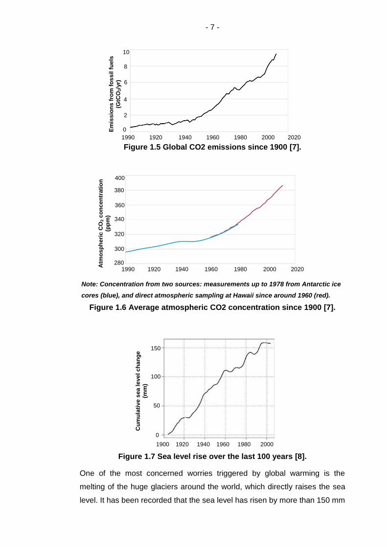
the outer space – like a thick quilt. Figure 1.5 shows a record of CO2

emissions since 1900 and it is clear that due to human activities, the global

CO2 emissions have increased by more than 1000% since 1900.

Consequently, the average atmospheric CO2 concentration level has

increased by over 30% from about 296 ppm in 1900 to about 390 ppm in

2010 (see Figure 1.6).

- 7 -

Figure 1.5 Global CO2 emissions since 1900 [7].

Note: Concentration from two sources: measurements up to 1978 from Antarctic ice

cores (blue), and direct atmospheric sampling at Hawaii since around 1960 (red).

Figure 1.6 Average atmospheric CO2 concentration since 1900 [7].

Figure 1.7 Sea level rise over the last 100 years [8].

One of the most concerned worries triggered by global warming is the

melting of the huge glaciers around the world, which directly raises the sea

level. It has been recorded that the sea level has risen by more than 150 mm

Em

iss

ion

s f

rom

fo

ss

il f

ue

ls

(GtC

O2/y

r)

8

10

6

4

2

0

1990 1920 1940 1960 1980 2000 2020

1990 1920 1940 1960 1980 2000 2020

Atm

os

ph

eri

c C

O2 c

on

ce

ntr

ati

on

(pp

m)

400

380

360

340

320

300

280

0

100

150

1900 1920 1940 1960 1980 2000

50

Cu

mu

lati

ve

sea

le

ve

l c

ha

ng

e

(mm

)

- 8 -

over the last 100 years (see Figure 1.7). If we allow global warming to

continue to develop without any control, then in several centuries that most

of the land will be under the sea.

Facing this challenge, national and international efforts have been made to

reduce greenhouse gas emissions. The Kyoto Protocol international

agreement announced in 1997 that in order to commit countries who are

members of the United Nations Framework on Climate Change (UNFCC) to

reduce greenhouse gas emissions [9]. In Europe, short term and long term

targets have been made regarding to greenhouse gas emission reduction:

EU members have committed themselves to reducing greenhouse gas

emissions by 20%, while increasing the share of renewables in the energy

mix to 20% by 2020 [10]. In 2011, the EU confirmed a long term objective of

reducing greenhouse gas emissions by 80-95% by 2050 compared to 1990

[10].

The UK, under the framework of UNFCC and the EU, aims to reduce 34% of

the greenhouse gas emissions by 2020 and have a further reduction to 80%

by 2050 compared to the 1990 level. Other major countries, such as China,

United States, Canada, India and Brazil, have started their own program and

policies to reduce greenhouse gas emissions [11].

1.3 Carbon capture technologies

The typical CO2 emission rate from a conventional coal-fired power plant can

be as high as about 906 kg/MWh [12]. Therefore, coal-fired power plants are

regarded as one of the most significant boosters to the atmospheric CO2

level. For example, from the top 50 dirtiest power plants in the USA, only

less than 1% of the total number, produced 50% of all the USA’s vehicle

carbon emissions [13]. Considering the importance of coal (see Section 1.1),

coal still occupies a large share of the energy mix and will do so in the

foreseeable future. Current environmental situations and government

policies push energy extensive industries, especially coal-fired power plants,

to develop new low carbon technologies.

Carbon Capture and Storage (CCS) represents a set of technologies that

can capture more than 90% of the CO2 produced from burning fossil fuels in

- 9 -

electricity generation and other industrial processes, thus preventing the CO2

from being emitted to the atmosphere. The captured CO2 is liquefied and

then transported by either pipe lines or ships to a suitable underground

storage site which can be saline aquifers or depleted oilfields. Moreover, the

stored CO2 can be utilised in other industrial sectors where pure CO2 is required.

It has been acknowledged that the utilisation of CCS is a necessary way that

people can keep fossil fuels in the world’s electricity supply mix while still

meeting the greenhouse gas reduction requirements [14].

Generally, CCS technologies can be classified into three categories using

different technique procedures, and these are pre-combustion, post-

combustion and oxy-fuel combustion and the following part of this section

provides a brief introduction to these three types of CCS technologies.

1.3.1 Pre-combustion

Figure 1.8 shows a simplified process diagram of the pre-combustion

process. In pre-combustion technique, the CO2 is captured before the

combustion process [15]. In the beginning, an air separation unit is used to

produce pure O2, which is then mixed with a suitable amount of coal/fuel in a

gasifier where a synthesis gas mainly consists of CO and H2 [15]. Further,

the synthesis gas is passed to a reactor where the shift reaction with water

takes place so that a mixture of CO2 and H2 is produced. Then, the CO2 can

be captured, compressed and sequestered while the H2 can then be

combusted in a gas turbine or a burner to generate thermal energy and more

importantly the flue gas (mainly H2O) from combustion is 100% clean.

Air Separation

Unit

Air

H2Gasifier

CoalShift Reactor

CO & H2CO2 Capture

CO2 & H2

CO2 Compression

CO2

CO2 for storage

Gas Turbine

N2

O2

Figure 1.8 A simplified diagram for the pre-combustion process [16].

In the electricity generation sector, the pre-combustion technology can be

used with carbon capture in an integrated gasification combined cycle (IGCC)

power plant. A significant advantage of the IGCC power plant with carbon

- 10 -

capture is that its efficiency is about 7 - 9% higher compared to those of the

oxy-fuel or post-combustion power plants [17]. However, the construction of

IGCC power plants requires a high capital investment and this technology

cannot be applied to the existing coal-fired power plants. Currently, pre-

combustion technology is not yet fully commercialized. In the UK, several

IGCC power plant projects are under consideration/construction, namely the

Teesside Low Carbon Project (450 MW) with a CO2 capture ratio of 85%, the

C.GEN North Killingholme Project (450 MW) in Yorkshire and the Don Valley

Power Project (650 MW) in Yorkshire [18]. However, up to now, these

projects have not been commissioned.

1.3.2 Post-combustion

Figure 1.9 represents a simplified process diagram of the post-combustion

process where the CO2 capture process takes place after the combustion in

the furnace [19]. The capture of CO2 could be achieved by allowing the flue

gas to pass through some chemical solvent, which can be

monoethanolamine (MEA) or methylenedioxyethylamphetamine (MDEA) or

mixtures of them [19]. Then the CO2-rich solvent is heated to release the

captured CO2 which is almost pure and ready for compression, and

meanwhile the CO2-lean solvent is regenerated and recycled to the CO2

capture loop. In addition, just before the CO2 capture process, a gas

cleaning process, where a flue gas desulphurisation (FGD) unit is employed,

it is necessary to remove the SO2, which has an oxidative degradation effect

on the MEA/MDEA solvent [20].

FurnaceAir & Coal CO2 & N2

Gas Cleaning CO2 Capture

CO2

CO2 Compression

CO2 for Storage

Pollutants Treated Gas

Figure 1.9 A simplified block diagram for the post-combustion process [16].

- 11 -

Post-combustion technology is a promising candidate for carbon capture and

storage because it can be directly used to retrofit the existing coal-fired

power plants. However, the integration of this technology would result in an

efficiency penalty ( about 10% of the efficiency penalty with 90% of the CO2

captured [21] ) to the power plant because the regeneration of the lean

solvent requires a steam extraction from the steam turbine to provide the

necessary heat for the chemical reactions.

The world’s first commercial-scale post-combustion CCS project

(SaskPower Integrated Carbon Capture and Storage Demonstration Project

[22]) has been in operation in Canada. At full capacity, the post-combustion

facility captures over 1 million metric tons of CO2 per year, reflecting a 90%

CO2 capture ratio from a 139 MW coal-fired unit [22]. In July 2014, the

world’s largest commercial post-combustion project (Petra Nova Project [23])

was announced in the USA. This project aims to install the post-combustion

technology to the coal-fired W.A. Parish Generating Station to annually

capture 1.4 million metric tons of CO2 from a 240 MW coal-fired facility, with

a 90% CO2 capture ratio [23]. In the UK, a commercial post-combustion

project, based on the Peterhead gas-fired power station in Aberdeenshire is

under consideration [24] and the planning application is expected to be

submitted in 2015.

1.3.3 Oxy-fuel combustion

Oxy-fuel combustion technology offers a viable low carbon pathway for the

existing coal-fired power plants to enable CO2 capture and storage. The

conventional coal-fired furnaces use air as the oxidant in the combustion

process where the CO2 concentration in the flue gas is diluted by the

nitrogen. In contrast, as is shown in Figure 1.10, the oxy-coal combustion in

a furnace takes a mixture of oxygen and recycled flue gas as the oxidant gas

in order to significantly increase the concentration of CO2 in the flue gases

[25]. Generally, the purity (vol%) of the O2 used in the oxy-coal combustion

is not less than 95% and for this purpose an ASU is employed [25]. The

recycled flue gas is for the purpose of the flame temperature control and

makes up the volume of the separated N2 to ensure there is sufficient gas to

transfer the combusted heat to the heat exchangers. After the oxy-coal

combustion, a flue gas, mainly consisting of H2O and CO2, is produced,

- 12 -

which is ready for compression and storage after a gas cleaning process

where the SOx is removed [25].

Air Separation

Unit

Air

N2

Furnace

Coal

O2Gas Cleaning

CO2 Compression

Flue Gas Recycle CO2 for Storage

Figure 1.10 A simplified block diagram for the oxy-fuel combustion process [16].

It should be noted that the use of an ASU in this technology brings in an

energy penalty of about 10% [26] to the power generation system. The

preferred method for the ASU is cryogenic distillation, since this technology

currently is commercialised and is capable of producing a large amount of

high purity oxygen compared to other oxygen separation technologies [27].

At the moment, oxy-fuel technology has not been commercialised and the

Callide Oxy-fuel Project [28] is the only demonstration project of a oxy-fuel

power plant in the world. The air-coal Callide-A power station in Queensland

having a full load of 30 MW is retrofitted to an oxy-coal power plant.

In the UK, a oxy-fuel demonstration project with a gross output of 448 MW,

named the White Rose CCS project [29], has been announced and the oxy-

fuel power plant will be situated near to the Drax Power Station.

1.4 Power generation system modelling

System computer modelling techniques enable engineers to research and

evaluate the power plant operation, optimisation and control policies so that

the potential risk and cost of operating/constructing the power plant can be

reduced.

In the modelling of a coal-fired power plant, accurate modelling of the boiler

is important because even a small change in the combustion environment of

the boiler may pose a significant impact on the overall performance of the

- 13 -

plant. In the boiler, the complex coal combustion process takes place and

energy is released from the coal. The combustion process involves several

steps: (i) the coal particle is preliminarily heated when entering the boiler; (ii)

the moisture content in the coal is evaporated; (iii) as the coal particle

absorbs more heat, the devolatilisation process takes place so that the

volatile matters and tar is released; (iv) the char content left in the particle

combusts as it is further heated. Correspondingly, in order to accurately

model the combustion process in the boiler, the devolatilisation, volatile

combustion and char combustion processes must be properly modelled. In

addition, the strong turbulence in the boiler as the turbulence has an effect

on the combustion process. Fortunately, computational fluid dynamics (CFD)

is an important modelling technology in researching the combustion and fluid

flow characteristics in the boiler and typically a commercial CFD code,

named ANSYS FLUENT, can be used to cover these problems. ANSYS

FLUENT employs the finite volume method to discretize the fluid domain

enclosed by the boiler into a huge number of cells based on which the

transport equations for the mass, momentum and energy balances are

solved. The continuum gas phase is solved in an Eulerian frame [30] while

the motion of the discrete coal particles is predicted in the form of a

Larganian frame [30].

Apart from the boiler, a coal-fired power generation system contains many

other components, such as the steam drum, steam turbines and the

condenser. In addition, the air separation unit and the amine capture plant

are involved in the whole system if carbon capture technologies are applied.

It is impossible to wholly depend on CFD techniques to model all of these

components due to the expensive computational resources and time

required. Fortunately, process simulation techniques can cover this gap and

there are several commercial process simulators available for this purpose,

such as ASPEN Plus, gPROMS, PRO/II, DYNSIM, etc. Generally, process

simulation employs simple mass and energy balance equations (zero or

one-dimensional) to describe the modelled unit and numerous empirical

parameters are employed. Therefore, the computational effort required is

quite small compared to that employed in the CFD modelling.

- 14 -

In order to take advantages of both the CFD and process modelling

techniques, integrated CFD and process co-simulation methods are

becoming state-of-the-art in the research on the performance and integration

of the power plant. It is clear that a 3D boiler CFD simulation usually takes a

long time to obtain converged results while the process simulation accounts

for the other components is much faster. Then if CFD and process modelling

techniques are directly linked in such a way that the CFD simulation has to

be performed at each of the operational conditions that are required in the

plant process model. This approach is straightforward but requires an

unacceptable amount of time for the CFD calculations to cover a whole

range of operational conditions of a power plant [31]. Therefore, the efficient

integration of CFD and process simulation techniques needs to be

considered. Hence the reduced order model (ROM) technology provides a

possible solution which is able to take the place of CFD models to very

quickly obtain the necessary information (such as the heat flux to the water

wall) to drive the process simulation [31].

1.5 Research aims, novelties and scope of the thesis

1.5.1 Research aims and novelties

Carbon Capture has been recognised as playing an important role in

reducing the CO2 emissions from coal-fired power plants so that coal can be

continued to be used in the energy mix. Both CFD modelling and process

modelling techniques have been confirmed as important methods for

investigating the application of the Carbon Capture technologies in the coal-

fired power plants. Therefore, this research aims to develop a CFD and

process co-simulation technique that can be depended upon to efficiently

evaluate the operations of the power plants using carbon capture techniques.

The novelties of this research are as follows:

i) More accurate reduced order models (ROM) have been developed to link

the CFD to the whole plant process model.

ii) A new approach has been suggested for estimating the potential of

retrofitting an existing power plant to oxy-firing.

- 15 -

iii) A feasible range of oxygen enrichments for the retrofitted power plant has

been identified at different power loads.

1.5.1 Scope of the thesis

Concerning the technical issues discussed in Section 1.4, the research to be

performed in this thesis can be divided into several milestones:

(i) In Chapter 2, a detailed literature review on oxy-coal system modelling

techniques is presented, which involves CFD modelling and process

simulation techniques. In the following Chapter 3, the experimental facility

and data that are required for the model set up and validation in the thesis

are summarised.

(ii) In Chapter 4, a set of combined CFD and process simulations is

performed on an experimental facility, which involves a 250 kWth coal

combustion furnace and a MEA based CO2 capture plant. The CFD

techniques are employed to solve the turbulence, chemical reactions, and

heat transfer in the coal combustion furnace while the process modelling

techniques are used to account for the modelling of the CO2 capture plant.

Then the reduced order models based on the CFD simulation results of the

furnace are linked to the process model for CO2 capture plant.

(iii) In Chapter 5, the research objective is extended to the modelling of a

large-scale coal firing power plant. A three dimensional CFD model for the

utility boiler of this power plant and a process model for the whole power

plant are developed. These efforts are the necessary preparations for

developing a CFD and process co-simulation approach that can be

employed to predict the operations of a power plant under both air-coal and

oxy-coal firing conditions.

(iv) Based on the CFD and process models developed in Chapter 5, a new

approach has been developed in Chapter 6 in order to estimating the

potential of retrofitting an existing power plant to oxy-firing. The three

dimensional CFD boiler model developed in Chapter 5 has been employed

to simulate the complex coal combustion and heat transfer to the boiler heat

exchangers under air-firing and oxy-firing conditions. Then, a set of reduced

order models has been developed to link the CFD predictions to the whole

plant process model, developed in Chapter 5, in order to simulate the

- 16 -

performance of the power plant under different load and oxygen enrichment

conditions if retrofitted to oxy-firing. The reduced order models are

generated based on the CFD simulations of the boiler using a non-linear

Kriging interpolation method. With this new CFD-process co-simulation

approach, the potential of retrofitting the Didcot-A power plant to oxy-coal

firing is analysed.

- 17 -

Chapter 2. Literature Review

This chapter provides a detailed literature review on the modelling

technologies with regard to the CO2 capture technologies that can be applied

to the existing or new built coal firing power plants. The combustion process

of the coal particles and modelling techniques are discussed in Section 2.1.

The considerations of heat transfer and turbulence in CFD modelling are

reviewed in Section 2.2. The process modelling approaches for the CO2

capture techniques that can be used in coal-fired power plants are discussed

in Section 2.3. Finally, a brief summary about this chapter is provided in

Section 2.4.

2.1 Coal combustion process modelling

Appropriate description and modelling of the combustion process of a single

coal particle is important as it is fundamental for the modelling of the coal

combustion in large scale boilers. The combustion process of a coal particle

undergoes four major stages as described in Figure 2.1. In the evaporation

process, the moisture content in the coal particle is evaporated; as the coal

particle is further heated, the devolatilisation process takes place, where the

volatile contents (light gases and tars) start to be released and react with the

oxygen, which is known as volatile combustion. Then, as the temperature of

the coal particle further increases, the char combustion process occurs,

where the remaining char is oxidised at a lower rate compared to the

devolatilisation and volatile combustion.

Evaporation Devolatilisation Volatile combustion Char combustion

Figure 2.1 Schematic of the combustion process of a coal particle

[32].

- 18 -

It should be noted that the above description on the combustion process of a

coal particle assumes that each stage takes place in a sequential order and

this assumption is adopted in the current CFD codes. However, in fact, some

of the stages may overlap.

2.1.1 Evaporation and devolatilisation

As the coal particle is heated by the surrounding gas quickly, the water

evaporates fiercely once the temperature reaches the boiling point and the

water escapes from the surface of the particle through many pores in the

particle. During the evaporation process, the particle may shrink or break

into smaller pieces, but this effect is currently not considered in the

modelling techniques.

When the temperature increases further to about 600 K [33, 34], the light

gases and tars, namely the volatile contents, begin to leave the particle

through pores to the external gas phase and their subsequent oxidisation

generates mainly CO2 and H2O. The physical structure of the coal particle

changes significantly, which is related to the release of the volatile matter,

and a swelling phenomenon can be observed [35]. The devolatilisation

process is fundamentally affected by the coal type, temperature, pressure

and the species of the surrounding gas [34]. After the devolatilisation

process, the solid material remaining in the particle is the char, which has a

porous structure. In fact, the structure and reactivity of the char is affected by

the devolatilisation process [32, 36].

Clearly, the amount of volatile content released from devolatilisation varies

for different coal types. Coal can be classified into three main categories,

namely the lignite, bituminous and anthracite, according to their ages [32].

As the youngest coal, lignite is comparatively soft and mainly contains

moisture and volatile matters with low fixed carbon, while the anthracite, as

the oldest coal, is comparatively hard and mainly contains fixed carbon with

little moisture and volatile matter [32]. The amount of volatile matter present

in the bituminous coal lies between the other two types of coal [32]. In

addition, it had been found that the amount of volatile matter released could

be enhanced by a higher peak temperature and higher heating rates [37-39].

The amount of the volatile matter in the coal can be measured from a drop-

- 19 -

tube furnace with controls on the heating rate. A factor called the ‘high

temperature volatiles yield ratio’ is usually employed to describe this

enhancement by comparing the amount of the obtained volatiles to that

measured from a standard proximate analysis [37].

The rate of devolatilisation can be modelled by a single-rate model [39]

using a single Arrhenius formation where the devolatilisation rate is assumed

to be proportional to the volatiles remaining in the particle. As a matter of

fact, the volatile mater leaves the particle at various rates, thus the single-

rate model may be insufficient to accurately describe the process. A more

suitable solution with higher fidelity would be the two-competing rate model,

which was developed by Kobayashi et al. [40]. The two-competing rate model

relies on six parameters and is capable of modelling most coals, if the

corresponding data for the coal is available. Silaen et al. [41] investigated

different devolatilisation models as a part of a CFD code. They found that

the two-competing rate model predicted a slower devolatilization rate than

the single-rate model but produced a higher exit gas temperature and higher

CO2 mass fractions. However, experiments were not performed. The Sandia

National Laboratories [42] performed a number of experiments and found

that the model constants used by Kobayashi et al. [40] could not give

satisfying predictions on some coals, while the constants used by

Ubhayakar et al. [43] appeared to increase the accuracy.

Network models, such as the chemical percolation devolatilisation (CPD)

model [44], the functional group-depolymerisation vaporization cross-linking

(FG-DVC) model [45] and FLASHCHAIN [46], can predict the devolatilisation

rate and the yields of gases and tars under different heating rates if the

structure parameters of the coal particle are available. Jones et al. [47]

evaluated different devolatilisation models and concluded that the network

models could provide satisfactory devolatilisation rates. William et al. [48]

performed experiments on a drop-tube furnace for a range of coals and the

experimental results were compared to the predictions from the CPD, FG-

DVC and FLASHCHAIN models and the predictions on the volatile yields

were in generally good agreement with the experimental data, although

these models predicted slightly different results.

- 20 -

Rastko et al. [49] implemented the single rate, two competing rates, CPD

and FG-DVC model as a part of a CFD code in order to numerically

determine the ignition point of a bituminous coal in a laboratory ignition test

facility under air and oxygen enriched environments. The predictions

suggested that the network models (CPD and FG-DVC) provide more

accurate results compared to the single rate and the two competing rates

models and the best performance was achieved by the FG-DVC model.

However, the authors indicated that the use of the FG-DVC model would

require much more computational resources, since the additional transport

equations for the volatile species need to be solved. The results also

revealed that the devolatilisation models, which were originally developed for

conventional air combustion, can be applied to oxygen enriched combustion

conditions. Moreover, Shaddix et al. [50] found that the switching to an

oxygen enriched combustion environment has little impact on the

devolatilisation process if the combustion temperatures are kept the same.

2.1.2 Volatile combustion

The volatile matters are released from coal particles mainly contain CO, CO2,

H2O and many hydrocarbons [36]. The volatiles then react with the

surrounding oxidiser gas to produce CO2 and H2O with numerous

intermediate products. Therefore, the accurate description of the volatile

combustion process involves a large number of intermediate reactions and

species [32], which would pose a significant challenge for the CFD modelling

as numerous chemical mechanisms and transport equations need to be

solved. A popular solution and simplification is a global mechanism, which

assumes the reaction rates to be very fast and greatly reduces the number

of reactions and species. The global mechanism assumes the volatile

matters to be a single material CxHyOz and its oxidisation can be

represented as the following two step reaction [51]:

x y z 2 2

y 2x+y-2zC H O +αO xCO H O, where α

2 4 (2.1)

2 2

1CO O CO

2 (2.2)

In this global mechanism, an intermediate species ‘CO’ is introduced to

describe the char oxidation occurring on the particle surface and the

http://www.sciencedirect.com/science/article/pii/S0016236111000949

- 21 -

intermediate CO is further oxidised to CO2. In fact, the complex combustion

process is highly determined by the turbulent mixing, which affects the

kinetic rates of the reactions.

For the laminar flames, the reactions in the combustion gas phase can be

described by the kinetic rates. However, in a pulverized coal combustion

furnace, the volatile combustion is significantly coupled with the strong

turbulence. It is known that strong turbulence may greatly enhance the

reaction rates [52] and this makes the global mechanism theoretically

applicable. In fact, the proper selection of an approach to model the volatile

combustion involves several aspects that need to be considered: accuracy,

the ability to describe the chemical reactions and the computational

requirement.

The eddy dissipation model (EDM) [53] relates the reaction rates with the

turbulence level. However, this model ignores the chemical kinetics, thus it

does not account for the intermediate species and can be only used with the

global mechanism. The EDM has been widely used for modelling the

pulverized coal combustion process [54-57]. The eddy dissipation concept

model (EDCM) [58], as an expansion of the EDM, takes the detailed

chemical kinetics into consideration and therefore this model can describe

the intermediate reactions and products. However, this requires the solution

of the transport equations for each species, and thus the demand on the

computational resources is significantly higher.

The laminar flamelet model [59] treats the turbulent flame as a set of laminar

flamelet regions. This model considers a larger number of chemical

reactions and intermediate species. The characteristic of this model is that

the density, species fractions and the temperature profile near the flamelet

are described by the mixture fraction and the scalar dissipation rate [60].

However, the scalar dissipation rate needs to be modelled separately.

Combined with a PDF, the flamelet model can be used to model the

turbulent flames.

The application of the probability density functions (PDF) [61] provides a

promising option to address the chemical kinetics in the combustion flows.

The significance of this approach is that the chemical source term can be

- 22 -

easily expressed. However, this approach is computationally expensive. The

mathematic formation of the PDF needs to be assumed, such as the -PDF .

William et al. [48] compared the PDF model to the finite rate model in the

CFD calculations and found that the predictions from the PDF model showed

a better agreement with the experimental data.

2.1.3 Char combustion

Once the volatile matters have been released from the coal particle, the

remaining material is the char content, which mainly includes free carbon

and incombustible matters. The combustion process of the char involves a

number of issues that need to be considered, such as the temperature, coal

type, particle size, surface area, oxygen fraction in the surrounding gas and

the resident time in the high temperature flame region [32]. Although a large

amount of research has been devoted, both numerically and experimentally,

the char combustion mechanism is not yet fully identified due to the complex

pore development and mass transfer in the char combustion process [62].

The char combustion is mainly dominated by the reaction between the

carbon and the oxygen, which produces CO and further CO2. The fractions

of CO and CO2 are fundamentally determined by the local temperature. A

higher CO fraction is usually found at high temperature locations (such as

the particle surface), where the CO2 fraction is quite low [32]. In addition, the

gasification of the carbon by CO2 and H2O may occur at high temperatures,

therefore the char reactions can be described by the following equations:

2

1C O CO

2 (2.3)

2C CO 2CO (2.4)

2 2C+H O CO+H (2.5)

It should be noted that when the oxygen concentration is comparable to the

CO2 concentration, the gasification reactions become less important [63],

especially in the pulverized coal fired boiler of a power plant. Therefore, the

gasification reactions were ignored in these CFD investigations [56, 57, 64]

on the pulverized coal combustion process in coal fired boilers and this

results in a satisfactory agreement with the experimental data being

obtained.

- 23 -

The diffusion limited model, which was developed by Baum and Street [33],

calculates the reaction rate based on the oxygen diffusion rate to the char

surface, but this model ignores the impact of the chemical kinetics. As an

improvement, the kinetics-diffusion limited model [33] takes both the oxygen

diffusion rate and the chemical kinetics into consideration. Simulation results

using the kinetics-diffusion limited model were performed in [65] and the

predictions on the temperature showed a good agreement with experimental

data. However, it should be noted that these methods do not consider the

exact char shape or the particle swelling.

Clearly, the char porosity enhances the reaction area of the char particle,

which has a fundamental impact on the char oxidisation. Therefore, in order

to account for the effects introduced by this factor, the intrinsic model [66]

was proposed, which considers the char porosity and the change in the

surface area throughout the combustion process. Specially, this model

regards the reaction rate as a combination of the pore surface diffusion and

the intrinsic reactivity [67]. The simulation results obtained from the intrinsic

model and the kinetics-diffusion limited model were separately compared to

the experimental data in [48] and found that the intrinsic model predicted

more accurate results.

The carbon burnout kinetics (CBK) model [68] was developed based on the

intrinsic model and this model considers more effects, such as thermal

annealing, statistical kinetics, statistical densities, and ash inhibition in the

late stages of the char combustion [68]. Gharebaghi et al. [69] employed the

CBK model to investigate the char combustion kinetics under oxy-coal

combustion conditions and modifications have been made on the CBK

model in order to make it applicable to oxygen-enriched environments. It

was found that the modified CBK model improved the accuracy of the

burnout prediction under both air-coal and oxy-coal conditions.

In a CO2/O2 environment, Kuhr et al. [70] numerically found that the

consideration of the C-CO2 reaction improved the oxygen predictions

compared to the experimental data. This investigation reveals that in the

CFD simulations for oxy-coal combustion systems, the consideration of the

gasification effects may be important. However, oxygen concentration is

- 24 -

usually higher near the burner region, where the gasification reactions are

less important, while the oxygen concentration near the boiler exit is usually

much lower (0-5%) and gasification effects become important, but in the exit

region, most of the particles have been burnt out.

2.1.4 Pollutant formation

Coals contain small fractions of sulphur and nitrogen and the fractions vary

with different coal types. The sulphur and nitrogen content can produce

pollutants, such as SOx and NOx, during coal combustion. These pollutants

are harmful to the environment, thus it is necessary to model the

mechanisms for the SOx and NOx formation during coal combustion.

However, the detailed pollutant formation mechanisms can be safely ignored

if the CFD simulation is focused on the overall heat transfer characteristics

[56, 57], since the quantities of the pollutant gases are quite small compared

to other species. During the coal combustion process, NOx is mainly

generated through three different manners: thermal NOx, prompt NOx and

fuel NOx and NO is considered as the most significant form of NOx, since it

accounts for about 90% of the total NOx produced.

2.1.4.1 NOx formation

In the thermal NOx mechanism, NO is formed from the reaction between O2

and N2 at high temperatures, which can be described by the Zeldovich

mechanism:

2O N NO+N (2.6)

2N O NO+O (2.7)

A combination expression of the above two reactions can be written as:

2 2O N 2NO (2.8)

where overall reaction rate is highly temperature dependent and its

mathematical expression can be found in [32]. Since the overall reaction is

slow, equilibrium concentrations of NO are built up only in situations where

the residence time is sufficient, i.e. in large boilers. In smaller boilers, the

thermal NO formation is limited by the lower residence time.

The prompt NO mechanism was found by Fenimore [71] and it accounts for

the formation of NO from reactions involving N2 and carbon-containing free

- 25 -

radicals, which can be the intermediate species from the volatile combustion.

The formation of prompt NO involves a number of reactions which have

been summarised in [32]. Prompt NO mainly occurs in fuel-rich flames with

short residence times and only accounts for a small part of the total NO.

The fuel NO mechanism is the dominant form of NO production throughout

the coal combustion process. The fuel-N contained in the coal is separated

into two groups after the devolatilisation process: one group is named

volatile-N and the other one is called char-N [72]. The volatile-N is mainly

HCN and little NH3 [32]. Then the volatile-N is oxidised to produce NO or N2

and their relative amounts depend on the concentration of the fuel-N in the

fuel; if rich, all HCN would produce N2 [32]. The char-N mainly forms NO and

more than 75% of N is converted to NO in high temperature regions. The

difficulty for modelling the fuel NO is the accurate prediction of the ratios of

the char-N and volatile-N and the ratios can be directly obtained by

experiments or by the devolatilisation models described in Section 2.1.

Álvarez et al. [73] integrated different network models with CFD techniques

to predict the volatile-N and char-N formation from several types of coals

under both air-coal and oxy-coal conditions. The HCN to NH3 ratio from the

volatile-N can be directly obtained by the network models; as for the char-N,

the HCN to NH3 ratio was approximated by a conversion coefficient. The

network model FG-DVC was found to produce accurate predictions for all

the investigated coals. Álvarez et al. [74] also investigated the NO formation

using FG-DVC model and found that FG-DVC could give reasonable

predictions at different temperatures and heating rates, but also found that

the results for the air-coal and oxy-coal conditions showed little difference.

Several approaches are available to reduce the NO production during, such

as, the low-NOx burner, the SCR (selective catalytic reduction) and the

reburning technique.

2.1.4.2 SOx formation

Coal also contains sulphur and the sulphur content can be oxidised to

produce SO2 or SO3, which are known as acid gases and may corrode the

process devices with the presence of moisture. The release of sulphur is

similar to the release of fuel-N during devolatilisation, and therefore the



- 26 -

sulphur can be similarly regarded as volatile-S and char-S. It was found that

the formation of SO2 in oxy-coal combustion is significantly higher than that

in air-coal conditions [75]. However, the SO3 formation is lower than that

under air-coal conditions.

2.1.4.3 Soot formation

Soot is a mixture of impure carbon particles due to the incomplete

combustion of the hydrocarbons. Soot is a pollutant, which is believed to

disturb the radiative performance of the combustion gas, and a previous

investigation [76] indicated that the neglecting of the soot in the coal

combustion modelling would cause large errors in the temperature

predictions. However, the soot formation mechanism is not yet fully

understood and further modelling and experimental work is required [77].

A widely used model for modelling the soot formation was proposed by

Brown et al. [76]. However, this model depends on some empirical

parameters, which were obtained from air-coal combustion experiments,

thus it could be only applied to air-coal combustion modelling with

confidence. It has been found that the soot formation depends upon the

stoichiometry in the combustion regions [78], thus this ignored the

differences between the air-coal and oxy-coal conditions. However, a further

investigation [79] found that the soot formation in the oxy-coal environments

is lower than that in air-coal environments.

2.2 Heat transfer and turbulence

Computational fluid dynamics (CFD) techniques provide a viable tool for

investigating the coal combustion process, since CFD techniques

incorporate the complex geometries of the coal fired boilers and detailed

numerical models on heat transfer and turbulence. The finite volume method

(FVM) is widely used by most CFD codes to discrete the governing

conservation equations over the computational regions characterised by a

number of computational cells. The use of non-uniform grids can ease the

difficulty in meshing the burners or other complex geometries. The proper

meshing of the geometries is important as its quality may affect the accuracy

of the solutions, even if the sub-models for the particle combustion, heat

- 27 -

transfer and turbulence are properly set. Therefore, a large number of

meshing tutorials can be accessed online.

In fact, in order to accurately perform CFD simulations on the coal

combustion process in a coal fired boiler, it does not only include the

detailed models accounting for the coal particle oxidisation (Section 0), but

also involves proper sub-models incorporating heat transfer and turbulence.

2.2.1 Heat transfer

During the coal combustion process in a boiler, heat is released and then

transferred to the water/steam inside the water wall tubes surrounding the

furnace and the hanging tube heat exchangers. Heat transfer includes three

approaches: convection, conduction and radiation, and radiation is the

dominant form of heat transfer in the furnace region. However, in the region

far away from the furnace section, the gas temperature has been

significantly reduced, thus convection becomes dominant.

Radiation is quite extensive in the furnace, since it is proportional to the

fourth power of the temperature. Radiation is governed by the following

radiation transfer equation (RTE) [80]:

4

4,2

,0

(r,s)( ) (r,s) (r,s ) (s,s )

4

s

s

dI Ta n a I I d

ds

(2.9)

where is the wavelength, r is the position vector, s is the direction vector,

s is the scattering direction vector, s is the path length, a is the absorption

coefficient, n is the refractive index, ,s is the scattering coefficient, is

the Stefan-Boltzmann constant (8 2 45.669 10 /W m K ), I is the radiation

intensity, T is the local temperature, is the phase function and is the

solid angle.

The radiation intensity I is determined by the wavelength , spatial

position r , direction s and the solid angle . In order to accurately predict

the radiation, these techniques need to be wisely selected: a proper

approach to solve the RTE as well as the model to account for the

absorption and scattering properties of the gas and particles.

- 28 -

There are several approaches available to solve the RTE, namely the P-N

method [81], the discrete ordinates method (DOM) [82], the discrete transfer

method (DTM) [83], and the Monte Carlo method [84]. Both the P-N and the

discrete ordinates methods are applicable to the combustion flows since

these methods are able to conveniently incorporate the scattering,

absorption, and the emission effects of the combustion gas and particles.

The discrete transfer method is a ray-tracking approach which directly tracks

the paths of rays until the rays reach other surfaces. However, this method

neglects the scattering effects brought by the particles, which need to be

considered for the coal combustion environments as the interactions

between the particle-radiation are extensive. The Monte Carlo method is

also a ray-tracking approach and it employs statistical techniques to

calculate the radiation intensity that travels through the medium. This

method is considered to be accurate as it completely randomizes the

directions of the rays, however, the demand on the computational power

significantly increases.

In the boiler, the heat is released from the combustion of the coal particles,

which have strong interactions to the radiation field as they can either emit or

absorb the radiations. A simple solution that accounts for the effects of the

particles is to apply a gray assumption, which ignores the impacts introduced

by the different wavelengths. In this assumption, the particle-radiation

interactions are determined by the particle temperatures, size of the particles

and special distributions. A previous study [85] compared the particle-

radiation and the gas-radiation interactions under both air-coal and oxy-coal

conditions and found that the particle-radiation interactions are much more

extensive than the gas-radiation interactions.

In addition, the combustion gas contain some species with strong absorption

capacities, such as CO2 and H2O, and it should be noted that the CO2

concentration in the oxy-coal combustion is much higher compared to that in

the air-coal combustion. Therefore, the radiative properties of the

combustion gas needs to be addressed in the radiation modelling.

A number of approaches can be used to account for the radiative properties

of the gas phase and these approaches can be classified as the following

- 29 -

groups: line-by-line (LBL) models, band models and the global models [16].

Although the line-by-line models are considered to be accurate, the huge

demand on the computational power by the line-by-line models limit their

applications to the CFD investigations [86]. The band models can be

classified into narrow band and wide band models according to how they

treat the full spectrum. The narrow band models [87] directly split the full

spectrum into a set of intervals, while the wide band models [88] only

consider the important intervals whose wavelengths are more interacted with

the radiation field. Thus the wide band models are more computationally

efficient but it should be noted that these band models can be only solved

with ray-tracking approaches.

As a widely used global model, the WSGG model [89] employs a set of

polynomials, as functions of the temperature, to calculate the absorption

coefficients of the gas phase and the most widely used model parameters

were proposed by Simth et al. [90]. However, these parameters need to be

modified for the oxy-coal simulations as the original values could only be

applied in the combustion simulations where the CO2 concentration is much

lower than that in oxy-coal conditions [91]. Therefore, appropriate WSGG

parameters for oxy-coal combustion need to be obtained and a

straightforward approach is to fit the WSGG polynomials from the predictions

by the more fundamental models, such as the statistical narrow band (SNB)

model [92] or the line-by-line model [93, 94].

Based on the SNB model, Johansson et al. [91, 92] proposed new WSGG

parameters that are applicable in the oxy-coal simulations with different

concentration ratios of CO2/H2O and found that the new WSGG correlations

improved the accuracy of the radiation predictions. Compared to the band

models, the computation time was greatly reduced. Further, other new

WSGG parameters for oxy-coal combustion were developed by

Kangwanpongpan et al. [94]. The new WSGG parameters were fitted from

the results obtained by the LBL model and the accuracy of the radiation

predictions was improved.

The full-spectrum correlated-k (FSCK) model [86] is also a global model that

has been used in oxy-coal simulations. Porter et al. [95] employed the non-

- 30 -

gray FSCK model and the gray WSGG model to calculate the radiative

properties under both air-coal and oxy-coal cases. It was found that the

non-gray FSCK method provided predictions with better agreement with the

benchmark data for all of the cases, while the gray WSGG model tended to

give over-predicrions. However, the computation time required by the FSCK

model is much higher than the gray WSGG model.

2.2.2 Turbulence

Strong turbulence can be observed in coal-fired boilers and turbulence is an

important factor that needs to be properly considered as it affects every

aspect of the coal combustion process, including mass transfer, chemical

reactions and heat transfer. Turbulent models in CFD can be classified into

three groups, namely direct numeric simulation (DNS), large eddy simulation

(LES) and the Reynolds-averaged Navier-Stokes (RANS) method, according

to their ability to model the details of the turbulence [80].

2.2.2.1 Direct numerical simulation (DNS)

The DNS approach dynamically solves the entire range of turbulent scales,

which is quite computationally expensive [80]. Thus this method is currently

not suitable to be applied to modelling the coal combustion process in

boilers, where strong turbulence and complex chemical reactions take place.

It should be noted that DNS is accurate, and therefore it can provide

validation data for the LES and RANS when the experimental data is not

available [96].

2.2.2.2 Reynolds-averaged Navier-Stokes (RANS) method

The RANS method is widely employed in the industry as it is much less

expensive in terms of computational demand, and more importantly it can

give satisfactory predictions if the model is properly set. RANS takes a

statistical view on the flow field and completely averages the control

equations. From the view of RANS, the field variables, such as the velocity

u , contain a mean component (u ) and a fluctuating component (u ). The

fluctuating component is assumed to have a mean value of 0 ( 0u ).

Therefore, u can be decomposed as:

u u u (2.10)

- 31 -

Applying the RANS decomposition to the momentum equation, the averaged

momentum equation, namely the RANS equation, can be written as:

( )( ) 2

( ) ( )3

i j ji l ii j ij

i i j i l j i

u u uu u upu u

t x x x x x x x

(2.11)

In the above equation, the additional term “Reynolds stress” is the product

from the RANS decomposition that needs to be modelled by the turbulent

models, which includes the eddy-viscosity models and the Reynolds stress

models.

The eddy-viscosity models are based on the Boussinesq hypothesis [97],

which assumes the Reynolds stress is proportional to the mean strain rate

and the Reynolds stress is modelled as:

2

- ( ) ( )3

ji ki j t t ij

j i k

uu uu u k

x x x

(2.12)

where t is the turbulent eddy viscosity, k is the kinetic energy and ij is

the Kronecker delta. It should be noted that the turbulent eddy viscosity t

needs to be modelled and a number of models have been developed for this.

The Prandtl mixing length model [98] is a zero-equation model that assumes

that the turbulent viscosity is proportional to the square of the length scale.

The Spalart Allmaras model [99] is a one-equation model that solves a

viscosity variable in a transport equation, then the viscosity variable can be

used to calculate the turbulent viscosity. In addition, the two one-equation

models for modelling the turbulent viscosity include the k and the k

models, which employ two additional transportation equations for the

turbulent kinetic energy k and either the turbulent dissipation rate or the

specific dissipation rate ( = k ). The turbulent viscosity t is calculated

as a function of k and or . A main advantage of these models is their

comparatively low requirements on the computational resources.

The k models have a number of variants, such as the standard k

[100], RNG k [101] and the realisable k model [102]. The standard

Temporal

term

Convention

term

Pressure

difference

Reynolds

stress

Viscosity

- 32 -

k model assumes that the flow is completely turbulent and ignores the

effects of the molecular viscosity, thus this model can be only used for fully

turbulent conditions. In order to apply the standard k model to other

situations, modifications have been made, and hence the RNG k and the

realisable k models were proposed. The RNG k model is based

on the statistical renormalisation group approach and it introduces an

additional term for the equation so that the accuracy for the low-Reynolds

and strained flows is improved. The RNG k model has been used in the

pulverised coal combustion simulations [103, 104]. As another variant, the

realisable k model depends on a modified transport equation so that

the model satisfies certain mathematical constraints on the Reynolds stress,

which are not realised in the standard k or the RNG k models. It

should be pointed out that both the RNG and realizable k models are

able to give more accurate predictions of the flows involving strong vortices

and rotations, compared to the standard k model. The standard k

model [105] and the shear-stress transport (SST) k model [106] both

employ transport equations for k and . The standard k model is

suitable for the low-Reynolds number and shear flows. The SST k model

blends the accuracy and the robustness near the wall and employs an

additional derivative term in the transportation equation. Therefore, the

SST k model can be applied to a wider range of flows with adverse

pressure gradients and separating effects.

The Reynolds stress model (RSM) [107, 108], is a more advanced RANS

model as it does not require the isotropic assumption which is used in the

previously introduced turbulent models. In order to solve the Reynolds-

averaged Navier-Stokes equations, the RSM introduces additional transport

equations for the Reynolds stress as well as the dissipation rate. Therefore,

seven transport equations are involved in a three dimensional problem,

which results in the computational cost being increased.

2.2.2.3 Large eddy simulation (LES)

A turbulent flow contains numerous eddies with different temporal and

spatial scales. The RANS approaches apply a Reynolds-average on all the

eddies, and thus all instantaneous information of the eddies are ignored. In

- 33 -

the LES method, only the small eddies are modelled, while the larger eddies

are directly resolved. Therefore, the overall computational cost required by

LES lies between those of RANS and DNS.

Compared to DNS, much coarser grids and larger time steps are allowed in

LES, since only the large eddies are resolved. However, when compared to

RANS, LES requires a much finer grid and smaller time steps, and thus a

LES simulation requires much larger computational resources and longer

computation time in order to obtain converged predictions. The practical use

of LES in the industry needs to be implemented by the employment of high-

performance computers.

In order to distinguish the larger eddies from the small eddies, the LES

applies a filter [109] to the Navier-Stokes equations, and the filtered

momentum equation can be written as:

( )( ) 2( )

3

( )

i j ji l iij

i i i l j i

i j i j

j

u u uu u up

t x x x x x x

u u u ux

(2.13)

A new term ( i j i ju u u u ) on the right-hand side of the equation, namely the

sub-grid-scale (SGS) stresses, is generated from the filtering and needs to

be modelled for the small scale eddies. The SGS stresses contain a

deviatoric and a isotropic part, which can be treated as the filtered static

pressure [110]. A number of models have been developed to solve the SGS,

such as the Smagorinsky-Lilly model [111], the dynamic Smagorinsky model

[112, 113], and the wall-adapting local eddy-viscosity model [114].

Edge et al. [54] employed a LES approach in a CFD model to simulate the

firing of a pilot-scale pulverised coal furnace under both air-coal and oxy-

coal conditions. The predictions from the LES was compared to the

experimental data as well as the results predicted by a RANS approach

incorporating the standard k model. The comparison indicated that the

LES approach is able to give more accurate predictions on the recirculation

and flame properties than the RANS method .

- 34 -

Similarly, Gharebaghi et al. [55] employed LES and RANS to simulate a 1

MWth combustion test facility under both air-coal and oxy-coal environments.

The predictions from LES were compared to RANS and experimental data

and it was found that although LES was able to capture more realistic details

of the flame, the improvement on the temperature predictions was not

significant. The authors suggested that further fundamental investigations

and improvements on the physical sub-models are necessary. In this case,

Clements et al. [115] evaluated the LES and the RANS models in the

simulation of a pilot-scale 250 kWth furnace under both air-coal and oxy-coal

conditions. The investigation employed the grey WSGG model and the non-

grey FSCK model to calculate the radiative properties of the gas phase. It

should be noted that both the WSGG and the FSCK models were integrated

with RANS, while only the FSCK model was used with LES. The simulation

results indicated that the variation in the gaseous radiative property models

does not significantly change the temperature or heat transfer predictions for

the RANS cases, while the LES combining with the FSCK model was

observed to provide more accurate results compared to the RANS model.

However, the interaction between LES and the grey WSGG model was not

investigated, thus a conclusion on the efficiencies for different combinations

of the turbulent and radiation models could not be drawn.

Considering the complexity as well as the high computational demand of

LES, a RANS approach rather than the LES is used to model the turbulence

in the later part of this thesis. It should be pointed out that CFD simulation of

the coal combustion in a boiler is not the final target. This thesis integrates

the CFD techniques with process simulation approaches in the simulation of

the carbon capture technologies so that a number of three dimensional CFD

simulations need to be performed, and thus it is not necessary to depend on

LES.

2.3 Carbon capture process modelling

The post combustion and the oxy-coal combustion technologies are the

carbon capture technologies that can be applied to either the existing or the

new built coal (or biomass) fired power plants. System process simulation

plays an important role in the development of the industries because it


- 35 -

assists engineers to better understand the operations, responses and

performances of the whole system and it is able to predict the optimised

operating conditions of the system, and therefore a large amount of

expenditure on experiments can be saved. This section provides a brief

literature review on the process modelling techniques with regard to these

two technologies.

2.3.1 Chemical absorption process modelling

A well identified advantage of using the post combustion techniques is that

this type of technologies requires the least modification to the original

combustion system. Post combustion technology refers to a set of

approaches that capture the CO2 from the flue gas after the combustion

process and the major approaches are the chemical absorption, adoption

and membrane separation [116]. However, chemical absorption is the only

technology that has the potential to be applied in large-scale commercial

power plants.

2.3.1.1 General process treatment

In the chemical absorption process, CO2 in the gas phase is absorbed by a

chemical solvent via chemical reactions to generate an unstable

intermediate compound, which then can be post-processed to regenerate

the original chemical solvent and release a high-purity CO2 stream [117]. A

number of amine solvents can be used to absorb CO2 and these solvents

have different absorption capacities, chemical stability and different

corrosion factors [118]. Currently, MEA is the most popular solvent for

capturing CO2 from pulverised coal power plants [19], as it is able to treat the

flue gas containing low CO2 concentrations.

Before the absorption process, some trace gases in the flue gas, such as

SOx and NOx, need to be removed because they may react with the MEA to

form other salts, thus the MEA solvent may be degraded. The removal of

SOx can be achieved by allowing the flue gas pass to through a flue gas

desulphurisation (FGD) equipment, while the NOx can be removed by a

selective catalytic reduction (SCR) device. In addition, the ash particles in

the flue gas has to be separated out as the solid particles may accumulate

- 36 -

and block the pipe lines of the CO2 capture plant and the removal of the ash

content can be performed by an electrostatic precipitator (ESP).

In Figure 2.2, the flow diagram demonstrates a CO2 absorption process

using a MEA solvent. Flue gas entering the absorber has to be cooled down

to about 320 K, which is identified as a feasible temperature range that could

reduce the solvent loss from evaporation and provide a suitable initial

temperature for the absorption reactions [119]. In the absorber, the rising

flue gas contacts with the downward lean MEA solvent flow and CO2 is

absorbed, and therefore a rich solvent is produced at the bottom of the

absorber. The typical CO2 loading of the lean MEA solvent is between 0.1-

0.3 (mol CO2 per mol MEA), while a rich loading is usually between 0.4-0.5

[120]. During the CO2 absorption, heat is released from the chemical

reactions and the temperature of the lean solvent increases, which leads to

the evaporation of the water content, and thus the MEA solvent becomes

more concentrated. Therefore, in order to maintain the water balance in the

solvent, the treat flue gas undergoes a water wash process so that the

moisture can be condensed and recycled to the solvent.

Figure 2.2 A process flow diagram for CO2 capture using chemical

absorption approach [117].

The rich solvent from the absorber is pre-heated in a lean/rich solvent cross-

heat-exchanger by the regenerated lean solvent produced from the

regenerator (or “stripper”). Then the pre-heated rich solvent is passed to the

top of the regenerator, where the temperature generally varies between 373-

- 37 -

413 K [117]. The regeneration of the lean solvent and the release of CO2

requires an external heat input, which can be supplied to the reboiler at the

bottom of the regenerator. In a power station that incorporates a CO2

capture plant, the high temperature steam, which can be extracted from the

intermediate or the low pressure steam turbine, is passed to the reboiler to

provide the required heat input. However, the steam extraction would cause

a significant energy penalty to the power plant. At the top of the regenerator,

a condenser is used to recycle the steam and MEA and thus further purify

the CO2 stream.

2.3.1.2 Reaction kinetics for the CO2 absorption using MEA solvent

Vaidya et al. [121] summarised the major chemical mechanisms describing

the CO2 absorption by alkanolamines, namely the Zwitterion, Termolecular

and the Base-catalyzed hydration mechanisms. As a primary amine, MEA

absorbs CO2 through a set of reactions occur in the liquid, which can be

described by the Zwitterion mechanism. The Zwitterion mechanism,

developed by Caplow [122], assumes that the reaction between CO2 and

amine (denoted as AmH ) can be split into two steps, but in the first step a

Zwitterion ( AmH COO ) is introduced as an intermediate compound:

1

2

k

2 kCO +AmH AmH COO (2.14)

where 1k and

2k respectively, denote the forward and backward reaction

rate. Then the Zwitterion undergoes deprotonation by a base B , therefore a

carbamate is formed:

3k +B+AmH COO AmCOO BH (2.15)

where 3k is the rate of deprotonation. Then combining the reactions (2.14)

and (2.15), the absorption rate of CO2 can be written as:

1 2

2

3

[CO ][AmH]

1[B]

kr

k

k

(2.16)

where 3[B]k is the deprotonation rate of the Zwitterion by the base B , which

could be 2H O , OH and AmH or a combination of bases. When the

deprotonation occurs at a much faster rate compared to the backward

- 38 -

reaction in (2.14), i.e. 3 2[B]k k , then the absorption rate of CO2 can be

simplified as follows:

1 2[CO ][AmH]r k (2.17)

and the rate constant 1k was given in [123] as follows:

1

2152log( ) 10.99k

T (2.18)

Adversely, when the deprotonation rate is much slower than the backward

reaction in (2.14), i.e. 2 3[B]k k , absorption rate of CO2 becomes:

1 32

2

[B][CO ][AmH]

k kr

k (2.19)

In this condition, the contribution of amine to Zwitterion becomes important

and the overall reaction is second-order with respect to the amine.

2.3.1.3 Modelling approaches

Generally, two types of modelling methods are available to model the CO2

absorption process, namely the equilibrium-based and the rate-based

approaches. The gas-liquid phase equilibrium is assumed in the equilibrium-

based approach, which employs a set of efficiency factors to describe the

efficiencies of the thermal stages [124], while the rate-based approach

directly solves the conservation equations for the mass transfer, heat

transfer and reaction kinetics [125].

Figure 2.3 Descriptions of reactive absorption models with different

abilities to describe the mass transfer and reaction kinetics [125].

- 39 -

A set of model descriptions of the chemical absorption process has been

summarised and classified in [125] according to their ability to treat the

complexity of the mass transfer and reaction kinetics. These descriptions are

shown in Figure 2.3.

In Figure 2.3, the simplest model ignores the reaction kinetics and assumes

the mass transfer is so fast that equilibrium is reached instantly. Moving

rightwards, the model abilities are improved by considering more effects,

such as the reaction kinetics in the bulk phase or in the liquid film. Moving

upwards, the actual dynamic mass transfer effect is considered, and hence

the models become rate-based so that other considerations, such as the

effects of the electrolyte, can be included. Therefore, the kinetic model at the

top right of Figure 2.3, which involves the mass transfer effect accelerated

by the reactions in the liquid film, is considered to have the highest fidelity,

however, the computational cost is significantly increased.

2.3.1.4 Mass transfer methods

In the rate-based models, the main approaches for describing the mass

transfer phenomena between the vapour phase and the liquid phase are the

two-film theory [126] and the penetration theory [127].

The two-film theory assumes that both the liquid phase and the vapour

phase have very thin film regions adjacent to the bulk regions. The liquid film

and the vapour film are separated by an interface between the phases. In

the bulk regions of the liquid and vapour, the compositions are assumed to

be uniform. Also the two-film theory assumes that the resistance for the

mass and heat transfer is concentrated in the films and the resistance is a

function of the film thickness, physical and chemical properties of the liquid

and vapour species [128].

The penetration theory assumes that the molecules in the liquid phase move

randomly in various directions and these molecules could reach the interface

and remain exposed to the vapour phase for the same length of time. During

the exposure time, some molecules penetrate the interface and the rest is

mixed back to the bulk. The length of the exposure time is determined by the

hydrodynamic properties [128].

- 40 -

2.3.1.5 Modelling activities on CO2 capture using chemical absorption

Process modelling is an important tool that assists in the design and

demonstration of the post-combustion CO2 capture process for power plants.

A number of investigations, using process modelling techniques, has been

performed to identify different characteristics of running the CO2 capture

process alone or with power plants.

Kvamsdal et al. [129] numerically investigated a 450 MWe natural gas

combined power plant with a post-combustion CO2 capture plant using MEA.

It was found that the 90% CO2 capture level would bring a 9% energy

penalty to the original power plant.

Liu et al. [130] studied post-combustion CO2 capture with MEA for a super-

critical coal fired power plant. Different positions for the steam extraction

from the steam turbines were evaluated and it was found that the efficiency

penalty was slightly lower (about 12.3%) if the steam was extracted at a

lower pressure. In addition, by using the waste heat from the CO2 capture

process and some other minor modifications to the original diagram of the

process models, the energy penalty can be further reduced by about 2.5%.

Nagy et al. [131] developed a computer based absorber-desorber model to

evaluate the CO2 capture from different types of flue gases and the

simulation results indicated that the rate-base model could give more

accurate predictions compared to the equilibrium stage model. In addition,

the authors concluded that the fuels having low carbon content and high

heating values are helpful to achieve a higher net CO2 removal efficiency.

Lawal and Biliyok et al. [132, 133] performed dynamic modelling of the post

combustion CO2 capture process using MEA. Both the equilibrium-based

approach and the rate-based approach were used in the dynamic absorber

model and their results were compared to the experimental data and it was

found that the rate-based approach could produce more realistic predictions.

In addition, the dynamic simulations revealed that the normal operation of

the absorber can be maintained under part load conditions if the liquid/gas

ratio is maintained the same. However, variation in the CO2 loading of the

lean MEA solvent would disturb the performance of the absorber. Further,

Lawal et al. [134] found that the performance of the absorber is more likely


- 41 -

to be affected by the liquid/gas ratio than the mass flow rates of the lean

MEA solvent and flue gas. Again, Lawal et al. [135] integrated a large-scale

post-combustion CO2 capture plant model with a 500 MWe sub-critical power

plant model in a dynamic scheme and found that the CO2 capture plant has

a slower response than the power plant. Also the results indicated that

higher MEA concentration in the lean solvent could bring a higher plant

efficiency, however, it should be noted that a high MEA concentration in the

solvent is more likely to cause corrosion.

2.3.2 Oxy-coal combustion process modelling

The oxy-coal technology provides a promising alternative for reducing the

CO2 emissions from conventional coal-fired power plants by employing an

air separation unit (ASU) and a flue gas recycle (FGR) loop. Oxy-coal

technology is able to significantly increase the CO2 concentration in the flue

gas and this makes the following CO2 sequestration efficient and convenient.

System process simulation has been successfully applied in predicting and

optimising the operation of the power plants using oxy-coal techniques. This

section reviews the current investigations on the process simulation of the

oxy-coal power plants.

Hu et al. [136] performed process analyses on a power generating system

with a oxy-coal CO2 capture technique. Different locations for recycling the

flue gas were evaluated to show their impacts on the radiative properties of

the recycled flue gas. It was indicated that the disturbances to the gas

emissivity and absorptivity are about 15%and 20%, respectively, thus the

overall effects on the heat transfer can be about 20%. However, the authors

used simplified empirical correlations to calculate the gaseous emissivity and

absorptivity and no experimental data was available.

Haryanto et al. [137] developed a numerical model for an oxy-coal

combustion boiler system with a flue gas recycle. The authors simplified the

mass and energy balance equations to a set of linear equations based on a

steady-state operating condition. The simulation results were found to have

satisfactory agreement with the experimental data. Again, the heat transfer

properties of the gaseous were predicted using empirical equations, which

were originally developed for air-coal firing conditions.

- 42 -

Jin et al. [138] performed dynamic simulations in order to investigating the

switching process between the air-coal firing and the oxy-coal scenarios in a

600 MWe oxy-coal combustion system. The results obtained showed that

“manipulating oxygen and recycled flue gas streams with different ramp

rates of corresponding valve positions during different switching stages while

manipulating air stream with a constant ramp rate of air valve position

throughout the switching process could be an effective switching strategy”

[138]. In addition, an optimal switching time of 17 min was suggested as it

could achieve a stable switching process between the air-coal and the oxy-

coal firing conditions.

Gopan et al. [139] investigated a staged-pressurized oxy-fuel combustion

process, which may increase the overall plant efficiency by reducing the

power required by the auxiliary devices for the flue gas recycle and flue gas

post-processing. The simulation results showed that this oxy-fuel

combustion approach was able to increase the plant efficiency by about 6%

compared to the traditional oxy-fuel combustion technologies. However, this

approach requires substantially more modifications to the original air-coal

firing power plants, and thus this approach requires more installation

expenditure and may not be suitable for the existing air-firing power plants.

2.3.3 CFD and process co-modelling activities

It should be noted that the previous investigations that were introduced in

the Sections 2.3.1 and 2.3.2 completely depend on process simulation

techniques, which are usually based on zero or one-dimensional equations

with empirical constants to calculate the heat transfer properties of the

combustion gas in the boiler. However, these constants, which were usually

identified for conventional air-coal firing conditions, may not be appropriate

to be employed in oxy-coal combustion conditions with confidence. In

addition, these equations are insufficient to consider the exact geometries

and arrangements of the heat exchangers in the boilers, which could affect

the distribution fractions of the heat transfer to different heat exchangers in

the boiler. Also these distribution fractions may vary between the air-coal

and the oxy-coal firing conditions, however, in traditional process simulations

these fractions are treated as constants.


- 43 -

Therefore, it becomes the state-of-the-art to use the CFD and process co-

simulation techniques, as CFD is able to accurately incorporate the three-

dimensional boiler geometries, heat transfer distributions and the

fundamental properties of the combustion gas, which are difficult to be

properly modelled in pure process simulations. However, it is impractical to

fully depend on the CFD modelling techniques to simulate the whole chain of

the system in addition to the boiler, which include other components such as

the steam turbines, fluid transport pipes, fluid pumps, compressors, columns

and flash drums, because three-dimensional CFD modelling normally

requires far more computational time and resources compared to the

process modelling, hence a combined CFD and process co-simulation

strategy is necessary.

Few investigations have been performed attempting to integrate the CFD

modelling approach with process modelling with regard to the oxy-fuel

combustion technique. However, no such attempt has been performed on

the post-combustion technique.

Lee et al. [140] performed CFD and process co-simulations for a biomass

fast pyrolysis process, which provides a meaningful reference for modelling

the carbon capture technologies. The authors employed a simplified two-

dimensional CFD modelling approach to account for the pyrolysis reactor

and the process simulation platform directly outputs the inlet conditions to

the CFD simulation software, which then returns the predicted outlet results

to the process modelling tool so that a direct co-simulation can be achieved.

However, this direct coupling between CFD and process modelling is

impractical to be applied to three-dimensional combustion boiler simulations,

which demand much more extensive computational expenditures compared

to the two-dimensional simulations where the size of the computational

mesh is smaller by tens to hundreds of times.

Edge et al. [141] developed reduced order models from the air-coal and oxy-

coal firing CFD simulations for a 500 MWe large-scale boiler of a power plant.

The reduced order models were obtained by post-processing the CFD heat

transfer predictions along the height of the boiler. Then, these reduced order

models were integrated to the energy equations for the heat transfer to the

- 44 -

water walls, superheaters and reheaters of the boiler. With this co-simulation

approach, the predicted steam generation from the boiler matched well with

the benchmark data. Further, the authors extended this boiler model to a full-

scale power plant model in order to identify an optimal oxygen enrichment

for oxy-coal operations where the heat transfer characteristics and overall

performances can be matched to the original air-coal power plant [142]. It

should be noted that each reduced order model developed in these

investigations can only account for a single operating scenario of the boiler

under a specified oxygen concentration. However, in this case, if a different

operating scenario needs to be investigated, then a corresponding CFD

simulation needs to be performed. Therefore, this isolated integration

between CFD and process modelling cannot efficiently cover the full working

range of the power plants. In this case, further improvements on properly

building the reduced order models is necessary and this part of work will be

described in Chapter 6.

2.4 Summary

This chapter provides a detailed critical literature review on the modelling

technologies with regard to the CO2 capture technologies that can be applied

to the existing or new built coal firing power plants.

In the first place, the fundamental combustion process of the pulverized coal

is described and the corresponding modelling techniques accounting for the

different stages of the coal combustion are discussed. These sub-models

describe the coal combustion processes that have been integrated into the

popular CFD codes, such as ANSYS FLUENT. Secondly, the treatment of

the heat transfer and turbulence in CFD is discussed. Further, the process

modelling techniques for the CO2 capture approaches that can be applied to

coal-fired power plants are reviewed. Considering the limitations of the

process modelling, the combination of the process modelling and CFD

modelling to achieve a co-simulation strategy is necessary. Relevant

investigations on the CFD and process co-modelling techniques are

discussed and their limitations are analysed.

- 45 -

Chapter 3. Experimental Facilities and Data

This chapter introduces the experimental facilities and the available data that

are used for the system modelling and simulation in the upcoming chapters.

In brief, the considered facilities are the Pilot-scale Advanced Capture

Technology (PACT) facility, which consists of a 250 kWth coal combustion

test facility and an amine capture plant, and the large-scale Didcot-A 500

MWe power station.

3.1 The 250 kWth Combustion Test Facility (CTF)

This pilot-scale CTF is installed in an experimental site in Beighton, ward of

Sheffield, and this is a part of the UK Carbon Capture and Storage Research

Centre (UKCCSRC) Pilot-scale Advanced Capture Technology (PACT)

facilities. Due to the lack of the first-hand documents on the configurations

and measurements of this CTF, the content in the Sections 3.1.1, 3.1.2,

3.1.3 and 3.1.4 has been modified from [143] with the author’s approval.

3.1.1 Facility introduction

This CTF is a vertically installed cylindrical furnace, which has a diameter of

0.9 m and a height of 4 m. A number of measurement probes are installed

on the inner wall along the height of the furnace in order to take

measurements on different operating conditions.

Figure 3.1 Layout of the 250 kWth CTF and a CAD image of the furnace

[143].

- 46 -

Figure 3.1 shows the layout of the CFT and also a CAD image of the furnace.

The oxidant gas that enters the furnace can be preheated by a preheater

and the flue gas can be directly emitted to the atmosphere via stack or

treated by a MEA based CO2 capture plant, which is also a part of the PACT

facility.

It should be noted that a flue gas recycle line is also installed to recycle the

flue gas into the furnace when a oxy-coal combustion operation is performed.

The two and three dimensional imaging of the flow conditions inside the

furnace can be achieved by employing the non-intrusive measurements,

such as the particle image velocimetry (PIV) laser measurements. In

addition, the temperature and the heat transfer conditions are measured by

a set of intrusive measurements inside the furnace.

3.1.2 Burner description

A 250 kWth low-NOx burner produced by Doosan Babcock has been

employed as the burner of the coal combustion furnace of the PACT facility.

Figure 3.2 Images of the Doosan Babcock 250 kWth coal burner [143]. (a)

burner with the quarl; (b) disassembled view showing from top to bottom: damper for tertiary and secondary split, tertiary inner pipe, secondary inner pipe, primary inner pipe, gas pipe; (c) assembled burner before installation and (d) burner installed in the CTF.

Figure 3.2(a) presents the burner with the quarl, which is composed of a

central inlet that offers an annulus transporting core air into the furnace to

create the initial heating, a primary annulus with coal particles for the coal

and carrier gas to get in the furnace, a flame holder that enhances the

stability of the flame, and another two annuli (secondary and tertiary inlets)

for the swirled oxidiser to be injected. The main components of the burner

- 47 -

are shown in a disassembled way in Figure 3.2 (b), while Figure 3.2 (c)

shows the assembled burner that is installed on the top of the 200 mm deep

refractory. In Figure 3.2 (d), a completely installed view of the burner is

presented.

Figure 3.3 Sketch of the near burner region of the combustion rig.

There are three registers in the burner which are named the primary,

secondary and tertiary, as marked in Figure 3.3. They function as the inlets

for the combustion gases to be imported into the furnace, among which the

primary annulus is used to deliver the coal and the secondary and tertiary

ones are used to deliver the left oxidant gas.

3.1.3 Measurements

The gas temperature and radiative heat flux were measured in the

experiments for the validation of the CFD models.

The gas temperature and the radiative heat flux in the furnace were

measured for the validation of the CFD models.

The temperatures of the combustion gas are measured using a water-cooled

IFRF Suction Pyrometer, which is shown in Figure 3.4. The gas

temperatures are measured using a thermocouple, which is directly

contacted with the flame, however, this could affect the original radiation in

the surrounding region and this may introduce errors in the measurements

[144]. The type R thermocouples are placed in the each 0.5 m section inside

the furnace to measure the temperature. It should be noted that the type R

thermocouples are not shielded, thus they could be affected by the radiation

from the surrounding combustion gas, which may bring in some errors [143].

- 48 -

Figure 3.4 Images of the IFRF suction pyrometer showing the (a) rear

view, and (b) front vi, showing radiation shield [143].

The Medtherm GTW-50-24-21 584 heat probes are used in each of the 0.5

m sections to measure the heat flux values and detached parts of the probe

is shown in Figure 3.5. The probe contains a calcium fluoride window mount

with a deflector that can deliver a nitrogen purge which cools the tip of the

probe and deflects the combustion gases on the window. The window could

also be removed and the deflector reattached to deliver a nitrogen purge and

measure radiative heat transfer. With the window removed, the nitrogen

could be turned off thus allowing the sensor to be exposed to conductive,

convective as well as radiative heat transfer, resulting in total heat flux [143].

Figure 3.5 Images of a Medtherm GTW-50-24-21 584 heat probe [143].

3.1.4 Fuel specification

The fuel used was El-Cerrejon coal and the properties by ultimate and

proximate analyses are presented in Table 3.1.

- 49 -

Ultimate analysis (w.t.%) Proximate analysis (w.t.%)

Carbon 73.67 Fixed carbon 59.26

Hydrogen 4.64 Volatile matter 40.74

Oxygen 11.32

Nitrogen 2.48

Sulphur 0.38 Calorific value (MJ/Kg)

Ash 1.31 GCV 30.79

Moisture 5.81 NCV 29.49

Table 3.1 The El-Cerrejon coal analysis.

Normally, the coal particles are assumed to be spherical and such that the

measured size distribution of the Pulverized El-Cerrejon coal can be fitted to

a Rosin-Rammler size distribution [145], which assumes that the particle

size distribution is governed by the Equation (3.1) for the mass fraction dY of

particles with a diameter greater than d .

( / )nd d

dY e (3.1)

The exponential curve fit is illustrated in Figure 3.6 and the resulting

parameters required to describe the size distribution are provided in Table

3.2.

Parameter Value

Mean diameter d ( m ) 110

Spread parameter n 1.1

Minimum diameter ( m ) 1.0

Maximum diameter ( m ) 600.0

Table 3.2 Parameters for Rosin-Rammler distribution.

- 50 -

Figure 3.6 The fitted Rosin-Rammler curve [143].

3.1.5 Experimental settings

Two experiments were performed the thermal input of 200 kWth under the

air-coal firing condition. Table 3.3 shows the mass flow rates of the coal and

air entering the furnace via the primary, secondary and tertiary inlets. In

addition, the secondary and the tertiary air streams are preheated to be 524

K. In order to fully burn the fuel, the excess oxygen concentration by volume

is controlled to be 3.5%.

Thermal input 200 kWth

Mass flow rate (kg/hr)

Fuel (coal) 23.38

Primary 54.45

Secondary 93.35

Tertiary 124.44

Inlet air temperature (K)

Primary 293

Secondary 524

Tertiary 524

Excess O2 (vol%) 3.5

Table 3.3 Operating conditions for the air-coal experiments.

In the experiments, measurements on the radiative heat flux and

temperature were taken along the height of the furnace on the wall surface,

and these results are represented in Figures 3.7 and 3.8.

- 51 -

Figure 3.7 Measured radiative heat flux values along the inner wall of

the furnace.

The radiation to the wall is directly affected by the temperature of the

surrounding gas and thus the experimental data present a slight increase

followed by a continuous decrease as the axial distance increases. It is

interesting to find that along the axial direction, the gas temperature near the

wall increases at first and then decreases due to the impact of the flame (its

shape and contact to the wall).

Figure 3.8 Measured temperature along the centre line inside the

furnace.

It is observed that the gas temperature increases very quickly near the

burner due to the ignition process in the quarl region then gradually

decreases as the gas is further away from the burner.

- 52 -

3.2 The PACT amine capture plant

This CO2 capture plant is a part of the PACT facility and it employs a MEA

solvent to remove the CO2 from the flue gas. As the flue gas leaves the coal

combustion facility, the flue gas is cooled down to about 315 K in a direct

contact cooler (DCC) and then passes through a flue gas desulphurisation

(FGD) unit to remove the SO2 content. After these treatments, the flue gas is

passed to the PACT amine capture plant, which is described by a brief

process flow diagram in Figure 3.9. The CO2 capture section involves a

absorber column, a water wash column and a stripper column. The water

wash column is installed at the top of the absorber column in order to reduce

the loss of MEA through evaporation. The stripper column has a condenser

at the top and a reboiler at the bottom. The key operating parameters of the

absorber and the stripper columns are shown in Table 3.4.

Parameters

Height of packing (m) 6

Packing type IMTP #40

Inner diameter (m) 0.303

Stripper condenser temperature (K) 315.2

Stripper reboiler temperature (K) 381.3

Norminal packing size (m) 0.0381

Packing specific area (m2/m

3) 275

Table 3.4 The parameters for the absorber and the stripper columns.

The absorber and the stripper columns have the same values in the packing

length, the nominal packing size and the specific packing area, which are 6

m, 0.0381 m and 275 m2/m3, respectively. The inner diameters of the

absorber and the stripper columns are both 0.303 m. A more detailed

description on the arrangement of the packing inside the absorber and the

columns is shown in Figure 3.10 that both the columns have two sets of

packing sections, each having a height of 3 m. The temperatures in the

stripper condenser and reboiler are set to be about 315.2 K and 381.3 K,

respectively, so that the required heat duties can be calculated and the

sumps of the absorber and stripper can be modelled as buffer tanks.

- 53 -

Figure 3.9 Process flow diagram of the PACT amine capture plant [146].

A cross heat exchanger between the lean and rich MEA is employed to

reduce the additional heat duty required by the process. The lean MEA from

the stripper is cooled by the rich MEA from the absorber, which operates at a

lower temperature. However, the lean MEA solvent from the cross heat

exchanger requires a further cooling down to about 313 K for optimal

operation in the absorber and this is achieved by employing an additional

cooler.

Figure 3.10 Configurations of the packing inside the absorber and

stripper columns.

However, it should be noted that there is no experimental data from this CO2

capture plant because this plant has been under retrofit since this research

- 54 -

started. Further information on the validation of the plant model will be

provided in Chapter 4.

3.3 Didcot-A power plant

The 500 MWe sub-critical Didcot-A coal-fired power plant [147] is employed

to perform a set of large scale boiler CFD simulations as well as whole

system process simulations in Chapters 5 and 6. A description of the power

plant process is given in Section 3.3.1. The coal properties used by the

furnace are provided in Section 3.3.2. The details of the furnace, and some

of the some available measurement data from the furnace operation are

supplied in Section 3.3.3. Further, some of the available measurement data

from the furnace operation are summarised in 3.3.4. In addition, results from

the RWE npower’s in-house model for Didcot-A power plant are summarised

in Section 3.4.

3.3.1 Configurations of the power plant

Figure 3.11 Layout of the Didcot-A power plant.

A brief layout of the Didcot-A power plant is shown in Figure 3.11 and the

functionalities of the essential components are summarised in Table 3.5. In

Figure 3.11, the material streams are defined as “Air”, “Gas”, “Water cycle”,

“superheat steam” and “reheat steam”, according to the main materials

contained in the stream. The main reason for defining specific material types

is in order to show clearly the different pipe lines and their usages. A

- 55 -

detailed description on the working process of the power plant is provided in

Chapter 5

Names of the units Simple instructions for the units

Cond Steam condenser

EXP, BFP Pumps, pressurize the feeding water

ECON Economiser, preheat the feed water

Furnace Furnace

FGD Flue gas desulphurisation

GOV Governor valve, control the steam mass flow rate into the

high pressure steam turbine

PHTR Preheater, heating the inlet air or oxygen

Plat1, Plat2, SSH, FRH Radiative superheaters Platen1, Platen2, SSH, FRH

PSHV, PSH, PRHV, PRH Convective heat exchangers

HP, IP, LP1, LP2, LP3 Steam turbines, HP: high pressure, IP: intermediate

pressure, LP: low pressure

Spray Water spray, control the temperature of the steam goes

into the Plat2

Steam Drum Steam Drum, generating the high pressure steam

Stack Exhaust the flue gas from air-coal firing or the impurities in

the CO2 stream

Table 3.5 Essential components and instructions for the full plant.

3.3.2 Fuel specification

The fuel used in the power plant was a bituminous US coal, namely

Pittsburgh 8, and a coal analysis is provided in Table 3.6.

Coal type: Pittsburgh 8

Ultimate analysis (wt%) Proximate analysis (wt%)



Nitrogen 1.6 Ash 10.3

Sulphur 2.6 Moisture 8.4

Oxygen 6.9 GCV (MJ/kg) 27.3

Table 3.6 The Pittsburgh 8 coal analysis

In order to improve the coal combustion efficiency, the coal needs to be

pulverized before transporting to the furnace. The pulverized coal particle

size distribution was obtained from a similar coal that was milled at Didcot-A

- 56 -

[141] and the distribution data indicates that most particle diameters lie

between 1 and 300 m with a mean of about 70 m .

The devolatilisation rate of Pittsburgh 8 used in this study was documented

in previous literature [104] and the tar combustion rate was chosen based on

[47]. Arrhenius coefficients for char combustion were obtained from the

experimental work performed by Williams et. al. [48] and are summarised in

Table 3.7.

Devolatilisation Char combustion

pre-exponential

factor A

1(s )

143.8 10 iA

2 1 1(kg m Pa s )

15.3

chemical activation

energy aE (J kmol)

82.3 10 aiE

(J kmol)

81.52 10

Table 3.7 Coal combustion properties of Pittsburgh 8.

3.3.3 Boiler description

The coal-fired boiler is approximately 50m (height) × 30m (width) × 9m

(depth). A Computer Aided Design (CAD) drawing of the coal-fired boiler and

its burner is shown in Figure 3.12.

The heat released from the coal combustion in the boiler is transferred to the

heat exchangers in order to evaporate water into high pressure steam which

is then passed to the steam turbines to drive the generators and thus

generate electricity. The boiler contains several heat exchange components,

which are the water walls (surrounding the boiler), platen 1, platen 2,

secondary superheater and the final reheater. Apart from these heat

exchangers near the combustion zone, there are also heat exchangers

further away from combustion zone and the heat transfer is dominated by

convection. These convective heat exchangers are considered in the

process modelling sector rather than in the CFD modelling. The heat

exchanger platen 1 and 2 and the secondary superheater each contain 36

parallel tube banks and the final reheater has 74 tube banks. The wall

thickness of these tube banks is about 5 mm. In addition, an ash hopper is

installed at the bottom of the boiler in order to collect the ash from the coal

combustion.

- 57 -

Figure 3.12 A CAD drawing of the boiler and its burner.

The boiler has 48 Doosan Babcock Mark-III low-NOX burners and each

burner contains 3 annular inlets, which are the primary inlet, the secondary

inlet and the tertiary inlet. The pulverized coal enters the boiler via the

primary inlets with the carrying air and the swirled air is delivered by the

secondary and the tertiary inlets. The air mass flow split fractions and the

swirl angels of the inlets are summarised in Table 3.8. The burner swirl

direction may be clockwise or anti-clockwise and this is described in Table

3.9.

Inlets Split fractions Swirl angels

primary 20% 0o

secondary 15% 25o

tertiary 65% 50o

Table 3.8 Flow split fractions and swirl angels of the burners.

Swirl directions (O = clockwise)

XOXO XOXO XOXO

OXOX OXOX OXOX

XOXO XOXO XOXO

OXOX OXOX OXOX

Table 3.9 Swirl directions of the burners.

3.3.4 Boundary conditions and available data for the boiler

Some validation data was obtained from a typical air-coal firing case

simulation, which was performed by the RWE npower’s in-house MOPEDS

platen 1

final reheater

secondary superheater

burners platen 2

primary inlet

secondary inlet

tertiary inlet

quarl

ash hopper

- 58 -

model [148] for the Didcot-A power plant simulation. The air-coal firing case

modelled by MOPEDS was run at the full load condition and only 36 of the

48 burners were employed to inject the air and coal into the boiler. Table

3.10 outlines the boundary conditions of the air-coal firing case and Table

3.11 provides the predicted heat transfer values to different tube banks for

the air-coal as obtained case from the MOPEDS model.

boundary conditions

Total coal feed rate (kg/s) 46.7

Air flow rates via different inlets of a burner (kg/s)

Primary 2.9

Secondary 2.2

Tertiary 9.5

Total air flow rate (kg/s) 525.6

Inlet temperature (k)

Primary 363

Secondary 530

Tertiary 530

Table 3.10 Air-coal boundary conditions for the boiler at full load condition.

Heat transfer values from MOPEDS model (MW)

Water walls 456

Platen 1 106

Platen 2 110

Secondary superheater 110

Final reheater 79

Total 861

Table 3.11 Heat transfer to different heat exchangers of the boiler at full load condition for the air-coal case obtained from MOPEDS.

Apart from the above heat transfer data, more results from the RWE

npower’s MOPEDS model are provided to validate the full plant model.

These results include detailed predictions on the mass flows, temperatures

and pressures of the whole plant system. Table 3.12 summarises the

predicted gas and steam temperatures at the inlets and outlets of the heat

exchangers. The predicted steam generation rate, pressure and steam

pressure of the steam drum are presented in Table 3.13. Finally, the

- 59 -

predicted steam flows, pressures, temperatures and power outputs for the

steam turbines are given in Table 3.14.

Temperatures (K)

Gas Steam/water

Inlet Outlet Inlet Outlet

Plat 1 1656 1135 654 718

Plat 2 1441 1282 682 752

SSH 1338 1173 752 841

FRH 1173 1054 736 841

PSHV 1054 1027 648 654

PSH 1027 756 628 648

ECON 769 603 523 561

PRHV 1027 923 694 736

PRH 923 769 638 694

Table 3.12 The gas and steam temperatures of the main heat exchangers obtained by MOPEDS.

Table 3.13 The steam generation rate, pressure and steam pressure of the steam drum obtained by MOPEDS.

Steam flow (kg/s) Pressure (bar) Temperature (K) Power

output

(MW) inlet outlet inlet outlet inlet outlet

HP 422.1 330.1 161 42.1 839 638 149

IP 330.1 328.6 40.4 6.46 814 585 169

LP1 337.2 310.2 6.46 3.33 583 522 40.7

LP2 310.2 291.3 3.33 0.82 522 399 72.5

LP3 291.3 291.3 0.82 0.05 399 306 89.4

Table 3.14 The steam flows, pressures, temperatures and power outputs from the steam turbines obtained by MOPEDS.

Steam generated (kg/s)

Drum pressure (bar)

Steam temperature (K)

390 178 628

- 60 -

3.4 Summary

This chapter introduces a 250 kWth pilot scale test facility and then the

measurement technologies used in the facility is described. Specifically, the

heat flux and gas temperature can be measured at several locations inside

the test boiler. The air-coal firing experiments had been performed with the

thermal inputs of 150 kWth and 200 kWth with this test facility so that the

corresponding heat flux and temperature measurements were presented.

This provides data required for the validation of the modelling and simulation

work in Chapter 4.

Then the configurations of the PACT CO2 capture plant are briefly introduced

and this plant is used to capture the CO2 from the flue gas generated by the

250 kWth coal combustion facility. A CFD and process co-simulation on this

whole system will be performed in Chapter 4. However, there is no

experimental data available for the model validation of this CO2 capture plant

and this will be further discussed in Chapter 4.

In addition, a detailed description of a large scale power plant system,

namely Didcot-A, and its boiler, has been presented. Particularly, the

working procedures and the usages of the important components of the

whole plant have been described. The high temperature combustion

environment, especially in a large scale boiler, brings security issues for

measurements. As a result, the measurement data is limited and hence the

in-house model MOPEDS, developed by RWE npower for power plant

simulation, can provide useful data. The MOPEDS model has been validated

against the Didcot-A power plant’s operation data so that the data obtained

by this in-house model can be used as a validation for the whole system

simulations in the upcoming chapters and the data from the MOPEDS model

has been presented.

- 61 -

Chapter 4. Modelling and Simulation of a Pilot Scale CO2

Capture System

In this chapter, a comprehensive CFD and process co-investigation on a

pilot scale CO2 capture system that was described in Chapter 3 is performed.

In Section 4.1, predictions for the 250 kWth air-coal combustion facility are

completed using CFD techniques and the obtained results are compared to

the available data from measuremental data. The flue gas from the 250 kWth

coal combustion facility is then passed an amine capture plant, as described

in Chapter 3, so that the CO2 in the flue gas is absorbed. However, it is

unacceptable to use CFD techniques to model the CO2 capture process in

the amine capture plant since the CFD modelling of the complex chemical

reaction processes and the multiphase flow inside the column are too

expensive in terms of computational resources. Therefore, it is necessary to

employ a process modelling approach to describe the CO2 capture process

in the amine plant and the newly announced commercial software gCCS

[149] is used for this investigation. In Section 4.2, a detailed description on

the process models developed in gCCS is provided and some model

validations are performed where possible. In addition, the accurate

prediction of the temperature and compositions of the flue gas entering the

amine plant is important for the accurate simulation of the CO2 capture

process of the amine plant downstream of the combustion facility. Hence in

Section 4.1, a set of reduced order models (ROMs) based on the CFD

predictions of the combustion facility is developed in order to account for the

temperature and compositions of the flue gas that leaves the combustion

facility and enters the amine plant. So far, the CFD predictions have been

linked to the process model for the amine plant via reduced order models.

Then, this integrated CFD/process model is used to simulate the operations

of the whole CO2 capture system under different operating conditions and

the results obtained are analysed. Finally, a brief summary on this chapter is

provided in Section 4.3.

- 62 -

4.1 CFD modelling of the 250 kWth air-coal combustion test

facility

4.1.1 Numerical set-up

CFD techniques provide us useful tools to investigate numerous engineering

configurations and each CFD simulation requires a mesh to be generated in

order to represent the flow field around or inside the physical geometry that

needs to be modelled. The significant capabilities of the commercial mesh

generating softwares enable the complex geometries to be easily meshed.

However, accurate meshing of the complex geometries usually results in a

large number of mesh cells, which requires a large amount of computational

resource (device and time) to solve the CFD problem. For instance, a large

scale coal fired boiler used in a power plant may contain many heat

exchange components, whose geometries are rather complicated, e.g. the

water wall surrounding the furnace, the superheaters and the reheaters

hanging at the top of the boiler and the economisers. In addition, the fuel

burners installed on the boiler surface contain swirl blades and sub-inlets

which make the geometry complex. It should be noted that the typical length

scales describing the fluid flow in the boiler range from several centimetres

(in the burners) to 30 - 50 meters. Accordingly, a large number of mesh cells

are required in order to accurately represent the fluid regime in the boiler if

the full details of fluid flow needs to be captured. However, this usually

results in very high computational costs in solving the CFD problem and

therefore, simplifications in the geometries of the coal fired burners are

usually applied.

Considering the complexity of the burner and the measurement ports

installed on the furnace wall of the 250 kWth coal combustion facility, the

geometries of the burner and the furnace are slightly simplified. Figure 4.1

shows a 3D CAD drawing, a 3D full mesh and a periodic mesh for the coal

combustion facility and the meshes are generated using Ansys ICEM. The

furnace is almost axisymmetric in the geometry, therefore a periodic mesh

can be used. The hexahedral mesh is used to reduce the numerical error

compared to the use of tetrahedral cells and the mesh is refined near the

burner where the flow speed is the highest in the furnace and this refinement

- 63 -

is gradually reduced away from the burner exit where the flow speed is much

lower.

(a) (b) (c)

Figure 4.1 Burner and furnace (a) CAD drawings, (b) simplified full 3D mesh, and (c) simplified periodic mesh [143].

The coal burner installed at the 250 kWth combustion facility is a low-NOX

burner provided by Doosan Babcock and Figure 4.2 shows a CAD cross

sectional view of the burner. The burner achieves a low NOX production by

controlling the mixing of the pulverized coal and the oxidant gas. The NOX is

mainly generated in the hottest regime of the combustion flame when the

oxygen is sufficiently supplied. Therefore, in this burner, the low NOX

production is achieved by limiting the flow rate of the primary air, which

carries the pulverized coal, in order to create a central fuel-rich region and

the rest of the air is passed to the furnace through the secondary and tertiary

registers.

Figure 4.2 A CAD cross sectional view of the 250 kWth Doosan Babcock

burner [143].

- 64 -

Figure 4.2 also shows that the burner contains three registers, namely the

primary, secondary and tertiary registers and the primary register delivers

the pulverized coal with a part of the air to the furnace while the rest of the

air enters the furnace via the secondary and the tertiary registers. Further, a

damper is employed to control the shape of the combustion flame.

Figure 4.3 A CAD drawing of a typical section of the furnace [143].

Figure 4.3 shows a CAD drawing of one section of the furnace where a

number of holes exists on the refractory wall in order to install devices for

the optical and intrusive measurements in the furnace. The height of each

section of the furnace is 0.5 m and the inner diameter of the furnace is about

0.9 m. The refractory of the first 2 sections has 8 3D imaging ports, 4

intrusive access ports and an optical viewing port while the other 6 sections

have no flame imaging or laser ports but each has 4 intrusive ports.

In this investigation, the impacts on the flow field in the furnace due to the

ports in the refractory are assumed to be negligible so that the furnace could

be modelled as a cylinder and a full 3D mesh for the burner and the furnace

is presented in Figure 4.1 (b). Moreover, it is assumed that the flue gas

outlet in the last section of the furnace has an insignificantly influence on the

CFD simulation results and thus the mesh can be further simplified to be

periodic, as shown in Figure 4.1 (c). It should be noted that a thin wall

boundary condition, in which the wall is modelled to be of zero thickness with

an imposed heat flux condition, has been applied in order to account for the

refractory and the surrounding water jacket. Typically, the total heat flux

- 65 -

through a wall under the thin wall boundary condition can be obtained by use

of the following equation:

( )wallwall outer inner rad

kQ T T q

x

(4.1)

where wallk , x ,

outerT , innerT and

radq are the thermal conductivity, thickness,

temperature of the outer surface, temperature of the inner surface and the

radiative heat flux, respectively. Specifically, the temperature of the outer

surface of the of the wall is assumed to be the temperature of the cooling

water while the inner surface temperature can be obtained by the turbulent

law [150]. It should be noted that Eq.(4.1) can be only applied to 1D walls

and annual walls whose inner radius increases only gradually along the axial

direction.

Sub-models Model Description

turbulence Reynolds stress model [108]

devolatilisation single-step model [39]

volatile combustion eddy dissipation model with two-step chemistry [53]

x y z k 2 2 2 2C H O N + O CO H O+ Na b c d

2 2CO+0.5O CO

char combustion intrinsic model [66, 67]

2 2C+O CO

soot formation coal-derived soot model [76]

radiation discrete ordinates method [82]

absorption coefficients by WSGG [90]

particle emissivity: 0.9 [143]

particle scattering factor: 0.9 [143]

Table 4.1 Sub-models used in the CFD modelling of the 250 kWth coal combustion facility.

The CFD simulations for the 250 kWth air-coal combustion facility are

performed using Ansys Fluent with a periodic mesh (285k cells, see Figure

4.1 (c)) and the sub-models employed are briefly described in Table 4.1.

Since the flow from the burner is significantly swirled, the turbulence is

modelled by employing the Reynolds stress model [108]. The devolatilisation

process is modelled with the single-step model [39] and the volatile

- 66 -

combustion is accounted for by the eddy dissipation model with a two-step

chemistry. The combustion of the char content is modelled by the intrinsic

model [66, 67]. The radiative heat transfer is accounted for by the Discrete

Ordinates (DO) model [82] and the absorption coefficients of the gas phase

is calculated by a WSGG method where the model parameters are provided

by Smith et al. [90]. The particle emissivity coefficient and scattering factor

are set as constant values, both of which are 0.9. In addition, the effect of

the particles including the soot particles, on the radiation has been

considered and the soot formation is modelled using the coal-derived Moss-

Brookes model [76].

It should be noted that before the CFD cases are finally set up, a grid

independence study has been performed. Therefore, three sets of mesh,

namely a coarse, medium and fine mesh, have been assessed in order to

investigate how the CFD solutions are affected by the mesh size. The

coarse, medium and the fine mesh contain 285k, 730k and 1.5 million cells,

respectively. The predictions of the temperature profiles and gas

compositions are used as an assessment criteria for the number of meshes

required to obtain an accurate solution. We found that the three sets of mesh

produce very similar results, and therefore the coarse mesh is chosen for the

following investigation.

4.1.2 Model validation

An experimental investigation of the combustion facility has been performed

at the 200 kWth firing condition in order to provide some validation data in

order to compare this data with the CFD results. Accordingly, a

corresponding CFD simulation for the 200 kWth operation of the combustion

facility has been performed with a coal feed rate at 23.8 kg/hr. The split

fractions for the air that enters the registers are 20% for the primary, 34.3%

for the secondary and 45.7% for the tertiary. The temperature of the primary

air is 293 K while the secondary and tertiary air is pre-heated up to a

temperature of 528 K before entering the furnace. The outer temperature of

the wall outerT in Eq.(4.1) is taken from the measuremental data of the cooling

water at each section. The section 1 of the furnace, which is at the top of the

furnace, does not have cooling water circling around it, and therefore the

- 67 -

outer wall temperature is set to be 400 K based on the measurements taken

during the experiment. Sections 7 and 8 of the furnace, which are the last

two section, also do not have cooling water and since they are at the bottom

of the furnace and are away from the combustion flame, they have lower

outer wall temperatures compared to those that occur in section 1. In

addition, the outer air temperature was recorded as being 5-10 ℃ during the

experiment, and therefore the sections 7 and 8 are assumed to have an

outer wall temperature of 300 K. The section 1 of the furnace has a wall

thickness 0.2 m while the other sections have the same wall thickness,

namely 0.1 m. The thermal conductivity of the refractory is set to be 0.27

W m K which is based on the data given by the manufacturer.

A predicted temperature distribution inside the furnace is presented in Figure

4.4, where the primary, secondary and tertiary registers can be clearly

viewed. The primary air, which carries the coal particles, is observed to mix

with the secondary and tertiary air in the quarl region where the ignition of

the coal particles occurs and heat is released, and therefore the gas

temperature increases significantly. Moreover, the gas temperature is

predicted to increase uniformly in the radial direction as the gas passes

through the furnace.

Temperature (K)

Figure 4.4 A predicted temperature distribution inside the furnace.

- 68 -

Figure 4.5 A plot of the temperatures along the centreline.

The predicted temperature profiles along the centreline of the furnace is

compared to the experimental data in Figure 4.5. The biggest discrepancy

between the CFD predictions and the experimental data is about 100 K near

the burner where intensive swirl of the combustion gas exists. Further, as

the axial distance increases, the CFD predictions and the experimental data

are in good agreement.

Figure 4.6 A plot of the surface incident radiation along the wall.

The surface incident radiation along the wall surface is also measured, thus

the measuremental data is compared to the CFD predictions in Figure 4.6. It

appears that the CFD models over predict the values of temperature and

heat flux over the whole range along the axial distance and this may be a

result of the assumptions used in the wall boundary conditions.

The possible reasons for the discrepancies in Figure 4.5 and Figure 4.6 are

in two aspects: i) the measurement devices may not be 100% accurate as

the devices that are inserted in the furnace would affect the original radiation

- 69 -

in the surrounding region; ii) there are some limitations in the CFD modelling

as the current radiation model used is a grey model, while a non-grey model

is believed to produce more accurate results, however, the computational

requirements of a non-grey model are unacceptable. In addition, the

turbulence model employed is a RANS model and RANS models are not as

accurate as LES or DNS, however, the LES and DNS require much more

computational resources. In many cases, it makes sense if the CFD

simulation results have the almost same trends as the measurements even

though there are some discrepancies.

4.1.3 Simulation results and reduced order models

The coal combustion facility has a maximum thermal input of 250 KWth and a

minimum of 150 kWth (any thermal input lower than this may cause unstable

flames in the furnace). Therefore, this section provides a set of simulation

results which cover the full operational range of the coal combustion facility.

In addition, these simulation results are used to generate a reduced order

model which performs as the combustion facility in the process simulation of

the whole system which includes the facility and an amine capture plant.

Before the simulations are performed, it needs to be identified how to

arrange these simulation points in order to properly cover the full operational

range of the coal combustion facility, otherwise the accuracy of the reduced

order models may be affected. Normally, this procedure is regarded as the

design of experiments (DOE) [151] for developing a reduced order model

from the measurements or from more complicated models. For this air-coal

combustion facility, the coal feed rate is considered as the most important

parameter as it determines the thermal input to the furnace, the mass flow

rate of the air and thus the whole combustion environment in the furnace.

Therefore, the coal feed rate is the only variable that needs to be considered

in the reduced order model and thus the coal feed rates for the 6 CFD

simulations to be performed are made such that they vary uniformly between

17.5 kg/hr (150 kWth) and 29.2 kg/hr (250 kWth).

- 70 -

Temperature (K)

250 kWth 230 kWth 210 kWth 190 kWth 170 kWth 150 kWth

Figure 4.7 The predicted temperature profiles in the furnace with different thermal inputs.

Velocity (m/s)


Figure 4.8 The predicted velocity profiles in the furnace with different thermal inputs.


CO2 (mass, %)

21.10 20.98 20.97 21.17 21.24 21.22

N2 (mass, %)

71.09 71.12 71.11 71.06 71.04 71.04

O2 (mass, %)

3.81 3.93 3.95 3.76 3.70 3.73

H2O (mass, %)

4.00 3.97 3.97 4.01 402 4.01

Temperature (K)

1011.30 1048.10 1088.60 1128.40 1161.70 1189.80

Flow rate (kg/hr)

221.32 250.69 280.16 309.90 339.50 369.00

Table 4.2 The predicted outlet mass fractions, temperatures and the mass flow rates of the flue gas at different thermal inputs.

- 71 -

Figure 4.7 and Figure 4.8 show the predicted temperature and velocity

profiles under different thermal inputs in the furnace and the results obtained

clearly indicate that the temperature and the gas velocity decrease as the

thermal input to the furnace decreases. Further, the flame shape is observed

to shrink as the coal feed rate/thermal input decreases. Table 4.2

summarises the predicted mass fractions, gas temperatures and mass flow

rates at the outlet of the furnace, which is then passed to the pilot scale

amine capture plant. Since this chapter aims to test the applicability of the

CFD and process co-simulation modelling technique on a pilot scale coal

combustion facility combined with a CO2 capture plant, the predicted gas

mass fractions, temperatures and mass flow rates of the flue gas at the

outlet of the furnace is used to generate a reduced order model which is able

to represent the CFD furnace model in the whole system modelling. Table

4.2 reveals that the mass fractions of the components in the flue gas

remains almost constant while the coal feed rate/thermal input varies and it

should be noted that, the current model for the CO2 absorption process in

gCCS does not consider the effects introduced by the presence of O2 in the

flue gas and this could degrade the MEA solvent [152-154]. However, the

degradation rate is much lower compared to that of the CO2

absorption/desorption process [155] and thus the impact of O2 is usually

neglected when the modelling work only concentrates on the CO2

absorption/desorption process [135, 156, 157]. Hence in this investigation

the O2 content in the flue gas is treated as N2 and the mass fractions

considered in the flue gas are averaged from Table 4.2 and presented in

Table 4.3.

Components Mass fractions

CO2 0.21

N2 0.75

H2O 0.04

Table 4.3 The components and mass fractions assumed in the flue gas.

The predicted outlet gas temperatures and mass flow rates at different

thermal inputs are plotted in Figure 4.9 and Figure 4.10, respectively.

Further, a second order and a linear polynomial fitting are applied to these

temperatures and mass flow rates, respectively, as functions of the thermal

input to the furnace, so that the reduced order models for the gas

- 72 -

temperatures and mass flow rates at the outlet of the furnace are obtained

as polynomial curves, see Figure 4.9 and Figure 4.10, respectively. The

functions for the polynomial curves are also obtained and displayed in the

Figure 4.9 and Figure 4.10, where x denotes the thermal input and y

denotes the gas temperature or mass flow rate.

Figure 4.9 Temperature of the flue gas as a function of thermal input.

Figure 4.10 Mass flow rate of the flue gas as a function of thermal

input.

4.2 Integrated CFD and process modelling of the PACT

facility

4.2.1 The gCCS system modelling environment

gCCS is a newly commercialized tool by PSE for the simulation and design

on the CCS systems. The model libraries in gCCS include that power plant

library, CO2 capture library, CO2 compression and transportation libraries,

etc. More importantly, the gCCS’s flexibility allows the user to develop

3 2615.57 3.11 3.23 10y x x

0.47 1.48y x

2 0.999R

2 0.998R

- 73 -

foreign models to link to the gCCS developed process models. Thus gCCS

is employed in this chapter to link the CFD based reduced order models,

which account for the operation of the coal combustion facility, to the CO2

capture plant model developed in gCCS.

The CO2 capture model library in gCCS is developed for the solvent-based

CO2 capture process modelling and the library contains high-fidelity rate-

based absorption-desorption column models and the auxiliary equipments,

such as reboilers, condensers, flash drums and heat exchangers.

Figure 4.11 Schematic representation of the two-film theory [158].

The absorption-desorption column models are developed based on the two

film theory [159], which is briefly described in Figure 4.11, where T is the

temperature, z denotes the axial direction in the column, x and y are the

mole fractions in the vapour and liquid phases, the superscripts b and I

denote the bulk and interface, respectively, while the subscripts g and l

denote the gas/vapour phase and liquid phase, respectively. The model

applies a 1 D spatial discretization scheme along the axial direction of the

column and the reactions are assumed to occur only in the liquid bulk and

the phase and chemical equilibrium are assumed at the interface [158]. The

mass transfer coefficients for both phases, pressure drop along the axial

direction and the interfacial area have been considered in the model [158].

Moreover, gSAFT is a physical property package that has been integrated

with gCCS and it employs a number of SAFT-based equations of state,

including SAFT-VR [160] and SAFT- γ [161]. By assuming chemical

equilibrium on the interface between the liquid and vapour films, the gSAFT

model is able to describe the phase behaviour without explicitly treating the

formation of new species [158]. However, detailed information on the

mathematical equations describing the mass transfer, chemical kinetics,

- 74 -

phase equilibrium and thermodynamics in the model library is not available

and this is due to the intellectual property issue.

4.2.2 Model validation

Before performing this investigation, an experimental plan had been

arranged for the PACT pilot plant to provide validation data for this modelling

work. However, the absorption column of the pilot plant has been under

retrofit since the experimental plan was submitted. Therefore, it is necessary

to acquire additional data from other pilot plant studies in order to assist in

the validation of this modelling investigation. There are several plant studies

that have been documented [162-167], however, most of these studies were

either based on natural gas firing operations, where the mole fraction of the

CO2 in the flue gas is much lower compared to that from coal firing

operations, or their scales are much larger than the PACT pilot plant.

Therefore, the data obtained from the study [167], which was performed at

the University of Texas at Austin, is suitable to be used in order to validate

this investigation since the study [167] was also based on air-coal firing and

the scales of the columns are comparatively similar to those used in the

PACT plant.

4.2.2.1 Validation of the absorber model

The absorber column in the study [167] is a packed column which has a

diameter of 0.427 m and a total packing height of 6.1 m. The column

consists of two 3.05 m packing sections with a collector plate and

redistributor between the beds. A random metal packing, with a specific area

145 m2/m3, was installed in the absorber column.

Figure 4.12 Absorber temperature measurement locations [167].

- 75 -

The column has seven temperature measurement ports installed along the

height and Figure 4.12 shows the locations of these measurement ports in

the absorber column. It should be noted that there is a measurement port

below the packing bed and thus thus this measurement port has a negative

value in height.

A number of tests had been performed in the study [167] and the tests 32

and 47 are taken to validate the models in this investigation. These two tests

were selected because of their relatively high and low liquid to gas (L/G)

mass flow rate ratios respectively. Moreover, these two tests were also used

in the validations documented in [168], where the simulations were

performed based on an advanced model library – gas/liquid contactor (GLC),

which was used to develop the current CO2 absorption/desorption models in

gCCS, although some model equations may have been modified. The test

conditions for the two cases are summarised in Table 4.4. It should be noted

that the measurement of the mass flow rate of the flue gas entering to the

absorber column was reported to be inaccurate [167], and therefore the

mass flow rates were adjusted in [168] using an approach described in [169].

Considering this issue, this validation concentrates on whether the model

can provide reasonable qualitative predictions of the pilot plant rather than

the absolute values. In Table 4.4, the adjusted mass flow rates of the flue

gas are in the brackets. Figure 4.13 provides a flow sheet of the absorber

column generated in gCCS.

Test 32 Test 47

Flue gas Lean MEA Flue gas Lean MEA

Temperature (K)

319.7 313.8 332.2 313.3

Flow rate (kg/s) (0.11) 0.72 (0.172) 0.642

L/G ratio 6.55 4.06

Mass fractions

CO2 0.2520 0.0618 0.2415 0.0618

N2 0.7332 0.0000 0.7392 0.0000

H2O 0.0148 0.6334 0.0193 0.6334

MEA 0.0000 0.3048 0.0000 0.3048

Table 4.4 The test conditions of the absorber column in the tests 32 and 47. (The values in the brackets have been adjusted.)

- 76 -

Figure 4.13 The flow sheet of the absorber column generated in gCCS.

(i) Validation results for the test 32

The predicted lean solvent loading, rich solvent loading and the CO2 capture

ratio are compared to the measurement data in Table 4.5 and these results

are observed to be in good agreement with the measurement data. However,

it should be noted that the measurement of the flue gas flow rate was

reported to be inaccurate and the flue gas flow rate has been adjusted to

0.11 kg/s in the simulation, and thus there is a considerable discrepancy in

the L/G ratio.

Measurment gCCS model

input

Flue gas flow rate (kg/s) 0.13 (0.11)

L/G ratio 5.5 6.5

(liquid kg/gas kg)

Lean solvent loading 0.279 0.279

(mol CO2/mol MEA)

output

Rich solvent loading 0.428 0.439

(mol CO2/mol MEA)

CO2 capture ratio (%) 95.0 95.3

Table 4.5 The validation results for the test 32. (The values in the brackets have been adjusted.)

The predicted temperatures along the height of the column are compared to

the measurements in Figure 4.14. The maximum temperature discrepancy

between the gCCS predictions and measurement data in the whole range

considered by the modelling is about 11 K. Due to the limited number of the

measurement ports along the height, the actual trend in the temperature

profile may not be fully measured, but the gCCS model appears to provide

- 77 -

satisfactory temperatures between the axial locations 2.5 m and 7.9 m

compared to the measurement data.

Figure 4.14 The predicted temperatures along the height of the column

for the test 32.

(ii) Validation results for the test 47

The predicted lean solvent loading, rich solvent loading and the CO2 capture

ratio are compared to the measurement data in Table 4.6 and these results

are found to be in good agreement with the measurement data. The

predicted temperatures along the height of the column are compared to the

measurement data in Figure 4.15, which indicates that the general trend

predicted by gCCS matches well with measurements.

Measurment gCCS model

input

Flue gas flow rate (kg/s) 0.158 (0.172)

L/G ratio 4.1 3.7

(liquid kg/gas kg)

Lean solvent loading 0.281 0.281

(mol CO2/mol MEA)

output

Rich solvent loading 0.539 0.520

(mol CO2/mol MEA)

CO2 capture ratio (%) 69.0 68.5

Table 4.6 The validation results for the test 47. (The values in the brackets have been adjusted.)

- 78 -


for the test 47.

4.2.2.2 Validation of the stripper column model

The stripper column used in the investigation [167] has the same

configurations as the absorber column except that the packing employed

was a structured packing with a specific area of 420 m2/m3. The test

conditions for the stripper column are summarised in Table 4.7.

Test 32 Test 47

Temperature (K) 358 356

Pressure (bar) 1.630 0.690

Feed flow (kg/s) 0.745 0.746

Condenser duty (W) 10000 134168

Reboiler duty (W) 152222 205000

Mass fractions

CO2 0.0971 0.0966

H2O 0.6122 0.6085

MEA 0.2901 0.2943

Table 4.7 The input conditions of the stripper column in the tests 32 and 47.

It should be noted that the temperature, mass flow rate and compositions of

the feed flow to the stripper column are obtained from the absorber model. A

flow sheet for the stripper column is generated in gCCS and displayed in

Figure 4.16. The rich MEA solvent is passed to the top of the stripper column

while the lean solvent is produced from the reboiler, which is placed at the

bottom of the column. A condenser is employed at the top of the column,

where the MEA content is condensed from the CO2 product and returned to

the stripper column. In addition, the condenser and the reboiler duties in the

- 79 -

gCCS models are set to be the same as those test conditions described in

Table 4.7.

Figure 4.16 The flow sheet of the stripper column generated in gCCS.

(i) Validation results for the test 32

Temperature profiles obtained by the gCCS model for the test 32 are

compared to the plant measurement data in Figure 4.17 and the temperature

predictions appear to well represent the trend of the measurement data,

although a significant discrepancy (about 15 K) is observed at the second

measurement.


for the test 32.

(ii) Validation results for the test 47

Temperature profiles obtained by the gCCS model for the test 32 are

compared to the plant measurement data in Figure 4.18 and it is observed

- 80 -

that the temperature predictions are found to be in good agreement with the

measurement data. The temperatures in the test 47 appear to be generally

lower than those in the test 32. The reason for this is that at the higher

pressure in the test 32, a higher temperature is required to regenerate the

solvent.


for the test 47.

4.2.2.3 Validation of the whole CO2 capture process model

This section provides a brief validation for the whole CO2 capture process

model, and for this purpose, the absorber and the stripper models in the

sections 4.2.2.1 and 4.2.2.2 are now integrated in order to simulate the

whole CO2 capture process. The flowsheet for the whole CO2 capture

process in gCCS is shown in Figure 4.19.

Figure 4.19 A flowsheet for the whole CO2 capture process in gCCS.

It should be noted that the study performed at University of Texas [167]

employed a heater to heat up the rich MEA solvent and a cooler to cool the

- 81 -

lean MEA, separately. A buffer tank was also used to store the lean MEA

solvent. In this validation, a PID controller is employed to achieve the

required CO2 capture ratio, which is set to be 97% in this validation. The test

case 32 is taken here to briefly validate the whole CO2 capture process

model.

Figure 4.20 The predicted temperature profile in the absorber by the

standalone and the integrated models for the test 32.

Figure 4.21 The predicted temperature profile in the stripper by the

standalone and the integrated models for the test 32.

Figure 4.20 and Figure 4.21 present the predicted results for the absorber

and the stripper from the integrated process in Figure 4.19. It should be

noted that the input parameters for the validation are taken from those in the

test 32. Further, Figure 4.20 and Figure 4.21 compare the predicted results

with the measurements and it can be observed that the integrated model

provides more accurate temperature predictions compared to the standalone

models. This is because the standalone models do not consider the recycle

- 82 -

streams that link the absorber and the stripper, thus the interactions between

the two columns cannot be reflected in the standalone results.

4.2.3 The integration of the reduced order models into the

process modelling and model settings

In this section, a flowsheet for the process simulation of the PACT amine

plant is generated using gCCS, which is shown in Figure 4.22. A number of

components are employed in the plant and their names have been displayed.

The direct contact cooler (DCC) cools the flue gas from the combustion

facility with cool water. The typical gas temperature from the combustion

facility is about 1100 K and has to be cooled down to about 315 K in the

DCC before entering the absorber. It needs to be noted that in this process

simulation model, the temperature, mass flow rate and mass fractions of the

flue gas are calculated with the CFD reduced order models described in

4.1.3. The reduced order models for the temperature and the mass flow rate

of the flue gas are obtained as functions of the thermal input to the

combustion facility (see Figure 4.9 and Figure 4.10). According to the CFD

predictions of the mass fractions of the flue gas, the mass fractions change

little as the thermal input varies, thus the mass fractions are averaged and

summarised in Table 4.3.

Figure 4.22 A flowsheet for the PACT amine plant generated in gCCS.

4.2.4 Simulation results of the PACT facility

With the developed integrated CFD and process model for the PACT pilot

plant, a set of simulations are performed and the results are analysed in this

- 83 -

section. In order to fully cover the operational scenarios of the whole system,

the thermal input to the coal combustion facility is allowed to vary from 150

kWth (base load) to 250 kWth (maximum load), therefore, the considered

thermal inputs and the corresponding mass flow rate and the temperature of

the flue gas are calculated from the CFD reduced order models and are

summarised in Table 4.8. The MEA mass fraction of the lean solvent is

assumed to vary from 30% to 40% and the considered fractions are 30%, 35%

and 40%.

Mass flow rate (kg/hr) Temperature (K)

150 kWth 221.5 1009.4

175 kWth 258.5 1060.9

200 kWth 295.4 1108.4

225 kWth 332.4 1151.9

250 kWth 369.3 1191.3

Table 4.8 The considered thermal inputs and the corresponding mass flow rate and temperature of the flue gas.

In these simulations, the mass flow rate of the lean MEA solvent entering the

absorber is controlled in order to capture 90% of the CO2 from the flue gas

and the main results for different MEA mass fractions of the lean solvent are

summarised in Table 4.9, Table 4.10 and Table 4.11. As the thermal input to

the combustion facility increases, the mass flow rate of the flue gas

increases, thus higher L/G ratios are required to achieve the same CO2

capture ratio; the predictions on the CO2 loading in the lean solvent vary little

and have an average at about 0.195 while the CO2 loading in the rich solvent

decreases gently; the specific reboiler duty required by the condenser

increases as more rich solvent is passed to the stripper column while the

reboiler temperature is set to be the same.

As the mass fraction of MEA in the lean solvent rise from 30% to 40%, the

L/G ratios are predicted to increase as a result of the increase in the CO2

loading in the lean solvent; the CO2 loading in the rich solvent shows a slight

downward trend and the specific reboiler duty required by the condenser is

reduced. However, high MEA mass fraction in the system may corrode the

pipe lines.

- 84 -

Moreover, in each table, it can be seen that the same CO2 capture ratio and

almost the same CO2 loading in the rich solvent can be maintained when the

L/G ratio varies little, which means the operations of a CO2 capture plant can

be similar under a certain CO2 capture ratio once the L/G ratio is set the

same and this point was also suggested by Lawal et al.[132]. It needs to be

noted that, the PACT CO2 capture plant does not have a control device to

adjust the L/G ratio but totally depends on manual interventions, however,

this would be empirical, inaccurate and inefficient. Therefore, the

implementation of system process simulation could assist the engineers to

gain quantitative knowledge on the plant operation.

MEA mass fraction of the lean solvent: 30%

L/G ratio (kg/kg)

CO2 lean loading (mol CO2/mol MEA)

CO2 rich loading

Specific reboiler duty (MJ/kg CO2)

150 kWth 3.247 0.462 6.178

175 kWth 3.268 0.459 6.260

200 kWth 3.288 0.195 0.457 6.336

225 kWth 3.306 0.456 6.409

250 kWth 3.323 0.454 6.477

Table 4.9 The simulation results of the PACT pilot plant with a MEA mass fraction of 30% and a CO2 capture ratio of 90%.


L/G ratio (kg/kg)

CO2 lean loading

CO2 rich loading


150 kWth 4.634 0.437 5.070

175 kWth 4.688 0.435 5.123

200 kWth 4.737 0.277 0.433 5.176

225 kWth 4.782 0.432 5.223

250 kWth 4.825 0.430 5.266

Table 4.10 The simulation results of the PACT pilot plant with a MEA mass fraction of 35% and a CO2 capture ratio of 90%.

- 85 -


L/G ratio (kg/kg)

CO2 lean loading

CO2 rich loading


150 kWth 6.053 0.433 4.911

175 kWth 6.158 0.432 4.931

200 kWth 6.208 0.326 0.431 4.963

225 kWth 6.257 0.430 4.989

250 kWth 6.328 0.429 5.023

Table 4.11 The simulation results of the PACT pilot plant with a MEA mass fraction of 40% a CO2 capture ratio of 90%.

4.3 Summary

This chapter provides a preliminary knowledge on the integrated CFD and

process co-simulation approach and it is tested on the PACT pilot plant,

which involves a 250 kWth coal combustion facility and a CO2 capture plant.

Specifically, the coal combustion facility is modelled using CFD techniques

and validation has been made. Then the CFD models are used to simulate

the operation of the combustion facility under different thermal input

conditions. The flue gas from the combustion facility is then passed to the

CO2 capture plant, therefore, the accurate prediction of the properties (mass

flow rate, compositions and temperature) of the flue gas is necessary and

this is achieved by the reduced order models which are generated with the

CFD simulations. Since only the thermal input (i.e. coal feed rate) is

considered as the design variable of the reduced order models, a polynomial

fitting is able to produce accurate reduced order models to represent the

CFD techniques to predict the properties of the flue gas. It needs to be noted

that, if more than one design variable needs to be considered, the simple

approaches, such as polynomial fitting or interpolation, may not be able to

generate sufficiently accurate reduced order models due to the highly non-

linearity of the problem.

The operation of the PACT CO2 capture plant is modelled using the process

simulation technique. Since the experimental data for the PACT CO2 capture

plant is not available, some other data from a similar scale plant is employed

- 86 -

to validate the absorber model and the stripper model separately. The

simulations are performed at different thermal input and MEA concentrations.

It should be noted that the integration of the CFD and the process simulation

techniques can be achieved in different approaches, e.g. the CFD modelling

techniques can be used to simulate the chemical absorption process inside

the column so that the temperature, pressure and compositions profiles

along the height of the column can be used in the process simulation models

in the form of reduced order models. However, the CFD simulation of the

absorber column is technically challenging since the mesh of the three

dimensional random packing, the multiphase flow and the chemical reaction

kinetics are difficult to be properly considered. Thus, these integration

manners are not investigated in this thesis, although they are meaningful.

- 87 -

Chapter 5. Modelling and Simulation of a Large-scale Power

Plant

In this chapter, the research objective is extended to an investigation of a

large-scale power plant, namely the Didcot-A coal-firing power plant [147]. A

CFD model for the utility boiler and the process models for the whole plant

are introduced. The CFD simulations for the utility boiler of this power plant

have been performed under both air-coal and oxy-coal firing conditions in

order to investigate the differences between the two firing modes in terms of

heat transfer characteristics. The process models for the power plant are

represented by a set of fundamental equations which account for the mass

balance, energy balance and physical properties. A general process

simulator, gPROMS 3.6.0 [170], has been employed to integrate the process

model components to simulate the Didcot-A power generation system under

both air-coal and oxy-coal firing conditions. Essential model components for

the whole plant system are described and their limitations for oxy-coal

simulations are analysed. Then the air-coal results are compared to the

available measurement data and RWE’s in-house results. Also the

simulation results under oxy-coal firing conditions are presented.

5.1 CFD modelling of the full-scale coal fired boiler

5.1.1 Model settings

The computational mesh covering the fluid region is generated using Gambit,

which is a pre-processing software for CFD simulators. The mesh consists of

about 4.1 million cells most of which are structured with a small number of

polyhedral cells in the vicinity of the superheaters. The CFD boiler model

covers the modelling of the boiler from the burner inlets up to the exit of the

reheater FRH, see Figure 5.1, as used by the Didcot-A power plant. The

dimensions and details of the boiler have been given in Chapter 3. Since the

boiler structure is symmetrical, only half of the boiler is modelled. In addition,

only 36 of the 48 burners were in operation, and therefore the other 12

burners are not considered in the CFD modelling.

- 88 -

Figure 5.1 CFD mesh of the boiler (left) and its burner (right).

The coloured components in Figure 5.1 are the superheaters, namely platen

1, platen 2, the secondary superheater (SSH) and the final reheater (FRH).

The walls of the superheaters are assumed to be very thin and an overall

thermal conductivity is employed to account for the thickness of the walls.

The commercial CFD software ANSYS FLUENT 14.0 is employed to

perform the CFD simulations and the sub-models are summarised Table 5.1.

The fluid flow and combustion process is modelled using the Euler-Lagrange

approach [171]. The governing equations for the conservations of mass,

momentum, energy and species are solved [171]. The turbulence is

modelled by the realizable k method, which has been successfully

applied previously in many air-coal and oxy-coal combustion simulations [57,

142, 172, 173].

The approach used for modelling the combustion of the coal under air and

oxy-fuel conditions has been documented in previous publications [53, 174].

In brief, the devolatilisation process is approximated by the single kinetic rate

model [175] which assumes that the devolatilisation rate is determined by

the temperature and the structure of the particle and the model parameters

are taken from a previous publication [104] in which the combustion process

of Pittsburgh 8 coal was investigated. The volatile combustion has been

calculated using the Eddy Dissipation model with a two-step chemistry as

outlined in Table 5.1. The char reaction is modelled with the intrinsic model

for a global reaction order of unity and the reaction rate includes the effect of

both the bulk diffusion and chemical reaction and the same model constants

are employed as in the previous publication [104]. However, gasification

- 89 -

reactions were not included in this study, but it is important to note that it

may have some effect on the overall char reactivity under oxy-coal

combustion environment [176]. In addition, the effect of particles including

soot particles on the radiation has been considered and the soot formation is

modelled using the coal-derived Moss-Brookes model [175].

Sub-models Model Description

turbulence realizable k

devolatilisation single-step model [39]

volatile combustion eddy dissipation model with two-step chemistry [53]

x y z k 2 2 2 2C H O N + O CO H O+ Na b c d

2 2CO+0.5O CO

char combustion intrinsic model [66, 67]

2 2C+O CO

soot formation coal-derived soot model [76]

radiation discrete ordinates method [82]

Absorption coefficients by WSGG [90]

particle emissivity: 0.9 [31]

particle scattering factor: 0.6 [31]

Table 5.1 Sub-models used in the CFD modelling of the boiler.

The discrete ordinates model (DOM) [82], has been chosen to account for

the radiation. It is noted that the domain based weighted sum of grey gases

model (WSGGM) [90] has been successfully applied in numerous CFD

studies to calculate the gas absorption coefficient in air coal combustion

system [55, 103, 174, 177]. However, the correlation employed may not be

reliable for oxy-coal condition where high concentrations of strongly

absorbing CO2 and H2O exist. Therefore, an extensive amount of work has

been contributed to constructing new WSGGM correlations for oxy-fuel

combustion [91, 92, 178, 179]. Based on the recommendation of [180],

which evaluated a number of correlations in the literature, the values of

Johansson [92] were chosen and implemented in this research via user

defined functions (UDF) to calculate the gas absorption coefficients. The full

spectrum correlated k-distributions (FSCK) model [95] that has recently

developed by the authors' research group show significant potential to give

more accurate predictions for oxy-fuel combustion compared to the original

- 90 -

WSGGM. However, at this stage the computational resources required by

the FSCK model limit its application to the simulations of full scale industrial

boilers.

For each CFD case performed in this chapter, 24 2.8 GHz Intel processors

and about 36 GB of RAM from a high performance computer (HPC) were

allocated, but it still required 16-24 h to obtain converged results.

It should be noted that there are different choices in the turbulent model and

the scattering factor from those in Chapter 4 (see Table 4.1).

i) The CFD case in Chapter 4 employed the Reynolds Stress turbulent

model while the CFD case in this Chapter employed the realizable k

turbulent model. For the CFD case in Chapter 4, our research group had

investigated the impacts of different turbulent models [143], however, there

was little difference in the temperature predictions obtained by these two

turbulent models. Hence, in the CFD case of Chapter 4, the choice of the

turbulent model does not affect the heat transfer. Theoretically, the Reynolds

Stress model could be better for swirling flows and the swirling of the flow in

the Chapter 4’s case is stronger than that in this Chapter, due to the size

and configuration of the burner. For this reason, the Reynolds Stress model

was employed in Chapter 4. As for the use of the realizable k turbulent

model in this Chapter 5, this model has been successfully used in the CFD

simulation of a large scale boiler in our previous publications [31, 56], where

results having good agreement with measurements were produced.

ii) Different scattering factors are used, because the coal types used in the

CFD simulations in Chapters 4 and 5 are different, and both of them are

selected based on our previous publications [31, 56]. In addition, different

scattering factors in Table 5.1 had been investigated before and it was found

that the heat transfer values change little as the scattering factor varies from

0.1 to 0.9.

5.1.2 Coal data and boundary conditions

The fuel used in the power plant was a bituminous US coal, named

Pittsburgh 8, and a coal analysis is provided in Table 5.2. In order to

improve the coal combustion efficiency, the coal needs to be pulverized

before transporting to the furnace. The pulverized coal particle size

- 91 -

distribution was obtained from a similar coal that was milled at Didcot-A [141]

and the distribution data indicates that most particle diameters lie between 1

-300 m with a mean at about 70 m . In the CFD modelling, the coal

particles are assumed to be spherical and their motion trajectories are

tracked using the Eulerian-Lagrangian method.

Coal type: Pittsburgh 8

Ultimate analysis (wt%) Proximate analysis (wt%)



Nitrogen 1.6 Ash 10.3

Sulphur 2.6 Moisture 8.4

Oxygen 6.9 GCV (MJ/kg) 27.3

Table 5.2 Pittsburgh 8 coal analysis.

The operating parameters for the air and oxy-coal cases are shown in Table

5.3. Particularly, the air-coal case is set as a base case and these results will

be compared to those of the oxy-coal cases and the operating parameters

for the air-coal case are taken from the full load settings of the boiler

described in [16]. For simplicity, each oxy-coal case in Table 5.3 is named

by the molar concentration of O2 carried by the oxidant gas that enters the

boiler, for example, Oxy25 means the overall molar/volumetric concentration

of O2 entering the boiler via each burner is 25%.

Air-coal Oxy21 Oxy25 Oxy30 Oxy35

Coal feed rate (kg/s) 46.7 46.7 46.7 46.7 46.7

Thermal input (MWth) 1724.9 1724.9 1724.9 1724.9 1724.9

Oxidant gas feed rate (kg/s) 540.3 619.3 500.1 402.3 335.9

Recycle ratio (%) 0.0 76.2 71.0 64.8 58.8

Excess O2 (vol%, dry) 5.0 5.0 5.0 5.0 5.0

Air leakage (kg/s) 16.0 16.0 16.0 16.0 16.0

Table 5.3 Operating parameters for the air and oxy-coal cases.

For consistency, the coal feed rates of all the oxy-coal cases are set to be

the same as the air-coal case, which is 46.7 kg/s, and therefore, the thermal

inputs to the boiler are the same (1724.9 MWth). Generally, in order to fully

burn the coal particles in the boiler, the O2 level at the boiler exit is measured

- 92 -

to determine the feed rate of the oxidant gas and for this purpose the O2

level at the exit is usually controlled to be 3-6% [181] in volume, based on a

dry basis. Therefore, the excess O2 concentration at the exit is set to be 5%

in this investigation. Moreover, with both the excess O2 concentration and

the O2 concentration of the oxidant gas provided, the mass flow rate of the

oxidant gas and the recycle ratio of the flue gas can be obtained from a

mass balance calculation. The air leakage into the boiler was assumed to be

16 kg/s and this was assumed to come through the ash hopper [57]. The flue

gas recycle for the oxy-coal cases is on a wet basis based on the suggestion

from a previous research [182]. Typically, the oxy-coal combustion requires

the purity of the oxygen stream from an ASU to be no less than 95% by

volume [183]. Therefore, the oxygen purity has been set as 95% (with 5%

inert gases) and maintained the same for all the oxy-coal cases.

The heat exchange components of the boiler: water walls, platen 1, platen 2,

SSH and FRH, which have been shown in Figure 5.1, are treated as thin

walls and an overall wall resistivity is applied to represent the thickness of

the metal walls and the slagging layer. The overall wall resistivity is chosen

to be 330 W/(K▪m2), which has been used in our previous studies [56, 57].

Hence, the temperatures of the walls are considered to be the average

steam temperatures inside the tubes, which is described in

Table 5.4. These average steam temperatures are taken from the RWE’s in-

house data described in [16].

Table 5.4 Average steam temperatures in the tube banks.

Temperature (K)

Water walls 623

Platen 1 700

Platen 2 720

SSH 800

FRH 800

- 93 -


Mass flow rate (kg/s)

Primary 2.9 3.4 2.8 2.2 1.9

Secondary 2.2 2.6 2.1 1.7 1.4

Tertiary 9.5 11.2 9.0 7.3 6.1

Temperature (K)

Primary 363 363 363 363 363

Secondary 530 530 530 530 530

Tertiary 530 530 530 530 530

Oxygen concentration (mass %)

Primary 23.2 19.1 19.1 19.1 19.1

Secondary 23.2 19.1 23.8 29.7 35.7

Tertiary 23.2 19.1 23.8 29.7 35.7

Table 5.5 Boundary conditions of the oxidant gas at each burner inlet.

The mass flow rate, temperature and oxygen concentration of the oxidant

gas at each burner inlet for the air-coal and oxy-coal cases is provided in

Table 5.5. The pulverized coal is injected into the boiler with carrying air (or

oxidant gas) via the primary inlets and supplementary air is injected via the

secondary and tertiary inlets. The mass flow split fractions for each burner

are: 20% for the primary, 15% for the secondary and 65% for the tertiary. In

addition, the primary air is preheated to a temperature of 363 K and the

secondary and tertiary air is preheated to a temperature of 530 K. In the oxy-

coal conditions, it should be noted that for the safety of the coal ignition, the

oxygen concentrations in the primary inlets are controlled to be 23.2% by

mass, which is the same as the oxygen mass fraction in air. Therefore, the

oxygen concentrations need to be enhanced in the secondary and the

tertiary inlets so that the overall oxygen concentrations of the oxidant gas

from the burners can be increased to the required levels. Moreover, in the

oxy-coal cases, the recycled flue gas is assumed to be taken after a particle

removal device.

5.1.3 Air-coal results and validation

Before the CFD cases were finalized, a mesh independence check had been

performed based on 3 sets of meshes, including: 3.2 million cells (coarse),

4.1 million cells (medium) and 4.8 million cells (fine). Predictions of the total

heat transfer and the exit temperature were used as assessment criteria,

- 94 -

and since the medium and fine meshes produce similar results, the medium

sized mesh was chosen for this investigation.

Experiment MOPEDS CFD

Heat transfer (MW)

Water walls - 456 457

Platen 1 - 106 99

Platen 2 - 110 136

SSH - 110 101

FRH - 79 52

Total - 861 846

Temperature (K)

Furnace exit 1591 1656 1670

Platen 1 exit - 1135 1208

Platen 2 exit - 1282 1299

SSH exit - 1173 1140

FRH exit - 1054 1094

Table 5.6 Heat transfer from the in-house code and the prediction from CFD for the air-coal case in the full-scale utility boiler.

The air-coal CFD simulations are compared to the available experimental

data (exit temperature) and simulation results from the RWE’s in-house code

MOPEDS for the Didcot-A power plant modelling, which is summarised in

Table 5.6. Particularly, the heat transfer to the water walls and the

superheaters and the predicted mass averaged temperatures after the

superheaters are compared to the MOPEDS predictions and the available

experimental data.

It can be seen from the table that the total heat transfer (861 MW) predicted

by CFD is in good agreement with MOPEDS (841 MW). The CFD prediction

of the furnace exit temperature of 1670 K is within 5% of the experimental

measurement of 1591 K, and in close agreement with MOPEDS (1656 K). It

should be noted that the MOPEDS in-house code was only built on a set of

zero or one-dimensional equations, which may be the reason for the

discrepancies compared to the three-dimensional CFD predictions.

5.1.4 Air-coal and oxy-coal results analysis

The CFD simulation results of the air-coal and the oxy-coal cases are

discussed in this section. The gas temperature predictions for the air-coal

and oxy-coal under air-coal and oxy-coal conditions are presented in Figure

5.2, where the mass averaged temperature of the plane at the furnace exit

- 95 -

(furnace throat) is marked in order to clearly show the temperature

differences between the CFD cases. It is clear that the overall temperature

inside the boiler increases as the oxygen concentration increases, and this is

because it is believed that a higher oxygen concentration may lead to a

higher adiabatic flame temperature.

Temp (K)


Figure 5.2 Predicted temperature contours inside the boiler under air-

coal and oxy-coal conditions.

From Figure 5.2, in the Oxy21 case, the flame temperature is significantly

lower than the air-coal case since the nitrogen has been replaced by the

recycled flue gas (mainly CO2) which has a higher heat capacity and thus

the flame temperature may be lowered. An interesting phenomenon

indicated by these temperature contours is that the temperature profile of the

air-coal may be matched at some point between the Oxy25 and the Oxy30

cases.

Figure 5.3 shows the predicted velocity contours inside the boiler under air-

coal and oxy-coal conditions. Since CO2 has a much higher density than N2,

the replacement of N2 by CO2 in the Oxy21 case reduces the gas velocities

inside the boiler. For instance, at a typical coal combustion temperature of

1800 K and in a normal atmosphere, the density of the pure CO2 is about

300 kg/m3 while the density of the pure N2 is only about 190 kg/m3. The gas

velocities of the other oxy-coal cases (Oxy25, Oxy30 and Oxy35) are also

lower than the air-coal case and this is because these oxy-coal cases have

even less flue gas recycled. This change in the flow field may affect the

1673 1550 1674 1784 1831

- 96 -

flame shapes in the combustion furnace, and consequently the heat transfer

characteristics of the boiler may be disturbed.

Velocity (m/s)


Figure 5.3 Predicted velocity contours inside the boiler under air-coal

and oxy-coal conditions.

CO2 mole fraction


Figure 5.4 Predicted CO2 mole fraction profiles inside the boiler under air-coal and oxy-coal conditions.

The predicted CO2 contours inside the boiler for the air-coal and oxy-cases

are presented in Figure 5.4. The CO2 concentration of the air-coal case is

much lower, compared to the oxy-coal cases, due to the existence of large

amount of N2 in the combustion gas. Also it can be observed that the CO2

concentration increases as the oxygen enrichment increases and this is due

to the fact that the amount of oxidant gas reduces as the oxygen

- 97 -

concentration increases. However, the coal feed rate is kept constant and

this means the CO2 generated from combustion is the same in each case.

The predicted oxygen mole fraction profiles for each case are show in Figure

5.5. The lowest oxygen mole fraction can be found in the air-coal and the

Oxy21 cases. The differences in these profiles are the results of the different

inlet oxygen concentrations described in Table 5.5.

O2 mole fraction


Figure 5.5 Predicted O2 mole fraction profiles inside the boiler under

air-coal and oxy-coal conditions.

A comparison in the predicted heat transfer between the air-coal and the

oxy-coal cases is shown in Figure 5.6. It can be observed that the total heat

transfer increases as the oxygen concentration increases from 21% to 35%

and this is expected as a result of the increase in the flame temperature (see

Figure 5.2). However, the change in the oxygen concentration on one hand

affects the thermal properties of the combustion gas, such as the specific

heat and radiation capability, and on the other hand impacts on the flow field

in the furnace, such as the velocity profiles (see Figure 5.3), since the gas

mass flow rate needs to vary accordingly. Also it should to be noted that the

coal feed rate (thermal input) for each CFD case is kept the same. Therefore,

a combination of the above aspects leads to different trends at different heat

transfer components: (i) the heat transfer to the water walls, platen 1, platen

2 generally increases as the oxygen concentration increases; and (ii) the

heat transfer to the SSH and FRH presents an increasing trend followed by

a decreasing trend as oxygen concentration increases, this is mainly due to

the change in the flow field.

- 98 -

Figure 5.6 Predicted heat transfer to different components under air-

coal and oxy-coal conditions.

5.1.5 Summary

The boiler is an important component in the power plant system, since it

converts the chemical energy carried by the coal to the internal energy of the

steam, which then drives the steam turbines and the power generators to

produce electricity. Therefore, accurate modelling of the boiler is vital in the

whole plant investigation under different operating conditions, such as air-

coal and oxy-coal firing. In this section, the large-scale boiler (originally

designed for air-coal firing) of the Didcot-A power plant is simulated using

CFD techniques in order to investigate the differences between the air-coal

and oxy-coal conditions.

The boiler was initially designed for air-coal firing and large deviation in the

heat transfer is not benificial when using oxy-coal firing, otherwise the overall

performance of the power plant may be disturbed. Under the same coal feed

rate of 46.7 kg/s, the air-coal and oxy-coal CFD simulations suggest that the

temperature and the heat transfer characteristics of the air-coal firing can be

matched between 25% and 30% of the oxygen concentration when using

oxy-coal firing and this is in line with previous investigations [56, 184].

5.2 The power plant simulations

A power plant contains a number of components other than the boiler and it

is impractical to model all the components using CFD techniques, otherwise

unacceptable computational resources are required. Therefore, in this

section, a whole system process simulation model for the Didcot power plant

- 99 -

is described. The full plant model contains a set of sub-models and the

important sub-models for the combustion furnace, natural circulation

(including the steam drum and water walls), heat exchangers and steam

turbines and in this chapter, the original power plant model is virtually

extended in order to virtually account for the oxy-combustion operations of

the power plant by adding an air separation unit (ASU) and a CO2

purification unit (CPU) model in order to investigate the power plant under

both air-coal and oxy-coal firing conditions. The air-coal results are

compared to the MOPEDS data and then compared to the oxy-coal results.

5.2.1 Full plant description

Figure 5.7 A flowsheet of the virtually extended Didcot-A power plant,

including the original Didcot-A power generating unit, an air separation unit and a CO2 compression unit.

A detailed working processes of the Didcot-A power plant is provided in this

section and Figure 5.7 shows a simplified layout of the extended Didcot-A

power plant model, which includes the original Didcot-A plant, an ASU and a

CPU and the material streams are defined as “Air”, “N2”, “O2/Oxidant”, “Gas”,

“Water cycle”, “Superheat steam”, “Reheat steam”, “CO2” and “impurities”

according to the main materials contained in the stream. The main reason

for defining specific material types is to clearly identify the different pipe lines

and their usages. Several mixers and splitters are also used in the process.

The main components in the flowsheet of Figure 5.7 are presented and

briefly described in Table 5.7. In addition, a set of PI/PID controllers are

- 100 -

employed in order to assist the power plant to achieve the required operation

status and these controllers are listed in Table 5.8.

Names of the components Simple instructions

Air1, Air2, AirLK Air1: air source for the furnace; Air2: air source for the air separation unit; AirLK: air source for the air leakage.

Comp Compressor

Cooler Used to cool down the inlet stream

Cond Steam condenser

CO2 Depot A temporary deposit tank for the captured CO2

C/R Condenser and Reboiler

DRY Flue gas drying

EXP, BFP Pumps, pressurize the feeding water

Exp Expander, expand the high pressure air

ECON Economiser, preheat the feed water

Furnace Furnace

FGD Flue gas desulphurisation

FGR Flue gas recycle loop

Flash Drum Used to separate the impurities from the CO2 stream

GOV Governor valve, control the steam mass flow rate into the high pressure steam turbine

HPC, LPC HPC: high pressure column LPC: low pressure column

PHTR Preheater, heating the inlet air or oxygen

Plat1, Plat2, SSH, FRH Radiative superheaters Platen1, Platen2, SSH, FRH

PSHV, PSH, PRHV, PRH Convective heat exchangers

HP, IP, LP1, LP2, LP3 Steam turbines, HP: high pressure, IP: intermediate pressure, LP: low pressure

MHE Main heat exchanger for the air separation unit

Rmix Recycle mix, mix the recycled flue gas with oxygen

Spray Water spray, control the temperature of the steam goes into the Plat2

Steam Drum Steam Drum, generating the high pressure steam

Stack Exhaust the flue gas from air-coal firing or the impurities in the CO2 stream

Valve1, Valve2 Valve1: opens only when the boiler functions under the air-coal condition; Valve2: opens only when the CO2 stream is not pure enough for compression and purification

Table 5.7 Essential components and simple instructions for the full plant model.

- 101 -

PI/PID controllers used Usage of the PI/PID controllers

Coal feed rate PI controller

The coal feed rate is adjusted so as to achieve the required pressure in the steam drum for the target power output.

Feed water rate PI controller

The mass flow rate of the feed water into the steam drum is controlled so as to maintain the required water level in the steam drum.

Governor valve PI controller

The open fraction of the valve is controlled so that the mass flow rate of the steam into the steam turbines, and thus the required power output, can be achieved.

Air1, Air2 mass flow rate PI controller

The oxygen concentration at the exit is measured. When the power plant functions under air-coal firing status, the mass flow rate from the Air1 that goes into the furnace is controlled. When the power plant functions under oxy-coal conditions, the source of Air1 is closed and the mass flow rate from the Air2 that goes into the ASU is controlled.

ASU bypass PID controller

The oxygen concentration in the oxygen product is measured, and from this measurement the fraction of inlet oxidant bypassing the ASU is adjusted.

HPC reboiler level PID controller

The liquid level in the reboiler of the high pressure column is measured. From this the mass flow rate of the liquid going out of the reboiler is controlled.

FGR PID controller The oxygen concentration of the oxidant going into the furnace is measured. From this, the amount of the recycled flue gas is controlled and mixed with the inlet oxygen.

Water sprayer PID controller

The water sprayed into the steam between the Plat1 and the Plat2 is adjusted in order to control the temperature of the steam that goes into the Plat2.

Table 5.8 PI/PID controllers used in the full plant model.

In oxy-firing, an ASU is employed to generate oxygen, which is a typical

double column design [185] and the oxygen purity can be adjusted between

95% and 98.5%. Typical oxy-coal combustion requires the purity of the

oxygen stream to be no less than 95% by volume [186]. The oxygen purity

has been set as 95% and maintained the same in the boiler CFD simulations.

This oxygen stream is then mixed with a fraction of the recycled flue gas at a

desired oxygen concentration before being transported to the furnace for the

coal combustion. Here there is intensive heat transfer between the hot

combustion products and water walls and the platen heat exchangers

through radiation and convection. The hot flue gas then travels through the

radiative superheaters, exchanging heat to the steam cycle. Due to the

arrangement of the tube superheaters, a fraction of the flue gas may bypass

the platen superheaters. After the first convective heat exchanger (PSHV),

- 102 -

the primary vertical superheater, the gas flow is split in the backpass

between the superheat exchangers (Platen 1, Platen 2 and SSH) and the

reheat exchangers (FRH), and then mixed before the economiser

(ECON).The feedwater flow supplied by the economiser to the drum is

required in order to match the steam generation. Water is circulated around

the waterwalls, where it is heated and partially evaporated. The waterwall

loop is a natural circulation system driven by the deferential density of the

water. As a sub-critical system, the steam drum operates at a pressure of

178 bars for the full load (500MWe) and 165 bars for part load (350MWe),

and the steam generated from the drum is saturated. The required steam

generation and the plant power output depends on the thermal input that is

regulated by a PI controller.

The post processing of the flue gas involves an FGD unit, which removes

SOx, and a dryer, which removes moisture. Further, the purity of the CO2

stream for storage is required above 95% and therefore a CPU is required to

purify the CO2 stream. It should be noted that in this research we have not

yet considered the possible issues of corrosion from the sulphur in the fuel.

For a coal containing high level of sulphur, it would expect that the SO2

concentration in the flue gas may be high enough to warrant SO2 removal

within the recycle loop to reduce the elevated risk of corrosion.

5.2.2 Model components for the power plant

It should be noted that the model components for the original Didcot-A air-

coal firing power plant, which are described from Sections 5.2.2.3 to 5.2.2.7,

were developed by RWE npower using a gPROMS platform based on the

models reported by Bhambare [187], Hasan [188], Adam [189], Åström [190]

and Sidders [191].

5.2.2.1 The distillation column model for the air separation unit

The requirements for an ASU for oxy-coal combustion in a commercial

power plant are: (i) large size (normally above 280 ton/h for industrial-scale

usage); (ii) relative low oxygen purity (in order to reduce the cost). Low

oxygen purity means a volume concentration in the range of 95-98%

compared to 99.5-99.6% produced from high purity units [192]. Currently,

cryogenic distillation is the only commercially available technique to produce

- 103 -

O2 economically for large scale applications, while other air separation

technologies, such as pressure swing adsorption (PSA) [193], or polymeric

membranes [194] are not yet mature or economical for large scale use.

Therefore, the cryogenic distillation technology is employed in the present

research, and the ASU is a classic double-column type [185] and a simplified

flow sheet can be found in Figure 5.7. At first, the feed air is compressed

from 1 bar to 6.4 bar by a 3-stage compressor (Comp1) with internal coolers.

Then, the air is divided into two streams, namely high pressure air (HPA)

and low pressure air (LPA, occupies about 19% of the total amount of the

feed air). The HPA directly goes to the main heat exchanger (MHT) to

recover the cold energy from the cryogenic products, while LPA is further

compressed to 35 bar by a 2-stage compressor (Comp2) before entering the

MHT. Afterwards, the LPA goes through an expander where its pressure

drops to 1.1 bar and becomes partially liquefied before being injected into

the upper part of the low pressure column (LPC). Meanwhile, the HPA is

injected into the bottom of the high pressure column (HPC) where the HPA

is preliminarily separated into pure nitrogen at the top and enriched oxygen

(about 40% of purity) at the bottom. Then the enriched liquid oxygen enters

to the middle part of the LPC for further purification. Finally, a relatively pure

oxygen stream is pumped to the oxygen storage tank for the steam plant.

Some assumptions are made in the ASU model, namely (i) the air is clean

and dry; (ii) the air only contains nitrogen, oxygen and argon while other

trace compositions are neglected; (iii) the air compression and expansion

processes are adiabatic.

The modelling of the cryogenic distillation process involves a set of

equations accounting for the total mass balance (Eq.(5.1)), component mass

balance (Eq.(5.2)), energy balance (Eq.(5.3)) and phase equilibrium

(Eq.(5.4)) on each thermal stage (shown in Figure 5.8). It should be noted

that the Peng-Robinson equation of state [195], which is already included in

the Multiflash package for gPROMS, is employed to calculate the fugacity

coefficients and the thermal properties on each stage and the binary

interaction parameters are as given by Dodge and Dunbar [196, 197]. For

simplicity, the following assumptions have been applied in the distillation

model:

- 104 -

(i) The mixing between each component is ideal and perfect in both liquid

and vapour phases.

(ii) The liquid and vapour phases reach equilibrium quickly on all thermal

stages.

(iii) The heat loss via the column walls is neglected since it is quite small

compared to the heat exchange in the condenser/reboiler.

Figure 5.8 A simplified thermal stage of a distillation column.

By applying a balance analysis to a thermal stage of the distillation column

shown in Figure 5.8, the equations (5.1), (5.2) and (5.3) can be obtained:

1 1

L

nn n n n n

dML V L V F

dt (5.1)

,

1 , 1 1 , 1 , , , ,

1( )

L Ln L V L V F L n

n n n n n n n n n n nL

n

dm dML m V m L m V m F m m

dt M dt

(5.2)

where L represents liquid flow rate, V stands for vapour flow rate, LM is

the transient mass of the liquid phase and F is the flow rate of the feed

stream. ,

L

nm is the mass fraction of component in the liquid phase of

stage n and ,

V

nm is the mass fraction of vapour of component . The

number of the components is noted by N and there are 1N mass

balance equations since the constraint ,

1

1N

L

nm

must be satisfied.

The equation for energy balance can be written as:

1 1 1 1

1( )

LL V L V F Ln n

n n n n n n n n n n n nL

n

du dML h V h L h V h F h Q u

dt M dt (5.3)

- 105 -

where u is the mass specific internal energy of the mixture, Lh and Vh are

the mass specific enthalpy of the liquid and vapour phase and nQ is the heat

flow into or out of the stage.

In addition, in order to close the whole system, the interaction between the

vapour phase and the liquid phase must be addressed and therefore, the

equation for the phase equilibrium in each stage is given as:

, , , ,

V V L L

n n n nx x (5.4)

where ,

V

nx is the mole fraction of component in the vapour phase, ,

V

n is

the fugacity coefficient of component in the vapour phase while ,

L

nx and

,

L

n account for the liquid phase.

The distillation column utilised in the present research is a thermal-coupled

column which includes a high pressure column (HPC as the lower part) and

a low pressure column (LPC as the upper part).

Figure 5.9 A simplified structure of the condenser/reboiler between the

high pressure and the low pressure columns.

The HPC and the LPC are thermally integrated by a reboiler/condenser and

its simplified structure is demonstrated in Figure 5.9, where the temperature

difference between the HPC top and the LPC bottom is used in such a way

that the heat released by the condensed nitrogen at the HPC top vaporises

the liquid oxygen at the LPC bottom.

Some simple models representing such an integrated condenser-reboiler for

cryogenic air separation plants have been documented by previous

researchers [198, 199]. In general, the heat storage capacity of the heat

- 106 -

exchanger wall can be neglected, since it is small compared with the

transferred heat flow( b tQ ). The heat flow fed to the bottom of the LPC can

then be obtained from the expression:

HPC LPC

b t top bottomQ k A T T (5.5)

where HPC

topT is the temperature at the HPC top, LPC

bottomT is the temperature at the

LPC bottom and k A is the overall heat transfer coefficient.

5.2.2.2 The CO2 compression unit model

Since the air leakage via the combustion furnace is unavoidable, and it is

included in the model, the typical CO2 molar fraction in the flue gas is in the

typical range 70%-80% which is not yet sufficiently pure (at least 95% [186])

for liquefaction and storage. Therefore, a purification process is required to

remove the impurities. This purification process is usually combined with the

compression process so that a CO2 compression unit is employed and a

simplified flow sheet is presented in Figure 5.7. Before entering the CO2

compression chain, the flue gas has passed through the flue gas

desulfurization (FGD) and the flue gas condensation (FGC) so that the SO2

and moisture have been removed. Then the flue gas is compressed to 30

bar by a multistage compressor with internal coolers. Following this, the flue

gas is cooled down to a temperature 248.15 K by cooler 3 and become

partially liquefied before going to the flash drum 1 where the vapour phase is

separated and the liquid phase mainly contains CO2. The vapour impurities

from the flash drum 1 is then cooled down to 218.15 K in the cooler 4 and

further separated in the flash drum 2. After these processes, the liquid,

which mainly contains CO2, is ready for storage.

In the CO2 compression unit, the flash drum is the most important device

since it plays a key role in the purification process. The flash drum can be

regarded as a single stage of the distillation column, therefore the equations

for the mass balance, energy balance and phase equilibrium are quite

similar to those applied in the distillation column and therefore a repeat in

describing the governing equations is not necessary.

Another important device, apart from the flash drum, is the gas compressor,

which is also used in the air separation unit. The compression process is

- 107 -

assumed to be adiabatic and the work required to compress the gas is given

by the following compression equation:

2

1

V

VW PdV (5.6)

where 1V is the volume flow rate before compression,

2V is the volume flow

rate after compression and P is the transient pressure of the gas.

With the adiabatic assumption, the polytonal correlation (Eq.(5.7)) can be

applied to Eq.(5.6) and therefore the work required for a single compression

stage can be represented by the following equations:

PV Constant (5.7)

1

21 1

1

11

1

VW PV

V

(5.8)

where is the adiabatic index and is determined by ( 2)f f , in which

f is the number of degrees of freedom (3 for monatomic gas, 5 for diatomic

gas and collinear molecules e.g. N2, O2 and CO2).

5.2.2.3 The furnace model

The overall heat balance in the furnace is considered in Eq.(5.9):

, , , , ,( ) ( ) ( ) ( ) ( ) +g in coal in NVC coal in g out ash out evap tfrMh Mh MQ Mh Mh Q Q (5.9)

where ,( )g inMh and ,( )coal inMh are the enthalpy flow rates of the oxidant gas

and coal that enter the furnace, respectively. ,( )NVC coal inMQ is the overall

combustion heat which is represented by the calorific value ( NVCQ ) of the

coal. ,( )g outMh and ,( )ash outMh are the enthalpy flow rates of the flue gas and

the ash that leave the furnace, respectively. evapQ is the heat transfer to the

water wall that drives the steam generation and tfrQ is the heat transfer to

the superheaters that further heats the steam, which is generated from the

water wall.

The mass specific enthalpies of the coal and the ash in Eq.(5.9) are

calculated in Eq.(5.10) and Eq.(5.11), respectively.

http://en.wikipedia.org/wiki/Degrees_of_freedom_(physics_and_chemistry)

- 108 -

, , ,( )coal in p coal coal in refh c T T (5.10)

, , ( )ash in p ash out refh c T T (5.11)

where ,p coalc and ,p ashc are the heat capacities of the coal and the ash,

respectively and refT is a specified reference temperature.

Since the furnace combustion model is based on a fuel burn rate, and full

combustion is assumed, the need for modelling the carbon content in the

ash is avoided. The nitrogen and the sulphur content are assumed to

convert to ash and sulphur dioxide, respectively. The adiabatic flame

temperature (adT ) in the furnace is determined by the heat released from the

combustion. In addition, the heat transfer to the furnace walls and the

superheaters via radiation is modelled in Eq.(5.13) and Eq.(5.14).

Specifically, in order to account for the furnace heat transfer, an effective

temperature ( effT ) is modelled as a weighted average of the adiabatic flame

temperature and the gas temperature at the outlet ( outT ) in Eq.(5.12), where

two radiation heat transfer coefficients ( and 1 ) representative of the

geometry characteristic of the furnace are employed. In addition, the mass

balance equation (Eq.(5.15)) is also solved.

(1 )eff ad outT T T (5.12)

4

eff

evap evap

V TQ

(5.13)

4

eff

tfr tfr

V TQ

(5.14)

out in

dM M V

dt

(5.15)

5.2.2.4 The natural circulation model

The natural circulation system of a boiler includes the steam drum and the

water walls surrounding the boiler. The density differences in the water wall

drives the natural circulation of the steam/water. The heat released from the

coal combustion is transferred to the water walls, e.g. the downcomer and

the riser surrounding the boiler. The mass flow rate XRm of the water, leaving

- 109 -

the riser and going into the drum, is modelled as a function of the pressure

drop in the riser as follows [16]:

1( )XR XR XR XRm K P P g z (5.16)

where XRK is an empirical constant that relates the pressure drop in the riser

to the water flow rate. 1P and P are the pressure at the bottom and top of

the riser, respectively, g is the gravity, XR is the density of the water and z

is the height of the water wall.

The dynamic mass balance for the flow in the risers is described by:

XRWDC XR R

dm m V

dt

(5.17)

where WDCm is the mass flow rate at the exit of the downcomer and

RV is the

volume of the riser tubes.

The dynamic mass balance for the steam in the steam drum is given by:

( ) SXR R S T W

dm X m V V

dt

(5.18)

where Sm is the mass flow rate of the steam leaving the steam drum, TV is

the total volume of the steam drum, WV is the volume occupied by the water

in the steam drum and RX is the mass fraction of the steam in the mixture at

the riser exit.

The dynamic mass balance for the water in the steam drum is given by:

(1 )Wf XR R WDC

dMm m X m

dt (5.19)

where WM is the total mass of the water in the steam drum and fm is the

mass flow rate of the feeding water into the steam drum.

The dynamic enthalpy balance for the fluid in the riser is given by:

( )+ XRXR WDC XR XR R

dhm h h Q V

dt (5.20)

where WDCh and XRh are the mass specific enthalpies of the mixture at the

exit of the downcomer and the exit of the riser, respectively, XRQ is the heat

transfer rate to the water/steam inside the water wall. The total heat

- 110 -

transferred to the fluid in the risers is found from the tube wall heat balance

in Eq.(5.21), assuming a mixed convection/radiation coefficient (XR )

between the water wall and the steam/water mixture inside the water wall.

3

( ) , ( )mP m evap XR XR XR m

dTMC Q Q Q T T

dt (5.21)

where mT is the average temperature of the water wall, T is the temperature

of the steam/water mixture inside the water wall and evapQ is the heat transfer

from the combustion gas to the water wall that can be calculated from

Eq.(5.13).

5.2.2.5 The radiative heat exchanger model

The radiative heat exchangers refer to the superheaters (platen 1, platen 2,

SSH and FRH) in the furnace. In the radiative heat exchanger model, the

steam directly receives heat from the enclosure metal walls, which contact

with the combustion gas. Therefore, the heat transfer between the

combustion gas and the tube walls must be addressed and the equation for

this is given by Eq.(5.22) and this equation aims to describe the enthalpy

change of the combustion gas.

,

, , ,( ) ( ) ( ) ( )g out

g g out g in g w g av w

dhV Mh Mh U T T Q

dt (5.22)

where wQ is the radiative heat transferred to the metal wall from the

surrounding combustion gas and is given by:

4

,g av

w w

V TQ

(5.23)

The heat exchange between the steam and the surrounding metal wall is

given by Eq.(5.24) and this equation aims to describe the temperature

change of the metal wall of the heat exchangers.

, ,( ) ( ) ( )wP w s s av w g g av w t

dTMC U T T U T T Q

dt (5.24)

where tQ is the radiation from the furnace to the tube walls and is given by:

t i tfrQ Q (5.25)

- 111 -

where tfrQ is the total radiation from the furnace and has been defined in

Eq.(5.14), i is the split fraction of the total radiation for each superheater ( i

= platen 1, platen 2, SSH and FRH) and i is defined by:

1i

(5.26)

Finally, in order to describe the enthalpy change of the steam side, the heat

transfer from the tube walls to the inside steam/water is given by:

,

, , ,( ) ( ) ( ) ( )s out

s s out s in s w s av

dhV Mh Mh U T T

dt (5.27)

In the above equations, the coefficients gU and sU are the overall

admittance factors steam-metal and gas-metal heat transfer respectively.

When the water/steam passes through the superheaters, the pressure drop

due to friction is given by:

2P M

(5.28)

where is the fictional loss constant based on measurements. The density

is assumed to be constant in all heat exchangers except in the water

walls (surrounding the boiler) where the density variance inside the water

walls drives the circulating flow. As for the pressure drop on the gas side, a

similar formula to Eq.(5.28) is employed. Moreover, the pressure of the

combustion gas is approximately 1 atm all the times and hence the thermal

properties of the combustion gas are not significantly affected by the

pressure variations but depend on the gas composition and temperature.

5.2.2.6 The convective heat exchanger model

It should be noted that once the flue gas passes out from the FRH, which is

considered as the last radiative heat exchanger in the boiler, the gas

temperature reduces significantly (to a typical value of about 1200 K) and

radiation is no longer considered as the dominant form of heat transfer in the

downstream heat exchangers (PSHV, PSH, PRHV, PRH and ECON).

- 112 -

The equations accounting for the convective heat exchangers are almost the

same as those used in the radiative heat exchangers but it needs to be

pointed out that the radiative terms, such as wQ and tfrQ , are not modelled.

Therefore, a repeat in introducing the heat transfer equations for the

convective heat exchangers is not required.

5.2.2.7 The steam turbine model

3 steam turbines are used in the power plant, including a single-stage high

pressure turbine, a single-stage intermediate pressure turbine and a 3-stage

low pressure turbine. Each turbine stage is modelled as a single cylinder

model. In order to account for different loading levels, Eq.(5.29) relates the

expansion ratio with the mass flow rate of the high pressure steam and

Eq.(5.30) describes the enthalpy loss due to the polytrophic expansion in the

turbine.

122 2

1 (1 )inin

in

PM b r

T

(5.29)

1

2 (1 )in out inh h b T r

(5.30)

The electrical power output by the turbine stage is calculated by Eq.(5.31).

The model coefficients, namely 1b , 2b and

3b , are the dimensional scaling

coefficients.

3 ( )gen i i oQ b M h h (5.31)

5.2.3 Air-coal firing results and validation

The full load air-coal firing results, obtained from the full plant model, are

compared to the MOPEDS data which has been summarised in Chapter 3.

The predicted temperatures of the steam and gas at the inlets and outlets

are compared to the MOPEDS results in Table 5.9 and Table 5.10. A good

agreement between the results obtained from the full plant model and

MOPEDS can be observed from the comparison and the maximum

difference is -6.3% in the gas temperature at the platen 2 inlet.

- 113 -

Temperatures (K)

Inlet Outlet

This model MOPEDS Error, % This model MOPEDS Error, %

Platen 1 653 654 -0.1 728 718 1.4

Platen 2 673 682 -1.3 764 752 1.6

SSH 764 752 1.6 841 841 0

FRH 766 736 4.1 832 841 -1.1

PSHV 643 648 -0.1 651 654 0

PSH 633 628 0.1 655 648 1.1

Econ 528 523 0.1 581 573 1.4

PRHV 717 694 3.0 766 736 4.1

PRH 630 638 -1.3 711 694 2.5

Table 5.9 A comparison in the temperature predictions on the steam side from MOPEDS and the full plant model for the heat

exchangers.

Temperatures (K)

Inlet Outlet


Platen 1 1650 1656 0 1182 1135 4.1

Platen 2 1350 1441 -6.3 1212 1282 -5.5

SSH 1283 1338 -4.1 1122 1173 -4.3

FRH 1122 1173 -4.3 1103 1054 4.6

PSHV 1103 1054 4.6 1066 1027 3.8

PSH 1066 1027 3.8 789 756 4.4

Econ 789 756 4.4 629 621 1.3

PRHV 1062 1027 3.4 962 923 4.2

PRH 961 923 4.1 801 769 4.2

Table 5.10 A comparison in the temperature predictions on the gas side from MOPEDS and the full plant model for the heat exchangers.

Figure 5.10 presents a comparison for the steam generation, drum pressure

and steam temperature in the steam drum. Again, the results predicted by

the two models are in good agreement with a maximum difference of about 1%

in the steam generation.

This model MOPEDS

Steam generation (kg/s) 386 390

Drum pressure (bar) 178 178

Steam temperature (K) 629 628

Table 5.11 A comparison in the predictions of MOPEDS and the full plant model for the steam drum.

- 114 -

In Table 5.12, the predicted mass flow rate, pressure, temperature and

power output in each turbine stage are compared to the MOPEDS results. It

should be noted that the full plant model predicts a total power output of 500

MW, while MOPEDS gives 520 MW. This is because the MOPEDS model

was developed when the power plant was relatively new but in fact the

overall performance degrades with time. The degeneration in the

performance was considered when building the power plant model in

gPROMS. As for all the other predictions, these are, in general, in good

agreement except that there is a maximum difference (12%) is found in the

steam pressure at the LP2 outlet.

Steam flow (kg/s) Pressure (bar) Temperature (K) Power

output (MW)

inlet outlet inlet outlet inlet outlet

HP 425.8 327.9 160.1 39.6 834.2 623.3 157.0

(422.1) (330.1) (161.0) (42.1) (839.0) (638.0) (149.0)

IP 327.9 327.9 38.7 6.2 819.3 579.4 160.0

(330.1) (328.6) (40.4) (6.5) (814.0) (585.0) (169.0)

LP1 327.9 297.5 6.2 3.1 579.4 515.3 40.2

(337.2) (310.2) (6.5) (3.3) (583.0) (522.0) (40.7)

LP2 297.5 295.1 3.1 0.7 515.3 391.1 72.2

(310.2) (291.3) (3.3) (0.8) (522.0) (399.0) (72.5)

LP3 295.1 295.1 0.7 0.1 391.1 306.0 70.1

(291.3) (291.3) (0.8) (0.1) (399.0) (306.0) (89.4)

Table 5.12 A comparison in the temperature and pressure predictions of MOPEDS and the full plant model for steam turbines (values in

brackets are the MOPEDS results).

5.2.4 Air-coal and oxy-coal firing results analysis

Operating a traditional air-coal firing power plant under oxy-coal conditions

may introduce several challenges. Firstly, the gas compositions in the boiler

are changed drastically and this impacts on the absorption capability of the

combustion gas, thus the temperature distribution in the boiler may be

disturbed. Secondly, the change in the gas mass flow rate and the density

will affect the velocity profile so that the flow field may be changed from the

original air-coal firing condition. Thirdly, a combination of the above two

factors will lead to a disturbance to the heat transfer to the water/steam and

finally, the steam generation and the overall steam cycle may be affected.

- 115 -

In order to investigate how the oxy-coal operation of a conventional air-coal

power plant would affect the overall performance, this section performs a set

of oxy-coal simulations at the full load condition (500 MW power output) with

the oxygen concentration varying from 21% to 35% and the oxy-coal results

are compared to the air-coal results. The operating conditions for the air-coal

and oxy-coal process simulations have been included in Table 5.13, where

the recycle ratios of the flue gas, the excess oxygen concentrations at the

boiler exit outlet, the oxidant gas flow rates entering the boiler and the total

power outputs for the cases are shown. Afterwards, the predicted results for

the heat transfer, steam generation and steam temperatures are compared.


Recycle ratio (%) 0 75 70 63 57

Excess O2 (vol%, dry) 5 5 5 5 5

Oxidant gas flow (kg/s) 557 571 476 391 333

Power output (MW) 500 500 500 500 500

Table 5.13 The operating conditions for the air-coal and oxy-coal cases.

5.2.4.1 A comparison on the predicted evaporative heat transfer and

steam generation for the air-coal and oxy-coal cases

A key parameter that describes the output capacity of a coal-fired power

plant is the generated steam mass flow rate, which is dictated by the heat

transferred to the water walls, namely the evaporative heat. Under oxy-coal

conditions, the original evaporative heat transfer at the air-coal firing status

is changed.

The predicted evaporative heat transfer and steam generation rates from the

steam drum for the air-coal and oxy-coal cases are presented in Figure 5.10

and Figure 5.11, respectively. In Figure 5.10, the evaporative heat is

observed to increase as the oxygen concentration goes up, because the

flame temperature in the combustion furnace increases when the oxygen

concentration of the gas entering the boiler increases, thus the radiation to

the surrounding water walls becomes more intensive.

The steam generation, see Figure 5.11, from the steam drum is the physical

phenomenon of the evaporative heat transfer and therefore the steam

generation from the drum also increases as the oxygen concentration

- 116 -

increases. The steam generation can be approximately matched to the air-

coal firing within the oxygen concentration range of 25%-30% for the full

operational range of the plant. It should be noted that the steam generated

from the steam drum is not the total steam that enters the steam turbines.

Apart from the steam that comes from the steam drum, a small amount of

additional steam is introduced by the external water sprayed into the

superheat steam at the inlet of superheater platen 2, in order to maintain an

endurable wall temperature for the superheaters. If more water spray is

required then less steam would be required from the steam drum. The total

steam generated that enters the steam turbine is presented in Figure 5.12,

and this indicates that the total steam generation can be matched with the

air-coal case within the oxygen concentration range between 25% and 30%.

Figure 5.10 Predicted evaporative heat transfer for the air-coal and oxy-

coal cases.

Figure 5.11 Predicted steam generation for the air-coal and oxy-coal

cases.

- 117 -

Figure 5.12 Predicted total steam generation for the air-coal and oxy-

coal cases

5.2.4.2 A comparison on the predicted heat transfer inside and outside

of the boiler for the air-coal and oxy-coal cases

In the furnace, where the combustion of coal takes place, the heat transfer to

the water wall, platen superheaters and the reheater (platen 1, platen 2,

SSH and FRH) is dominated by radiation. As the flue gas comes out from

the furnace, the gas temperature is about 1100 K (for full load operation) or

even lower, and the steam/water temperatures in the downstream heat

exchangers (PSHV, PRHV, PRH, PSH and ECON are shown in Figure 5.7)

vary from 600 to 800 K. Thus radiation is not considered as the dominant

form of heat transfer and it by convection. Figure 5.13 presents the radiative

heat transfer, while Figure 5.14 shows the convective heat transfer to the

steam generation cycle. Clearly, the radiative heat dominates the process

and it increases as the oxygen concentration increases while the opposite

trend can be observed for the convective part of the heat transfer. As the

oxygen concentration increases, the gas temperature increases so that the

radiation is also strengthened. On the other hand, (i) as the oxygen

concentration increases, the recycle ratio of the flue gas decreases, leading

to a lower mass flow rate of the flue gas going through the convective heat

exchangers; and (ii) as the oxygen concentration increases, the gas

temperature leaving the final reheater (FRH), decreases since the total heat

input to the furnace does not vary significantly in the simulated cases. These

two factors cause a decrease in the internal heat carried by the flue gas that

goes through the convective heat exchangers.

- 118 -

Further, it is clearly indicated by Figure 5.13 and Figure 5.14 that both the

radiative and the convective heat transfer under oxy-coal conditions can be

matched to those of the air-coal case within the oxygen concentration

between 25% and 30%.

Figure 5.13 Predicted radiative heat transfer for the air-coal and oxy-

coal cases.

Figure 5.14 Predicted convective heat transfer for the air-coal and oxy-

coal cases.

5.2.4.3 A comparison on the predicted steam temperatures for the air-

coal and oxy-coal cases

Once steam comes out of the steam drum, the steam then sequentially

passes through the PSH, PSHV, platen 1, water sprayer, platen 2 and SSH

before entering the high pressure steam turbine. It is of interest to look into

the steam temperature change along these heat exchange components on

the steam side, therefore the predicted steam temperatures at the inlet/outlet

of these elements are shown in Figure 5.15 in a sequential order that steam

- 119 -

goes through, and they are linked with straight lines in order to show the

general trend of the temperature variations. At the inlet of PSH, which is

connected to the outlet of the steam drum, the steam temperatures are

predicted to be converged, because under the full load operating condition

the pressure in the steam drum is kept constant at 178 bar and thus the

saturation temperature of the steam is about 629 K. In general, the steam

temperatures increase as the steam passes through PSH to SSH.

Significant drops are observed in the water sprayer where some water is

sprayed to the steam so that the downstream steam temperature would not

become too high to protect the metal tubes, and this is achieved by a PI

controller, to maintain the steam temperature at the outlet of the SSH to the

control target of approximately 841 K. The steam temperatures in platen 2

and SSH are predicted to be very close for all cases investigated; while the

biggest temperature differences are observed in PSHV, platen 1 and water

sprayer.

Figure 5.15 Predicted steam temperatures at the inlet/outlet of the heat exchangers.

5.3 Conclusions and limitations

In this chapter, the CFD modelling of the large scale boiler of the 500MWe

Didcot-A power plant has been performed. Non-gray radiation models have

not been employed due to the scale of the problem, since the computational

cost required by a non-gray model is unacceptable in the modelling of a

large scale utility boiler. In order to investigate the differences in the heat

transfer characteristics under air-coal and oxy-coal operations, an air-coal

- 120 -

case and several oxy-cases (Oxy21, Oxy25, Oxy30 and Oxy35) have

performed with a high performance computer (ARC 2) installed at the

University of Leeds and 28 processors (each has 1.5 GB RAM) were

allocated for each case but it still required more than 20 hours to obtain

converged results. The CFD cases have been simulated under the full load

condition and a comparison between the air-coal and the oxy-coal cases

indicate that the temperature and heat transfer characteristics inside the

boiler under the air-coal firing condition can be matched to the oxy-coal firing

with between 25% and 30% oxygen concentration.

In the second part of this chapter, a process model that represents the

Didcot-A power plant is described and this plant model has been virtually

extended to oxy-coal combustion by adding an air separation unit model, a

CO2 compression unit model and a flue gas recycle loop. Again, an air-coal

and several oxy-coal full load cases (Oxy21, Oxy25, Oxy30 and Oxy35)

have been simulated based on this full plant model. The oxy-coal results are

then compared to the air-coal results and the comparison suggests that the

steam generation and heat transfer to the water/steam cycle of the air-coal

operation can be matched between 25% and 30% of oxygen concentration

under oxy-coal operations.

However, this full plant process model contains several assumptions which

may not be suitable for oxy-coal modelling and these limitations are listed as

follows:

(i) The two model constants ( evap and tfr ) that account for the heat transfer

in the furnace, are obtained by fitting to the RWE npower‘s MOPEDS data.

Hence they are suitable for air-coal conditions only.

(ii) The split fractions i (see Eq.(5.25) and Eq.(5.26)) that define the total

radiation to each superheater, are fixed in this full plant model. However,

these fractions may be different under oxy-coal firing conditions.

(iii) The furnace model is based on a set of zero-dimensional equations

which may not be able to accurately model the effects on heat transfer

brought by the geometrical configuration of the boiler and the superheaters.

- 121 -

(iv) The change in the oxidant gas flow rate entering the boiler may affect the

flow field (which has an impact on the heat transfer profile) in the boiler.

Hence the original model constants ( evap , tfr and i ) must change

accordingly.

Therefore, an integrated CFD-process simulation approach is developed in

the following chapter in order to address these challenges.

- 122 -

Chapter 6. Evaluation of the Potential of Retrofitting a Coal

Power Plant to Oxy-firing Using CFD and Process Co-

Simulation

In this chapter, a new approach has been developed for estimating the

potential of retrofitting an existing power plant to oxy-firing and determining

the safe operation regime of the boiler under enriched oxy-combustion. A

CFD technique has been employed to simulate the complex coal combustion

and heat transfer to the boiler heat exchangers under air-firing and oxy-firing

conditions. A set of reduced order models (ROMs) has been developed to

link the CFD predictions to an efficient whole plant process model in order to

simulate the performance of the power plant under different load and oxygen

enrichment conditions if retrofitted to oxy-firing. The simulations of a

500MWe power plant unit indicate that it is possible to retrofit to oxy-firing

without affecting the overall performance of the unit. Similar heat transfer

characteristics and steam generation can be achieved to those under air-

firing.

6.1 Research background

Unlike the conventional air-firing process, oxy-combustion takes place in a

mixture of O2 and CO2 or recycled flue gas. This produces a high

concentration CO2 (>85%) in the flue gas stream that is almost ready for

compression and sequestration after purification. Because of the changes in

the gas compositions in the furnace, the temperature and heat transfer

characteristics of the boiler are different from those of air-firing. From the

view point of the economics and safe operation of the plant, it is desirable

that these changes do not deviate too much from the designed air-firing

conditions after the retrofitting of an existing conventional power plant [200].

Whole plant process computer simulations are as a flexible and economic

tool that has been widely employed in modelling power plant operation for

both air and oxy-fired scenarios [201-203]. However, a major challenge for

large scale whole plant process simulations lies in the difficulty of accurately

modelling the combustion and thermal characteristics of the boiler where

- 123 -

complex fluid dynamics dominates and the heat transfer characteristics are

strongly affected by the fundamental properties of the oxidant gas and boiler

geometries. Based on the previous studies [141, 142, 172], in order to

accurately predict the performance of a power plant, the heat transfer to the

steam side inside the furnace must be accurately calculated both at the

points with CFD simulations and those without. The steam generation, and

the resulting heating, up are directly affected by the heat transfer to the

heating surfaces. Computational Fluid Dynamics (CFD) is effective in the

modelling of the details of the combustion process and can produce

accurate representations of the temperature and heat transfer distributions in

the combustion boiler and this has been extensively documented in the

literature [34, 204-211]. However, CFD is not capable of modelling all

components of a complex power plant efficiently and economically, in

particular in an integrated manner. In order to take advantages of the

efficiency of process modelling and the accuracy of the CFD modelling

techniques, we have linked the CFD simulations to a power plant model of a

500 MWe pulverised coal combustion boiler in our previous publications [142,

172], in addition to the attempts made by [212-214] for air-firing systems. In

previous investigations, CFD and process modelling were directly linked in

such a way that CFD simulations have to be performed at each of the

operational conditions that are required in the plant process model. This

approach is straightforward but requires a significant amount of time for the

CFD calculations to cover a whole range of operational conditions of a

power plant. In particular, this will become unacceptable when performing

power plant dynamic simulation. In this research, in order to investigate the

potential of retrofitting an existing power plant to oxy-firing and to predict the

safe operational regime that matches the designed air-firing conditions and

maintain high flexibility and efficiency, an efficient reduced order model

(ROM) has been developed to combine the CFD simulations with the whole

plant process simulations.

In this chapter, we have considered the Didcot-A coal fired power plant [147]

to be retrofitted to oxy-firing, see Figure 5.7. The boiler has been modelled

by a CFD approach while other components, such as the convective heat

exchangers, steam turbines, air separation unit (ASU) and CO2 purification

- 124 -

unit (CPU), are modelled by the process simulation models. Reduced order

models (ROMs) for the heat transfer in the boiler have been developed

based on a series of properly designed CFD simulations that accurately

represent the thermal characteristics of the furnace in the integrated whole

plant simulation. Finally, with the newly developed integrated full plant model,

the range of oxygen concentrations at the boiler inlet for oxy-coal operation

of the power plant is identified in order to match the heat transfer, the steam

generation and the steam temperatures inside the superheaters to those of

the designed air-coal firing conditions. For each CFD case, 24 2.8 GHz Intel

processors from a high performance computer (HPC) were allocated, but it

still required 16-24 h to obtain converged results. With the implementation of

the fast CFD ROMs, the integrated CFD-process model can simulate an

operation case of the whole plant within about 15 min using only one 2.2

GHz Intel processor from a laptop.

6.2 Essential component models for the co-simulation of

the whole plant

As discussed in Section 6.1, in order to take advantages of the efficiency of

the process modelling and the accuracy of the detailed CFD modelling, a co-

simulation strategy has been employed. Thermodynamic calculation is an

important method for boiler design. In the process modelling of a power plant,

the heat transfer to the water wall and superheat components, as well as the

steam temperatures of the heat transfer tube banks in the boiler, are usually

calculated using empirical equations. For oxy-fuel combustion, there are no

such empirical equations that may be employed with confidence. Therefore,

CFD modelling with proper ROMs has been employed to address this

problem. Thus it was decided that the commercial process simulation

software gPROMS 3.6.0, combined with a CFD based ROM, should be

employed for the whole power plant simulation. The heat transfer to the

steam side inside the steam generation/superheat components of the boiler,

up to the exit of the FRH, is simulated using a 3D CFD approach to generate

the required ROMs to be incorporated in the plant simulation, and the rest of

the steam cycle and other process units, such as the convective heat

exchangers, columns, pumps, and compressors are modelled using process

- 125 -

models based on basic mass and energy balance equations. It should be

noted that in this co-simulation work, the CFD models that account for the

modelling the coal combustion and heat transfer processes inside the boiler

have been described in Chapter 5.

The CFD based ROMs for oxy-coal combustion take the oxygen

concentration and coal feed rate as dependent variables and these ROMs

are created from the CFD simulations using the Kriging method [215], which

cover different thermal inputs and oxygen concentrations. These fast ROMs

account for the heat transfer to different radiant parts of the boiler, the gas

temperature leaving the boiler and the maximum temperature on the metal

wall of the boiler. In the full plant process model, the ROMs are used to drive

the steam generation and superheating in the main radiative superheaters,

the gas temperature leaving the boiler drives the downstream convective

heat exchange process and the maximum temperature on the water wall

provides reference for evaluating the boiler safety.

The heat transfer characteristics and steam generation are critical to the

power plant. Models for the natural circulation, superheat exchangers and

furnace are described in this section and these model equations are vital in

the co-simulation, since in these model equations the CFD results are used

to calculate the heat transfer values and gas temperatures. It should be

noted that the natural circulation and the radiative heat exchanger models

employed in this chapter are based on the model that has been described in

Chapter 5, but some modifications have been made in order to efficiently

incorporate the CFD ROMs.

As for the other models that account for the convective heat exchangers,

steam turbines, distillation columns and CO2 compression unit, they are the

same as those described in Section 5.2.2, and therefore, a repeat of them

are not necessary.

6.2.1 The natural circulation model

The model for the natural circulation employed in this section is almost the

same as that has been described in Section 5.2.2.4. It should be noted that

in this chapter the heat transfer ( XRQ ) to the water/steam inside the water

wall in Eq.(5.20) will be calculated, based on the CFD modelling through the

- 126 -

reduced order model (ROM) developed in Section 6.3, as a function of the

coal feed rate and the volume concentration of oxygen entering the boiler.

Therefore, the Eq.(5.20) is updated in this section and can be written as the

following equation:

( )+ ( , ) XRXR WDC XR XR coal ox R

dhm h h Q m y V

dt (6.1)

where XRQ is a function of the coal feed rate

coalm and the volume

concentration of oxygen oxy that enter the boiler.

6.2.2 The radiative heat exchanger model

The radiative heat exchangers refer to the superheaters (platen 1, platen 2,

SSH and FRH) in the furnace. A single model is employed for the heat

transfer to the steam side of the superheaters platen 1, platen 2, SSH and

the reheater FRH. It should be noted that a fraction of the combustion gas in

fact bypasses platen 1 and platen 2 and this can be easily understood by

investigating the layout of the hanging superheaters shown in Figure 5.1 and

since the bypass fractions are difficult to obtain, the gas side is not modelled.

The heat transfer from the gas side to the steam side is calculated by the

CFD ROMs.

The dynamic mass balance for the steam side is given by:

, , = ss in s out s

dm m V

dt

(6.2)

where ,s inm and ,s outm are the mass flow rates of the steam at the inlets and

the outlets of the superheaters, respectively, sV is the volume occupied by

the steam in the superheater tubes and s is the steam density.

The pressure loss of the fluid passing through the relevant exchanger is

calculated as follows:

2

, , =s in s out s

s

P P m

(6.3)

where is a modified friction factor and is equivalent to the product of the

Darcy-Weisbach frictional factor divided by the square of the cross-sectional

area of the heat exchanger pipes.

- 127 -

The dynamic enthalpy balance for the fluid through the exchanges is given

by:

, , , , ( , )avs s s in s in s out s out s coal ox

dhV m h m h Q m y

dt (6.4)

where avh is the average mass specific enthalpy of the steam and is

estimated by the average temperature of the inlet and the outlet steam, ,s inh

and ,s outh are the mass specific enthalpies of the steam at the inlets and the

outlets, respectively, sQ is the heat transfer to the steam in the hanging

tubes and is calculated, based on the CFD modelling through the reduced

order model (ROM) developed in Section 6.3, as a function of the coal feed

rate coalm and the volume concentration of oxygen

oxy entering the boiler.

6.2.3 The furnace model

Since the heat transfer to the water walls and superheaters in the

combustion furnace have been covered by the CFD based ROM, then

empirical equations [141] for coal combustion and heat release are not

necessary. Therefore the furnace model only accounts for the mass balance,

the outlet temperature and the peak temperature of the metal wall. The mass

balance in the furnace is described as follows:

air airlk ox ox coal coal gas gas ash ashm m m m m (6.5)

where is the mass fraction of the relevant species, airlkm is the mass flow

rate of the air leakage into the furnace and a value of 16kg/s is employed,

which is the same as that in the CFD simulations. When the system

operates in the air-coal mode, oxm is the mass flow rate of the feed air; when

the system operates in the oxy-coal mode, oxm is the mass flow rate of the

oxidant consisting of oxygen and recycled flue gas.

Further, the gas temperature ( , )gas coal oxT m y at the outlet of the furnace

(immediately after the FRH) and the maximum temperature on the metal wall

max ( , )coal oxT m y are directly calculated by the ROM which is described in

Section 6.3.

- 128 -

6.3 The ROM development

In order to determine the feasible operating conditions of the “retrofitted”

Didcot-A power unit, and in particular to determine the safe operation regime

of the plant under retrofitted oxy-firing conditions, numerous plant

performances have to be simulated with the whole plant model discussed in

Section 6.2 at different operating conditions in order to cover the whole

range of possible scenarios of the power plant. Each of these simulated

conditions requires a CFD simulation and this will be prohibitively expensive.

In fact it is impossible to obtain exhaustive values of data at every desired

point due to the extensive computational cost required by each CFD case.

Therefore the development of a reduced order model based on the

advanced interpolation of a limited number of CFD simulations is desired

which can be integrated into the full plant process simulations. A simple

solution to link the CFD predictions, such as the heat transfer, to the process

modelling is to use a linear interpolation. However, the heat transfer in the

boiler is highly nonlinear with respect to the coal feed rate and/or oxygen

concentration. Lang et al. [216] employed a principal component analysis

(PCA) with a neural network mapping technique to develop the ROMs to

interpolate the flow field inside a gasifier and results with a satisfactory

fidelity were obtained. However, this approach is quite complicated in its

mathematical form. Kriging is a response surface method for spatial data

interpolation and is widely used in the areas of geology and aerology

research [217-220]. Kriging uses spatial relationships of known points and

their distribution to predict an unknown point, and it is a statistical, unbiased,

and minimum variance predictor in which errors can be determined at

specified points. This results in the non-linear characteristics of the data

being preserved and therefore in this thesis, the Kriging method is employed

to build the ROMs.

6.3.1 Kriging interpolation

Detailed introductions to the Kriging interpolation procedure can be found in

many existing publications [217-220]. In the application of the Kriging

interpolation to this study, Y(x) is the interested response (i.e. the heat

transfer, exit temperature) at an unknown point x and x is taken as the

- 129 -

design variable, having two components: the oxygen concentration and the

coal feed rate entering the furnace.

In the Kriging system, the response Y(x) is expressed as the following

regression model:

TY(x) (x) +E(x) f β (6.6)

where T

1 2(x) [ (x), (x),..., (x)]mf f ff , T

1 2[ , ,..., ]m β and m is the number

of the basic functions in the regression model, (x)f is a known kernel

function of x , β is the regression coefficient vector, the first term on the right

hand of the equation, T (x)f β , is the mean structure of the response and the

second term E(x) is a stochastic process used to model the deviation from

the mean structure, having zero mean and covariance which is written as

follows:

2Cov(x ,x ) (x ,x ), , 1, 2,...,i j i jR i j n (6.7)

where n denotes the number of the sample points, (x ,x )i jR is the correlation

function and 2 is the process variance.

Consider n sample points, 1 2x ,x ,...,xnx with x R p

i , P is the number of

the design variables. Therefore, x is a n P design matrix. The

corresponding n responses are noted by 1 2y(x ),y(x ),...,y(x )nY . From

these sampled responses, the unknown parameters β and 2 can be

estimated from the generalized least square regression:

T -1 -1 T -1ˆ ( )β F R F F R Y (6.8)

2 T -11 ˆ ˆˆ ( ) ( )

n Y - Fβ R Y - Fβ (6.9)

where F is a vector including the values of (x)f evaluated at the sample

points and R is the correlation matrix, which is composed of the correlation

function evaluated at each possible combination of the sample points:

1 1 1

1

(x , x ) (x , x )

(x , x ) (x , x )

n

n n n

R R

R R

R (6.10)

- 130 -

The Gaussian form correlation function is widely used in engineering

problems and may be expressed as follows:

2

1

(x ,x ) exp (x x )p

k k

i j k i j

k

R

(6.11)

where x k

i is the

thk component of the sample point. The parameter is

estimated by using a maximum likelihood estimation, and the problem

converts to the minimization of the following function:

21ˆ( ) ln ln( )

2n θ R (6.12)

For an estimation of these parameters, the best linear unbiased prediction of

the response at x is given by:

T Tˆ ˆˆ(x) (x) + (x) ( )y f β r R Y-Fβ (6.13)

where T (x)r is a vector representing the correlation between the unknown

point x and all known sample points:

T

1 2(x) (x, x ), (x, x ),..., (x, x )nR R Rr (6.14)

6.3.2 Design of experiments (DOE) for the ROM development

DOE is the preparation for the ROM development and its main task is to

properly and efficiently design the sampling points so that the ROM

developed can accurately represent the original physical models in the

design space. Numerous sampling approaches have been developed, such

as Latin Hypercube Design [221], Full Factorial Design [222], Fractional

Factorial Design [223] and Orthogonal Arrays Design [224]. For this study,

the Orthogonal Arrays Design approach is used because it is comparatively

easy to realize when the numbers of the design variables are moderate, but

more importantly, the obtained sampling points from the Orthogonal Arrays

Design approach provide the convenience for comparison and analysis.

The design variables for the ROMs are the coal feed rate and the oxygen

molar concentration of the oxidant gas mixture entering the boiler, which

both highly affects the fluid dynamics, combustion and heat transfer in the

furnace. The information required to drive the whole plant simulation, i.e. the

heat transfer rate to the water wall and superheaters, the gas temperature

- 131 -

leaving the boiler and the peak temperature on the metal wall of the boiler,

are set as the responses of the ROMs.

The coal feed rate for the full load operation (500 WMe) of the original air-

coal plant is 46.7 kg/s [56]. It is important for a power plant to be able to

operate flexibly to follow as much as possible the fluctuating demand.

However, a power plant cannot operate at a condition below its base load

factor, which is between 60% and 70% [225] for Didcot-A, corresponding to

a partial load of 350 WMe, or a coal feed rate of about 33 kg/s. Therefore

this is the lower limit of the operating conditions investigated in this thesis.

Therefore, for the full consideration of the possible working range, as well as

the flexible operation of the plant, in the design space then the coal feed rate

is set to be between 31.7 kg/s and 51.7 kg/s. This ensures that the full

operational range of the 350-500 MWe is covered, and the design space of

the oxygen molar concentration varies from 21% to 35%.

Within the identified design space, the Orthogonal Arrays Design approach

is performed in terms of both the thermal inputs and the oxygen enrichments

so that twenty oxy-coal and five air-coal cases are selected, as summarised

in Table 6.1. The ASU was assumed to provide an oxygen purity of 95%,

with 5% inert gases. The oxidant gas stream flow rate is determined so that

an oxygen concentration at the boiler exit of 5% by volume (dry basis) is

achieved. Air leakage into the boiler was assumed to be 16 kg/s and this

was assumed to come through the ash hopper [57]. The flue gas is recycled

on a wet basis. The coal and primary air/gas enters the furnace at a

temperature of 363 K and the swirled secondary and tertiary air/gas is

preheated to a temperature of 530 K.

The CFD model results for the heat transfer to the water wall and

superheaters, the furnace exit temperature and the peak wall temperature of

these sampling cases (listed in Table 6.1), which are required for the

integrated full plant simulation, are summarised in Table 6.7. Further, the

boundary settings for the operating burners at different coal input rates are

summarised from Table 6.2 to Table 6.6. It should be noted that the spilt

fractions of the mass flow rates of the oxidant gas that enters the primary,

secondary and tertiary inlets have been summarised in Chapter 3.

- 132 -

Coal, kg/s O2, vol% Air 21 25 30 35

51.7 Recycle ratio, % 0 76.4 71.3 65.1 59.1

Gas mass flow, kg/s 599.9 688.4 555.9 447.2 373.3

Excess O2, vol% 5 5 5 5 5

Air leakage, kg/s 16 16 16 16 16

46.7 Recycle ratio, % 0 76.2 71.0 64.8 58.8

Gas mass flow, kg/s 540.3 619.3 500.1 402.3 335.9

Excess O2, vol% 5.0 5.0 5.0 5.0 5.0


41.7 Recycle ratio, % 0 75.9 70.7 64.5 58.4

Gas mass flow, kg/s 480.8 550.2 444.3 357.4 298.4

Excess O2, vol% 5.0 5.0 5.0 5.0 5.0


36.7 Recycle ratio, % 0 75.5 70.3 64.0 58.0

Gas mass flow, kg/s 421.2 481.2 388.5 312.5 260.9

Excess O2, vol% 5.0 5.0 5.0 5.0 5.0


31.7 Recycle ratio, % 0 75.1 69.8 63.4 57.3

Gas mass flow, kg/s 361.6 412.2 332.7 267.7 223.5

Excess O2, vol% 5.0 5.0 5.0 5.0 5.0


Table 6.1 Operating conditions of the sampling points for the CFD simulations of the furnace.

Air Oxy21 Oxy25 Oxy30 Oxy35


Primary 2.0 2.3 1.8 1.5 1.2

Secondary 1.5 1.7 1.4 1.1 0.9

Tertiary 6.5 7.4 6.0 4.8 4.0

Inlet temperature(k)

Primary 363 363 363 363 363

Secondary 530 530 530 530 530

Tertiary 530 530 530 530 530


Primary 23.2 19.3 19.3 19.3 19.3

Secondary 23.2 19.3 24.0 30.0 35.9

Tertiary 23.2 19.3 24.0 30.0 35.9

Table 6.2 Boundary settings for the operating burners at 31.7kg/s coal input rate.

- 133 -



Primary 2.3 2.7 2.2 1.7 1.4

Secondary 1.8 2.0 1.6 1.3 1.1

Tertiary 7.6 8.7 7.0 5.6 4.7


Primary 363 363 363 363 363

Secondary 530 530 530 530 530

Tertiary 530 530 530 530 530


Primary 23.2 19.2 19.2 19.2 19.2

Secondary 23.2 19.2 23.9 29.8 35.8

Tertiary 23.2 19.2 23.9 29.8 35.8




Primary 2.7 3.1 2.5 2.0 1.7

Secondary 2.0 2.3 1.9 1.5 1.2

Tertiary 8.7 9.9 8.0 6.5 5.4


Primary 363 363 363 363 363

Secondary 530 530 530 530 530

Tertiary 530 530 530 530 530


Primary 23.2 19.2 19.1 19.1 19.1

Secondary 23.2 19.2 23.8 29.7 35.7

Tertiary 23.2 19.2 23.8 29.7 35.7


- 134 -



Primary 2.9 3.4 2.8 2.2 1.9

Secondary 2.2 2.6 2.1 1.7 1.4

Tertiary 9.5 11.2 9.0 7.3 6.1


Primary 363 363 363 363 363

Secondary 530 530 530 530 530

Tertiary 530 530 530 530 530


Primary 23.2 19.1 19.1 19.1 19.1

Secondary 23.2 19.1 23.8 29.7 35.7

Tertiary 23.2 19.1 23.8 29.7 35.7




Primary 3.3 3.8 3.1 2.5 2.1

Secondary 2.5 2.9 2.3 1.9 1.6

Tertiary 10.8 12.4 10.0 8.1 6.7


Primary 363 363 363 363 363

Secondary 530 530 530 530 530

Tertiary 530 530 530 530 530


Primary 23.2 19.1 19.1 19.1 19.1

Secondary 23.2 19.1 23.7 29.6 35.6

Tertiary 23.2 19.1 23.7 29.6 35.6


- 135 -

Coal, kg/s O2, vol% Air Oxy21 Oxy25 Oxy30 Oxy35

51.7 Heat transfer to water walls, MW

472.9 370.7 432.1 508.2 567.8

Heat transfer to super heaters, MW

425.5 414.2 455.1 479.2 467.5

Total heat transfer, MW 898.4 784.9 887.2 987.4 1035.3

Furnace exit temperature, K 1133.5 1141.7 1133.4 1112.1 1096.6

Maximum wall temperature, K 1662.7 1537.8 1684 1804.8 1891.3

46.7 Heat transfer to water wall, MW

456.7 358.5 413.3 482.1 519.8


388.8 373.6 409.6 427.9 417.0



Maximum wall temperature, K 1623.3 1499.6 1656.9 1773.3 1842.5


422.1 341.3 405.8 474.8 484.1


353.9 338.8 361.9 367.8 364.9


Furnace exit temperature, K 1069.9 1082 1072.6 1055.9 1035.4

Maximum wall temperature, K 1578.7 1463.3 1587.3 1697.9 1785


401.0 291.7 351.6 408.5 445.3


291.1 315.1 338.3 329.4 310.4





370.9 274.4 325.8 375.2 407.3


254.2 288.6 290.5 279.6 261.5




- 136 -

Table 6.7 Heat transfer and furnace exit temperature predictions from the boiler CFD simulations.

It should be noted that the CFD model has been validated by comparing the

model predictions for the air-coal 46.7 kg/s base case listed in Table 6.5,

with the in-house data from RWE npower and the available experimental

measurements in section 5.1.3 (see Table 5.6). The CFD prediction of the

furnace exit temperature of 1672 K is within 5% of the experimental

measurement of 1591 K, and in close agreement with the in-house model

used by the power station (1656 K).

Temp(K) Coal input,

kg/s Air-coal Oxy21 Oxy25 Oxy30 Oxy35

51.7

46.7

Figure 6.1 Part of the predicted temperature contours inside the boiler.

The CFD predicted results shown in Table 6.7 for the cases investigated

indicate that the total heat transfer to the water walls and the superheaters

are in general close to the data of the designed air-coal cases when the

oxygen concentration lies within the range 25% - 30%, and this is in-line

with the previous numerical and experimental results reported in the

literature [56, 57, 226]. At the oxygen concentration of 21%, the total heat

transfer values are about 10-13% lower than the corresponding air-coal

cases; while at the oxygen concentration of 35%, the total heat transfer

values is about 9% - 15% higher than the corresponding air-coal cases.

Temperature distributions in the cross sections through the third column of

1690

1673 1550 1674 1784 1831

1571 1695 1814 1884

- 137 -

the burners are shown in Figure 6.1 for some of the air-coal and oxy-coal

cases at two coal feed rates, in order to provide an indication of the variation

in the temperature distributions in the furnace at different operating

conditions.

Overall furnace temperatures for the oxy21 cases are lower than that of the

air cases. On increase in the oxygen enrichments, the volume of the flame

and the furnace temperature in general significantly increase and this would

enhance the heat transfer to the water walls and also have an impact on the

heat transfer to the downstream heat exchangers. The gas temperatures at

furnace throat are marked out and as expected, these temperatures are

observed to increase as the oxygen concentration and coal feed rate

increase. The four separate rows of flames can be clearly seen, where the

release and combustion of volatiles takes place. The burnout of the char

particles is then completed in the regime above the volatile flames in the

combined stream of hot gases rising towards the superheaters.

6.3.3 The obtained ROMs

The results obtained from the designed CFD simulations (see Table 6.7) are

used as the input for the Kriging code so that if the unknown parameters β̂

and 2 in the Eq.(6.8) and (6.9) can be calculated, then the Kriging reduced

order models in the form of Eq.(6.13) can be obtained. These reduced order

models can be used to predict the following information at the unknown

points: the heat transfer values to the different heat exchangers, the gas

temperature at the boiler exit and the maximum wall temperature and they

are obtained as a set of response surfaces (see Figure 6.2); with the coal

feed rate varying from 31 kg/s to 52 kg/s and oxygen concentration varying

from 21% to 35% (or 0.21 to 0.35).

These response surfaces will be used to model the transfer to the

water/steam side of different heat transfer components inside the furnace,

namely the water wall (Figure 6.2-(a)), platen 1 (Figure 6.2-(b)), platen 2

(Figure 6.2-(c)), SSH (Figure 6.2-(d)) and FRH (Figure 6.2-(e)). In addition,

the ROMs for the exit gas temperature (Figure 6.2-(f)) and the peak

temperature on the furnace wall (Figure 6.2-(g)) are also developed in order

to drive the full plant simulation. Response surfaces for air-firing may also be

- 138 -

built and in this case the surfaces become curves as shown in Figure 6.3

and the air-coal ROMs only take the coal feed rate as the design variable,

also varying from 31 kg/s to 52kg/s and the air-coal ROMs for the heat

transfer to the water wall and the outlet gas temperature are presented.

(a) Heat transfer to the water wall. (b) Heat transfer to platen 1.

(c) Heat transfer to platen 2. (d) Heat transfer to SSH.

(e) Heat transfer to FRH. (f) Outlet temperature.

(g) Peak temperature on the metal wall.

- 139 -

Figure 6.2 ROMs for oxy-coal combustion of the boiler.

(a) Heat transfer to the water wall. (b) Outlet temperature.

Figure 6.3 ROMs for the air-coal combustion of the boiler.

As expected, the spatial nonlinearity of these ROMs, shown in Figure 6.2

and Figure 6.3, respect to the oxygen concentration and coal feed rate is

clear. Therefore, a nonlinear interpolation method, such as Kriging, is

required to represent the nonlinearity in developing the ROMs. In general,

the heat transfer and temperatures increase as the coal feed rate increases.

The changes in the coal feed rate and oxygen concentration on the one

hand affect the thermal properties of the combustion gas, such as specific

heat and radiation absorption capability, and on the other hand impact on

the flow field in the furnace, such as velocity profiles, since the gas mass

flow rate needs to vary accordingly. A combination of these two aspects

leads to different trends at different coal feed rate conditions: (i) at a high

coal feed rate, the heat transfer to water wall, platen 1, platen 2 and SSH

generally increases as the oxygen concentration increases; (ii) however, in

the low coal feed rate regime, the heat transfer to platen 1 and SSH

presents a decreasing trend as oxygen concentration increases, this is

mainly due to the change in the flow field. As for the heat transfer to the FRH,

the heat transfer reduces throughout the design space as the oxygen

concentration increases; this is because in each coal feed rate condition, the

total heat transfer to the upstream water wall and superheaters is predicted

to increase as oxygen concentration increases, thus less heat is carried by

the flue gas travelling through the FRH, which is the last heat exchange

component considered in the CFD modelling; and accordingly, the gas

temperature at the outlet shows a similar decreasing trend. Further, the peak

temperature of the furnace wall, including water wall and superheaters,

- 140 -

provides important safety information as to whether the wall temperature

goes beyond the limit of the tube material and the peak temperature is

predicted to be located on the bottom of the superheater platen 2.

6.3.4 Validation of the ROMs

In order to validate the accuracy of the ROMs, four additional CFD oxy-coal

cases (cases 1-4), see Table 6.8, and two extra air-coal cases (cases 5, 6),

see Table 6.8, are randomly chosen and calculated and the results obtained

are compared to the ROMs values.

Case number 1 2 3 4 5 6

Coal feed rate (kg/s)

35.0 38.0 43.0 46.7 39.0 50.0

O2 concentration 0.24 0.23 0.27 0.325 air air

Table 6.8 Coal feed rates and oxygen concentrations of the validation cases.

Table 6.9 Comparisons of heat transfer and temperature predictions between the CFD and ROMs.

The comparisons of the results from CFD and ROMs are summarised in

Table 6.9. The maximum relative error between the results from CFD and

Water wall

(MW) Platen 1

(MW) Platen 2

(MW) SSH (MW)

FRH (MW)

Outlet T (K)

Max T (K)

Case 1 CFD 328.1 86.7 115.1 86.1 39.3 1017.1 1560.2

ROMs 323.8 83.9 117.5 83.6 38.2 1018.5 1549.2

error -1.3% -3.2% 2.1% -3.0% -2.2% 0.1% -1.0%

Case 2 CFD 330.8 89.5 120.6 90.6 45.2 1045.6 1534.1

ROMs 336.3 86.3 118.6 88.6 43.7 1046.3 1520.0

error 1.7% -3.6% -1.7% -2.2% -3.3% 0.1% -1.0%

Case 3 CFD 431.4 99.2 136.7 95.5 48.8 1074.8 1675.5

ROMs 444.2 95.9 134.1 98.5 49.0 1076.7 1652.3

error 3.0% -3.3% -1.9% 3.1% 0.4% 0.2% -1.4%

Case 4 CFD 509.1 112.4 156.2 111.2 49.7 1069.3 1812.9

ROMs 506.7 112.9 154.6 108.4 49.5 1067.4 1810.1

error -0.5% 0.4% -1.0% -2.5% -0.4% -0.2% -0.2%

Case 5 CFD 406.2 82.2 115.4 81.0 40.2 1050.9 1566.8

ROMs 412.0 81.9 115.0 79.4 40.2 1052.7 1553.8

error 1.4% -0.4% -0.3% -2.0% 0.0 0.2% -1.0%

Case 6 CFD 469.2 98.8 137 110.5 59.3 1125.5 1641.7

ROMs 466.5 102 139.1 113.3 58.7 1121.1 1650.2

error -0.6% 3.2% 1.5% 2.5% -1.0% -0.4% 1.0%

- 141 -

ROMs is within ±4%, and therefore the ROMs are considered to be

sufficiently accurate to be used in calculating the heat transfer, outlet

temperature and maximum temperature on the metal wall within the

modelled range. With the newly developed ROMs, the heat transfer and

temperature values can be calculated very efficiently and the CPU time is

negligible in comparison to CFD simulations.

6.4 Model validation and discussions on the whole plant co-

simulations

6.4.1 Validation of the integrated CFD/process full plant

model

This integrated full plant model is validated by comparing the results

obtained to those obtained from RWE’s in-house code MOPEDS, which was

developed for modelling the air-coal firing of the power plant and only full

load air-coal firing simulation results are available. The predicted

steam/water and gas temperatures entering and leaving the heat

exchangers are shown in Table 6.10 and Table 6.11, respectively.

Temperatures (K)

Inlet Outlet


Platen 1 656 654 0.3 728 718 1.4

Platen 2 676 682 -1.0 764 752 1.6

SSH 761 752 1.2 841 841 0

FRH 760 736 3.3 832 841 -1.1

PSHV 649 648 0.2 651 654 -0.5

PSH 629 628 0.2 655 648 1.1

Econ 522 523 -0.2 581 573 1.4

PRHV 706 694 1.7 766 736 4.1

PRH 625 638 -2.0 711 694 2.5

Table 6.10 A comparison in the temperature predictions on the steam side from MOPEDS and the full plant model for the heat

exchangers.

Since the gas side temperatures of the superheaters are considered in the

CFD model rather than the full plant model, the gas temperature for platen 1,

platen 2, SSH and FRH are not compared. The values in the Table 6.10 and

Table 6.11 indicate that the maximum relative difference between the results

- 142 -

from MOPEDS and the integrated CFD/process model is found be the

temperature of the gas at the inlet of the economiser (Econ), which is about

4%. The predicted results of the steam generation mass flow rate, steam

pressure and steam temperature in the steam drum are compared in Table

6.12, showing the relative errors are within ±1%. Considering that MOPEDS

was built on measurements for this particular type of furnace, it is considered

to be reliable and therefore it may be concluded that this newly developed

integrated full plant model can give reasonable representations of the real

power plant.

Temperatures (K)

Inlet Outlet


PSHV 1091 1054 3.5 1062 1027 3.4

PSH 1062 1027 3.4 783 756 3.6

Econ 786 756 4.0 636 621 2.4

PRHV 1062 1027 3.4 955 923 3.5

PRH 957 923 3.7 793 769 3.1

Table 6.11 A comparison in the temperature predictions on the gas side from MOPEDS and the full plant model for the heat exchangers.

Table 6.12 A comparison in the predictions of MOPEDS and the full plant model for the steam drum.

6.4.2 Results and discussions

When a conventional coal-fired power plant is retrofitted into an oxy-coal

power plant, the fundamental combustion environment in the furnace is

changed, and thus impacts on the heat transfer characteristics of the boiler.

In order to investigate the impact of an oxy-coal upgrade on the heat transfer

and steam generation of this conventional power plant, this section analyses

the simulation results of the “retrofitted” power plant under the working

scenarios of air-coal, oxy21, oxy23, oxy25, oxy27.5, oxy30, oxy32.5 and

oxy35 in four different electricity load levels, namely 500MWe (full load),

Steam generated (kg/s)

Drum pressure (bar)

Steam temperature (K)

This model 393 178 629

MOPEDS 390 178 628

Error 0.7% 0 -0.1

- 143 -

450MWe, 400MWe and 350MWe, which cover the designed full operational

regime of the power plant. In these investigated power load levels, the coal

consumption rates are predicted to be different and these obtained values

are about 47 kg/s for 500MWe operation, 42 kg/s for 450MWe operation, 38

kg/s for 400Me operation and 33 kg/s for 350MWe operation.

6.4.2.1 Impacts of the oxy-coal retrofit on the evaporative heat transfer

and steam generation

A key parameter describing the output capacity of a coal-fired power plant is

the generated steam mass flow rate, which is dictated by the heat

transferred to the water walls, namely the evaporative heat. With an oxy-coal

retrofit, the original evaporative heat transfer under air-coal firing condition is

changed.

Figure 6.4 The predicted evaporative heat as a function of oxygen

concentration.

- 144 -

Figure 6.5 The predicted steam generation as a function of the oxygen concentration.

The predicted evaporative heat transfer and steam generation rates from the

steam drum at the four different electricity output levels are plotted in Figure

6.4 and Figure 6.5 as a function of the oxygen concentration. For

comparison, the corresponding evaporative heat values under air-coal firing

mode are marked by the symbol ×. The intersections of the vertical dashed

lines and the horizontal axis are the matching points where the evaporative

heat or steam generation from the steam drum under oxy-coal can be

matched with the air-coal conditions. In general, the evaporative heat as the

oxygen concentration rises is because the flame temperature in the

combustion furnace increases when the oxygen concentration of the gas

entering the boiler increases, thus the radiation to the surrounding water

walls becomes more intense. The steam generation from the steam drum is

the physical phenomenon of the evaporative heat transfer and therefore the

steam generation from the drum also increases as the oxygen concentration

increases. The steam generation can be approximately matched to air-coal

firing within the oxygen concentration range of 27%-28% for the full

operational range of the plant.

Figure 6.6 The predicted steam generation as a function of the oxygen

concentration.

It should be noted that the steam generated from the steam drum is not the

total steam that drives the steam turbines. Although most steam comes from

the steam drum, a small amount of additional steam is introduced by the

external water sprayed into the superheat steam at the inlet of superheater

- 145 -

platen 2, in order to maintain an endurable wall temperature for the

superheaters. If more water spray is required then less steam would be

required from the steam drum. The total steam generated that enters the

steam turbine is presented in Figure 6.6, and it indicates that the total steam

generation can be matched with the air-firing cases within the oxygen

concentration range 25%-27%. It is interesting to note that when comparing

the total steam generation with the steam generation from the drum shown

in Figure 6.5, less steam would be required from the drum when the plant is

retrofitted to oxy-firing, in particular at low load conditions.

6.4.2.2 Impacts of an oxy-coal retrofit on the heat transfer inside and

outside the furnace

In the furnace, where combustion of coal takes place, the heat transfer to the

water wall, platen superheaters and the reheater (platen 1, platen 2, SSH

and FRH shown in Figure 5.1), which are calculated from the CFD ROMs,

are dominated by radition, i.e. radiative heat transfer. As the flue gas comes

out from the furnace, the gas temperature is about 1100 K (for 500MWe

operation) or even lower, and the steam/water temperatures in the

downstream heat exchangers (PSHV, PRHV, PRH, PSH and ECON shown

in Figure 5.7) vary from 600 to 800 K. Thus radiation is not considered the

dominant form of heat transfer [141] but by convective heat transfer. Figure

6.7 and Figure 6.8 respectively compares the contributions of the radiative

and convective heat transfers to the steam generation cycle.

Figure 6.7 The predicted radiative heat transfer as a function of the

oxygen concentration.

- 146 -

Figure 6.8 The predicted convective heat transfer to the water/steam

cycle as a function of oxygen concentration.

Clearly, the radiative heat dominates the process and it increases as the

oxygen concentration increases while the opposite trend can be observed

for the convective part. As the oxygen concentration increases, the gas

temperature increases so that the radiation is also strengthened [56, 57]. On

the other hand, (i) as the oxygen concentration increases, the recycle ratio of

the flue gas decreases, leading to a lower mass flow rate of the flue gas

going through the convective heat exchangers; (ii) as the oxygen

concentration increases, the gas temperature leaving the final reheater

(FRH), which is the last heat transfer component considered in the CFD

model, decreases since the total heat input to the furnace is kept almost

constant. These two factors cause a decrease in the internal heat carried by

the flue gas that goes through the convective heat exchangers.

6.4.2.3 Impacts of the oxy-coal retrofit on the steam temperatures

In the super heat region of the boiler, the super heat steam passes through

the platen 1, water sprayer, platen 2 and SSH sequentially. In addition to

investigating the heat transfer from the gas side, it is of interest to look into

the steam temperature change along these super heat components on the

steam side. Therefore the predicted steam temperatures at the inlet/outlet of

these elements are presented in Figure 6.9 and Figure 6.10 in a sequential

order that the steam goes through, and they are linked with straight lines in

order to show the general trend of the temperature variations. In addition,

only the 500MWe and 400MWe simulation results are presented, since the

450MWe and 350MWe results show similar patterns. In general, the steam

- 147 -

temperatures increase as the super heat steam passes through platen 1 to

SSH. Significant drops are observed in the water sprayer where the super

heat steam mixes with the sprayed water so that the downstream steam

temperature would not become too high to protect the metal tubes, and this

is achieved by a PI controller, to maintain the steam temperature at the

outlet of the SSH to the control target of approximately 841 K. The steam

temperatures in platen 2 and SSH are predicted to be very close for all the

cases investigated; while the largest temperature differences are observed

in platen 1 and the water sprayer.

Figure 6.9 Predicted steam temperatures at the inlet/outlet of the super

heat components at 500MWe operation.

Figure 6.10 Predicted steam temperatures at the inlet/outlet of the

super heat components at 400MWe operation.

- 148 -

6.4.2.4 Impacts of the oxy-coal retrofit on the steam temperatures

Figure 6.11 Predicted peak temperatures on the tube wall.

As discussed in Section 6.3.3, the peak wall temperature was predicted to

be located at the bottom of the superheater platen 2. Under air-firing, the

highest wall temperature is approximately 1620 K at full load, see Figure

6.11. It is important to note that the predicted peak temperatures of the tube

wall under oxy-coal firing are higher than 1620 K under full load air-coal

firing when the oxygen concentrations are higher than about 23.5% for

500MWe, 25% for 450MWe, 27% for 400MWe and 29% for 350MWe, see

Figure 6.11. If the retrofitted unit is to be operated at an oxygen level of

25%-27% then: (i) for the full load operation of 500MWe, the temperature

increase is approximately 60 (for 25%)-100 (for 27%) K above 1620 K; (ii) for

the partial load condition of 450MWe, the temperature increase is negligible

at the oxygen level of 25%, but gradually increases to 70 K at the oxygen

level of 27%; (iii) for other partial load conditions of 400MWe and 350MWe,

the peak temperature increases is lower than 1620 K for oxygen

concentrations of 25%-27%.

Therefore, attention must be paid when this retrofitted power plant operates

beyond 450MWe, due to the temperature increase. If the tube material of

platen 2 cannot endure the temperature increase, then an upgrade on the

material is required.

- 149 -

6.5 Conclusions

This chapter investigates the potential of retrofitting a conventional air-coal

power plant to oxy-coal firing and the possible required inlet oxygen

concentrations to achieve a similar plant performance to that of air-coal firing.

To achieve this, an integrated full plant co-simulation model has been

developed. In order to accurately model the heat transfer and temperature

characteristics in the furnace, a high fidelity CFD method is used to account

for the fluid dynamics, combustion, and heat transfer inside the furnace.

Then a set of fast reduced order models (ROMs) has been built using the

Kriging method which can be efficiently integrated into the process model.

A range of air-coal and oxy-coal conditions in different power loads from

350MWe to 500MWe, has been simulated. The results obtained indicate that

it is possible to retrofit the air-coal firing power plant to oxy-coal firing and

achieve the original designed performances of the power plant in air-coal

firing. However, the impact of the retrofit is expected to be different for

different parts of the plant. The biggest impacts observed are to the steam

generation from the steam drum and the steam temperature at the exit of the

super heater platen 1. It is suggested that an oxygen enrichment range of

25%-27% would be adequate for the retrofitted plant to match the

performance achievable under air-firing for the full operational load regime of

the plant. Clearly, optimisation of the retrofitted plant would be required to

determine the optimal oxygen enrichment for each particular load. Further,

the peak temperature would increase in the oxy-coal mode, in particular on

the superheater platen 2. If the tube material cannot endure the temperature

increase, then an upgrade on the material may be required.

- 150 -

Chapter 7. Summary and the recommended work for f

7.1 Summary

The CO2 emitted from the coal-fired power plants is one of the most

significant boosters that contribute to the global warming. Therefore, it is

urgent to employ carbon capture technologies, such as the oxy-coal

combustion and post-combustion approaches that can be applied to the

existing or new built power plants. These technologies are close to

commercial use, however, further investigations are still required to fully

address the technical barriers, e.g. the heat transfer characteristics switching

from air-coal firing to oxy-coal firing which then disturbs the performances of

the power plants which were originally designed for air-coal operations. The

use of a CFD modelling approach with sub-models offers a good opportunity

to accurately investigate the detailed heat transfer distributions under both

air-coal and oxy-coal conditions inside the boiler; however, apart from the

combustion boiler, a large-scale power plant includes a number of other

components which would be inhibited to be modelled by CFD techniques

due to huge demand on computational resources and time. The whole

system process modelling techniques provide a promising option to

efficiently study the engineering processes involving carbon capture

technologies as much less computation time is required. However, traditional

process modelling depends on zero or one-dimensional equations with a

number of empirical constants for the gaseous radiative properties in order

to describe the combustion and heat transfer process in the combustion

boiler. Thus, the exact boiler configurations and arrangements of the heat

exchanger, which affects the heat transfer distributions, are difficult to be

accurately represented by the traditional process modelling approaches. In

addition, the empirical constants, may be insufficient to describe the

gaseous radiative properties under oxy-combustion environments, where the

fundamental properties and compositions of the combustion gas are quite

different from air-coal firing conditions.

- 151 -

In this case, it has become state-of-the-art to use a CFD and process co-

simulation approach to investigate the performances of the coal-fired power

plants using CO2 capture technologies. The co-simulation strategy can be

simply described as follows: the CFD techniques account for the coal

combustion process and the complex heat transfer distributions inside the

boiler, then the predicted heat transfer to the water/steam side or the gas

compositions at the outlet can be used to drive the process simulation for

rest part of the system. Then, the process simulation predicts the coal feed

rate to the boiler to generate sufficient amount of steam and to achieve a

required electricity output level. The predicted coal feed rate is returned to

the CFD models as boundary conditions to start new CFD simulations so

that a direct link between CFD and process modelling is achieved.

However, the direct coupling between CFD and process modelling is

impractical and inefficient because a CFD simulation usually consumes

much more time compared to a process simulation, especially when the

CFD simulation is based on three dimensional involving complex chemical

reactions, strong turbulence and heat transfer and all of these need to be

solved using a large size of computational mesh. Therefore, to develop an

efficient communication between CFD and process modelling is very

important and this is the major task of this thesis.

Towards the main task, the investigations in this thesis have been performed

step by step:

(i) In order to preliminarily test the feasibility of applying the CFD and

process co-simulation approaches to the CO2 capture technologies, the pilot-

scale PACT CCS facility in Beighton is taken to be modelled using a CFD

and process co-simulation approach. Specially, the coal combustion process

in the 250 kWth furnace of the facility is modelled by a CFD approach; the

capture of CO2 in the PACT amine capture plant is achieved by a chemical

absorption plant using MEA and this process is modelled using a process

simulator. The furnace CFD model and the CO2 capture plant process model

are separately validated by comparing their simulation results to the

experimental data. The temperatures, mass flow rates and compositions of

the flue gas at the furnace outlet are obtained from CFD simulations, which

- 152 -

accounts for the firing of the furnace with different thermal inputs. These

information will be used as the input data to drive the CO2 capture process

simulations. It has been confirmed that the direct link between CFD and

process modelling is impractical and inefficient, therefore, the predicted gas

temperatures and mass flow rates at the burner outlet are regressed as

polynomial curves vary with thermal input to the furnace. As for the gas

compositions, they are considered as averaged constants as they vary little

at different thermal inputs once the exit oxygen concentration is kept the

same.

Then these polynomial curves and composition information are coded into

the PACT system process model and a preliminary CFD and process co-

simulation scheme is achieved. A set of simulations at different thermal

inputs to the combustion facility and CO2 capture ratios have been

performed and the simulation results indicate that the operations of a CO2

capture plant can be similar under a certain CO2 capture ratio once the L/G

ratio is set the same.

It needs to be noted that, the integration of the CFD and the process

simulation techniques can be achieved in different manners, e.g. the CFD

modelling techniques can be used to simulate the chemical absorption

process inside the column so that the temperature, pressure and

compositions profiles along the height of the column can be used in the

process simulation models in the form of reduced order models. However,

the CFD simulation of the absorber column is technically challenging since

the mesh of the three dimensional random packing, the multiphase flow and

the chemical reaction kinetics are difficult to be properly considered. Thus,

these integration manners are not investigated in this thesis, although they

are meaningful.

(ii) Further, in Chapter 5, the research object is extended to a large-scale

power plant. Typically, the process models for the whole plant are introduced

and a detailed CFD model for the utility boiler of the power plant is

developed.

The CFD simulations for the utility boiler of this power plant have been

performed under both air-coal and oxy-coal firing conditions in order to

- 153 -

investigate the differences between the two firing modes in terms of heat

transfer characteristics. As for the process models for the power plant, each

process component is represented by a set of fundamental equations which

account for the mass balance, energy balance and physical properties. Both

the CFD and the process simulations indicate that the heat transfer

characteristics inside the boiler under the air-coal firing condition can be

matched to oxy-coal firing between 25% and 30% of oxygen concentration.

However, the simulations do not consider the impacts of the coal feed rate to

the boiler. It needs to be noted that, under different coal feed rates, the heat

transfer distributions to the different heat exchangers of the boiler may vary.

In addition, the full plant process model contains several assumptions which

may not be suitable for oxy-coal modelling and the major limitation is that the

model constants used to calculate the heat transfer were originally

developed from an air-coal firing database, thus they may not be suitable for

oxy-coal conditions.

Currently, there are no such model constants can be confidently used in oxy-

coal conditions, therefore, it is necessary to integrate the oxy-coal CFD

predictions to the process simulations.

(iii) In chapter 6, a new approach has been developed for achieving a CFD

and process co-simulation strategy for simulating the operations of the

Didcot-A large-scale power plant. This approach is used to estimate the

potential of retrofitting this originally air-coal firing power plant to oxy-firing.

Based on the heat transfer and temperature predictions from the CFD boiler

simulations, a set of reduced order models (ROM) has been developed to

link the CFD predictions to the whole plant process model in order to

simulate the performance of the power plant under different load and oxygen

enrichment conditions if retrofitted to oxy-firing. Specifically, the ROMs are

developed using the Kriging non-linear interpolation approach from a range

of CFD simulations that cover the possible working range of the boiler at

different coal feed rates and oxygen enrichments entering the boiler. The

ROMs are able to calculate the heat transfer and temperature values very

efficiently and the CPU time is negligible in comparison to CFD simulations.

- 154 -

A set of co-simulations have been performed at different load conditions and

different oxygen concentrations entering the boiler. The results reveal that

this 500 MWe power plant is possible to be retrofitted to oxy-firing without

disturbing the overall performance of the plant. Similar heat transfer

characteristics and steam generation in the boiler can be maintained to

those under air-firing. The oxygen molar enrichment between 25% and 27%

is found to be feasible for the oxy-coal operations of this retrofitted power

plant at different power loads conditions. However, the peak temperature on

one superheater may increase in the oxy-coal mode so that an upgrade on

the material may be required if the tube material cannot endure the

temperature increase.

7.2 Future work

There are several issues that require further investigations:

(i) Currently, the modelling of the CO2 capture process using MEA in a

absorber column totally depends on process simulations which involves

empirical correlations for the mass transfer, chemical reactions, pressure

drop along the height of the column. In addition, the traditional process

simulation does not consider the actual configurations of the packing inside

the column. All these may cause errors. Therefore, the CFD modelling

techniques can be used directly to model the chemical absorption process

inside the column and the simulation results can be used to generate fast

reduced order models to be integrated into the process models so that

efficient and accurate co-simulation models can be obtained.

(ii) The biomass is also an attractive optional fuel for the power plants for its

fast regeneration ability and comparatively low pollution. The co-simulation

approach developed in this thesis can be used to simulate the operations of

the power plants under the oxy-biomass firing mode. Similar to the Chapter

6, the potential of retrofitting the conventional air-coal power plant to oxy-

biomass firing can be evaluated. In addition, the oxy-coal and the oxy-

biomass firing modes can be compared to the original air-coal firing mode in

order to identify the different impacts of these modes on the overall

- 155 -

performance, such as heat transfer and steam generation, of the power plant.

This part of work will be performed as an extension of this thesis.

(iii) The reduced order models generated in this thesis are based on a set of

steady-state CFD simulations, thus they are only eligible for steady-state

process simulations. However, in fact the operations of the power plants are

dynamic and an understanding of the dynamic response of the whole system

to the changes in operations is important. Therefore, dynamic reduced order

models are required. However, the generation of the dynamic reduced order

models is challenging as dynamic CFD simulations can be quite

computationally expensive, especially for a three dimensional large-scale

boiler.

- 156 -

List of References

[1] Coal in 2013, Department of Energy & Climate Change, 2014.

[2] Environmental Consequences of the Chernobyl Accident and their Remediation: Twenty Years of Experience, International Atomic Energy Agency, 2006.

[3] BP Statistical Review of World Energy, BP, 2014.

[4] Fukushima Nuclear Accident Analysis Report, (2012).

[5] International Energy Policy in the Aftermath of the Fukushima Nuclear Disaster, Center for Energy and Environmental Policy, University of Delaware, 2013.

[6]http://www.visualphotos.com/image/2x4656220/coal_burner_in_furnace_in_power_station.

[7]http://www.theccc.org.uk/tackling-climate-change/the-science-of-climate-change/climate-variations-natural-and-human-factors/greenhouse-gas-emissions/.

[8] http://en.wikipedia.org/wiki/Chernobyl_disaster.

[9] Kyoto Protocol to the United Nations Framework Convention on Cilmate Change, United Nations, 1998.

[10] A Roadmap for moving to a competitive low carbon economy in 2050, European Commission, 2011.

[11] R.L. Jane Leggett, Carl Ek, Larry Parker, An Overview of Greenhouse Gas (GHG) Control Policies in Various Countries, Congressional Research Service, 2009.

[12] J. Ramseur, State CO2 Emission Rate Goals in EPA's Proposed Rule for Existing Power Plants, Congressional Research Service, 2014.

[13] America's Dirtiest Power Plants, Environment America Research & Policy Center, 2014.

[14] I.E.A. (IEA), Technology Roadmap Carbon Capture and Storage, Paris, 2013.

[15] CO2 Capture Technologies: Pre-combustion Capture, Global CCS Institute, 2012.

[16] P. Edge, Modelling and simulation of oxy-coal fired power plants, University of Leeds, PhD, 2011.

[17] Carbon capture technology: future fossil fuel use and mitigating climate change, Grantham Institute for Climate Change, Imperial College London, 2010.

[18] http://www.ccsassociation.org/why-ccs/ccs-projects/current-projects/.

[19] M. Wang, A. Lawal, P. Stephenson, J. Sidders, C. Ramshaw, Post-combustion CO2 capture with chemical absorption: A state-of-the-art review, Chemical Engineering Research and Design, 89 (2011) 1609-1624.

http://www.visualphotos.com/image/2x4656220/coal_burner_in_furnace_in_power_station

http://www.visualphotos.com/image/2x4656220/coal_burner_in_furnace_in_power_station

http://www.theccc.org.uk/tackling-climate-change/the-science-of-climate-change/climate-variations-natural-and-human-factors/greenhouse-gas-emissions/



http://en.wikipedia.org/wiki/Chernobyl_disaster

http://www.ccsassociation.org/why-ccs/ccs-projects/current-projects/

- 157 -

[20] C. Sun, S. Wang, S. Zhou, C. Chen, SO2 effect on monoethanolamine oxidative degradation in CO2 capture process, International Journal of Greenhouse Gas Control, 23 (2014) 98-104.

[21] K. Goto, K. Yogo, T. Higashii, A review of efficiency penalty in a coal-fired power plant with post-combustion CO2 capture, Applied Energy, 111 (2013) 710-720.

[22] K. Stéphenne, Start-up of World's First Commercial Post-combustion Coal Fired CCS Project: Contribution of Shell Cansolv to SaskPower Boundary Dam ICCS Project, Energy Procedia, 63 (2014) 6106-6110.

[23]http://www.hd.jxgroup.co.jp/english/newsrelease/upload_pdf/20140715_02_01_1050061.pdf.

[24]http://www.power-technology.com/projects/peterhead-carbon-capture-and-storage-ccs-project-scotland/.

[25] T. Wall, Y. Liu, C. Spero, L. Elliott, S. Khare, R. Rathnam, F. Zeenathal, B. Moghtaderi, B. Buhre, C. Sheng, R. Gupta, T. Yamada, K. Makino, J. Yu, An overview on oxyfuel coal combustion—State of the art research and technology development, Chemical Engineering Research and Design, 87 (2009) 1003-1016.

[26] H. Hagi, M. Nemer, Y. Le Moullec, C. Bouallou, Towards Second Generation Oxy-pulverized Coal Power Plants: Energy Penalty Reduction Potential of Pressurized Oxy-combustion Systems, Energy Procedia, 63 (2014) 431-439.

[27] A.R. Smith, J. Klosek, A review of air separation technologies and their integration with energy conversion processes, Fuel Processing Technology, 70 (2001) 115-134.

[28] A. Komaki, T. Gotou, T. Uchida, T. Yamada, T. Kiga, C. Spero, Operation Experiences of Oxyfuel Power Plant in Callide Oxyfuel Project, Energy Procedia, 63 (2014) 490-496.

[29]http://www.whiteroseccs.co.uk/about-carbon-capture-storage/oxyfuel-technology-processes.

[30] J.F. Price, Lagrangian and Eulerian Representations of Fluid Flow: Kinematics and the Equations of Motion, Woods Hole Oceanographic Institution, 2006.

[31] Y. Fei, S. Black, J. Szuhánszki, L. Ma, D.B. Ingham, P.J. Stanger, M. Pourkashanian, Evaluation of the potential of retrofitting a coal power plant to oxy-firing using CFD and process co-simulation, Fuel Processing Technology, 131 (2015) 45-58.

[32] A. Williams, M. Pourkashanian, J.M. Jones, N. Skorupska, Combustion and gasfication of coal, Taylor & Fracncis, New York, 1999.

[33] M.M. Baum, P.J. Street, Predicting the Combustion Behaviour of Coal Particles, Combustion Science and Technology, 3 (1971) 231-243.

[34] L. Chen, S.Z. Yong, A.F. Ghoniem, Oxy-fuel combustion of pulverized coal: Characterization, fundamentals, stabilization and CFD modeling, Progress in Energy and Combustion Science, 38 (2012) 156-214.

http://www.power-technology.com/projects/peterhead-carbon-capture-and-storage-ccs-project-scotland/

http://www.power-technology.com/projects/peterhead-carbon-capture-and-storage-ccs-project-scotland/

http://www.whiteroseccs.co.uk/about-carbon-capture-storage/oxyfuel-technology-processes

http://www.whiteroseccs.co.uk/about-carbon-capture-storage/oxyfuel-technology-processes

- 158 -

[35] J. Yu, J.A. Lucas, T.F. Wall, Formation of the structure of chars during devolatilization of pulverized coal and its thermoproperties: A review, Progress in Energy and Combustion Science, 33 (2007) 135-170.

[36] P.R. Solomon, M.A. Serio, E.M. Suuberg, Coal pyrolysis: Experiments, kinetic rates and mechanisms, Progress in Energy and Combustion Science, 18 (1992) 133-220.

[37] J.R. Gibbins, R. Kandiyoti, The effect of variations in time-temperature history on product distribution from coal pyrolysis, Fuel, 68 (1989) 895-903.

[38] G.M. Kimber, M.D. Gray, Rapid devolatilization of small coal particles, Combustion and Flame, 11 (1967) 360-362.

[39] S. Badzioch, P.G.W. Hawksley, Kinetics of Thermal Decomposition of Pulverized Coal Particles, Industrial & Engineering Chemistry Process Design and Development, 9 (1970) 521-530.

[40] H. Kobayashi, J.B. Howard, A.F. Sarofim, Coal devolatilization at high temperatures, Symposium (International) on Combustion, 16 (1977) 411-425.

[41] A. Silaen, T. Wang, Effect of turbulence and devolatilization models on coal gasification simulation in an entrained-flow gasifier, International Journal of Heat and Mass Transfer, 53 (2010) 2074-2091.

[42] T.H. Fletcher, D.R. Hardesty, Compilation of Sandia Coal Devolatilization Data: Milestone Report. SAND92-8209, (1992).

[43] S.K. Ubhayakar, D.B. Stickler, C.W. Von Rosenberg, R.E. Gannon, Rapid devolatilization of pulverized coal in hot combustion gases, Symposium (International) on Combustion, 16 (1977) 427-436.

[44] T.H. Fletcher, A.R. Kerstein, R.J. Pugmire, D.M. Grant, Chemical percolation model for devolatilization. 2. Temperature and heating rate effects on product yields, Energ Fuel, 4 (1990) 54-60.

[45] R. Bassilakis, Y. Zhao, P.R. Solomon, M.A. Serio, Sulfur and nitrogen evolution in the Argonne coals. Experiment and modeling, Energ Fuel, 7 (1993) 710-720.

[46] S. Niksa, FLASHCHAIN Theory for Rapid Coal Devolatilization Kinetics. 6. Predicting the Evolution of Fuel Nitrogen from Various Coals, Energ Fuel, 9 (1995) 467-478.

[47] J.M. Jones, P.M. Patterson, M. Pourkashanian, A. Williams, A. Arenillas, F. Rubiera, J.J. Pis, Modelling NOx formation in coal particle combustion at high temperature: an investigation of the devolatilisation kinetic factors, Fuel, 78 (1999) 1171-1179.

[48] A. Williams, R. Backreedy, R. Habib, J.M. Jones, M. Pourkashanian, Modelling coal combustion: the current position, Fuel, 81 (2002) 605-618.

[49] R. Jovanovic, A. Milewska, B. Swiatkowski, A. Goanta, H. Spliethoff, Sensitivity analysis of different devolatilisation models on predicting ignition point position during pulverized coal combustion in O2/N2 and O2/CO2 atmospheres, Fuel, 101 (2012) 23-37.

[50] C.R. Shaddix, A. Molina, Particle imaging of ignition and devolatilization of pulverized coal during oxy-fuel combustion, P Combust Inst, 32 (2009) 2091-2098.

- 159 -

[51] A. Williams, M. Pourkashanian, J.M. Jones, Combustion of pulverised coal and biomass, Progress in Energy and Combustion Science, 27 (2001) 587-610.

[52] C.H. Priddin, Turbulent Combustion Modelling — A Review: A. Johansson, P.H. Alfredsson (Eds.) Advances in Turbulence 3, Springer Berlin Heidelberg, 1991, pp. 279-299.

[53] B.F. Magnussen, B.H. Hjertager, On mathematical modeling of turbulent combustion with special emphasis on soot formation and combustion, Symposium (International) on Combustion, 16 (1977) 719-729.

[54] P. Edge, S.R. Gubba, L. Ma, R. Porter, M. Pourkashanian, A. Williams, LES modelling of air and oxy-fuel pulverised coal combustion—impact on flame properties, P Combust Inst, 33 (2011) 2709-2716.

[55] M. Gharebaghi, R.M.A. Irons, L. Ma, M. Pourkashanian, A. Pranzitelli, Large eddy simulation of oxy-coal combustion in an industrial combustion test facility, International Journal of Greenhouse Gas Control, 5, Supplement 1 (2011) S100-S110.

[56] S. Black, J. Szuhánszki, A. Pranzitelli, L. Ma, P.J. Stanger, D.B. Ingham, M. Pourkashanian, Effects of firing coal and biomass under oxy-fuel conditions in a power plant boiler using CFD modelling, Fuel, 113 (2013) 780-786.

[57] J. Szuhánszki, S. Black, A. Pranzitelli, L. Ma, P.J. Stanger, D.B. Ingham, M. Pourkashanian, Evaluation of the Performance of a Power Plant Boiler Firing Coal, Biomass and a Blend Under Oxy-fuel Conditions as a CO2 Capture Technique, Energy Procedia, 37 (2013) 1413-1422.

[58] B. Magnussen, On the structure of turbulence and a generalized eddy dissipation concept for chemical reaction in turbulent flow, 19th Aerospace Sciences Meeting, American Institute of Aeronautics and Astronautics, 1981.

[59] N. Peters, Laminar flamelet concepts in turbulent combustion, Symposium (International) on Combustion, 21 (1988) 1231-1250.

[60] N. Peters, Turbulent Combustion, Cambridge University Press, 2000.

[61] S.B. Pope, PDF methods for turbulent reactive flows, Progress in Energy and Combustion Science, 11 (1985) 119-192.

[62] R.I. Backreedy, R. Habib, J.M. Jones, M. Pourkashanian, A. Williams, An extended coal combustion model, Fuel, 78 (1999) 1745-1754.

[63] L.D. Smoot, P. Smith, NO x Pollutant Formation in Turbulent Coal Systems, Coal Combustion and Gasification, Springer US, 1985, pp. 373-403.

[64] Y. Fei, S. Black, J. Szuhánszki, L. Ma, D.B. Ingham, P.J. Stanger, M. Pourkashanian, Evaluation of the potential of retrofitting a coal power plant to oxy-firing using CFD and process co-simulation, Fuel Processing Technology, 131 (2015) 45-58.

[65] R. Kurose, H. Makino, A. Suzuki, Numerical analysis of pulverized coal combustion characteristics using advanced low-NOx burner, Fuel, 83 (2004) 693-703.

- 160 -

[66] I.W. Smith, The combustion rates of coal chars: A review, Symposium (International) on Combustion, 19 (1982) 1045-1065.

[67] I.W. Smith, The intrinsic reactivity of carbons to oxygen, Fuel, 57 (1978) 409-414.

[68] R. Hurt, J.-K. Sun, M. Lunden, A Kinetic Model of Carbon Burnout in Pulverized Coal Combustion, Combustion and Flame, 113 (1998) 181-197.

[69] M. Gharebaghi, R.M. Irons, M. Pourkashanian, A. Williams, An investigation into a carbon burnout kinetic model for oxy–coal combustion, Fuel Processing Technology, 92 (2011) 2455-2464.

[70] C. Kuhr, M. Ehmann, S. Rehfeldt, C. Bergins, J. Maier, G. Scheffknecht, S. Wu, Modeling of char combustion in CO2/O2 and N2/O2 atmospheres, The 35th international technical conference on clean coal and fuel systems. Clearwater, FL, 2010.

[71] C. Fenimore, Formation of nitric oxide in premixed hydrocarbon flames, Symposium (International) on Combustion, Elsevier, 1971, pp. 373-380.

[72] F. Normann, K. Andersson, B. Leckner, F. Johnsson, Emission control of nitrogen oxides in the oxy-fuel process, Progress in Energy and Combustion Science, 35 (2009) 385-397.

[73] L. Álvarez, M. Gharebaghi, J.M. Jones, M. Pourkashanian, A. Williams, J. Riaza, C. Pevida, J.J. Pis, F. Rubiera, Numerical investigation of NO emissions from an entrained flow reactor under oxy-coal conditions, Fuel Processing Technology, 93 (2012) 53-64.

[74] L. Álvarez, M. Gharebaghi, J.M. Jones, M. Pourkashanian, A. Williams, J. Riaza, C. Pevida, J.J. Pis, F. Rubiera, CFD modeling of oxy-coal combustion: Prediction of burnout, volatile and NO precursors release, Applied Energy, 104 (2013) 653-665.

[75] J. Ahn, R. Okerlund, A. Fry, E.G. Eddings, Sulfur trioxide formation during oxy-coal combustion, International Journal of Greenhouse Gas Control, 5, Supplement 1 (2011) S127-S135.

[76] A.L. Brown, T.H. Fletcher, Modeling Soot Derived from Pulverized Coal, Energ Fuel, 12 (1998) 745-757.

[77] J. Hayashi, N. Hashimoto, N. Nakatsuka, H. Tsuji, H. Watanabe, H. Makino, F. Akamatsu, Soot formation characteristics in a lab-scale turbulent pulverized coal flame with simultaneous planar measurements of laser induced incandescence of soot and Mie scattering of pulverized coal, P Combust Inst, 34 (2013) 2435-2443.

[78] C.K. Stimpson, A. Fry, T. Blanc, D.R. Tree, Line of sight soot volume fraction measurements in air- and oxy-coal flames, P Combust Inst, 34 (2013) 2885-2893.

[79] W.J. Morris, D. Yu, J.O.L. Wendt, A comparison of soot, fine particle and sodium emissions for air- and oxy-coal flames, with recycled flue gases of various compositions, P Combust Inst, 34 (2013) 3453-3461.

[80] Theory Guide, ANSYS FLUENT, 2013.

[81] P. Cheng, Two-dimensional radiating gas flow by a moment method, Aiaa J, 2 (1964) 1662-1664.

- 161 -

[82] J.Y. Murthy, S.R. Mathur, Finite Volume Method for Radiative Heat Transfer Using Unstructured Meshes, Journal of Thermophysics and Heat Transfer, 12 (1998) 313-321.

[83] F.C. Lockwood, N.G. Shah, A new radiation solution method for incorporation in general combustion prediction procedures, Symposium (International) on Combustion, 18 (1981) 1405-1414.

[84] W. Richter, M. Heap, A Semistochastic Method for the Prediction of Radiative Heat Transfer in Combustion Chambers, Proceedings of the Spring Meeting of the Western States Section of the Combustion Institute, 1981.

[85] R. Johansson, B. Leckner, K. Andersson, F. Johnsson, Influence of particle and gas radiation in oxy-fuel combustion, International Journal of Heat and Mass Transfer, 65 (2013) 143-152.

[86] M.F. Modest, Radiative Heat Transfer (Third Edition), Academic Press, Boston, 2013.

[87] R.M. Goody, A statistical model for water-vapour absorption, Quarterly Journal of the Royal Meteorological Society, 78 (1952) 165-169.

[88] D.K. Edwards, A. Balakrishnan, Thermal radiation by combustion gases, International Journal of Heat and Mass Transfer, 16 (1973) 25-40.

[89] E.R.G. Eckert, Radiative transfer, H. C. Hottel and A. F. Sarofim, McGraw-Hill Book Company, New York, 1967. 52 pages, Aiche J, 15 (1969) 794-796.

[90] T.F. Smith, Z.F. Shen, J.N. Friedman, Evaluation of Coefficients for the Weighted Sum of Gray Gases Model, Journal of Heat Transfer, 104 (1982) 602-608.

[91] R. Johansson, K. Andersson, B. Leckner, H. Thunman, Models for gaseous radiative heat transfer applied to oxy-fuel conditions in boilers, International Journal of Heat and Mass Transfer, 53 (2010) 220-230.

[92] R. Johansson, B. Leckner, K. Andersson, F. Johnsson, Account for variations in the H2O to CO2 molar ratio when modelling gaseous radiative heat transfer with the weighted-sum-of-grey-gases model, Combustion and Flame, 158 (2011) 893-901.

[93] D. Edwards, A. GENLN, general line-by-line atmospheric transmittance and radiance model, NCAR Tech, Note TN-367-/-STR, Natl. Cent. for Atmos. Res., Boulder, Colo, 1992.

[94] T. Kangwanpongpan, F.H. França, R.C. da Silva, P.S. Schneider, H.J. Krautz, New correlations for the weighted-sum-of-gray-gases model in oxy-fuel conditions based on HITEMP 2010 database, International Journal of Heat and Mass Transfer, 55 (2012) 7419-7433.

[95] R. Porter, F. Liu, M. Pourkashanian, A. Williams, D. Smith, Evaluation of solution methods for radiative heat transfer in gaseous oxy-fuel combustion environments, Journal of Quantitative Spectroscopy and Radiative Transfer, 111 (2010) 2084-2094.

[96] A. Kempf, LES Validation from Experiments, Flow Turbulence Combust, 80 (2008) 351-373.

- 162 -

[97] F.G. Schmitt, About Boussinesq's turbulent viscosity hypothesis: historical remarks and a direct evaluation of its validity, Comptes Rendus Mécanique, 335 (2007) 617-627.

[98] P. Bradshaw, Possible origin of Prandt's mixing-length theory, Nature, 249 (1974) 135-136.

[99] S. P, A. S, A one-equation turbulence model for aerodynamic flows, 30th Aerospace Sciences Meeting and Exhibit, American Institute of Aeronautics and Astronautics, 1992.

[100] B.E. Launder, Lectures in mathematical models of turbulence [by] B. E. Launder and D. B. Spalding, Academic Press, London, New York, 1972.

[101] S.A. Orszag, V. Yakhot, W.S. Flannery, F. Boysan, D. Choudhury, J. Maruzewski, B. Patel, Renormalization group modeling and turbulence simulations, Near-wall turbulent flows, (1993) 1031-1046.

[102] T.-H. Shih, W.W. Liou, A. Shabbir, Z. Yang, J. Zhu, A new k-ϵ eddy viscosity model for high reynolds number turbulent flows, Computers & Fluids, 24 (1995) 227-238.

[103] L. Ma, J.M. Jones, M. Pourkashanian, A. Williams, Modelling the combustion of pulverized biomass in an industrial combustion test furnace, Fuel, 86 (2007) 1959-1965.

[104] R.I. Backreedy, L.M. Fletcher, L. Ma, M. Pourkashanian, A. Williams, Modelling Pulverised Coal Combustion Using a Detailed Coal Combustion Model, Combustion Science and Technology, 178 (2006) 763-787.

[105] D.C. Wilcox, Turbulence Modeling for CFD (Second Edition), DCW Industries, 1998.

[106] F.R. Menter, Two-equation eddy-viscosity turbulence models for engineering applications, Aiaa J, 32 (1994) 1598-1605.

[107] M.M. Gibson, B.E. Launder, Ground effects on pressure fluctuations in the atmospheric boundary layer, J Fluid Mech, 86 (1978) 491-511.

[108] B.E. Launder, G.J. Reece, W. Rodi, Progress in the development of a Reynolds-stress turbulence closure, J Fluid Mech, 68 (1975) 537-566.

[109] H.E. Stanley, Turbulence: The legacy of A. N. Kolmogorov, J Stat Phys, 88 (1997) 521-523.

[110] G. Erlebacher, M.Y. Hussaini, C.G. Speziale, T.A. Zang, Toward the large-eddy simulation of compressible turbulent flows, J Fluid Mech, 238 (1992) 155-185.

[111] J. Smagorinsky, GENERAL CIRCULATION EXPERIMENTS WITH THE PRIMITIVE EQUATIONS, Monthly Weather Review, 91 (1963) 99-164.

[112] M. Germano, U. Piomelli, P. Moin, W.H. Cabot, A dynamic subgrid-scale eddy viscosity model, Studying Turbulence Using Numerical Simulation Databases. 3: Proceedings of the 1990 Summer Program, 1990, pp. 5-17.

[113] D.K. Lilly, A proposed modification of the Germano subgrid‐scale

closure method, Physics of Fluids A: Fluid Dynamics (1989-1993), 4 (1992) 633-635.

- 163 -

[114] F. Nicoud, F. Ducros, Subgrid-Scale Stress Modelling Based on the Square of the Velocity Gradient Tensor, Flow Turbulence Combust, 62 (1999) 183-200.

[115] A.G. Clements, S. Black, J. Szuhánszki, K. Stęchły, A. Pranzitelli, W. Nimmo, M. Pourkashanian, LES and RANS of air and oxy-coal combustion in a pilot-scale facility: Predictions of radiative heat transfer, Fuel, 151 (2015) 146-155.

[116] POST COMBUSTION CAPTURE (PCC), Global CCS Institute; https://www.globalccsinstitute.com/publications/co2-capture-technologies-post-combustion-capture-pcc, 2012.

[117] IPCC, Carbon Dioxide Capture and Storage, https://www.ipcc.ch/pdf/special-reports/srccs/srccs_wholereport.pdf, 2005.

[118] M.R. Abu-Zahra, Z. Abbas, P. Singh, P. Feron, Carbon dioxide post-combustion capture: solvent technologies overview, status and future directions, Materials and processes for energy: communicating current research and technological developments. Formatex Research Center, Badajoz, (2013) 923-934.

[119] A.B. Rao, E.S. Rubin, A Technical, Economic, and Environmental Assessment of Amine-Based CO2 Capture Technology for Power Plant Greenhouse Gas Control, Environ Sci Technol, 36 (2002) 4467-4475.

[120] S. Freguia, G.T. Rochelle, Modeling of CO2 capture by aqueous monoethanolamine, Aiche J, 49 (2003) 1676-1686.

[121] P.D. Vaidya, E.Y. Kenig, CO2-Alkanolamine Reaction Kinetics: A Review of Recent Studies, Chem Eng Technol, 30 (2007) 1467-1474.

[122] M. Caplow, Kinetics of carbamate formation and breakdown, J Am Chem Soc, 90 (1968) 6795-6803.

[123] H. Hikita, S. Asai, H. Ishikawa, M. Honda, The kinetics of reactions of carbon dioxide with monoethanolamine, diethanolamine and triethanolamine by a rapid mixing method, The Chemical Engineering Journal, 13 (1977) 7-12.

[124] R. Schneider, E.Y. Kenig, A. Górak, Dynamic Modelling of Reactive Absorption with the Maxwell-Stefan Approach, Chemical Engineering Research and Design, 77 (1999) 633-638.

[125] C. Noeres, E.Y. Kenig, A. Górak, Modelling of reactive separation processes: reactive absorption and reactive distillation, Chemical Engineering and Processing: Process Intensification, 42 (2003) 157-178.

[126] W.G. Whitman, The two film theory of gas absorption, International journal of heat and mass transfer, 5 (1962) 429-433.

[127] R. Higbie, The rate of absorption of a pure gas into still liquid during short periods of exposure, 1935.

[128] P.V. Danckwerts, Gas-liquid reactions, McGraw-Hill Book Co., 1970.

[129] H.M. Kvamsdal, J. Hetland, G. Haugen, H.F. Svendsen, F. Major, V. Kårstad, G. Tjellander, Maintaining a neutral water balance in a 450 MWe NGCC-CCS power system with post-combustion carbon dioxide capture

https://www.globalccsinstitute.com/publications/co2-capture-technologies-post-combustion-capture-pcc

https://www.globalccsinstitute.com/publications/co2-capture-technologies-post-combustion-capture-pcc

https://www.ipcc.ch/pdf/special-reports/srccs/srccs_wholereport.pdf

- 164 -

aimed at offshore operation, International Journal of Greenhouse Gas Control, 4 (2010) 613-622.

[130] X. Liu, J. Chen, X. Luo, M. Wang, H. Meng, Study on heat integration of supercritical coal-fired power plant with post-combustion CO2 capture process through process simulation, Fuel, 158 (2015) 625-633.

[131] T. Nagy, P. Mizsey, Model verification and analysis of the CO2-MEA absorber–desorber system, International Journal of Greenhouse Gas Control, 39 (2015) 236-244.

[132] A. Lawal, M. Wang, P. Stephenson, H. Yeung, Dynamic modelling of CO2 absorption for post combustion capture in coal-fired power plants, Fuel, 88 (2009) 2455-2462.

[133] C. Biliyok, A. Lawal, M. Wang, F. Seibert, Dynamic Validation of Model for Post-Combustion Chemical Absorption CO2 Capture Plant, B. Ian David Lockhart, F. Michael (Eds.) Computer Aided Chemical Engineering, Elsevier, 2012, pp. 807-811.

[134] A. Lawal, M. Wang, P. Stephenson, G. Koumpouras, H. Yeung, Dynamic modelling and analysis of post-combustion CO2 chemical absorption process for coal-fired power plants, Fuel, 89 (2010) 2791-2801.

[135] A. Lawal, M. Wang, P. Stephenson, O. Obi, Demonstrating full-scale post-combustion CO2 capture for coal-fired power plants through dynamic modelling and simulation, Fuel, 101 (2012) 115-128.

[136] Y. Hu, J. Yan, H. Li, Effects of flue gas recycle on oxy-coal power generation systems, Applied Energy, 97 (2012) 255-263.

[137] A. Haryanto, K.-S. Hong, Modeling and simulation of an oxy-fuel combustion boiler system with flue gas recirculation, Comput Chem Eng, 35 (2011) 25-40.

[138] B. Jin, H. Zhao, C. Zheng, Dynamic simulation for mode switching strategy in a conceptual 600 MWe oxy-combustion pulverized-coal-fired boiler, Fuel, 137 (2014) 135-144.

[139] A. Gopan, B.M. Kumfer, J. Phillips, D. Thimsen, R. Smith, R.L. Axelbaum, Process design and performance analysis of a Staged, Pressurized Oxy-Combustion (SPOC) power plant for carbon capture, Applied Energy, 125 (2014) 179-188.

[140] Y.R. Lee, H.S. Choi, H.C. Park, J.E. Lee, A numerical study on biomass fast pyrolysis process: A comparison between full lumped modeling and hybrid modeling combined with CFD, Comput Chem Eng, 82 (2015) 202-215.

[141] P.J. Edge, P.J. Heggs, M. Pourkashanian, P.L. Stephenson, A. Williams, A reduced order full plant model for oxyfuel combustion, Fuel, 101 (2012) 234-243.

[142] P.J. Edge, P.J. Heggs, M. Pourkashanian, P.L. Stephenson, Integrated fluid dynamics-process modelling of a coal-fired power plant with carbon capture, Applied Thermal Engineering, 60 (2013) 456-464.

[143] S. Black, Oxy-fuel Combustion for Carbon Capture using Computational Fluid Dynamics, University of Leeds, PhD, 2014.

- 165 -

[144] G. Coraggio, Measurement Equipment Suction Pyrometer. Technical Report, Doc. No. C76/y/1/17b, IFRF, (2009).

[145] P. Rosin, E. Rammler, The laws governing the fineness of powdered coal, Institute of Fuel, 7 (1933) 29-36.

[146] E.O. Agbonghae, T. Best, K.N. Finney, C.F. Palma, K.J. Hughes, M. Pourkashanian, Experimental and Process Modelling Study of Integration of a Micro-turbine with an Amine Plant, Energy Procedia, 63 (2014) 1064-1073.

[147] A document on the Didcot powerplant; https://www.rwe.com/web/cms/mediablob/en/97532/data/97538/4/rwe-npower/about-us/our-businesses/power-generation/didcot/dl-leaf.pdf.

[148] J.A. Mobsby, Thermal modelling of fossil-fired boilers, in: 1st UK Heat Transfer Conference, Leeds, 1984.

[149] http://www.psenterprise.com/power/ccs/gccs.html.

[150] B.E. Launder, D.B. Spalding, The numerical computation of turbulent flows, Computer Methods in Applied Mechanics and Engineering, 3 (1974) 269-289.

[151] T. Lundstedt, E. Seifert, L. Abramo, B. Thelin, Å. Nyström, J. Pettersen, R. Bergman, Experimental design and optimization, Chemometrics and Intelligent Laboratory Systems, 42 (1998) 3-40.

[152] D.D.D. Pinto, T.W. Brodtkorb, S.J. Vevelstad, H. Knuutila, H.F. Svendsen, Modeling of Oxidative MEA Degradation, Energy Procedia, 63 (2014) 940-950.

[153] A.J. Reynolds, T.V. Verheyen, S.B. Adeloju, A.L. Chaffee, E. Meuleman, Evaluation of methods for monitoring MEA degradation during pilot scale post-combustion capture of CO2, International Journal of Greenhouse Gas Control, 39 (2015) 407-419.

[154] S.J. Vevelstad, I. Eide-Haugmo, E.F. da Silva, H.F. Svendsen, Degradation of MEA; a theoretical study, Energy Procedia, 4 (2011) 1608-1615.

[155] G.S. Goff, G.T. Rochelle, Monoethanolamine Degradation: O2 Mass Transfer Effects under CO2 Capture Conditions, Ind Eng Chem Res, 43 (2004) 6400-6408.

[156] M.T. Luu, N. Abdul Manaf, A. Abbas, Dynamic modelling and control strategies for flexible operation of amine-based post-combustion CO2 capture systems, International Journal of Greenhouse Gas Control, 39 (2015) 377-389.

[157] A.S. Joel, M. Wang, C. Ramshaw, Modelling and simulation of intensified absorber for post-combustion CO2 capture using different mass transfer correlations, Applied Thermal Engineering, 74 (2015) 47-53.

[158] J. Rodriguez, A. Andrade, A. Lawal, N. Samsatli, M. Calado, A. Ramos, T. Lafitte, J. Fuentes, C.C. Pantelides, An Integrated Framework for the Dynamic Modelling of Solvent-based CO2 Capture Processes, Energy Procedia, 63 (2014) 1206-1217.

https://www.rwe.com/web/cms/mediablob/en/97532/data/97538/4/rwe-npower/about-us/our-businesses/power-generation/didcot/dl-leaf.pdf

https://www.rwe.com/web/cms/mediablob/en/97532/data/97538/4/rwe-npower/about-us/our-businesses/power-generation/didcot/dl-leaf.pdf

http://www.psenterprise.com/power/ccs/gccs.html

- 166 -

[159] R. Krishnamurthy, R. Taylor, A nonequilibrium stage model of multicomponent separation processes. Part I: Model description and method of solution, Aiche J, 31 (1985) 449-456.

[160] A. Gil-Villegas, A. Galindo, P.J. Whitehead, S.J. Mills, G. Jackson, A.N. Burgess, Statistical associating fluid theory for chain molecules with attractive potentials of variable range, The Journal of Chemical Physics, 106 (1997) 4168-4186.

[161] T. Lafitte, A. Apostolakou, C. Avendaño, A. Galindo, C.S. Adjiman, E.A. Müller, G. Jackson, Accurate statistical associating fluid theory for chain molecules formed from Mie segments, The Journal of Chemical Physics, 139 (2013) 154504.

[162] H.P. Mangalapally, H. Hasse, Pilot plant experiments for post combustion carbon dioxide capture by reactive absorption with novel solvents, Energy Procedia, 4 (2011) 1-8.

[163] F.A. Tobiesen, H.F. Svendsen, O. Juliussen, Experimental validation of a rigorous absorber model for CO2 postcombustion capture, Aiche J, 53 (2007) 846-865.

[164] R. Idem, D. Gelowitz, P. Tontiwachwuthikul, Evaluation of the Performance of Various Amine Based Solvents in an Optimized Multipurpose Technology Development Pilot Plant, Energy Procedia, 1 (2009) 1543-1548.

[165] T. Mejdell, T. Vassbotn, O. Juliussen, A. Tobiesen, A. Einbu, H. Knuutila, K.A. Hoff, V. Andersson, H.F. Svendsen, Novel full height pilot plant for solvent development and model validation, Energy Procedia, 4 (2011) 1753-1760.

[166] J.N. Knudsen, J.N. Jensen, P.-J. Vilhelmsen, O. Biede, Experience with CO2 capture from coal flue gas in pilot-scale: Testing of different amine solvents, Energy Procedia, 1 (2009) 783-790.

[167] R.E. Dugas, Pilot plant study of carbon dioxide capture by aqueous monoethanolamine, in, M.S.E thesis, University of Texas at Austin, USA, 2006.

[168] A. Lawal, Study of post-combustion CO2 capture for coal-fired power plant through modelling and simulation, in, Cranfield University, 2010.

[169] H.M. Kvamsdal, J.P. Jakobsen, K.A. Hoff, Dynamic modeling and simulation of a CO2 absorber column for post-combustion CO2 capture, Chemical Engineering and Processing: Process Intensification, 48 (2009) 135-144.

[170] PSE, gPROMS V3.6 Release Notes, (2012).

[171] ANSYS, ANSYS FLUENT Theory Guide, Release 14.0, (2011).

[172] P.J. Edge, P.J. Heggs, M. Pourkashanian, A. Williams, An integrated computational fluid dynamics–process model of natural circulation steam generation in a coal-fired power plant, Comput Chem Eng, 35 (2011) 2618-2631.

[173] T.F.W. S.P.Khare, R.P.Gupta, L.K.Elliott, B.J.P.Buhre, Retrofitting of a conventional coal fired plant to oxy-firing: heat transfer impacts for the

- 167 -

furnace and associated oxygen level, in: 5th Asia-Pacific Conference on Combustion, 2005.

[174] R.I. Backreedy, J.M. Jones, L. Ma, M. Pourkashanian, A. Williams, A. Arenillas, B. Arias, J.J. Pis, F. Rubiera, Prediction of unburned carbon and NOx in a tangentially fired power station using single coals and blends, Fuel, 84 (2005) 2196-2203.

[175] S. Brookes, J. Moss, Predictions of soot and thermal radiation properties in confined turbulent jet diffusion flames, Combustion and Flame, 116 (1999) 486-503.

[176] P. Edge, M. Gharebaghi, R. Irons, R. Porter, R.T.J. Porter, M. Pourkashanian, D. Smith, P. Stephenson, A. Williams, Combustion modelling opportunities and challenges for oxy-coal carbon capture technology, Chemical Engineering Research and Design, 89 (2011) 1470-1493.

[177] L. Ma, M. Gharebaghi, R. Porter, M. Pourkashanian, J.M. Jones, A. Williams, Modelling methods for co-fired pulverised fuel furnaces, Fuel, 88 (2009) 2448-2454.

[178] T. Kangwanpongpan, R. Corrêa da Silva, H.J. Krautz, Prediction of oxy-coal combustion through an optimized weighted sum of gray gases model, Energy, 41 (2012) 244-251.

[179] G. Krishnamoorthy, A new weighted-sum-of-gray-gases model for CO2–H2O gas mixtures, International Communications in Heat and Mass Transfer, 37 (2010) 1182-1186.

[180] V. Becher, A. Goanta, H. Spliethoff, Validation of spectral gas radiation models under oxyfuel conditions – Part C: Validation of simplified models, International Journal of Greenhouse Gas Control, 11 (2012) 34-51.

[181] M.B. Toftegaard, J. Brix, P.A. Jensen, P. Glarborg, A.D. Jensen, Oxy-fuel combustion of solid fuels, Progress in Energy and Combustion Science, 36 (2010) 581-625.

[182] S. Nakayama, Y. Noguchi, T. Kiga, S. Miyamae, U. Maeda, M. Kawai, T. Tanaka, K. Koyata, H. Makino, Pulverized coal combustion in O2/CO2 mixtures on a power plant for CO2 recovery, Energ Convers Manage, 33 (1992) 379-386.

[183] G. Scheffknecht, L. Al-Makhadmeh, U. Schnell, J. Maier, Oxy-fuel coal combustion—A review of the current state-of-the-art, International Journal of Greenhouse Gas Control, 5, Supplement 1 (2011) S16-S35.

[184] J.P. Smart, P. O’Nions, G.S. Riley, Radiation and convective heat transfer, and burnout in oxy-coal combustion, Fuel, 89 (2010) 2468-2476.

[185] D.J. Hersh, J.M. Abrardo, Air Separation Plant Design, Cryogenics, 17 (1977) 383-390.

[186] S. Posch, M. Haider, Optimization of CO2 compression and purification units (CO2CPU) for CCS power plants, Fuel, 101 (2012) 254-263.

[187] K.S. Bhambare, S.K. Mitra, U.N. Gaitonde, Modeling of a Coal-Fired Natural Circulation Boiler, Journal of Energy Resources Technology, 129 (2006) 159-167.

- 168 -

[188] Z.U. Hasan, Dynamic modelling and simulation for coal-fired boilers, University of Cranfield, MSc, 2008.

[189] E.J. Adam, J.L. Marchetti, Dynamic simulation of large boilers with natural recirculation, Comput Chem Eng, 23 (1999) 1031-1040.

[190] K.J. Åström, R.D. Bell, Drum-boiler dynamics, Automatica, 36 (2000) 363-378.

[191] J.A. Sidders, ANYDYM - a Fossil Fired Total Plant Model, CEGB report, 1989.

[192] T.E. Cormier, R. Agrawal, A.L. Prentice, D.W. Woodward, Production of ultra-high purity oxygen from cryogenic air separation plants, in, Google Patents, 1991.

[193] C.-t. Chou, C.-L. Wu, A.S.T. Chiang, A complementary pressure swing adsorption process configuration for air separation, Separ Technol, 4 (1994) 93-103.

[194] M.C. Campo, F.D. Magalhães, A. Mendes, Separation of nitrogen from air by carbon molecular sieve membranes, J Membrane Sci, 350 (2010) 139-147.

[195] D.-Y. Peng, D.B. Robinson, A New Two-Constant Equation of State, Industrial & Engineering Chemistry Fundamentals, 15 (1976) 59-64.

[196] A.K.D. B.F. Dodge, An investigation of the coexisting liquid and vapor phase of solutions of oxygen and nitrogen, Am. Chem. Soc, 49 (1927) 591-610.

[197] B.F. Dodge, Isotherms and isobars for air separation studies, Chem. Metall. Eng, 35 (1928) 622.

[198] B.H.L.B. B. Roffel, de Ruijter, Comput. Chem. Eng, 24 (2000) 111.

[199] M.H. G. Y. Zhu, L. Megan, Sep. Purif. Technol, 24 (2001).

[200] L. Zheng, Oxy-Fuel Combustion for Power Generation and Carbon Dioxide (CO2) Capture, Woodhead Publishing Limited, UK, 2011.

[201] J. Xiong, H. Zhao, C. Zheng, Exergy Analysis of a 600 MWeOxy-combustion Pulverized-Coal-Fired Power Plant, Energ Fuel, 25 (2011) 3854-3864.

[202] X. Pei, B. He, L. Yan, C. Wang, W. Song, J. Song, Process simulation of oxy-fuel combustion for a 300MW pulverized coal-fired power plant using Aspen Plus, Energ Convers Manage, 76 (2013) 581-587.

[203] T.G. Chao Fu, Heat Integration of an Oxy-Combustion Process for Coal-Fired Power Plants with CO2 Capture by Pinch Analysis, Chemical Engineering Transactions, 21 (2010) 181-186.

[204] A.H. Al-Abbas, J. Naser, D. Dodds, CFD modelling of air-fired and oxy-fuel combustion of lignite in a 100KW furnace, Fuel, 90 (2011) 1778-1795.

[205] L. Álvarez, M. Gharebaghi, M. Pourkashanian, A. Williams, J. Riaza, C. Pevida, J.J. Pis, F. Rubiera, CFD modelling of oxy-coal combustion in an entrained flow reactor, Fuel Processing Technology, 92 (2011) 1489-1497.

- 169 -

[206] E.L.K. Buhre B. J. P., Sheng C. D., Gupta R. P., Wall T. F., Oxy-fuel combustion technology for coal-fired power generation, Progress in Energy and Combustion Science, 31 (2005) 283-307.

[207] M. Gharebaghi, R.M.A. Irons, L. Ma, M. Pourkashanian, A. Pranzitelli, Large eddy simulation of oxy-coal combustion in an industrial combustion test facility, International Journal of Greenhouse Gas Control, 5, Supplement 1 (2011) S100-S110.

[208] Z.C. Zhou Wu, Duan Lunbo, Liu Daoyin, Chen Xiaoping, CFD modeling of oxy-coal combustion in circulating fluidized bed, International Journal of Greenhouse Gas Control, 5 (2011) 1489-1497.

[209] I. Constenla, J.L. Ferrín, L. Saavedra, Numerical study of a 350MWe tangentially fired pulverized coal furnace of the As Pontes Power Plant, Fuel Processing Technology, 116 (2013) 189-200.

[210] P. Warzecha, A. Boguslawski, Simulations of pulverized coal oxy-combustion in swirl burner using RANS and LES methods, Fuel Processing Technology, 119 (2014) 130-135.

[211] S.R. Gubba, D.B. Ingham, K.J. Larsen, L. Ma, M. Pourkashanian, H.Z. Tan, A. Williams, H. Zhou, Numerical modelling of the co-firing of pulverised coal and straw in a 300MWe tangentially fired boiler, Fuel Processing Technology, 104 (2012) 181-188.

[212] S.E. Zitney, Process/equipment co-simulation for design and analysis of advanced energy systems, Comput Chem Eng, 34 (2010) 1532-1542.

[213] D. Sloan, W. Fiveland, S. Zitney, M. Syamlal, Power plant simulations using process analysis software linked to advanced modules, in: Proceedings of the 29th international technical conference on coal utilization & fuel systems, Clearwater, FL, 2004.

[214] L.I. Díez, C. Cortés, A. Campo, Modelling of pulverized coal boilers: review and validation of on-line simulation techniques, Applied Thermal Engineering, 25 (2005) 1516-1533.

[215] M.L. Stein, Interpolation of Spatial Data: Some Theory for Kriging, Springer, Chicago, USA, 1999.

[216] M.A. Lang Y. D., Biegler L. T., Munteanu S., Madsen J. I., Zitney S. E., Reduced Order Model Based on Principal Component Analysis for Process Simulation and Optimization, Energ Fuel, 23 (2009) 1695-1706.

[217] C. Thiart, A. Stein, Continental-scale kriging of gold-bearing commodities, Spatial Statistics, 6 (2013) 57-77.

[218] G. Jia, A.A. Taflanidis, Kriging metamodeling for approximation of high-dimensional wave and surge responses in real-time storm/hurricane risk assessment, Computer Methods in Applied Mechanics and Engineering, 261–262 (2013) 24-38.

[219] R.M. Sampson Paul D., Szpiro Adam A., Bergen Silas, Sheppard Lianne, Larson Timothy V., Kaufman Joel D., A regionalized national universal kriging model using Partial Least Squares regression for estimating annual PM2.5 concentrations in epidemiology, Atmos Environ, 75 (2013) 383-392.

- 170 -

[220] Z. Masoomi, M.S. Mesgari, M.B. Menhaj, Modeling uncertainties in sodium spatial dispersion using a computational intelligence-based kriging method, Computers & Geosciences, 37 (2011) 1545-1554.

[221] M.D. McKay, R.J. Beckman, W.J. Conover, A Comparison of Three Methods for Selecting Values of Input Variables in the Analysis of Output From a Computer Code, Technometrics, 42 (2000) 55-61.

[222] J. Antony, 6 - Full Factorial Designs, in: J. Antony (Ed.) Design of Experiments for Engineers and Scientists (Second Edition), Elsevier, Oxford, 2014, pp. 63-85.

[223] J. Antony, 7 - Fractional Factorial Designs, in: J. Antony (Ed.) Design of Experiments for Engineers and Scientists (Second Edition), Elsevier, Oxford, 2014, pp. 87-112.

[224] E.S.L. R.N. Kacker, J.J. Filliben, Taguchi's orthogonal arrays are classical designs of experiments, Research of NIST, 96 (1991) 577-591.

[225] Operating flexibly - Didcot A makes over 750 starts in one year, in, RWE Power International.

[226] A.H. Al-Abbas, J. Naser, D. Dodds, CFD modelling of air-fired and oxy-fuel combustion in a large-scale furnace at Loy Yang A brown coal power station, Fuel, 102 (2012) 646-665.

Date post:	13-Feb-2022
Category:	Documents
Upload:	others
View:	4 times
Download:	0 times

Computational Fluid Dynamics and Process Co-simulation ...

Documents