Computational Fluid Dynamics Approach forEGSI110 with Rusal Aughinish Excessive Valve

Wear Problem

Brendan Murray

University College Dublin, Belfield, Dublin 4, Ireland

August 3, 2015

Approach Outline

In this section we survey the direct numerical simulation possibilities for the prob-lem at hand, our aim being to provide a robust basic method which would allow foranalysis of the fluid flow though different valves and pipe sections of the system.Rather than a once off mesh which would be time consuming for each modificationwe felt it was better to develop a system where it would be efficient to developa range of meshes so that not only could the current valve shapes be examined,but also any future changes could be tested without a large time investment inre-building the computational meshes.

1 CFD Numerical approach - OpenFoam

The main difficulty of the computational fluid dynamics (CFD) simulations forthis problem involved the need for meshes with complex geometries that gave highfidelity to the intricate geometric features of the valve and pipe systems presentin the problem domain.

Given the duration of this project, it was quickly decided that progress towardsa numerical model would be achieved most effectively if use was made of existingopen source packages in the field. This would reduce the time spent validatingand debugging a new code hopefully resulting in a practical tool within a shorttime frame.

To this end we decided to investigate OpenFOAM for the fluid components ofthe method. OpenFOAM is an industry leading open source CFD toolbox and has

1

rapidly developed to handle innumerable problems, not just in fluid mechanics butin solid mechanics, magnetohydrodynamics and electromagnetics. OpenFOAM isa mature suite of codes with established competency and offers an object-orientedprogramming approach giving us some confidence in its ability to satisfy a numberof our needs and be extended in future work. Inded we found that, in time,OpenFOAM could cover almost all of the modelling requirements of the problem asdescribed above (with help from some additional external libraries). OpenFOAMemploys the finite volume method to solve momentum equations on arbitrary gridsas such conserving mass exactly. Incompressible 3D flows are implemented using afinite volume approach suing the SIMPLE algorithm, with turbulence introducedusing a Reynolds-averaged Navier-Stokes (RANS) method. OpenFOAM allowsfor almost any geometry and it is a simple enough task to create a mesh from a.STL CAD file suing the appropriate OpenFoam Meshing tool SnappyHexMesh.A further advantage of OpenFoam is that almost everything (including meshing,and pre- and post-processing) runs in parallel as standard, enabling users to takefull advantage of computer hardware at their disposal.

1.1 simpleFoam

In this section we briefly outline the components of OpenFOAM we make use ofin the results to follow. We begin by setting up the steady-state solver for in-compressible, turbulent flow in 3D. The incompressible, turbulent flow solver isknown as simpleFoam and utilises turbulent modelling in the form of Reynolds-averaged Navier-Stokes (RANS). The momentum equation is solved in a standardCFD manner, using a collocated finite-volume discretization. For brevity a fullmathematical description of the numerical method is avoided here, however exten-sive references exist for many of the individual components and the simpleFoamsolver has been extensively validated in numerous studies [1]. simpleFoam (in-deed any OpenFOAM solver) contains a vast array of options for timestepping,interpolation, linear solvers, tolerances, mesh orthogonality corrections and gra-dient schemes, too lengthy to list exhaustively here (see online documentation??). Suffice to say we retain the default choices. Future work could evaluate theperformance of these choices.

It should also be made clear that simpleFoam was not the only available solverfor 3D fluid flow. Even if we restrict ourselves to incompressible flows there are oth-ers such as pimpleFoam (large time-step transient solver for incompressible, flowusing the PIMPLE(merged PISO-SIMPLE) algorithm) and pisoFoam (transientsolver for incompressible flow) which both have the advantage of being transientsolvers which may catch intermittent events our steady state solver would not.However due to the time restriction of this project the set-up and run time for atransient solver was too long to allow for any reasonable study to be performed.However it is a a simple procedure to adapt the accompanying code to utilise anyof these additional solvers.

2

1.1.1 Valve Mesh generation

OpenFOAM is primarily used in an industrial setting for a variety of fluid flowproblems and as such is fully capable of tackling complex geometries. The dis-cretization is quite general, allowing any polyhedral shaped control volumes inthe mesh. This means that a number of mesh generation tools can be used andconverted to the OpenFOAM format. For straightforward meshes, OpenFOAMcomes with the blockMesh utility, allowing mesh geometries to be constructed viaprescribed hexahedral blocks (whose edges can be straight or curved). However inour case we required the generation of a complex mesh so the SnappyHexMesh toolwas used. This allows a generic orthogonal mesh generated from the blockMeshutility to be fitted to a .STL CAD file of any geometry. The SnappyHexMesh isone of the leading mesh generation tools for complex geometry and allows for themesh to be not only fitted to the required shape, but also snapped to the surfacessuch as the cylindrical edges of the valves and pipes we will examine. This re-moves difficulties with the boundary mesh blocks that would occur with a moresimplistic mesh generation technique.

Figure 1: Uklip af User tablen i Databasen

Figure 1 shows a typical 3D CADrepresentation of a Non-return valveand the internal mesh is generated inthe inside of this 3D .stl surface.

In the results to follow we consider anon-return valve similar to the 24 inchdiameter valve we examine during thecourse of the project. We start witha rectangular cuboid of 48 cells by 112cells by 88 cells. After the applicationof the SnappyHexMesh fitting programwe are left with 200,000 mesh cells.

We will only consider a single meshconfiguration here, however Open-FOAM is capable of including adap-tive mesh refinement or moving meshstrategies which may prove useful forhigh resolution simulations at a laterdate. For details of the mesh spec-ification and blockMesh and Snap-phexMesh utilities see documentation at http://www.openfoam.org/docs/user/mesh.php.

1.1.2 Boundary and Initial Conditions

The application of boundary and initial conditions in the OpenFoam frameworkis applied in the “0” directory, where individual files are present for each variable(see appendix ?? on OpenFoam case structure). We make choices which are easyto implement but still give a good representation of the relevant variable in the

3

system.We assume that the fluid flow at the inlet side of the vale is or a laminar flow of

velocity 1.55ms−1 and a no-slip condition on the interior walls U = (0, 0, 0)ms−1).The outlet velocities are not specified but instead a zero gradient boundary condi-tion is specified so the conservation of mass within the system will determine thefluid velocities at this boundary, given that the inlet velocities are fixed.

Given the experimental data provided to us by Rusal it appeared there was aconstant 3 bar pressure difference across the non-return value in question whichseparated the two digesters. Therefore a pressure difference of 3 bar was appliedacross the valve. This discards the fact that there are numerous pipe bends be-tween the two digesters but a preliminary calculation conducted by other membersof the team suggested that this pressure drop was insignificant in comparison tothe overall 3 bar so it is neglected here. For simplicity the pressure vales are set to3 and 0 bar respectively instead of the 38 and 35 bar in the actual system. Thisis just for simplicity as it is the pressure difference here that is important and theincompressibility of the fluid simulation renders the specific values unimportantfor the actual simulation.

1.1.3 Parallelism, post-processing and visualisation

The results presented below are run in a serial, single processor job, howeverwith very little modification OpenFoam is readily capable of parallel execution1 and ships with the OpenMPI library. The case of interest is preprocessed anddomain decomposed onto the specified number of processors (automatically usingthe decomposePar utility to distribute the work evenly). Output is then createdper processor (as usual for MPI I/O) and the case can be reconstructed in post-processing (via reconstructPar). Each run of an OpenFoam solver produces aspecially formatted output data, creating a directory of variables at each writeinterval. The method of visualisation for this data is using the ParaView opensource visualisation software 2. OpenFoam ships with a plug-in for ParaViewcalled paraFoam to set up the ParaView environment for each case.

1.2 Some Preliminary Results

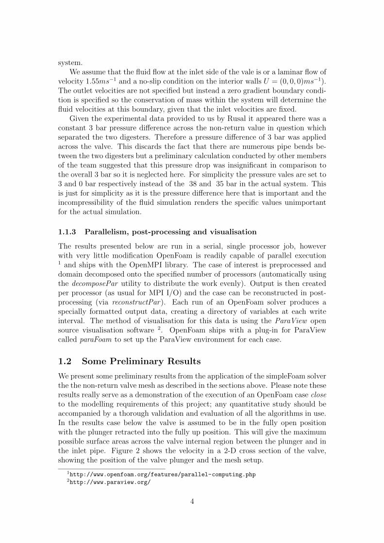
We present some preliminary results from the application of the simpleFoam solverthe the non-return valve mesh as described in the sections above. Please note theseresults really serve as a demonstration of the execution of an OpenFoam case closeto the modelling requirements of this project; any quantitative study should beaccompanied by a thorough validation and evaluation of all the algorithms in use.In the results case below the valve is assumed to be in the fully open positionwith the plunger retracted into the fully up position. This will give the maximumpossible surface areas across the valve internal region between the plunger and inthe inlet pipe. Figure 2 shows the velocity in a 2-D cross section of the valve,showing the position of the valve plunger and the mesh setup.

1http://www.openfoam.org/features/parallel-computing.php2http://www.paraview.org/

4

Figure 2: The velocity magnitude profile on a 2-D slice across the valve. NOTE: The inlet isat the bottom of the vertical pipe section with uniform inlet velocity 4ms−1.

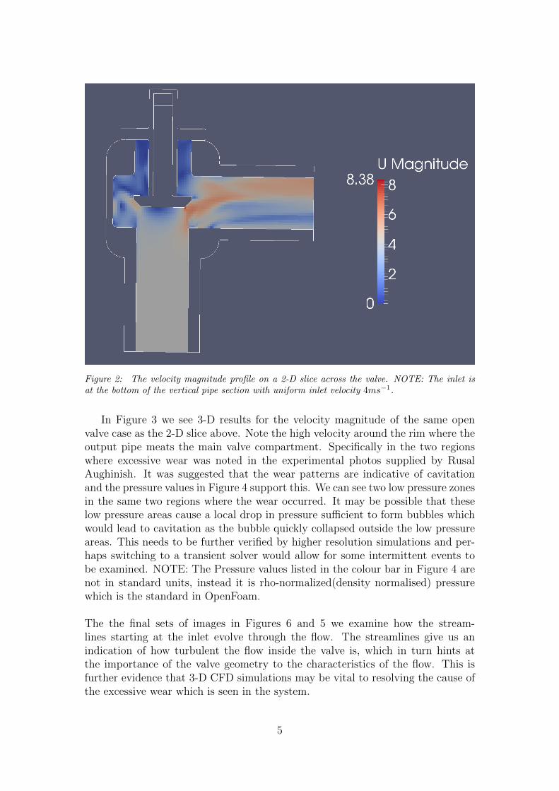
In Figure 3 we see 3-D results for the velocity magnitude of the same openvalve case as the 2-D slice above. Note the high velocity around the rim where theoutput pipe meats the main valve compartment. Specifically in the two regionswhere excessive wear was noted in the experimental photos supplied by RusalAughinish. It was suggested that the wear patterns are indicative of cavitationand the pressure values in Figure 4 support this. We can see two low pressure zonesin the same two regions where the wear occurred. It may be possible that theselow pressure areas cause a local drop in pressure sufficient to form bubbles whichwould lead to cavitation as the bubble quickly collapsed outside the low pressureareas. This needs to be further verified by higher resolution simulations and per-haps switching to a transient solver would allow for some intermittent events tobe examined. NOTE: The Pressure values listed in the colour bar in Figure 4 arenot in standard units, instead it is rho-normalized(density normalised) pressurewhich is the standard in OpenFoam.

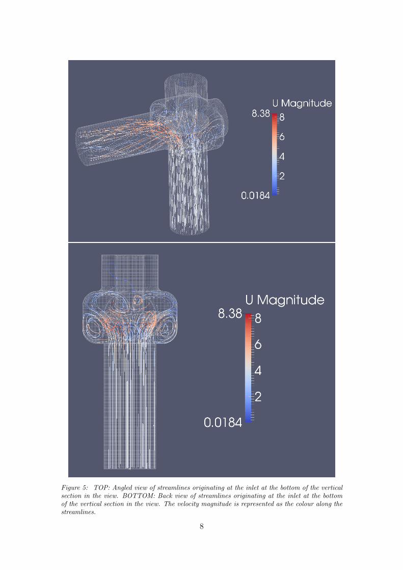
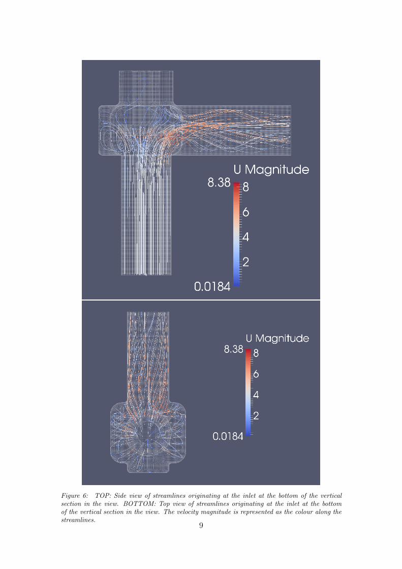
The the final sets of images in Figures 6 and 5 we examine how the stream-lines starting at the inlet evolve through the flow. The streamlines give us anindication of how turbulent the flow inside the valve is, which in turn hints atthe importance of the valve geometry to the characteristics of the flow. This isfurther evidence that 3-D CFD simulations may be vital to resolving the cause ofthe excessive wear which is seen in the system.

5

Figure 3: TOP: The velocity magnitude profile on the inner volume of the pipe/valve in the formof a wire-frame mesh. BOTTOM: The magnitude profile on the inner volume of the pipe/valvein the form of a wire-frame mesh. NOTE: The velocity magnitude units are ms−1.

6

Figure 4: TOP: The pressure profile on the inner volume of the pipe/valve in the form of awire-frame mesh. BOTTOM: The pressure profile on the inner volume of the pipe/valve in theform of a wire-frame mesh. NOTE: The Pressure values listed in the colour bar are not instandard units, instead it is rho-normalized(density normalised) pressure which is the standardin OpenFoam.

7

Figure 5: TOP: Angled view of streamlines originating at the inlet at the bottom of the verticalsection in the view. BOTTOM: Back view of streamlines originating at the inlet at the bottomof the vertical section in the view. The velocity magnitude is represented as the colour along thestreamlines.

8

Figure 6: TOP: Side view of streamlines originating at the inlet at the bottom of the verticalsection in the view. BOTTOM: Top view of streamlines originating at the inlet at the bottomof the vertical section in the view. The velocity magnitude is represented as the colour along thestreamlines.

9

1.3 Future developments

Opportunities for developing the method and validating the numerics are exten-sive. The first would be to utilise the parallel processing utilities of OpenFoamto allow the current simulations to be run in much higher resolution to furtherresolve the interesting areas in the system where the high velocity/local low pres-sures occur.As mentioned in a earlier section we discusse how the current results are for asteady state solution. However the OpenFoam software paskage has a numberof other solvers avaibale that can handle transient flows. These include pimple-Foam (large time-step transient solver for incompressible, flow using the PIMPLE(merged PISO-SIMPLE) algorithm) and pisoFoam (transient solver for incom-pressible flow) which both have the advantage of being able to observe intermit-tent events our steady state solver would not.However one would also expect such models to be extremely computationallydemanding and it is likely to require access to an HPC facility for serious compu-tations.

2 Conclusions

This part of this report has presented a potential approach for a direct numericalsimulation framework for the problem at hand. A first attempt at some simula-tion is presented using the OpenFOAM CFD software suite and a detailed CADdrawing of the valve to run a 3D incompressible fluid simulation to detect possibleproblem areas within the pipe. This is achieved numerically using a finite-volumediscretisation of the transport equations with a volume of fluid treatment of thephase fraction. The complexity of OpenFOAM is extensive and allows us to tacklea large number of the modelling requirements at hand. In particular we have shownthe ease of setting up the meshes to accommodate the complex internal geometryof the problem. The initial runs show the possible power of the method; alreadywe find some evidence that the geometry of the valve may be a significant con-tributing factor to apparent cavitation wear patterns in the Non-return valve.

Future work would involve greatly increasing the resolution and switching toa parallel mesh decomposition which would allow for more mesh cells to be in-cluded, improving the accuracy of the solution. It is our hope that the method andmodelling strategy presented allows the opportunity to investigate many of thesein a relatively short space of time as the OpenFoam framework has an extensiveparallel mesh decomposition toolbox as standard. In particular it is now a trivialexercise to vary inflow rates and pressure drops across the valves and examine thecorresponding characteristics of the resulting flow. In due course it is believedthe direct numerical simulation could help explain the problem proposed and alsoprevent future changes in valve and pipe geometry from causes such excessive wearproblems.

10

3 Installing and using OpenFOAM

In this appendix we provide some brief comments on installing and using Open-FOAM.

OpenFOAM can be built on a number of platforms but is easiest compiled ona Linux system. A large number of HPC systems will already have OpenFOAMinstalled (e.g. ICHEC in Ireland). Full documentation and instructions on theinstallation and use of the codes can be found online at 3. In short all of theresults we show here are created using standard solvers built at installation andfollowing a familiar pattern at runtime. The documentation shows how to set upa case 4 and several tutorials are provided to familiarise the user with the be-haviour of the code. We recommend running some simple relevant tutorial casesto get used to the format of OpenFOAM and ensure that the configuration youhave is working correctly. Accompanying file ”Rusal ESGI110.tar.gz” contains thecase files for setting up the mesh from the .STL CAD file and running the actualsimulation. Note for ease of use, and to ensure the correct sequence of set-upsteps, we have written some bash scripts to automate some of the set-up, calledAllrun.bash. These will hopefully be clear given the online OpenFOAM documen-tation.The OpenFOAM website also describes how to install ParaView and set upthe plugins to read OpenFOAM results.

Changing parameters of the problem will either be handled in the preprocessing(e.g. problem geometry in the .STL CAD Files) or in the individual case files (e.g.“0/U” for boundary conditions, “constant/Block meshDict” for the mesh density.)

References

[1] Peralta, C., Nugusse, H., Kokilavani, S.P., Schmidt, J., and Stoevesandt, B.Validation of the simplefoam (rans) solver for the atmospheric boundary layerin complex terrain. ITM Web of Conferences, 2:01002, 2014.

3http://www.openfoam.org/4http://www.openfoam.org/docs/user/cases.php

11